Asymptotic scaling and continuum limit of pure SU(3) lattice gauge theory

Abstract

Recently the Yang-Mills gradient flow of pure SU(3) lattice gauge theory has been calculated in the range from $\beta=6/g_{0}^{2}=6.3$ to 7.5 (Asakawa et al.), where $g_{0}^{2}$ is the bare coupling constant of the SU(3) Wilson action. Estimates of the deconfining phase transition are available from $\beta=5.7$ to 6.8 (Francis et al.). Here it is shown that the entire range from 5.7 to 7.5 is well described by a power series of the lattice spacing $a$ times the lambda lattice mass scale $\Lambda_{L}$, using asymptotic scaling in the 2-loop and 3-loop approximations for $a\Lambda_{L}$. In both cases identical ratios for gradient flows versus deconfinement observables are obtained. Differences in the normalization constants with respect to $\Lambda_{L}$ give a handle on their systematic errors.

I Introduction

We consider pure SU(N), $N=3$, lattice gauge theory (LGT) with the Wilson action (see, e.g., MM )

$$S\ =\ -\frac{\beta}{N}\,{\rm Re}\sum_{p}{\rm Tr}\,U_{p}\,,~{}~{}~{}\beta=\frac{2N}{g_{0}^{2}}\,,$$ (1)

where the sum is over all plaquettes of a 4D hypercubic lattice with periodic boundary conditions. $U_{p}$ is the SU(N) plaquette variable, $g^{2}_{0}$ the bare coupling constant and $\beta$ the usual convention, which emphasizes the interpretation as a 4D statistical mechanics, but gives up the $\beta=1/(kT)$ relation with the physical temperature. Namely, $T=1/(aN_{\tau})$ holds in LGT, where the integer $N_{\tau}$ is the extension of the lattice in Euclidean time and $a$ is the lattice spacing.

For every physical observable $m$ with the dimensions of a mass the relation

$$m\ =\ c_{m}\,\Lambda_{L}$$ (2)

holds in the continuum limit $a(\beta)\to 0$ for $\beta\to\infty$, where $\Lambda_{L}$ sets the mass scale of the lattice regularization and $c_{m}$ are calculable constants. Their actual computation faces difficulties, because one has to rely on simulations at finite lattice spacings $a(\beta)$, introducing corrections to the continuum relation. The subject of a good reference scale arises. This topic gained renewed interest after Lüscher L10 introduced the Yang-Mills gradient flow scale, $\sqrt{t_{0}}$, which comes by now in several variants. As anticipated by Sommer in his review of the subject So13 , gradient scales allow for an unprecedented precision, when compared with traditional scales like $r_{0}$ or $r_{c}$ NS02 defined by the force between static quarks at intermediate distance.

In recent work Asakawa et al. A15 pushed estimates for gradient scales in SU(3) gauge theory all the way up to $\beta=7.5$. The SU(3) deconfining phase transition defines another precise scale, second only to gradient scales. Francis et al. Fr15 managed to extend estimates of the SU(3) transition temperature $T_{t}$ from lattice sizes of previously $N_{\tau}\leq 12$ up to $N_{\tau}=22$, $\beta_{t}=6.7986\,(65)$.

Remarkably, neither Asakawa et al. nor Francis et al. fit the $\beta$ dependence of their estimates so that there is a $\beta\to\infty$ continuum limit as predicted by the universal part of asymptotic scaling. Instead, a parametrization for a limited $\beta$ range is used and the continuum limit of ratios is subsequently estimated by fits in variables like $(a/r_{0})^{2}$, $(a/\sqrt{t_{0}})^{2}$ and so on. This is in accord with a majority of publications on the subject, which all have given up on approaching the asymptotic scaling limit.

Reasons for this, and why the decision to give up on asymptotic scaling may have been premature, are outlined in section II. Inspired by an earlier approach of Allton A97 , we are led to write the corrections to the mass relation (2) as a simple Taylor series in the lattice spacing times the lambda lattice mass scale, $a\Lambda_{L}$. In section III this is seen to yield excellent results for fitting the data of Ref. A15 and Fr15 (see the abstract). Summary and conclusions follow in the final section IV.

II Asymptotic scaling and continuum limit

The realization that the continuum limit of LGT may not just in theory but in practice be reached by computer simulations started with a paper by Creutz C80 , where he observed for the SU(2) string tension $\kappa$ a cross-over from its strong coupling behavior $a^{2}\kappa=-\ln(\beta/4)$ to the 1-loop asymptotic scaling behavior $a^{2}\kappa=c_{\kappa}\,\exp(-6\pi^{2}\beta/11)$.

As the accuracy of Markov chain Monte Carlo calculations improved, it was soon realized that there were, in particular for SU(3) with the Wilson action, strong violations of the asymptotic scaling relation and this did not improve noticeably by moving from the 1-loop to the 2-loop relation

$$a\Lambda_{L}=f^{0}_{as}(g^{2}_{0})=\left(b_{0}\,g^{2}_{0}\right)^{-b_{1}/2b^{2}_{0}}\,\exp\left(-\frac{1}{2b_{0}g_{0}^{2}}\right)\,,$$ (3)

where $b_{0}=11\,N/(48\pi^{2})$ and $b_{1}=(34/3)\,N^{2}/(16\pi^{2})^{2}$ are, respectively, the universal 1-loop Gr73 ; Po73 and 2-loop Jo74 ; Ca74 coefficients of asymptotic freedom, called asymptotic scaling in our context. Universal means that all renormalization schemes lead to the same $b_{0}$ and $b_{1}$ coefficients.

Next, the hope appeared to be that the situation would improve by including further, non-universal, terms of the expansion of $a\Lambda_{L}$:

$$a\Lambda_{L} = f_{as}(g^{2}_{0})\ =\ f^{0}_{as}(g^{2}_{0})\,\left(1+\sum_{j=1}^{\infty}q_{j}\,g_{0}^{2j}\right)\,.$$ (4)

Computing up to 3-loops, Allés et al. AF97 calculated $q_{1}$ for SU(N) LGT,

$$q_{1}\ =\ 0.1896~{}~{}{\rm for\ SU(3)}\,.$$ (5)

But, the discrepancies between the asymptotic scaling equation and data for physical quantities did not improve.

Assuming that lattice artifacts are responsible for the disagreements, Allton A97 suggested to include such corrections while constraining them with results from perturbative expansions of the considered operators and actions. Doubting, due to uncertainties with the very definition of non-trivial continuum functional integrals, that perturbative information beyond Eq. (4) is reliable, a general Taylor series expansion in $a\Lambda_{L}$ is proposed here for corrections to Eq. (2),

$$m=c_{m}\,\Lambda_{L}\,\left(1+\sum_{i=1}^{\infty}\hat{a}_{i}\,(a\,\Lambda_{L})^{i}\right)\,,~{}a\Lambda_{L}=f_{as}(g_{0}^{2})\,,$$ (6)

where one has to determine the normalization constants $c_{m}$ and the expansion coefficients $\hat{a}_{i}$ by computer simulations. This has the potential to eliminate the essential singularity of the perturbative expansion at $g_{0}^{2}=0$. However, the full sum (4) for $f_{as}(g_{0}^{2})$ is not available. Instead, we have to work with approximations and define for $q=0,\,1,\dots$

$$a\Lambda^{q}_{L}=f^{q}_{as}(\beta)=f^{0}_{as}\left[g^{2}_{0}(\beta)\right]\,\left(1+\sum_{j=1}^{q}q_{j}\,\left[g_{0}^{2}(\beta)\right]^{j}\right),\$$ (7)

where we have presently the $q=0$ (2-loop) and $q=1$ (3-loop) asymptotic scaling functions $f^{q}_{as}$ at our disposal and a conjecture for $q_{2}$ if we believe in the Padé approximation made in Ref. G06 . It is instructive to consider the deconfining temperature $T_{t}$ as reference scale. Then $a(\beta_{t})=1/[N_{\tau}(\beta_{t})T_{t}]$ implies $\Lambda^{q}_{L}(\beta)=f^{q}_{as}(\beta)N_{\tau}(\beta)T_{t}$.

Now, if the analyticity (6) is true when using the full $f_{as}$, it cannot be true at finite $q$. This is, for instance, seen by assuming that the expansion (6) is correct for $f^{1}_{as}$ and comparing it with the same expansion using $f^{0}_{as}$. The difference lies in terms of the form

$$\left(f^{0}_{as}\right)^{i}\left[\left(1+q_{1}\,g_{0}^{2}\right)^{i}-1\right]\,.$$ (8)

Expressing $g_{0}^{2}$ by $f^{0}_{as}$ gives rise to powers of logarithms like $1/\ln(f^{0}_{as})$, $\ln|\ln(f^{0}_{as})|$ and so on, which are singular for $f^{0}_{as}\to\infty$. Nevertheless, we continue to use (6) with $f_{as}$ replaced by $f^{q}_{as}$ and come back to these issues after presenting the fits.

In the following we consider observables with the dimension of a length, $L\sim 1/m$ and rewrite (6) as

$$\frac{L_{k}}{a} = c_{k}\,\left[a\,\Lambda_{L}\,\left(1+\sum_{i=1}^{\infty}\hat{a}_{i}\,(a\,\Lambda_{L})^{i}\right)\right]^{-1}\,$$ (9)

$$= \frac{c_{k}}{f_{as}(g_{0}^{2})}\,\left(1+\sum_{i=1}^{\infty}a_{i}\,[f_{as}(g_{0}^{2})]^{i}\right)\,,$$ (10)

where $a_{i}$ are the parameters with which we deal in our fits. There is no strong reason for using the expansion (10) instead of (9). It just developed this way out of Ref. A97 . To determine the expansion parameters $a_{i}$ by numerical calculations one has to truncate the sum at rather small values of $i$. For sufficiently large $\beta$ this should work well because $(a\Lambda^{q}_{L})$ falls for all $q$ exponentially off with $\beta\to\infty$. We define the truncated functions,

$$l^{p,q}_{\lambda}(\beta) = \frac{1}{f^{q}_{as}(\beta)}+\sum_{i=1}^{p}a_{i}^{p,q}\,\left[f^{q}_{as}(\beta)\right]^{i-1}\,,$$ (11)

with $f^{q}_{as}$ given by (7) and fit data according to

$$\frac{L_{k}}{a\,c_{k}^{p,q}} = l^{p,q}_{\lambda}(\beta)\,,$$ (12)

where the 2-loop ($q=0$) and 3-loop ($q=1$) asymptotic scaling functions, $l^{0,0}_{\lambda}$ and $l^{0,1}_{\lambda}$, are explicitly known (7). The labels $p,q$ on the normalization constants $c_{k}$ and parameters $a_{i}$ indicate that their values depend on the choice of $p,q$. For simplicity the labels will be dropped when the association is obvious.

For $q=0$ as well as for $q=1$ it turns out that excellent fits are obtained using $p=3$ parameters $a_{i}$ besides the $c_{k}$ normalization constants. In the following we present $l^{3,q}_{\lambda}$, $q=0,1$, expansions for the Yang-Mills gradient flow data A15 and for the deconfining transition estimates Fr15 .

III Analysis of the numerical data

Table 1: Error bars in percent of the signal, $100\,\triangle L_{k}/L_{k}$.

	$L_{1}$	$L_{2}$	$L_{3}$	$L_{4}$	$L_{5}$	$L_{6}$		$L_{7}$
$\beta$	$\sqrt{t_{0.2}}$	$\sqrt{t_{0.3}}$	$\sqrt{t_{0.4}}$	$w_{0.2}$	$w_{0.3}$	$w_{0.4}$	$\beta_{t}$	$N_{\tau}$
6.3	0.09	0.11	0.12	0.16	0.17	0.22	5.69275	0.07
6.4	0.07	0.09	0.08	0.11	0.12	0.14	5.89425	0.05
6.5	0.13	0.16	0.19	0.22	0.21	0.24	6.06239	0.06
6.6	0.12	0.14	0.16	0.19	0.21	0.23	6.20873	0.07
6.7	0.26	0.33	0.35	0.40	0.46	0.49	6.33514	0.06
6.8	0.18	0.22	0.25	0.27	0.30	0.32	6.4473	0.25
6.9	0.46	0.57	0.65	0.73	0.81	0.87	6.5457	0.54
7.0	0.14	0.17	0.19	0.21	0.25	0.26	6.6331	0.26
7.2	0.43	0.52	0.59	0.65	0.71	0.75	6.7132	0.34
7.4	0.30	0.34		0.41	0.50		6.7986	0.84
7.5	0.37			0.62
$n_{k}$	11	10	9	11	10	9		10

For the gradient length scale a dimensionless variable $t^{2}\langle E(t)\rangle$ is measured as a function of $t$. Then $t_{X}$ at which the observable takes a specific value $X$ is used as reference scale. An operator whose $t$ dependence has been extensively studied is $E(t)=F^{a}_{\mu\nu}F^{a}_{\mu\nu}/4$, where $F_{\mu\nu}=\partial_{\mu}A_{\nu}-\partial_{\nu}A_{\mu}+[A_{\mu},A_{\nu}]$ is the field strength. In Ref. A15 solutions to the equations

$$\left.t^{2}\langle E(t)\rangle\right|_{t=t_{X}}=X~{}~{}{\rm and}~{}~{}\left.t^{2}\frac{d\,}{dt}t^{2}\langle E(t)\rangle\right|_{t=w^{2}_{X}}=X$$ (13)

have been calculated for $X=0.2,\,0.3$ and $0.4$. The associated length scales are $\sqrt{t_{0.2}}$, $\sqrt{t_{0.3}}$, $\sqrt{t_{0.4}}$ and, introduced in Bo12 , $w_{0.2}$, $w_{0.3}$, $w_{0.4}$. For adaption to Eq. (12) they are renamed into $L_{1},\dots,L_{6}$ according to the first two rows of Table 1. Their estimates are given in Table 1 of A15 and are not reproduced here. Instead, we give in our Table 1 error bars in percent of the signal, $100\,\triangle L_{k}/L_{k}$, for the data tagged by a $*$ in their paper, i.e., used in their analysis.

Estimates of the SU(3) deconfining phase transition couplings $\beta_{t}$ are given in Table I of Ref. Fr15 . Whenever (for smaller lattices) a comparison is possible their estimates are consistent with previous work Bo96 ; BW13 .The lengths associated with the deconfining phase transition temperatures $T_{t}$ are $1/(aT_{t})=N_{\tau}$. However, the statistical errors are in $\beta_{t}$ with $N_{\tau}$ fixed. To allow for direct comparison with the other quantities, we attach to $N_{\tau}$ error bars relying on the later estimated $l^{3,1}_{\lambda}(\beta)$ scaling behavior from all data sets

$$\triangle N_{\tau}\ =\ N_{\tau}\,\left[l^{3,1}_{\lambda}(\beta_{t}+\triangle\beta_{t})-l^{3,1}_{\lambda}(\beta_{t})\right]/\ l^{3,1}_{\lambda}(\beta_{t})\,.$$ (14)

Starting with a guess and iterating the fit, one finds rapid convergence to the relative errors compiled in the $L_{7}$ column of Table 1. They are less than 0.25 for $\beta_{t}\leq 6.33514$ ($N_{\tau}\leq 12$) and $\geq 0.25$ for $\beta_{t}\geq 6.4473$ ($N_{\tau}\!=\!14,\dots,22$), implying that the fit parameters will be dominated by the smaller $\beta_{t}$ values. This is not good as the truncated parts of our expansion (11) become more important at smaller $\beta$. Therefore, we adjust the $L_{7}$ error bars for the lower $N_{\tau}$ to $100\,\triangle L_{7}/L_{7}=0.2$, which is still smaller than the best of the relative errors at the higher $N_{\tau}$ values.

For the gradient flow data the bias from smaller relative errors is less severe and with $\beta=6.3$ the smallest $\beta$ is not so small. No adjustments are made in that case.

Table 2: $\chi^{2}_{dof}$ for our fits to each of the length scales.

$q$	$L_{1}$	$L_{2}$	$L_{3}$	$L_{4}$	$L_{5}$	$L_{6}$	$L_{7}$
0	0.46	0.34	0.23	0.40	0.47	0.39	0.76
1	0.42	0.32	0.24	0.38	0.46	0.39	0.74

The $\chi^{2}_{dof}$ values of our fits (12) to the seven length scales are compiled in Table 2 ($n_{dof}=n_{k}-4$ with $n_{k}$ given in the last row of Table 1). All fits are in very good agreement with the data. Actually, the fits of the gradient flows are in too good agreement. This could be an accident, measurements of $L_{1}$ to $L_{6}$ were performed on the same configurations so that they are all correlated, or their error bars are systematically somewhat too large.

For a visual presentation we have combined the entire $n=n_{1}+\dots+n_{7}=70$ data into two $l^{3,q}_{\lambda}(\beta)$, $q=0,\,1$, fits for $L_{k}/(ac_{k})$, which works astonishingly well. This is done with an extension of the method of BB15 . The constants $c_{k}$ are defined as functions $c_{k}(a_{1},a_{2},a_{3};data)$, which give the exact minimum of the fit for the particular constants $a_{i}$, effectively reducing the fitting procedure to three parameters, though the $c_{k}$ are still counting against the degrees of freedom. The number of $a_{i}$ parameters is reduced by $6\times 3$ to 3 from the $7\times 3$ $a_{i}$ parameters used altogether for the fits of Table 2.

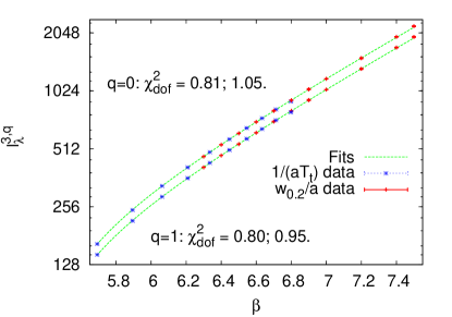
Figure 1: Data for $L_{7}/(c_{7}a)$ and $L_{4}/(c_{4}a)$ versus the $l^{3,q}_{\lambda}$ fits (12) using the 2-loop $f^{0}_{as}$ ($q=0$) and the 3-loop $f^{1}_{as}$ ($q=1$) asymptotic scaling functions.

In Fig. 1 the two fits are shown jointly with the data points ($i=1,\dots,n_{k}$)

$$\frac{L_{k}}{a\,c_{k}}(i)\pm\frac{\triangle L_{k}}{a\,c_{k}}(i)~{}~{}{\rm for}~{}~{}k=4,\,7\,.$$ (15)

Both fits cover with splendid $\chi^{2}_{dof}$ values the impressive range $5.69275\leq\beta\leq 7.5$. One value of $k$ is picked for the gradient flow, because on the scale of the figure the data for the other $L_{k}/(ac_{k})$ lie right on top of them. For each $q$ the first $\chi^{2}_{dof}$ value is for a fit that excludes the $1/(aT_{t})$ deconfinement data and the second $\chi^{2}_{dof}$ value for the shown fit, which includes them. However, the increase from the $\chi^{2}_{dof}$ values of Table 2 should be noted. This and the fact that the data of $L_{1}$ to $L_{6}$ are all correlated, as well as our “improvement” of the deconfinement data, may well obscure differences of the $a_{i}$ parameters for distinct observables. In fact, it is obvious from Fig. 4 (right) of Ref. A15 that correlations greatly reduce the error bars of ratios and that $\sqrt{t_{0.3}}/w_{0.4}$ is not entirely flat as in our fits. To take these correlations into account one would best jackknife our fits, which requires the original time series. In the present context of simply demonstrating the almost identical scaling of all data graphically this would just be a distraction. Generally, one expects the $a_{1}$ parameters to agree for all $L_{k}$, so that corrections to ratios are of order $(a\Lambda^{q}_{L})^{2}$. There is no reason for $a_{2}$ or $a_{3}$ to agree for all $L_{k}$. Only, it can be enforced within the accuracy of the present data. When these fits are applied to a single data set there is then a small bias due to the input of the other data sets.

To make Fig. 1 reproducible, the fit parameters are given with high precision in Table 3. More decent values are obtained when one redefines the expansion parameters $a\Lambda^{q}_{L}$ by multiplicative constants, e.g., so that they become 1 at $\beta=6$, $x^{q}(\beta)=f^{q}_{as}(\beta)/f^{q}_{as}(6)$. The second row of Table 3 gives the fits parameters for this case with their error bars in the third row. The range covered by the $x^{q}(\beta)$ goes from $x^{q}(5.7)\approx 1.4$ down to $x^{q}(7.5)\approx 0.18$, so that $x^{q}(7.5)^{2}\approx 0.032$ and $x^{q}(7.5)^{3}\approx 0.0058$ become really small.

Table 3: Fit parameters used for Fig. 1.

$a^{3,0}_{1}$	$a^{3,0}_{2}$	$a^{3,0}_{3}$	$a^{3,1}_{1}$	$a^{3,1}_{2}$	$a^{3,1}_{3}$
$-$155.559	24615.3	$-$5834850	$-$104.735	9926.28	$-$2673493
$-$0.365	0.135	$-$0.754	$-$0.292	0.773	$-$0.581
(13)	(20)	(82)	(13)	(42)	(82)

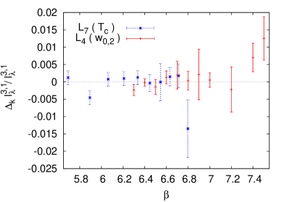
Figure 2: Relative deviations (16) of the $L_{7}$ and $L_{4}$ data points from the $l^{3,1}_{\lambda}$ fit.

Fig. 2 provides a visual impression for the quality of the fits, by plotting the deviations of the $k=4$ and 7 data points from the $q=1$ fit of Fig. 1 in the form

$$\frac{\triangle_{k}l^{3,1}_{\lambda}(i)}{l^{3,1}_{\lambda}(\beta_{i})}~{}~{}{\rm with}~{}~{}\triangle_{k}l^{p,q}_{\lambda}(i)=\frac{L_{k}}{a\,c_{k}}(i)-l^{p,q}_{\lambda}(\beta_{i})$$ (16)

together with error bars $\triangle L_{k}/(ac_{k}l^{3,1}_{\lambda})$.

Table 4: Normalization constants $c_{k}\times 100$.

$q$	0	1	0	1
$c_{1}$	0.4918 (37)	0.5569 (41)	0.492 (06)	0.557 (07)
$c_{2}$	0.6198 (46)	0.7018 (52)	0.619 (11)	0.701 (12)
$c_{3}$	0.7152 (53)	0.8099 (59)	0.695 (25)	0.789 (28)
$c_{4}$	0.5392 (40)	0.6106 (45)	0.548 (10)	0.620 (11)
$c_{5}$	0.6304 (47)	0.7139 (52)	0.638 (16)	0.722 (17)
$c_{6}$	0.7028 (53)	0.7958 (59)	0.679 (34)	0.771 (38)
$c_{7}$	2.4404 (71)	2.7754 (79)	2.357 (46)	2.693 (51)

Perhaps surprisingly, instead of one satisfactory description of the data we got two (seven more pairs for the fits with their $\chi^{2}_{dof}$ values listed in Table 2). The quality of the fits does not care about the log corrections discussed after Eq. (8). Instead, the parameters adjust and the normalization constants $c_{1}$ to $c_{7}$ get shifted as shown in Table 4. Here the numbers in column 2 and 3 correspond to the joint fits of the six gradient flow operators, with exception of the last row, which corresponds to the fits displayed in Fig. 1 for which all seven operators are combined. Columns 4 and 5 give the results obtained from individual fits to which one should fall back when it comes to conservative estimates. Normalization constants of corresponding $q=0,1$ fits differ by about 12%, while their statistical errors are much smaller.

Table 5: Ratios of normalization constants.

$q$	0	1	0	1
$c^{1}_{7}$	0.19728 (22)	0.19724 (22)	0.209 (05)	0.207 (05)
$c^{2}_{7}$	0.24861 (28)	0.24856 (28)	0.263 (07)	0.260 (07)
$c^{3}_{7}$	0.28689 (33)	0.28683 (33)	0.295 (12)	0.293 (12)
$c^{4}_{7}$	0.21630 (26)	0.21625 (26)	0.233 (07)	0.230 (06)
$c^{5}_{7}$	0.25288 (32)	0.25283 (32)	0.271 (09)	0.268 (09)
$c^{6}_{7}$	0.28188 (37)	0.28182 (37)	0.288 (16)	0.286 (15)

For ratios, $c^{k}_{l}=c_{k}/c_{l}$, of the normalization constants these differences become tiny and are swallowed by the statistical error bars as is seen in Table 5 for $c^{k}_{7}$ (columns are arranged as in Table 4). The deconfining transition is used as reference scale, because $L_{7}$ is statistically independent from $L_{1}$ to $L_{6}$. The estimates of the last row can be compared with Asakawa et al. A15 . Using $q=1$, our values $c^{6}_{7}=w_{0.4}T_{t}=0.28182\,(37)$ and $0.286\,(15)$ are both well consistent with $0.285\,(5)$ as given in their Table 3. Our value from column 3 is inconsistent with the precise estimate given in their Eq. (3.2), $0.2826\,(3)$. The discrepancy may be well explained by the small bias of our result and/or the fact that Asakawa et al. rely entirely on $N_{\tau}=12$, whereas here a continuum fit is used that gives weight to all lattices, including $N_{\tau}=14$ to 22.

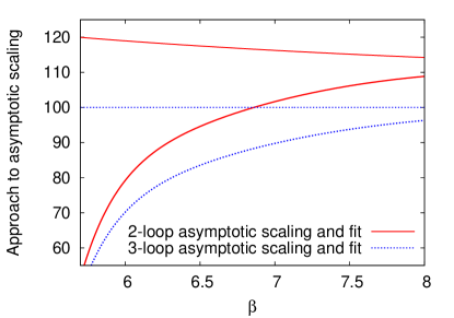
Figure 3: Approach of the $l^{3,q}_{\lambda}$ fits to the asymptotic 2-loop and 3-loop scaling functions $l^{0,q}_{\lambda}$ ($q=0,1$) times $100/l^{0,1}_{\lambda}$.

The $\chi^{2}_{dof}$ of the fits (12) are not sensitive to including or not including the $q_{1}g_{0}^{2}$ term into the scaling function (7), while there is a remarkable shift in the normalization constants. It is then tempting, but entirely wrong, to argue that the $g_{0}^{2}$ dependence is so weak that it does not matter and one could replace $q_{1}g_{0}^{2}$ by a constant, say $q_{1}g_{0}^{2}\to q_{1}^{c}=0.9\,q_{1}$ for our $\beta$ range. It is easy to see that with this, or any other $q_{1}^{c}$, the normalization constants of the $q=0$ fits will not change at all. So, the shift in the normalization constants comes entirely from the $g_{0}^{2}$ dependence of the $q_{1}$ term. These contributions re-sum in a way that they become for large $\beta$ responsible for the difference between $l^{0,1}_{\lambda}$ and $l^{0,0}_{\lambda}$.

We use our fits of all $n=70$ data to illuminate the situation by Fig. 3, where for $q=0,1$ the inverse asymptotic scaling functions $l^{0,q}_{\lambda}$ and their $l^{3,q}_{\lambda}$ fits are plotted times $100/\,l^{0,1}_{\lambda}$, i.e., as fractions of the inverse 3-loop asymptotic scaling function $l^{0,1}_{\lambda}$. We see that the gap between the $l^{0,0}_{\lambda}$ and $l^{0,1}_{\lambda}$ asymptotic scaling functions narrows slowly and the fits $l^{3,0}_{\lambda}$ and $l^{3,1}_{\lambda}$ approach rapidly (exponentially fast for increasing $\beta$) their respective asymptotic behaviors, where the $l^{3,1}_{\lambda}$ fit stays closer to its asymptotic form than the $l^{3,0}_{\lambda}$ fit: $l^{0,1}_{\lambda}/l^{3,1}_{\lambda}\approx 0.8\,l^{0,0}_{\lambda}/l^{3,0}_{\lambda}$ over the entire $\beta$ range of the figure..

How does it come that the data cannot figure out whether the $q=0$ or $q=1$ fit is better? The answer lies in their ratios: If the ratio of the two fits is a constant, the difference between them will be entirely absorbed by the normalization. Defining the change in the ratios with respect to $\beta=6$ as reference point by

$$d^{p}(\beta)\ =\ 100\,\left(1-\frac{l^{p,0}_{\lambda}(\beta)/l^{p,1}_{\lambda}(\beta)}{l^{p,0}_{\lambda}(6)/l^{p,1}_{\lambda}(6)}\right)\,,$$ (17)

we find for the asymptotic scaling ($p=0$) functions a change by 3.2% at $\beta=7.5$. With 0.16% it is twenty times smaller for the fits ($p=3$).

What is then the effect of including more and more $q_{j}$ terms in the expansion (4) of $f_{as}$? We may expect convergence of the resulting normalization constants $c_{k}$ towards their correct value. But how fast? Repeating the fits of all data with fake $f^{2}_{as}$ functions (7) defined by $q_{2}=\pm 0.19$, so that $q_{2}$ has a similar absolute value as $q_{1}$, there is again no sensitivity of the $\chi^{2}_{dof}$ of the fits for the additional term and corrections to the $c_{k}$ normalization constants stay less than $\pm 10$%. On this basis we end up with the result that our most reliable estimates of the $c_{k}$ are those of column five of Table 4 with a mainly systematic uncertainty of $\pm 10$%. From $c_{7}$ we get

$$\Lambda^{1}_{L}/T_{t}\ =\ c_{7}\pm 10\%\ =\ 0.0269\ (27)\,$$ (18)

in good agreement with Francis et al. Fr15 , who give $T_{t}/\Lambda_{\overline{M}S}=1.24\,(10)$. Using standard relations between lambda scales MM this becomes $\Lambda_{L}/T_{t}=0.0280\,(25)$. Similarly, our estimate for $w_{0.4}\Lambda_{L}$,

$$L_{6}\Lambda^{1}_{L}\ =\ c_{6}\pm 10\%\ =\ 0.0077\ (9)\,,$$ (19)

is in agreement with the one of Table 3 of Asakawa et al. A15 and the more accurate value of their Eq. (3.3), which translate, respectively, into $w_{0.4}\Lambda_{L}=0.00809\,(35)$ and $w_{0.4}\Lambda_{L}=0.00829\,(5)$.

When we believe in the Padé approximation of G06 , we find $q_{2}=-0.02467$, which is in magnitude almost ten times smaller than the range we allowed for our estimate of the systematic error. Using then fits with $f^{2}_{as}(\beta)$ as reference, Eq. (18) and (19) improve to

$$\Lambda^{2}_{L}/T_{t}=0.0266\ (9)~{}~{}{\rm and}~{}~{}L_{6}\Lambda^{2}_{L}=0.00762\ (45)\,,$$ (20)

where contributions of the statistical errors exceed now the systematic errors. So, it is difficult to understand why the error in Eq. 3.3 of Asakawa et al. is much smaller. Anyway, a small $q_{2}$ suggests rapid convergence of the systematic errors of the normalization constants under increasing $q$ for the used $f^{q}_{as}$ functions.

IV Summary and conclusions

It appears that Eq. (6) is a natural parametrization of lattice spacing corrections to the continuum limit of SU(3) LGT. Incorporation of asymptotic scaling is still a viable alternative to other fitting methods for the approach to the continuum limit, which are utilized in A15 ; Fr15 and elsewhere. In a next step, our fitting procedure should be tested for other asymptotically free theories, in particular full QCD.

- (1) I. Montvay and G. Münster, Quantum Fields on a Lattice, Cambridge University Press, 1994.
- (2) M. Lüscher, JHEP 08, 071 (2010); 03, 092(E) 2014.
- (3) R. Sommer, POS (Lattice 2013) 015.
- (4) S. Necco and R. Sommer, Nucl. Phys. B 622 (2002) 328.
- (5) M. Asakawa, T. Hatsuda, T. Iritani, E. Itou, M. Kitazawa, and H. Suzuki, arXiv:1503.06516v2.
- (6) A. Francis, O. Kaczmarek, M. Laine, T. Neuhaus, and H. Ohno, Phys. Rev. D 91, 096002 (2015).
- (7) C.R. Allton, Nucl. Phys. B (Proc. Suppl.) 53, 867 (1997).
- (8) M. Creutz, Phys. Rev. D 21, 2308 (1980).
- (9) D.J. Gross and F. Wilczek, Phys. Rev. Lett. 30, 1343 (1973).
- (10) H.D. Politzer, Phys. Rev. Lett. 30, 1346 (1973).
- (11) D.R.T. Jones, Nucl. Phys. B 75, 531 (1974).
- (12) W. Caswell, Phys. Rev. Lett. 33, 244 (1974).
- (13) B. Allés, A. Feo and H. Panagopoulos, Nucl. Phys. B 491, 498 (1997).
- (14) M. Göckeler, R. Horsley, A.C. Irving, D. Pleiter, P.E.L. Rakow, G. Schierholz, and H. Stüben, Phys. Rev. D 73, 014513 (2006).
- (15) S. Borsányi, S. Dürr, Z. Fodor, C. Hoebling, S.D. Katz, S. Krieg, T. Kurth, L. Lellouch, T. Lippert, C. McNeile, and K.K. Szabó, JHEP 09, 010 (2012).
- (16) G. Boyd, J. Engels, F. Karsch, E. Laermann, C. Legeland, M. Lütgemeyer and B. Peterson, Nucl. Phys. B 469, 419 (1996).
- (17) B.A. Berg and H. Wu, Phys. Rev. D 88, 074507 (2013).
- (18) B.A. Berg, arXiv:1505.07564, submitted to CPC.