Effects of strong magnetic fields and rotation on white dwarf structure

Abstract

In this work we compute models for relativistic white dwarfs in the presence of strong magnetic fields. These models possibly contribute to super-luminous SNIa. With an assumed axi-symmetric and poloidal magnetic field, we study the possibility of existence of super-Chandrasekhar magnetized white dwarfs by solving numerically the Einstein-Maxwell equations, by means of a pseudo-spectral method. We obtain a self-consistent rotating and non-rotating magnetized white dwarf models. According to our results, a maximum mass for a static magnetized white dwarf is 2.13 $\rm{M_{\odot}}$ in the Newtonian case and 2.09 $\rm{M_{\odot}}$ while taking into account general relativistic effects. Furthermore, we present results for rotating magnetized white dwarfs. The maximum magnetic field strength reached at the center of white dwarfs is of the order of $10^{15}\,$G in the static case, whereas for magnetized white dwarfs, rotating with the Keplerian angular velocity, is of the order of $10^{14}\,$G.

I Introduction

White dwarfs (WDs) are stellar remnants of stars with masses of up to several solar masses. With a mass comparable to that of the Sun $\sim 2\times 10^{33}\,\rm{g}$, which is distributed in a volume comparable to that of the Earth, the central mass density in these objects can reach values of about $10^{11}\,\rm{g/cm^{3}}$. Together with neutron stars and black holes, they are the endpoints of stellar evolutions and play a key role in astrophysics Shapiro and Teukolsky (2008); Glendenning (2012).

The existence of white dwarfs was one of the major puzzles in astrophysics until Fowler Fowler (1926), based on the quantum-statistical theory developed by Fermi and Dirac Dirac (1926); Fermi (1926), shows that white dwarfs are supported by the pressure of a degenerate electron gas. In addition, Chandrasekhar in Ref. Chandrasekhar (1931) included effects of special relativity in the degenerate electron gas theory and, as a result, found that there is a limit in the stellar mass, above which degenerate white dwarfs are unstable. This critical mass is the so-called Chandrasekhar limit and is about 1.4 $\rm{M_{\odot}}$.

White dwarfs are mostly composed of electron-degenerate matter. The mass of the star is essentially due to the nuclei, whereas the main contribution to the pressure comes from the electrons. For typical WDs, thermonuclear reactions terminate at lighter nuclei, as Carbon, helium, or oxygen Chandrasekhar (1939); Glendenning (2012).

Some white dwarfs are also associated with strong magnetic fields. From observations, the surface magnetic field of these stars can reach values from $10^{6}\,$ G to $10^{9}\,$ G Terada et al. (2008); Reimers et al. (1996); Schmidt and Smith (1995); Kemp et al. (1970); Putney (1995). However, the internal magnetic field in magnetic stars is very poorly constrained by the observations and can be much stronger than in the surface. For example, white dwarfs can have internal magnetic fields as large as $10^{12-16}\,$ G according to Refs. Angel (1978); Shapiro and Teukolsky (2008); Bera and Bhattacharya (2014). Moreover, self-consistently highly magnetized neutron stars calculations have shown that neutron stars can possess central magnetic fields as large as $10^{18}\,$ G Bocquet et al. (1995); Chatterjee et al. (2015); Cardall et al. (2001); Franzon et al. (2015). Therefore, understanding and estimating magnetic fields inside compact objects occupy a key position in astrophysics.

Motivated by observations of a thermonuclear supernova that appears to be more luminous than expected (e.g. SN 2003fg, SN 2006gz, SN 2007if, SN 2009dc), it has been argued Scalzo et al. (2010); Howell et al. (2006); Hicken et al. (2007); Yamanaka et al. (2009); Taubenberger et al. (2011) that the progenitor of such super-novae should be a white dwarf with mass above the well-known Chandrasekhar limit, in other words, a super-Chandrasekhar white dwarf.

Progenitors with masses $\rm{M>2.0\,\,\rm{M_{\odot}}}$ were considered in the literature as a result of mergers of two massive white dwarfs, or due to fast rotation Moll et al. (2014). In addition, super-Chandrasekhar white dwarfs were investigated in a strong magnetic field regime as in Refs. Das and Mukhopadhyay (2012, 2013, 2014). In the Newtonian framework, models for white dwarfs endowed with a magnetic field and/or rotating were investigated in a series of papers Adam (1986); Ostriker and Bodenheimer (1968); Ostriker and Hartwick (1968); Ostriker and Tassoul (1969). Recently, a study of differentially rotating and magnetized white dwarfs were performed within the ideal magnetohydrodynamic (GRMHD) regime Subramanian and Mukhopadhyay (2015) and they have found that differential rotation can increase the mass of magnetized white dwarfs up to 3.1 $\rm{M_{\odot}}$.

In Ref. Das and Mukhopadhyay (2013), it was obtained ultramagnetized white dwarfs with a maximum mass of 2.58 $\rm{M_{\odot}}$. The authors also found a magnetic field strength up to $10^{18}\,$G at the center of the star. Nonetheless, such approach violates not only macro physics aspects, as for example, the breaking of spherical symmetry due to the magnetic field, but also micro physics considerations, which are relevant for a self-consistent calculations of the structure of these objects Coelho et al. (2014); Chamel et al. (2013); Nityananda and Konar (2015). Besides, a self-consistently newtonian structure calculation of strongly magnetized white dwarfs shown that these stars exceed the traditional Chandrasekhar mass limit significantly $(\rm{M\sim 1.9\,M_{\odot}})$ for a maximum field strength of the order of $\rm{10^{14}\,}$G Bera and Bhattacharya (2014).

In this work, we model static and rotating magnetized white dwarfs in a self-consistent way by solving Einstein-Maxwell equations in the same way as done originally for neutron stars in Refs. Bonazzola et al. (1993); Bocquet et al. (1995). We follow also our recent work on highly magnetized hybrid stars Franzon et al. (2015), where both general relativistic effects and the anisotropy of the energy momentum tensor caused by the magnetic field were taken into consideration to calculate the star structure. The presence of such a strong magnetic field can locally affect the microphysics of the equation of state (EoS), as for example, due to Landau quantization. As shown in Ref. Bera and Bhattacharya (2014), the Landau quantization does not affect the global properties of white dwarfs. However, the authors solve the structure equation in a Newtonian form and without the magnetization term for the matter. Moreover, as we will see, effects of general relativity can play an important role by determining the maximum mass of such highly magnetized white dwarfs.

Globally, the magnetic field can affect the structure of WDs since it contributes to the Lorenz force, which acts against gravity. In addition, it contributes also to the structure of the spacetime, since the magnetic field is now a source for the gravitational field through the Maxwell energy-momentum tensor. As we are interested in global effects that magnetic fields and the rotation can induce in WDs, we simplify the discussion assuming white dwarfs composed predominately by ${}^{12}C$ ($A/Z=2$) in a electron background .

II Basic equations and formalism

In this work, we consider rotating and non-rotating magnetized white dwarfs. The formalism used here was first applied to stationary neutron stars Bonazzola et al. (1993); Bocquet et al. (1995); Chatterjee et al. (2015) and more recently in Ref. Franzon et al. (2015). Details of the gravitational equations, numerical procedure and other properties of the equations can be found in the references cited above and in Ref. Gourgoulhon (2012). For the sake of completeness and for a better understanding of the reader, we show here some of the electromagnetic equations that, together with the gravitational equations, are solved numerically. The energy-momentum tensor of the system reads:

$$T_{\alpha\beta}=(e+p)u_{\alpha}u_{\beta}+pg_{\alpha\beta}+\frac{1}{\mu_{0}}\left(F_{\alpha\mu}F^{\mu}_{\beta}-\frac{1}{4}F_{\mu\nu}F^{\mu\nu}\mathrm{g}_{\alpha\beta}\right),$$ (1)

where $F_{\alpha\mu}$ denotes the antisymmetric Faraday tensor, $e$ the energy density and $p$ the pressure as measured by an observer ($\mathcal{O}_{1}$) co-moving with the fluid and whose four-velocity is $u_{\alpha}$. The $g_{\alpha\beta}$ is the metric tensor. The first term in Eq. (1) is the isotropic matter contribution to the energy momentum-tensor, while the second term is the anisotropic electromagnetic field contribution.

The electromagnetic contribution (EM) to the energy-momentum tensor is obtained within the so-called 3+1 decomposition Gourgoulhon (2012); Bonazzola et al. (1993). The energy density becomes:

$$E^{(EM)}=\frac{1}{2\mu_{0}}(E^{i}E_{i}+B^{i}B_{i}),$$ (2)

and the momentum-density flux can be written as:

$$J^{(EM)}_{\phi}=\frac{1}{\mu_{0}}A^{2}(B^{r}E^{\theta}-E^{r}B^{\theta}).$$ (3)

The stress 3-tensor components are given by:

$$S^{(EM)r}_{\;\;\;r}=\frac{1}{2\mu_{0}}(E^{\theta}E_{\theta}-E^{r}E_{r}+B^{\theta}B_{\theta}-B^{r}B_{r}),$$ (4)

$$S^{(EM)\theta}_{\;\;\;\theta}=\frac{1}{2\mu_{0}}(E^{r}E_{r}-E^{\theta}E_{\theta}+B^{r}B_{r}-B^{\theta}B_{\theta}),$$ (5)

$$S^{(EM)\phi}_{\;\;\;\phi}=\frac{1}{2\mu_{0}}(E^{i}E_{i}+B^{i}B_{i}),$$ (6)

being the electric field components, as measured by the Eulerian observer $\mathcal{O}_{0}$, written as Lichnerowicz et al. (1967):

$$E_{\alpha}=\left(0,\frac{1}{N}\left[\frac{\partial A_{t}}{\partial r}+N^{\phi}\frac{\partial A_{\phi}}{\partial r}\right],\frac{1}{N}\left[\frac{\partial A_{t}}{\partial\theta}+N^{\phi}\frac{\partial A_{\phi}}{\partial\theta}\right],0\right),$$ (7)

and the magnetic field given by:

$$B_{\alpha}=\left(0,\frac{1}{\Psi r^{2}\sin\theta}\frac{\partial A_{\phi}}{\partial\theta},-\frac{1}{\Psi\sin\theta}\frac{\partial A_{\phi}}{\partial r},0\right),$$ (8)

with $N^{\phi}(r,\theta)$ being the shift vector, $N(r,\theta)$ the lapse function and $\Psi$ a metric potential (for more details see Refs. Bonazzola et al. (1993); Bocquet et al. (1995); Chatterjee et al. (2015)). As in Ref. Bonazzola et al. (1993), the equation of motion ($\nabla_{\mu}T^{\mu\nu}=0$) reads:

$$H\left(r,\theta\right)+\nu\left(r,\theta\right)-ln\Gamma\left(r,\theta\right)+M\left(r,\theta\right)=const,$$ (9)

with $H(r,\theta)$ being the logarithm of the dimensionless relativistic enthalpy per baryon:

$$H:=ln\left(\frac{e+p}{m_{b}n_{b}c^{2}}\right),$$ (10)

with $m_{b}$ the mean baryon mass $1.66\times 10^{-27}\,\rm{kg}$, $n_{b}$ the baryon number density. The second term in Eq. (9) is defined as $\nu=\nu(r,\theta):=ln(N)$ and the Lorenz factor written as $\Gamma=(1-U^{2})^{-\frac{1}{2}}$. The physical fluid velocity $U$ in the $\phi$ direction is defined as:

$$U=\frac{\Psi r\sin\theta}{N}(\Omega-N^{\phi}),$$ (11)

and the magnetic potential $M(r,\theta)$ associated to the Lorentz force is written as:

$$M\left(r,\theta\right)=M\left(A_{\phi}\left(r,\theta\right)\right):=-\int^{0}_{A_{\phi}\left(r,\theta\right)}f\left(x\right)\mathrm{d}x,$$ (12)

with a current function $f(x)$ as defined in Ref. Bonazzola et al. (1993) (see eq. (5.29)). In this work, we use a current function $f(x)=f_{0}=const$, which is proportional to the intensity of the magnetic field, i.e., the higher the current function $f_{0}$, the higher is the magnetic field in the star. As shown in Ref. Bocquet et al. (1995), other choices are possible for $f(x)$, however, they do not alter the conclusions.

III Mass-radius diagram for static highly magnetized white dwarfs

In this section we present the mass-radius (MR) diagram for static magnetized white dwarfs. The relation between the mass and the radius for non-magnetized white dwarfs was first determined by Chandrasekhar Chandrasekhar (1939). Recently, studies on modified mass-radius relation of magnetic white dwarfs were proposed, for example, in Refs. Das and Mukhopadhyay (2012); Suh and Mathews (2000); Bera and Bhattacharya (2014). As we also found in this work, those authors shown that the mass of white dwarfs increase in presence of magnetic fields.

In Fig. 1, we show the isocontours in the $(x,z)$ plane of the poloidal magnetic field lines for a static star with central enthalpy of $H_{c}=0.0063\,c^{2}$. As we will see in Fig. 4, this value of the enthalpy gives us the maximum gravitational mass of relativistic, static and magnetized white dwarfs achieved with the code, namely, 2.09 $\rm{M_{\odot}}$, which corresponds to a central mass density of 2.79$\times 10^{10}\,\rm{g/cm^{3}}$. It is known that at sufficiently high densities reactions as inverse $\beta$-decay or pycnonuclear fusion can take place in the interior of white dwarfs Chamel et al. (2013); Chamel and Fantina (2015). As estimated in Ref. Chamel and Fantina (2015), for the maximum mass configuration obtained in this work, i.e., for a central magnetic field of $1.03\times 10^{15}\,$G, the onset of electron capture by carbon-12 nuclei was found to be about $4.2\times 10^{10}\,\rm{g/cm^{3}}$ with electron-ion interactions, and $3.9\times 10^{10}\,\rm{g/cm^{3}}$ without electron-ion interactions. Therefore, in our calculation, the maximum mass density reached by the most massive and non-rotating magnetized white dwarf lies below the threshold density for the onset of electron captures by carbon-12 nuclei as calculated in Ref. Chamel and Fantina (2015).

Figure 1: Isocontours of the magnetic field strength in the $(x,z)$ plane, with a gravitational mass of 2.09 $\rm{M_{\odot}}$ and a magnetic dipole moment of $1.30\times 10^{34}\,\,\rm{Am^{2}}$. The ratio between the magnetic pressure and the matter pressure at the center of the star is about 1, and the magnetic field at center reaches 1.03$\times 10^{15}\,$G.

In Fig. 2, we show the mass density distribution for the same star as shown in Fig. 1. As expected, the mass density is not spherically distributed and the maximum mass density is not at the center of the star. In this case, the central magnetic field reaches a value of 1.03$\times 10^{15}\,$G, whereas the surface magnetic field was found to be 2.02 $\times 10^{14}\,$G. As a result, one sees that the Lorentz force exerted by the magnetic field breaks the spherical symmetry of the star considerably and behaves as a centrifugal force, which pushes the matter off-center.

Figure 2: Isocontours of the baryon number density in the $(x,z)$ plane for the same star as shown in Fig. 1. The central baryon density for this model is $\rm{1.679\times 10^{-5}\,\,fm^{-3}\,\,(2.79\times 10^{10}\,\,g/cm^{3})}$.

In order to understand better this aspect, we can use the equation of motion (9) for the static case $\Gamma=0$:

$$H(r,\theta)+\nu(r,\theta)+M(r,\theta)=C,$$ (13)

and then plot these quantities in the equatorial plane as shown in Fig. 3. This same analysis was presented for magnetized neutron stars in Ref. Cardall et al. (2001). The constant $C$ can be calculated at every point in the star. We have chosen the center, since the central values of the magnetic potential $M(r,\theta)$ is zero and the central enthalpy $H_{c}$ is our input to construct the models. The Lorentz force is the derivative of the magnetic potential $M(r,\theta)$ in the equation Eq. (13) and reaches its maximum value off-center ($r_{eq}\sim$ 350 km, see Fig. 3).

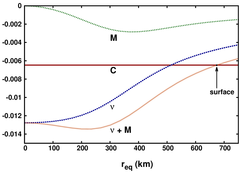
Figure 3: Behaviour of the different terms of the equation of motion as a function of the equatorial coordinate radius for the same star as shown in Fig. 1.

As already discussed in Ref. Cardall et al. (2001), the direction of the magnetic forces in the equatorial plane depends on the current distribution inside the star. In addition, the magnetic field changes its direction in the equatorial plane and, therefore, the Lorenz force reverses the direction inside the star. In our case, this can be seen from the qualitatively change in behaviour of the function $M(r,\theta)$ around $\rm{r_{eq}}\sim$ 350 km in Fig. 3.

In order to compare our results with those in the literature, we compute the mass-radius diagram for magnetized white dwarfs as shown in Fig. 4.

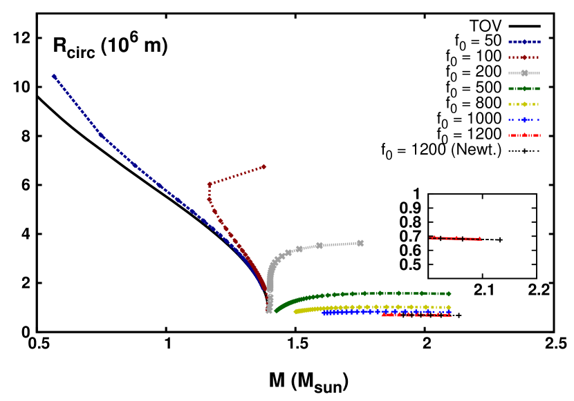
Figure 4: Mass-radius diagram for magnetized white dwarfs. Different curves represent different values of the current function $f_{0}$. We also compare the maximum white dwarf mass obtained in the Newtonian case (in black) and in the relativistic one (in red) for the maximum electric current value for which numerical convergence is achieved. This diagram is quite similar to the MR diagram calculated in Ref. Bera and Bhattacharya (2014). However, those authors have evaluated only Newtonian white dwarfs. All curves in this figure were calculated for a ratio between the magnetic and the matter pressure less than or quite close to 1 at the center of the star.

As pointed out in Ref. Paret et al. (2015), a fully consistent equilibrium configuration for magnetized white dwarfs is still lacking. Those same authors have used a relativistic framework with cylindrical coordinates and the splitting of the pressure into parallel and perpendicular components to show that the maximum magnetic field inside these objects can not exceed $\rm{1.5\times 10^{13}}\,$ G. Their solutions also indicate that it is not possible to have stable magnetized WDs with super-Chandrasekhar masses. The maximum magnetic field strength obtained in Ref. Paret et al. (2015) is less than the value obtained by a self-consistent solution of Newtonian white dwarfs as presented in Ref. Bera and Bhattacharya (2014), and orders of magnitude less than predicted in Ref. Das and Mukhopadhyay (2012). However, as shown in Refs. Coelho et al. (2014); Nityananda and Konar (2015); Chamel et al. (2013), the work Das and Mukhopadhyay (2012) has been criticized above all because their calculation violate both macro/micro physics properties essential for the stability of these objects.

In Fig. 4, the maximum white dwarf masses are obtained when the ratio between the magnetic and the matter pressure at the center of the star is less than or about 1. For such a strong magnetic field, the magnetic force has pushed the matter off-center and a topological change to a toroidal configuration can take place Cardall et al. (2001). This gives a limit for the magnetic field strength that can be computed within this approach, since our current numerical tools do not enable us to handle toroidal configuration.

The maximum masses of white dwarfs increase with the magnetic field. In our calculation, we found a relativistic white dwarf mass of 2.09 $\rm{M_{\odot}}$ for almost the same magnetic field strength at the center, B $\sim\rm{10^{14}}\,$ G, as in Ref. Bera and Bhattacharya (2014). The same authors presented configurations with magnetic fields up to $\rm{10^{16}\,G}$, which we have not found in our calculations. In the Newtonian case, we found a mass of 2.13 $\rm{M_{\odot}}$ for the most massive magnetized white dwarf. In both cases, the masses are well above the Chandrasekhar limit of 1.4 $\rm{M_{\odot}}$.

IV Rotating magnetized white dwarfs

Aside magnetic fields, rotation is a crucial observable in stellar astrophysics. In the case of neutron stars, for example, the magnetic dipole model states a direct relation between the rotation period/period derivative with the polar magnetic field of the star. For white dwarfs the interest in understanding these objects has been increasing with the years. Some observed white dwarfs rotate with periods of days or even years. One of the fastest observed WD possesses a spin period of $13.2\,s$ Mereghetti et al. (2009), a value similar to those observed in Soft Gamma Repeaters (SGRs) and Anomalous X-ray pulsars (AXPs), known as magnetars Duncan and Thompson (1992); Thompson and Duncan (1993). A relation between white dwarfs and magnetars was addressed in Ref. Malheiro and Coelho (2015), where the authors speculated that SGRs and AXPs with low magnetic field on the surface might be rotating magnetized white dwarfs.

Rigidly rotating non-magnetized white dwarfs were already studied long time ago in the Newtoninan framework as in Refs. Krishan and Kushwaha (1963); Anand (1965); James (1964); Roxburgh and Durney (1966); Monaghan (1966); Geroyannis and Hadjopoulos (1989) . In addition, the structure of rapidly rotating white dwarfs was performed in general relativity as in Ref. Arutyunyan et al. (1971), and more recently in Ref. Boshkayev et al. (2013), where the authors used the Hartle’s formalism Hartle (1967) to solve the Einstein equations. From the standpoint of rotation, it is clear that all rotating stars have to satisfy the mass-shedding, or Keplerian limit, as a condition of stability. This limit is reached when the centrifugal force due to the rotation does not balance gravity anymore and the star starts to lose particles from the equator, defining an upper limit to the angular velocity of uniformly rotating stars.

In the same way that rotation provides a natural limit for the stability of stars, in the case of WDs, there are also microphysics aspects, as for example, the inverse $\beta-$decay and pycnonuclear fusion reactions Chamel et al. (2013); Chamel and Fantina (2015); Coelho et al. (2014), that need to be taken into account for a complete and self-consistent description of these stars. In this paper, however, we restrict ourselves to the study of the combined effect of rotation and magnetic fields on the global structure of WDs and we do not address here the microphysics aspects.

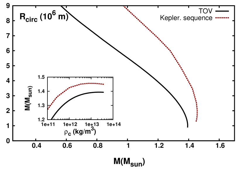
Figure 5: Mass-radius diagram for static and rotating white dwarfs. The TOV solution is shown in black, and in red (dashed) we show the Keplerian sequence for rotating WDs. On the bottom left-hand corner we show the gravitational mass as a function of the central density for the same sequence of stars.

In Fig. 5, we show the Tolman-Oppenheimer-Volkoff (TOV) solution for the structure of a spherically symmetric white dwarf and the mass-shedding frequency limit. The centrifugal force exerted by the rotation acts against gravity, which allows the star to support higher masses compared to the static case. In the first place, by comparison of Fig. 4 and Fig. 5, one sees that magnetic fields are more efficient than rotation in increasing the maximum mass of stars. The maximum mass obtained for a relativistic and magnetic white dwarf is 2.09 $\rm{M_{\odot}}$, whereas the maximum mass achieved by rotation is $\sim$1.45$\,\rm{M_{\odot}}$.

In Fig. 6, we show the relation between the Keplerian frequency ($f_{K}$) and the central density of the star. The higher angular velocity, the higher centrifugal forces, which pushes the matter outward, and therefore, acting against gravity. As a result, the stars are allowed to have more mass and, then, increasing the central density. This is possible, because the centrifugal forces due to rotation ($f_{c}\propto r\Omega^{2}$) have much more effect on the outer layers of the star. On the other hand, for non-rotating magnetized stars, the Lorenz force acts mainly in the inner layers of the star, reducing, and not increasing, the central densities in these objects as shown in Ref. Franzon et al. (2015).

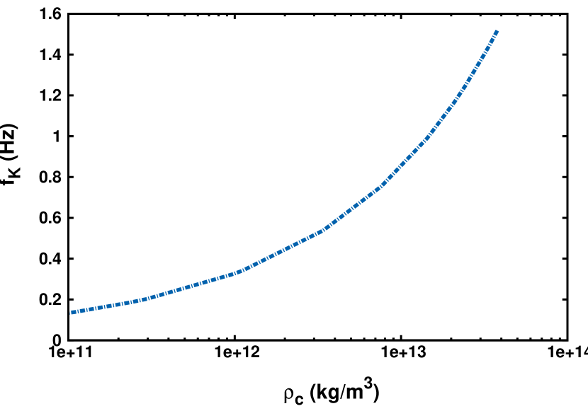
Figure 6: Keplerian frequency as a function of the central baryon density for the sequence as shown in Fig. 5. The maximum frequency reached by a non-magnetized and uniformilly rotating white dwarf is 1.52 $\rm{Hz}$.

Henceforth we will investigate the role played by the magnetic field in uniformly rotating white dwarfs . For a star with central enthalpy of $H_{c}=0.005\,c^{2}$, whose mass is close to the maximum mass in the static case, we present results of three different calculations: $A)$ static and non$-$magnetized; $B)$ rotating (with the Keplerian frequency) and non-magnetized and $C)$ rotating (with the Keplerian frequency) and magnetized. The cases $A)$ and $B)$ are presented in the mass-radius diagram in Fig. 4 and 5. For the case $B)$, the star rotates with its Keplerian frequency of 0.99 $\rm{Hz}$. In addition, to construct the models $C)$, we turn on the magnetic field until that the limit of numerical convergence is reached. The resulting magnetic field lines and the electric isopotential lines $A_{t}=$ const are depicted in Fig. 7.

Figure 7: Magnetic field lines (up) and electromagnetic potential lines (down) for a star with $H_{c}=0.005\,c^{2}$ and graviational mass of $\sim$1.57 $\rm{M_{\odot}}$, with a Keplerian frequency of 1.13 $\rm{Hz}$. The dipole magnetic moment reaches 6.93$\times 10^{33}\,\rm{Am^{2}}$ and the magnetic field intensity at the center of this white dwarf is 1.87 $\times 10^{14}\,$G.

In order to study how the Keplerian frequency changes with the magnetic field, we perform a calculation for different current functions $f=f_{0}=const$, from zero (case $B)$ to the maximum value of the magnetic field as shown in Fig. 7. As a result, the Keplerian frequency increases with the magnetic field as shown in Fig. 8. In this way, equilibrium configurations are obtained for higher centrifugal forces and, therefore, if the star can rotate faster, it can support higher masses, which explains the behaviour observed in Fig. 9.

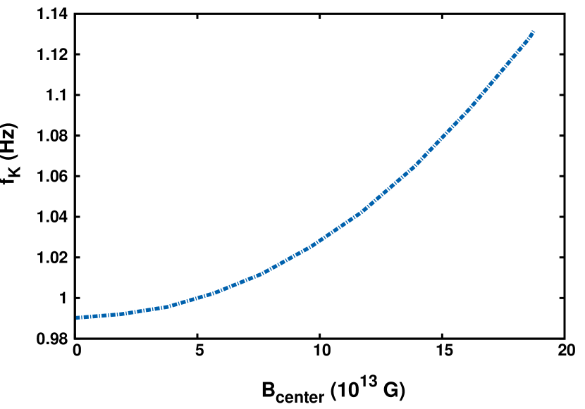
Figure 8: Keplerian frequency as function of the central magnetic field for non-magnetized (case $B$, i.e., $f_{K}$ = 0.99 $\rm{Hz}$) and magnetized (case $C$, i.e., $f_{K}$ = 1.13 $\rm{Hz}$) white dwarfs.

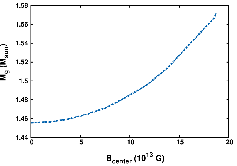
Figure 9: Gravitational mass as a function of the central magnetic field for a star with central enthalpy $H_{c}=0.005\,c^{2}$ for the cases $B)$ and $C)$, which are the same stars as shown in Fig. 8.

According to Figure 6, non-magnetized white dwarfs can reach a maximum Keplerian frequency of 1.52 $\rm{Hz}$. However, in the magnetic case (Fig. 8), the maximum Keplerian frequency is reduced to 1.13 $\rm{Hz}$, which corresponds to a white dwarf with gravitational mass of $\sim$ 1.57 $\rm{M_{\odot}}$ and a central magnetic field of 1.87 $\times 10^{14}\,$G.

V Conclusions

We computed perfect-fluid magnetized white dwarfs in general relativity by solving the coupled Einstein-Maxwell equations. We have applied a formalism that was developed for neutron stars to rotating magnetized white dwarfs. In our case, the equilibrium solutions are axisymmetric and stationary, with white dwarfs endowed with a strong poloidal magnetic field.

The observation of super-luminous Ia supernovae suggests that their progenitors are super-Chandrasekhar white dwarfs, whose masses are higher than 1.4 $\rm{M_{\odot}}$. The increasing in the mass may be a result from ultra-strong magnetic field inside the white dwarfs. The relevance of magnetic fields in enhancing the maximum mass of a white dwarf were studied and the results were obtained in a fully relativistic framework. We have shown that white dwarfs masses increase up to 2.09 $\rm{M_{\odot}}$ for a maximum magnetic field strength of $\sim 10^{15}\,$G in the stellar center. Thus, magnetic fields can, potentially, be responsible for super massive white dwarfs.

The structure of relativistic, axisymmetric and uniformly rotating magnetized white dwarfs were investigated self-consistently and all effects of electromagnetic field on the star equilibrium were taken into account. As usual, non-magnetized configurations at the mass shedding limit support higher masses as their static counterparts. However, we have seen that the magnetic field is much more efficient in increasing the mass of WDs than rotation. For example, the Keplerian sequence has a maximum mass of $\sim$ 1.45 $\rm{M_{\odot}}$, whereas for the maximum magnetic field configuration achieved in this calculation, the maximum mass of relativistic WDs is 2.09 $\rm{M_{\odot}}$, i.e., 33 $\%$ larger than the Chandrasekhar limit, and 2.13 $\rm{M_{\odot}}$ in the Newtonian framework.

We have also shown the increasing of the Keplerian frequency ($f_{K}$) with the magnetic field. The higher the magnetic field, the higher the Lorenz force, which, in turn, helps the star to support more mass than in the non-magnetized case. As a result, if these stars are more massive, they can rotate faster (see Fig. 8 and Fig. 9). In this case, the maximum mass obtained for rotating magnetized white dwarfs is of $\sim$1.57 $\rm{M_{\odot}}$, with a Keplerian frequence of 1.13 $\rm{Hz}$.

It is to be noted that purely poloidal or purely toroidal magnetic field configurations undergo intrinsic instabilities as suggested years ago in Refs. Markey and Tayler (1973); Tayler (1973); Wright (1973); Flowers and Ruderman (1977). The nature of this instability was confirmed both in Newtonian numerical simulations as in Refs. Lander and Jones (2012); Braithwaite (2006); Braithwaite and Nordlund (2006); Braithwaite (2007) and in general relativity framework as in Refs. Ciolfi and Rezzolla (2013); Lasky et al. (2011); Marchant et al. (2011); Mitchell et al. (2015). Analytical and numerical calculations have also shown that stable equilibrium configurations are obtained for magnetic fields composed not only by a poloidal component, which extends throughout the star and to the exterior, but also a toroidal one, which is confined inside the star  Armaza et al. (2015); Prendergast (1956); Braithwaite and Spruit (2004); Braithwaite and Nordlund (2006); Akgün et al. (2013). In addition, the magnetic field might decay due to ohmic effects and, therefore, changing its strength and distribution in the star Goldreich and Reisenegger (1992). Although we model magnetized white dwarfs with a purely poloidal magnetic field components, which are not the most general case, we have shown, in a fully general relativity way, that these stars can considerably increase their masses due to magnetic field effects and, therefore, contributing to super-luminous SNIa. In a future work, in order to have a more complete description of the stars presented here, we intend to take into account magnetic field configurations with both poloidal and toroidal components, a B-field dependent equation of state and effects of the anomalous magnetic moment, too.