Edge structure of graphene monolayers in the $\nu=0$ quantum Hall state

Abstract

Monolayer graphene at neutrality in the quantum Hall regime has many competing ground states with various types of ordering. The outcome of this competition is modified by the presence of the sample boundaries. In this paper we use a Hartree-Fock treatment of the electronic correlations allowing for space-dependent ordering. The armchair edge influence is modeled by a simple perturbative effective magnetic field in valley space. We find that all phases found in the bulk of the sample, ferromagnetic, canted antiferromagnetic, charge-density wave and Kekulé distortion are smoothly connected to a Kekulé-distorted edge. The single-particle excitations are computed taking into account the spatial variation of the order parameters. An eventual metal-insulator transition as a function of the Zeeman energy is not simply related to the type of bulk order.

I introduction

When subjected to a strong perpendicular magnetic field, the electrons confined to the two-dimensional (2D) carbon lattice of graphene form a unique quantum Hall (QH) system. Notably graphene at neutrality is an example of QH ferromagnetism with many competing ground states MacDonald06 ; Herbut1 ; Herbut2 ; Alicea ; Yang et al. (2006); Jung and MacDonald (2009); Kharitonov (2012a); Abanin et al. (2013); Sodemann and MacDonald (2014). In such systems we expect generically complex physics at the edge. Early work on graphene edge states Abanin et al. (2006) has shown that when taking into account the electron spin degree of freedom, the edge states should be of helical nature, i.e., exhibiting counterpropagating modes carrying opposite spin polarizations. Graphene was thus proposed to be a model candidate for a quantum spin Hall (QSH) system. Furthermore, graphene has unique features so that it may be an ideal probe material to study QH edge physics experimentally : in semiconductor-based 2D electron gas systems the confining potential is soft at the scale of the magnetic length so that there may be edge reconstruction Chklovskii et al. (1992); Chamon and Wen (1994); Yang (2003), spoiling the ideal theoretical description. Therefore, the understanding of edge phenomena in these 2D systems is difficult Chang et al. (1996); Grayson et al. (1998) and still controversial. In contrast, the boundaries of the graphene lattice are directly defined at the atomic level. Therefore, they naturally represent atomically sharp QH edges. This should allow observation of QH edge state physics without complications from edge reconstruction Bhatt ; Li et al. (2013). The fabrication, design, and control of graphene edge structures with atomic level precision is a field of ongoing research : see, e.g., Refs. Fuhrer, 2010; Cai et al., 2010; Huang et al., 2012. Among the theoretical approaches, also a mean-field treatment of a Hubbard-type model has been applied to the edge physics Lado_noncollinear_2014 . The QSH nature of the graphene edge has been the subject of recent experimental investigations Young et al. (2014). At Landau level filling factor $\nu=0$, upon tilting the applied magnetic field with respect to the graphene sheet, there is a metal-insulator transition for some critical angle. This suggests a change of the bulk state as a function of tilting. Indeed, extensive theoretical studies of the $\nu=0$ ground state (GS) structure of bulk graphene Jung and MacDonald (2009); Kharitonov (2012a); roy1 ; roy2 have shown the existence of various competing phases with distinct symmetry-breaking properties. While the graphene GS at neutrality is a highly degenerate SU(4) ferromagnetic multiplet, small symmetry-breaking terms due to short-distance physics lift this degeneracy and the system may form various different phases. Among these phases are e.g. the ferromagnet (F) stateMacDonald06 ; Yang et al. (2006) or the antiferromagnet (AF) state, where the latter may form a canted antiferromagnetic (CAF) state as has been pointed out by Kharitonov in Ref. Kharitonov, 2012a. Further possible phases include a charge-density waveAlicea ; Alicea2 ; Fuchs ; Jung and MacDonald (2009) (CDW) or a Kekulé distorted stateNomura2 ; Hou (KD). Transitions between these states may be induced by varying the Zeeman energy which is done by tilting the field.

In this paper we study the edge structure of the $\nu=0$ QH state in the presence of SU(4)-symmetry-breaking interactions. We use a simple model of the edge potential in the basis of the $n=0$ LL orbitals appropriate to an armchair termination of the graphene lattice and treat interactions by a Hartree-Fock (HF) approximation. Our variational ansatz is orbital-dependent so it captures the spatial variations of the ordering from the bulk to the edge (an effect which is absent in previous HF studies Kharitonov (2012b)). We find that there is always a crossover towards a Kekulé distorted region close to the edge. There is appearance also of spin/valley nontrivial entanglement which is limited to the transition region towards Kekulé order and does not take place either in the bulk or close to the edge. We propose a quantitative measurement of the entanglement by computing the concurrence as a function of edge distance. Within HF we also compute the single-particle properties of the particle-hole excitation spectrum. We discuss how this spectrum varies with the edge distance and also how it is influenced by the nature of the bulk order. Our main finding is that there should be always a metal-insulator transition as a function of the Zeeman field whatever the nature of the ordered phase. So strictly speaking the experimental observations of Ref. Young et al., 2014 do not imply that their graphene bulk is a CAF state. It should be noted that our HF treatment has some shortcomings. Notably the Coulomb exchange interaction in the $n=0$ LL leads to a coupling between charge and spin/valley degrees of freedom. So in general charge motion is done through spin/valley textures as proposed in Refs. Brey and Fertig, 2006a; Brey and Fertig, 2006b; Fertig and Brey, 2006; Murthy et al., 2014. As in previous HF works Kharitonov (2012b) we will not try to model these effects. While the edge effects will overcome exchange energy close enough to boundary, they may change the nature of excitations right in the transition region. More work is needed to understand this point.

The paper is structured as follows : In Sec. II, we define the theoretical framework describing the $\nu=0$ QH state of graphene in the presence of a boundary and the corresponding model Hamiltonian. We introduce the parametrization of the Hartree-Fock (HF) GS wave function in Sec. III. In Sec. IV, we present results for the GS and its properties obtained from minimizing the HF energy functional. We describe the evolution of the different possible bulk phases when moving towards to the edge. We find that the presence of a boundary gives rise to novel spin/isospin configurations which do not exist in the bulk. Furthermore, we show the existence of an intermediate region between the bulk and the edge with nontrivial entanglement of spin and valley isospin. In Sec. V, we extend our HF treatment to compute the spatial evolution of the single particle (SP) energy levels and corresponding eigenstates from the bulk to the boundary. As pointed out by previous work (Kharitonov, 2012b), the SP spectra can either exhibit nonzero gaps or support gapless edge states, depending on the system parameters determining the bulk phase. We describe how the spatial variation of the spin/isospin texture influences the shape of the SP energy levels. This leads to an understanding of the edge gap, the number of conducting channels, as well as possible conclusions for the bulk symmetry properties drawn from the conductance behavior of the edges. In a final part, we compute the spin and isospin properties of the corresponding SP eigenstates to directly prove that the edge states of the $\nu=0$ QH state in graphene indeed exhibit the helical properties of a QSH state. Sec. VI finally discusses our results in relation to experimental findings and contains our conclusions.

II Model of the Graphene edge

We first recall basic facts about the electronic structure of graphene Castro Neto et al. (2009); Goerbig (2011). The hexagonal structure admits two triangular Bravais sublattices $A$ and $B$ that form the basis for a tight-binding Hamiltonian. In the Brillouin zone there are two special degeneracy points : at these Dirac points $K$ and $K^{\prime}$, the valence and the conductance band form Dirac cones and touch at the Fermi level for neutral graphene. In the vicinity of the Dirac points, for each orientation of the spin $\sigma=\uparrow,\downarrow,$ the electronic wave functions $\Psi_{A}$ and $\Psi_{B}$ on the two sublattices can be written as :

$$\Psi_{A{,\sigma}}(\mathbf{r}) =e^{i\mathbf{K}\cdot\mathbf{r}}\psi_{A{,\sigma}}+e^{-i\mathbf{K}^{\prime}\cdot\mathbf{r}}\psi_{A{,\sigma}}^{\prime},$$ (1a)

$$\Psi_{B{,\sigma}}(\mathbf{r}) =e^{i\mathbf{K}\cdot\mathbf{r}}\psi_{B{,\sigma}}+e^{-i\mathbf{K}^{\prime}\cdot\mathbf{r}}\psi_{B{,\sigma}}^{\prime}.$$ (1b)

Assembling the envelope functions in a four spinor notation we write for the electronic state :

$$\Psi_{{\sigma}}=\begin{pmatrix}\psi_{A{,\sigma}}\\ \psi_{B{,\sigma}}\\ \psi_{A{,\sigma}}^{\prime}\\ \psi_{B{,\sigma}}^{\prime}\end{pmatrix}_{{H_{K,K^{\prime}}\otimes H_{A,B}}},$$ (2)

where the subindex $H_{K,K^{\prime}}\otimes H_{A,B}$ indicates that the state $\Psi_{\sigma}$ lives in the Hilbert space formed as the direct product between Dirac valley space $H_{K,K^{\prime}}$ and the $A,B$ sublattice space $H_{A,B}$. An applied magnetic field leads to the formation of Landau levels (LL) with energies :

$$E_{n}=\frac{v_{F}}{\ell_{B}}\sqrt{2|n|}\;\text{sgn(}{n}\text{)},$$ (3)

where $n\in\mathbb{Z}$ is the LL index, $\ell_{B}=\sqrt{\frac{\hbar c}{eB_{\perp}}}$ is the magnetic length for perpendicular magnetic field strength $B_{\perp}$, and $v_{F}$ denotes the Fermi velocity. The corresponding eigenstates can be written as :

$$\Psi_{n\neq 0{,\sigma}}=\frac{1}{\sqrt{2}}\begin{pmatrix}|n-1\rangle\\ |n\rangle\\ -|n-1\rangle\\ -|n\rangle\end{pmatrix}_{{H_{K,K^{\prime}}\otimes H_{A,B}}},\hskip 10.0pt\Psi_{n=0{,\sigma}}=\begin{pmatrix}0\\ |0\rangle\\ 0\\ -|0\rangle\end{pmatrix}_{{H_{K,K^{\prime}}\otimes H_{A,B}}}.$$ (4)

The filling factor $\nu$ of the Landau levels is defined by :

$$\nu=\frac{n_{e}}{2\pi\ell^{2}_{B}},$$ (5)

where $n_{e}$ denotes the electronic density. The configuration of neutral graphene, i.e., $\nu=0$ is peculiar. Indeed this particle-hole symmetric situation corresponds to the case in which all the LLs with $n<0$ are filled and all the LLs with $n>0$ are empty, but the $n=0$ LL is exactly half filled with two electrons per orbital. The form of the $n=0$ wave function as given in Eq. (4) implies that $n=0$ LL electrons reside on one of the sub-lattices only. In the following, we consider the case of neutral graphene and therefore study the properties of electrons in the $n=0$ LL. We simplify the notation by collecting only the non-zero entries of the $n=0$ spinor in Eq. (4) as :

$$\Psi_{0}=\begin{pmatrix}|\uparrow+\rangle\\ |\uparrow-\rangle\\ |\downarrow+\rangle\\ |\downarrow-\rangle\end{pmatrix}_{{H}},$$ (6)

identifying the valley and the sublattice indices in a common valley-isospin $\tau$ as $\tau=+\mathrel{\hat{=}}K\leftrightarrow A$ and $\tau=-\mathrel{\hat{=}}K^{\prime}\leftrightarrow B$. In the four-dimensional Hilbert space $H=H_{spin}\otimes H_{valley}$ we use the indices $\mu,\nu$ to label the four possible configurations of spin and isospin in this space: $\mu,\nu\in\{\uparrow+,\uparrow-,\downarrow+,\downarrow-\}$. Due to the fourfold degeneracy in spin space ($\sigma=\uparrow,\downarrow$) and in valley space ($\tau=+,-$), integer QH effect in graphene is expected at values of $\nu$ that change in steps of four.

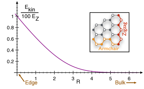
Figure 1: Shape of the kinetic energy edge potential $E_{kin}$ in $\mathcal{H}_{kin}$ of Eq. (8). The kinetic energy rises from $E_{kin}=0$ in the bulk (equivalent to the case of infinitely extended, translationally invariant graphene in the $n=0$ LL) to the energy of the $n=1$ LL exactly at the edge. The curve was obtained from solving the problem of free electrons on a graphene lattice in the presence of a magnetic field in the presence of boundary, i.e., by applying appropriate boundary conditions for an armchair edge (see inset). Zigzag edges have similar nonzero energy states but also additional zero-energy modes that are beoynd the scope of our work.

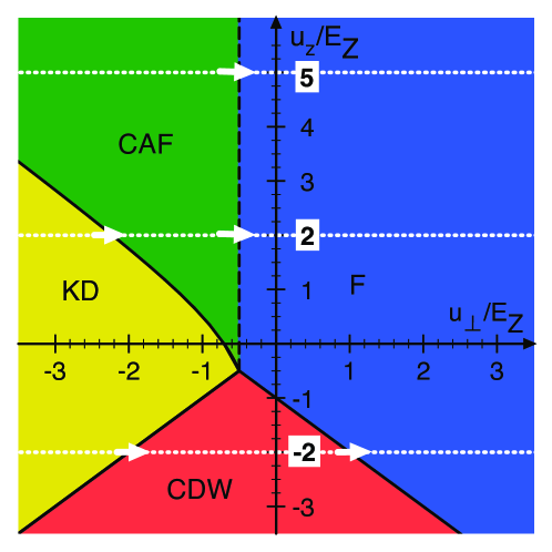
Figure 2: Bulk GS phase diagram as a function of the coupling energies $u_{\perp}$ and $u_{z}$ of the $\nu=0$ QH state for a Hamiltonian as in Eq. (7). Different colors distinguish between the different possible GS phases. The white, dotted lines indicate the parameters we choose throughout this paper to perform cuts through the phase diagram in order to explore the behavior of all possible GS phases when starting from the bulk and moving towards an edge of the graphene lattice. The phase diagram for the different GS phases in the bulk of graphene was first presented in Ref. Kharitonov, 2012a.

The total Hamiltonian we use is given by :

$$\mathcal{H}=\mathcal{H}_{kin}+\mathcal{H}_{Z}+\mathcal{H}_{Coul}+\mathcal{H}_{Aniso},$$ (7)

where we have a space dependent kinetic energy induced by the presence of the boundary :

$$\mathcal{H}_{kin}=-\sum_{i}E_{kin}(\mathbf{r}_{i})\mathbf{\tau}^{i}_{x},$$ (8)

where the index $i$ labels the positions of the electron orbits. The hexagonal graphene lattice can be terminated in many different ways, yielding several possible edge structures. Every different atomic configuration leads to different boundary conditions for the wavefunctionAkhmerov and Beenakker (2008). Two extreme cases are the so-called zigzag and armchair edges Brey and Fertig (2006a). A finite piece of graphene terminated by a zigzag edge and an armchair edge is shown in the inset of Fig. 1. The kinetic energy and the corresponding eigenstates can be obtained analytically Abanin et al. (2006); Brey and Fertig (2006b); Mei and Lee (1983); Janssen et al. (1994). This is equivalent to turning the level index into a space dependent quantity $n(R)$ where $R$ relates to the distance to the edge $r$ as $r=R{\ell_{B}}/{\sqrt{2}}$. In Fig. 1 we show the spatial shape of the kinetic energy $E_{kin}$ obtained by this procedure, as we will use it in the subsequent calculations. We write the kinetic energy as a space-dependent potential proportional to $\tau_{x}$ (a comparable treatment can be found in Refs. Kharitonov, 2012b; Murthy et al., 2014). This corresponds to a perturbative treatment as it assumes an expansion of the perturbed edge states in terms of the unperturbed bulk basis states. It restricts our description to the case of ”armchair-like” boundaries : one can always infer the number of branches in the SP edge spectrum as being equal to the number of degenerate SP levels in the bulk and hence apply a perturbative expansion as implied by Eq. (8). A derivation of such a Hamiltonian describing the kinetic potential of a graphene edge using arguments of perturbation theory can be found in Ref. Kharitonov, 2012b. The edges terminated by a zigzag boundary condition support dispersionless surface states Brey and Fertig (2006a); Brey and Fertig (2006b) that break the simple bulk/edge correspondence. They are beyond our simple treatment. The form of the kinetic energy in Eq. (8) is valid only in the regime $E_{kin}\ll\hbar\omega_{c}$, i.e., spatially not too close to the edge. As can be seen from Fig. 1, this condition is very well met if we restrict the subsequent discussion to the regime $R>3$. Hence the restriction $R>3$ corresponds to a minimal distance $r_{min}\approx 2.12\ell_{B}$, which at realistic experimental values corresponds to $r_{min}\approx 120\text{a}_{0}$, where $\text{a}_{0}$ denotes the lattice constant of graphene. The Zeeman energy can be written as :

$$\mathcal{H}_{Z}=-E_{Z}\sum_{i}\mathbf{\sigma}^{i}_{z}.$$ (9)

In the case of graphene the spacing between kinetic LL energy levels, $\Delta E_{kin}$, easily exceeds the Zeeman energy by two orders of magnitude. The Coulomb interaction is given by :

$$\mathcal{H}_{Coul}=\frac{1}{2}\sum_{i\neq j}\frac{e^{2}}{\varepsilon}\frac{1}{|\mathbf{r}_{i}-\mathbf{r}_{j}|},$$ (10)

where $\varepsilon$ is an effective dielectric constant which depends upon the substrateSantos and Kaxiras (2013). It has full SU(4) symmetry. At neutrality we have an example of quantum Hall ferromagnetism MacDonald06 with this large symmetry : the ground state is thus highly degenerate and forms an irreducible representation of SU(4). However this symmetry is only approximate. In fact it is weakly broken by lattice-scale effects that include short-range Coulomb interactions and electron-phonon couplings. It is difficult to obtain precise estimates of these effects but their symmetry-breaking properties can be encoded in the following Hamiltonian :

$$\mathcal{H}_{Aniso}=\frac{1}{2}\sum_{i\neq j}\,\left[g_{x}\tau_{x}^{i}\tau_{x}^{j}+g_{y}\tau_{y}^{i}\tau_{y}^{j}+g_{z}\tau_{z}^{i}\tau_{z}^{j}\right]\,\,\delta^{2}(\mathbf{r}_{i}-\mathbf{r}_{j}),$$ (11)

with $\delta$ denoting the Dirac delta function. This Hamiltonian $\mathcal{H}_{Aniso}$ has been proposed by Aleiner et al. Aleiner et al. (2007) and its effects have been analyzed at the mean-field level by KharitonovKharitonov (2012a). Its symmetry properties and phase diagram have been studied by exact diagonalization Wu14 . It is parametrized by the coupling constants $g_{x,y,z}$ whose values are not known with precision. It is likely that the ratio of the energy scales between Coulomb interaction and these anisotropies is of the order of $10^{2}$. It is thus best to explore the complete phase diagram taking these parameters as unknowns. For monolayer and bilayer graphene at neutrality, there is a rich phase diagram as a function of these couplings Kharitonov (2012a, c). The fractional quantum Hall states are also sensitive to these effects Sodemann and MacDonald (2014).

We now perform a HF study of this Hamiltonian by including the edge potential. We note that in this approach we neglect all possible spatial dependence of the coupling constants, which is justified as long as we analyze a spatial domain not too close to the edge.

III Hartree-Fock treatment

The neutral $\nu=0$ state corresponds to the half-filled case where two of the four available states per orbital are occupied. We look for the ground state within the family of Slater determinants of the form :

$$|G\rangle=\prod_{p}\left(\sum_{\mu,\nu}\,g_{\mu\nu}\,c_{\mu}^{\dagger}(p)c_{\nu}^{\dagger}(p)\right)\,|0\rangle,$$ (12)

where $p$ denotes the Landau-gauge momentum component along the edge which labels the electron orbitals. The vacuum $|0\rangle$ consists of the completely occupied set of states for all $n<0$ and completely empty states for all $n>0$. In Eq. (12) ${{g}}$ is a 4 by 4 antisymmetric matrix, i.e., $g_{\mu\nu}=-g_{\nu\mu}$, in order to describe a valid fermionic state and $\text{Tr}[gg^{\dagger}]=2$ to ensure normalization of the two-particle state. We minimize the energy of the Slater determinant by varying $g$. To capture the effect of the edge potential we take the $g$ matrix to be momentum dependent, i.e., $g\equiv g(p)$ in Eq. (12). Due to the duality between the longitudinal momentum $p$ and the transverse coordinate $r_{p}=p\ell^{2}_{B}$ this is equivalent to a space dependent description of the problem. The most general antisymmetric matrix ${{g}}$ has 12 real parameters. By exploiting the symmetry properties of the state $|G\rangle$ and the Hamiltonian, one can reduce the number of free parameters. We use the same strategy as in Ref. Ezawa et al., 2005 where an equivalent problem was studied in the context of electronic bilayer systems. It is convenient to rewrite the problem in terms of the following simple expectation values :

$$S_{\alpha} =\frac{1}{2}\langle G|\text{c}^{\dagger}(p)\mathbf{\sigma}_{\alpha}\,\text{c}(p)|G\rangle=\frac{1}{2}\text{Tr}[\sigma_{\alpha}gg^{\dagger}],$$ (13a)

$$T_{\alpha} =\frac{1}{2}\langle G|\text{c}^{\dagger}(p)\mathbf{\tau}_{\alpha}\text{c}(p)|G\rangle=\frac{1}{2}\text{Tr}[\tau_{\alpha}gg^{\dagger}],$$ (13b)

$$R_{\alpha\beta} =\frac{1}{2}\langle G|\text{c}^{\dagger}(p)\mathbf{\sigma}_{\alpha}\mathbf{\tau}_{\beta}\text{c}(p)|G\rangle=\frac{1}{2}\text{Tr}[\sigma_{\alpha}\tau_{\beta}gg^{\dagger}].$$ (13c)

The expressions of Eqs. (13a) and (13b) yield the components of the total spin $S_{\alpha}$ and isospin $T_{\alpha}$ per orbital $p$. The energy contribution from the symmetry breaking interaction Hamiltonian of Eq. (11) is now given by :

$$\langle G|\mathcal{H}_{Aniso}|G\rangle=\frac{1}{2}\sum_{\alpha}u_{\alpha}\Big{(}\text{Tr}[\tau_{\alpha}gg^{\dagger}]^{2}-\text{Tr}[\tau_{\alpha}gg^{\dagger}\tau_{\alpha}gg^{\dagger}]\Big{)},$$ (14)

where the anisotropy energies $u_{\alpha}$ are given by $u_{\alpha}=\frac{g_{\alpha}}{2\pi\ell_{B}^{2}}$. Isotropy of the interaction potential in the $x$-$y$-plane implies that $u_{x}=u_{y}=:u_{\perp}$. Using Eqs. (13) and (14), we obtain the following expression for the functional of the total energy $E_{tot}=\langle G|\mathcal{H}|G\rangle$ :

$$E_{tot}=-2E_{kin}\,T_{x}-2E_{Z}\,S_{z}+\sum_{\alpha}u_{\alpha}\Big{(}T_{\alpha}^{2}-\sum_{i}R^{2}_{i\alpha}-\mathbf{S}^{2}\Big{)}.$$ (15)

The $12-2=10$ free parameters of the problem (dropping the overall phase and normalization constant) are now encoded in the 6 components of the total spin $\mathbf{S}$ and the total isospin $\mathbf{T}$, together with 4 out of 9 components of $R_{\alpha\beta}$ which can be chosen independently. The invariance of $E_{tot}$ in Eq. (15) under rotations of $\mathbf{S}$ in spin space and rotations of $\mathbf{T}$ around the $z$-axis in isospin space allows us to choose $S_{y}=S_{x}=T_{y}=0$ with no loss of generality, yielding seven variables to be determined. The dimension of parameter space can be further reduced by careful consideration of all the symmetries of the problem. As demonstrated by Ezawa et al. Ezawa et al. (2005) in a situation of an equivalent symmetry class, reduction is possible to a total number of three free parameters. For the present system, this leads us to a minimization problem for the total energy $E_{tot}$ with respect to the variational parameters $-1\leq\alpha\leq 1,-1\leq\beta\leq 1$, and $\chi\in\mathbb{R}$, which are related to observables of Eq. (13) by :

$$S_{z}=\frac{1}{\sqrt{1+\chi^{2}}}\,\sqrt{1-\alpha^{2}},\quad T_{x}=\frac{\chi}{\sqrt{1+\chi^{2}}}\,\alpha\sqrt{1-\beta^{2}},\quad T_{z}=\frac{\chi}{\sqrt{1+\chi^{2}}}\,\alpha\beta,$$ (16)

and

$$\sum_{i}R^{2}_{ix}=\frac{T_{z}^{2}}{\chi^{2}},\quad\sum_{i}R^{2}_{iy}=\chi^{2}\mathbf{S}^{2},\quad\sum_{i}R^{2}_{iz}=\frac{T_{x}^{2}}{\chi^{2}},$$ (17)

where the index $i$ runs over the spatial components $\{x,y,z\}$. The density matrix $\rho_{g}=gg^{\dagger}$ is connected to these quantities as (summation convention implied) :

$$\rho_{g}=\frac{1}{2}\mathbb{1}+\frac{1}{2}\Big{(}\sigma_{i}\,S_{i}+\tau_{i}\,T_{i}+\sigma_{i}\tau_{j}\,R_{ij}\Big{)}.$$ (18)

IV Ground state properties

IV.1 Evolution of the Spin-Isospin Texture close to the Edge

The bulk GS of graphene within the model we use has several different phases depending on the anisotropy energies $u_{\perp}$ and $u_{z}$ compared to the Zeeman energy $E_{Z}$Kharitonov (2012a); Wu14 . The anisotropies $u_{\perp},u_{z}$ and the Zeeman term $E_{Z}$ select some subset of the manifold of SU(4) ferromagnetic ground states. These phases have distinct spin and isospin configurations, i.e., by different spin textures. The mean-field GS diagram is shown in Fig. 2. It is correct beyond mean-field as shown by exact diagonalization techniques Wu14 . Notably all these bulk phases do not involve spin/valley entanglement. We now generalize the description of these phases by treating the effect of a boundary of the lattice. We proceed as follows : we minimize the energy $E_{tot}(\alpha,\beta,\chi)$ of Eq. (15), including a space dependent edge potential of the shape shown in Fig. 1 by varying the parameters $\alpha,\beta,\chi$. Then from the knowledge of the parameters $\alpha(R),\beta(R),\chi(R)$, we can compute the values of the observables $S_{z}(R),T_{x}(R),T_{z}(R)$ of the GS $|G\rangle$ via Eq. (16). It is also possible to construct the entire density matrix $\rho_{g}$ characterizing the GS via Eq. (18).

In order to obtain a full picture capturing the edge behavior of all possible bulk phases shown in Fig. 2, our choice of system parameters is guided by the following idea : for fixed Zeeman energy $E_{Z}$, we vary the coupling energies $u_{\perp}$ and $u_{z}$ because this can be realized experimentally by tilting the magnetic field. We choose three values of the perpendicular coupling energy $u_{z}$ : $u_{z}=5E_{Z},\;u_{z}=2E_{Z}$ and $u_{z}=-2E_{Z}$, and we vary the perpendicular coupling in the range $-3E_{Z}\leq u_{\perp}\leq 3E_{Z}$. This leads to horizontal cuts through the $\nu=0$ GS phase diagram in the $u_{\perp},u_{z}$-plane, shown by white dotted lines in the phase diagram of Fig. 1. For $u_{z}=5E_{Z}$ and $u_{z}=2E_{Z}$ by varying $u_{\perp}$ we meet the KD, CAF and F phases :

For $u_{z}=-2E_{Z}$ and varying again $u_{\perp}$ we find the KD, CDW and F phases :

The corresponding bulk phase transitions are indicated by white arrows in the phase diagram in Fig. 1.

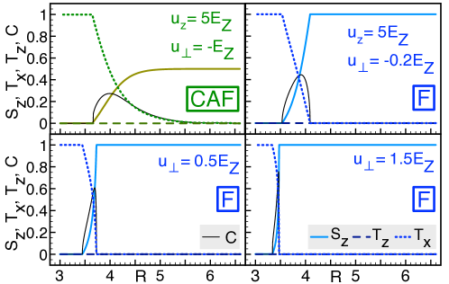
Figure 3: Evolution of the spin and isospin as well as the concurrence $C$ as functions of $R=\sqrt{2}r/\ell_{B}$, with $r$ the distance from the edge. We fix $u_{z}=5\,E_{Z}$ and vary $u_{\perp}$. (Colored lines: $S_{z}$, solid; $T_{z}$, dashed; $T_{x}$, dotted. Black, thin, solid line: Concurrence $C$). There is a transition between the bulk phase on the right-hand side [CAF for $u_{\perp}=-E_{Z}$ in the upper left panel (green colors) and F for all other choices of $u_{\perp}$ shown (blue colors)] to a KD phase at the edge. In an intermediate regime spin and isospin, are canted with $0<S_{z}<1$ and $0<T_{x}<0$ at the same time and nonzero values of the concurrence. With growing $u_{\perp}$, this domain wall grows narrower in space and moves closer to the boundary.

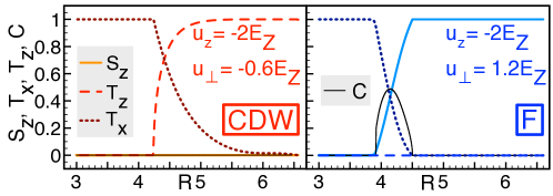
Figure 4: Same as Fig. 3 for transverse coupling energy $u_{z}=-2E_{Z}$ and different perpendicular coupling energies $u_{\perp}$, such that the phases of the lower half plane of the GS phase diagram are established in the bulk. Left panel: $u_{\perp}=0.6$, leading to a CDW in the bulk (red colors). Right panel: $u_{\perp}=1.2E_{Z}$, at which the bulk is in a F phase (blue colors).

We first investigate the influence of the edge potential on the spin and isospin observables $\mathbf{S}$ and $\mathbf{T}$. More precisely, we discuss the spatial evolution of the components $S_{z}(R),T_{x}(R),T_{z}(R)$ for different choices of the anisotropy energies $u_{\perp}$ and $u_{z}$ compared to the Zeeman energy $E_{Z}$. Figure 3 shows the results for $u_{z}=5E_{Z}$, corresponding to a cut through the upper half plane (we plot obsevables with colored lines). The four different panels depict the situation for different values of $u_{\perp}$ : for $u_{\perp}=-E_{Z}$, the bulk system is in the CAF phase with canting angle $\cos{\theta}=S_{z}=1/2$ (upper left panel), whereas for $u_{\perp}=-0.2E_{Z}$, $u_{\perp}=0.5E_{Z}$, and $u_{\perp}=1.5E_{Z}$ the bulk system establishes a F phase in which the spins are fully polarized. The colored curves shown in Fig. 4 correspond to the obervables for a cut through the lower half plane of the phase diagram at $u_{z}=-2E_{Z}$. Here, the perpendicular couplings are chosen so that the left panel at $u_{\perp}=-0.6E_{Z}$ corresponds to a CDW phase whereas the right panel at $u_{\perp}=1.2E_{Z}$ again corresponds to a F bulk phase, as predicted by the GS phase diagram of Fig. 2. Curves for values of the anisotropy energies favoring a KD phase in the bulk are not shown since in this case the system does not undergo any transition whatsoever but remains in the bulk KD phase all the way to the edge.

In general, one can distinguish three different regimes for the behavior of the observables as a function of the distance $r=\frac{\ell_{B}}{\sqrt{2}}R$ to the edge. For sufficiently large values of $R$, i.e., deep enough in the bulk, we recover the results of mean-field theory Kharitonov (2012a). Close enough to the edge, the system is driven into a KD phase with $N_{x}=1$ and $S_{z}=N_{z}=0$, independently of the bulk phase it adopts. This behavior is due to the edge potential in the kinetic energy Hamiltonian $\mathcal{H}_{kin}$ in Eq. (8) : this term is proportional to $\tau_{x}$, so it acts as a Zeeman effect in isospin space, polarizing the isospin along the $x$-direction as soon as $E_{kin}(R)$ is large enough. This behavior is also consistent with previous works Fertig and Brey (2006); Murthy et al. (2014). In an intermediate regime we find a finite interval in space in which $S_{z}\neq 1,\,T_{x}\neq 1$ and $T_{z}\neq 0,\,N_{x}\neq 0$, i.e., the spin and the isospin are canted simultaneously with respect to their bulk values. There is thus a domain wall at a small finite distance from the edge. For the CAF configuration, this domain wall connects smoothly to the bulk configuration. For a system in a F phase in the bulk however, the change in spin and isospin is abrupt and the domain wall is narrower with increasing $u_{\perp}$. Hence, for larger values of $u_{\perp}$, the F phase of the bulk proves to be more resistant against the increasing influence of the edge.

From our analysis and the results shown in Figs. 3 and 4 we therefore draw the following conclusions: The phases in the bulk of a finite sample of graphene do not remain unaffected close enough to the edges. Indeed the effective edge potential causes the bulk state to undergo a transition in which the polarizations of spin and isospin change simultaneously. Sufficiently close to the edge, the GS is driven into a KD phase independently of the nature of the bulk phase.

IV.2 Spin-Valley Entanglement of Edge States

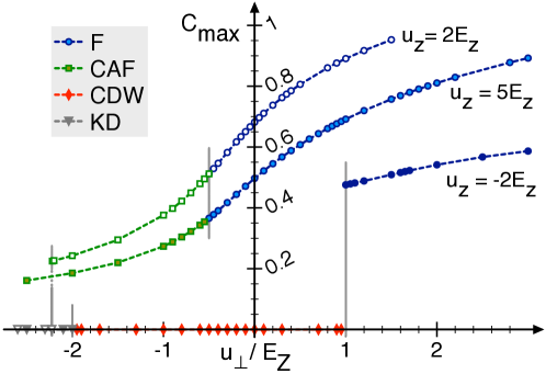
Figure 5: Maximum concurrence $C_{max}$ in the different regimes from the bulk to the edge. For three different values of the coupling energy $u_{z}$, we vary $u_{\perp}$. Different symbols represent different phases in the bulk at the respective value of $u_{\perp}$: F (blue circles), CAF (green squares), CDW (red diamonds), and KD (gray triangles). Empty, shaded, or filled symbols distinguish between the cuts at different $u_{z}$. The dashed lines connect the data points as a guide to the eye. Vertical, gray lines mark the values of $\{u_{z},u_{\perp}\}$, at which, in the bulk, transitions between the respective phases occur. We observe that non-zero values of $C$ happen only if the system in the bulk is in a CAF or in a F phase. In this case, the CAF/F transition is smooth. If the bulk is CDW or KD,the concurrence remains equal to zero all the way from the bulk to the edge. This leads to a discontinuous jump in the curve of $C_{max}$ at the point of the CDW/F transition.

The parametrization of $\mathbf{S},\mathbf{T},$ and ${{\text{R}_{\alpha\beta}}}$ in terms of the three parameters $\alpha,\beta,$ and $\chi$ in Eqs. (16) and (17) allows for complete reconstruction of the density matrix $\rho_{g}$ via Eq. (18) using the values of the parameters obtained by minimizing $E_{tot}$ from Eq. (15). Therefore, we have a full description of the GS and its spatial evolution from the bulk towards the edge. In this paragraph we investigate the entanglement between spin and isospin degrees of freedom in the system. For the infinite bulk case, product states of the form $|s\rangle\otimes|n\rangle$, where $|s\rangle$ denotes the (single particle) spin state and $|n\rangle$ the (single particle) isospin state, have been used as an ansatz to minimize the GS energyKharitonov (2012a, c, b). Existing studies of edge states using a variational trial wave function approach have suggested Murthy et al. (2014), however, that for a non-zero edge potential, spin and isospin might not remain independent, separable observables, but become entangled. In order to quantify the amount of entanglement in the bipartite two-level system $H=H_{spin}\otimes H_{valley}$, we calculate the concurrence $C$ according to the definitionMintert et al. (2005) :

$$C=\text{max}(\lambda_{1}-\lambda_{2}-\lambda_{3}-\lambda_{4},0),$$ (19)

where the $\lambda_{i}$ are the eigenvalues of the matrix

$$\mathfrak{R}=\sqrt{\rho_{g}}(\sigma_{y}\otimes\sigma_{y})\rho_{g}^{*}(\sigma_{y}\otimes\sigma_{y})\sqrt{\rho_{g}},$$ (20)

in decreasing order $\lambda^{2}_{i}\geq\lambda_{i+1}^{2}\;\forall i$. In Eq. (20), $\sigma_{y}$ denotes the $2\times 2$ Pauli matrix. The quantity $C$ ranges from 0 to 1 with $C=0$ meaning no entanglement and $C=1$ for maximally entangled states.

In order to study the entanglement of all phases, we perform the same cuts through the phase diagram as in the previous paragraph, fixing the transverse coupling at $u_{z}=5E_{Z}$ and $u_{z}=2E_{Z}$ to investigate the upper half plane and at $u_{z}=-2E_{Z}$ to study the lower half plane and we vary the perpendicular coupling $u_{\perp}$ at these fixed values. Examples of the spatial behavior of the concurrence $C(R)$ as a function of the distance from the edge is depicted by the black solid lines in Figs. 3 and 4. The curves reveal several characteristics of the behavior of the concurrence. It goes to zero deep enough in the bulk for all values of the anisotropies $\lim_{R\to\infty}C(R)=0\;\forall\;u_{z},u_{\perp}$. Close enough to the edge, the concurrence is also equal to zero for all possible bulk phases, as can be seen in Figs. 3 and 4 for $C(R\approx 3)\equiv 0\;\forall\;u_{z},u_{\perp}$. In an intermediate regime for which the system is in a F or CAF phase in the bulk, we find that the concurrence develops a sharp peak. This peak appears precisely within the domain wall separating its bulk phase to the KD phase near the edge. The peak is sharper and higher with rising $u_{\perp}$, as the domain wall becomes more and more narrow in space. Another behavior is observed when the bulk is CDW (left panel of Fig. 4). Here, the concurrence remains zero independently of the distance from the edge : $C(R)\equiv 0\;\forall R$.

Our findings are summarized in Fig. 5, where we plot the maximum concurrence $C_{max}$ as a function of $u_{\perp}$. The resulting curves characterize the behavior of the spin-valley entanglement of the edge states. Nonzero values of the concurrence are found only for anisotropies favoring a CAF phase (green squares) or a F phase (blue circles) in the bulk. In these regimes, the maximum concurrence $C_{max}$ is a monotonically rising function of the perpendicular coupling $u_{\perp}$, with no discontinuity at $u_{\perp}=-E_{Z}/2$, which would correspond to the CAF/F transition in the bulk. Discontinuous jumps appear at values of $u_{\perp}$ corresponding to the transitions KD/CAF or CDW/F. Combining the information from Figs. 3, 4 and Fig. 5, we draw the following conclusions : unlike the states in an infinite system, the GS in the presence of a boundary may exhibit nonzero spin-valley entanglement. As demonstrated in Figs. 3 and 4, the concurrence is exactly zero in all configurations where either the spin or the isospin is strictly zero. Nonzero values of the concurrence appear for configurations in which both spin and isospin are canted simultaneously.

Compared to the bulk case, we find that the lattice boundary gives rise to novel ground state phases close to the edge, with simultaneous canting of spin and isospin, $0<\mathbf{S}<1,\;0<\mathbf{T}<1$, and nonzero spin-valley entanglement. These phases cannot be described using trial wave functions in the form of separable product states Kharitonov (2012a, b).

V Mean Field Spectrum of Excited States

V.1 Single Particle Energy Levels

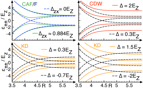
Figure 6: SP energy levels $\varepsilon_{\pm\pm}$ for the different phase regimes as they are obtained from the analytical formulas in Table 1. Upper left panel: CAF (solid, green lines), F (blue, dashed lines). Upper right panel: CDW for $|\Delta|>E_{Z}$ (solid, red lines) and $|\Delta|<E_{Z}$ (dashed, black lines). Lower left panel: KD for $|\Delta|<E_{Z}$ with $\Delta>0$ (solid, orange lines) or $\Delta<0$ (dashed, black lines). Lower right panel: KD for $|\Delta|>E_{Z}$ with $\Delta>0$ (solid, orange lines) or $\Delta<0$ (dashed, black lines). Depending on the sign and the magnitude of $\Delta$, the different cases for the SP spectra differ in the number of level crossings, even within one and the same phase.

We now diagonalize the single-particle HF Hamiltonian. The spectrum of the excited states is of particular interest, since the conduction properties of real graphene samples are governed by the edge modes in the QH regime. Recent conductance experiments have shown Young et al. (2014) that upon tilting the applied magnetic field there is a transition from an insulating regime to a phase where presumably edge states carry a nonzero current. Tilting the magnetic field corresponds to varying the parameter $u_{\perp}/E_{Z}$ in the system. The experimental observations therefore suggest that the gap to excited states in the edge spectrum varies as a function of $u_{\perp}/E_{Z}$ and closes, eventually, giving rise to a metal-insulator transition. We write the one-body HF Hamiltonian $\text{h}^{HF}$ corresponding to the full Hamiltonian $\mathcal{H}$ of Eq. (7). It consists of four terms :

$$\text{h}_{\mu\nu}^{HF}(p)=-E_{kin}(p)[\tau_{x}]_{\mu\nu}-E_{Z}[\sigma_{z}]_{\mu\nu}+\;^{C}\Delta_{\mu\nu}+\;^{A}\Delta_{\mu\nu},$$ (21)

which we obtain via standard HF decoupling. For the mean-field potential from the Coulomb interaction Hamiltonian of Eq. (10) we find

$${}^{C}\Delta_{\mu\nu}=-u_{0}[gg^{\dagger}]_{\mu\nu},$$ (22)

where $u_{0}$ describes the exchange term of the Coulomb interaction Hamiltonian of Eq. (10). This formula is valid provided we neglect the spatial dependence of $g$. It means that we do not capture the spin texture effects of the exchange. For completeness, in the following analytical calculations and expressions, the Coulomb contribution of Eq. (22) will be written explicitly. The mean-field potential due to the interactions breaking SU(4) symmetry is given by :

$${}^{A}\Delta_{\mu\nu}=\sum_{\alpha}u_{\alpha}\Big{(}[\tau_{\alpha}]_{\mu\nu}\,\text{Tr}[gg^{\dagger}\tau_{\alpha}]-[\tau_{\alpha}gg^{\dagger}\tau_{\alpha}]_{\mu\nu}\Big{)}.$$ (23)

Within HF mean-field theory, diagonalizing $\text{h}^{HF}$ provides access to SP energies $\varepsilon_{i}$, satisfying $\text{h}^{HF}|i\rangle=\varepsilon_{i}|i\rangle$, where the state labeled by $i$ stands for the $i$th SP HF eigenstate. In the following, we assume the eigenvalues to be ordered $\varepsilon_{1}\leq\varepsilon_{2}\leq\varepsilon_{3}\leq\varepsilon_{4}$. In earlier work Kharitonov (2012b), this Hamiltonian has been studied with the assumption of constant order parameter to the edge.

However, the explicit effective valley field due to the edge certainly invalidates this simple assumption. It should be noted also that in the intermediate regime between the bulk state and the edge regime the HF ground state is no longer a simple tensor product state even within the HF approximation and there is some nontrivial spin/valley entanglement. To facilitate subsequent discussion we summarize the results of Ref. Kharitonov, 2012b in Table 1. The analytical expressions for the mean-field levels were presented in Ref. Kharitonov, 2012b for the F/CAF cases. A straightforward calculation allows direct extension to the KD and the CDW configuration. Examples for the SP energy levels $\varepsilon_{\pm\pm}$ obtained within this approximation for the different phases are plotted in Fig. 6 for various choices of the couplings.

CAF/F phase:

${}^{A}\Delta=\;^{A}\Delta_{0z}\mathbb{1}\otimes\sigma_{z}+\;^{A}\Delta_{zx}\sigma_{z}\otimes\sigma_{x}$

with ${}^{A}\Delta_{0z}=-\frac{1}{2}(u_{0}+u_{z}+2u_{\perp})\cos{\theta}$ and ${}^{A}\Delta_{zx}=-\frac{1}{2}(u_{0}+u_{z}-2u_{\perp})\sin{\theta}$,

$\varepsilon_{\pm\pm}=\pm\sqrt{\big{[}E_{kin}(p)\pm\big{(}E_{Z}-\;^{A}\Delta_{0z}\big{)}\,\big{]}^{2}+\big{(}\,^{A}\Delta_{zx}\big{)}^{2}}$,

$\Delta\varepsilon_{edge}=2\;|\,^{A}\Delta_{zx}|,$ $\Delta\varepsilon^{CAF}_{bulk}=u_{0}+u_{z}-2u_{\perp},$ $\Delta\varepsilon^{F}_{bulk}=2|E_{Z}-\,^{A}\Delta_{0z}|$.

CDW/KD phase:

${}^{A}\Delta=\;^{A}\Delta_{x0}\sigma_{x}\otimes\mathbb{1}+\;^{A}\Delta_{y0}\sigma_{y}\otimes\mathbb{1}+\;^{A}\Delta_{z0}\sigma_{z}\otimes\mathbb{1}$

with ${}^{A}\Delta_{x,y0}=-\frac{1}{2}(u_{0}t_{x,y}-u_{z}t_{x,y}-4u_{\perp}t_{x,y})$ and ${}^{A}\Delta_{z0}=-\frac{1}{2}(u_{0}t_{z}-3u_{z}t_{z}-2u_{\perp}t_{z})$,

which implies ${}^{A}\Delta^{CDW}_{z0}=-\frac{1}{2}(u_{0}-3u_{z}-2u_{\perp})$ and ${}^{A}\Delta^{KD}_{x0}=-\frac{1}{2}(u_{0}-u_{z}-4u_{\perp})$,

$\varepsilon^{CDW}_{\pm\pm}=\pm E_{Z}\pm\sqrt{E_{kin}(p)\,^{2}+\big{(}\,^{A}\Delta^{CDW}_{z0}\big{)}^{2}},$ and $\varepsilon^{KD}_{\pm\pm}=\pm E_{Z}\pm[E_{kin}(p)-\,^{A}\Delta^{KD}_{x0}]$,

$\Delta\varepsilon_{bulk}=2|E_{Z}-|^{A}\Delta_{z0/x0}||.$

Table 1: Analytical expressions for the mean-field potential of the symmetry-breaking terms, ${}^{A}\,\Delta$, the eigenvalues of the full mean-field Hamiltonian, $\varepsilon_{\pm\pm}$, and the minimum gaps in the bulk and at the edge, $\Delta\varepsilon_{bulk/edge}$. We denote by $\mathbf{s}$ and $\mathbf{t}$ the SP spin and isospin configuration of the two electrons per orbital and $\theta$ describes the canting angle between the two spins. In all the formulas for the mean-field potentials, we dropped a constant term $-\frac{1}{2}(u_{0}+2u_{\perp}+u_{z})\mathbb{1}\otimes\mathbb{1}$. These analytical results have been obtained within the approximation that the bulk phase does not change as a function of space when approaching the edge.

The ansatz that we introduced in Secs. II and III is able to describe spatial dependence of the order and also to capture spin/valley entanglement.

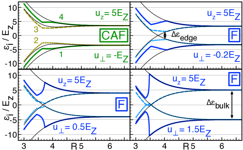
Figure 7: Spatial behavior of the energetic SP spectra in the presence of a boundary for positive transverse coupling $u_{z}=5E_{Z}$ and different values of the perpendicular coupling $u_{\perp}$ : CAF bulk phase at $u_{\perp}=-E_{Z}$ in the upper left panel (green lines), F bulk phase at $u_{\perp}=-0.2E_{Z}$, $u_{\perp}=0.5E_{Z}$, and $u_{\perp}=1.5E_{Z}$ in the remaining panels, respectively (blue lines). Thick, colorful lines show our numerical results. Here, different line shapes distinguish between the different single-particle energy levels $\varepsilon_{1}\leq\varepsilon_{2}\leq\varepsilon_{3}\leq\varepsilon_{4}$. Thin, black lines compare to the analytical formulas for $\varepsilon_{\pm\pm}(R)$ listed in Table 1 for the different phases, respectively, in which no modulation of the underlying spin/isospin texture towards the edge is taken into account. We see two bulk levels, being two-fold degenerate and separated by a gap of width $\Delta\varepsilon_{bulk}$ in the bulk, split into four branches when approaching the edge. The branches exhibit kinks and regimes of different behavior corresponding to the transitions between different spin and isospin phases during the evolution from the bulk to the edge (see Fig. 3). The edge gap between the two intermediate levels $\varepsilon_{2}$ and $\varepsilon_{3}$ (dotted and dashed lines, respectively) $\Delta\varepsilon_{edge}=\text{min}(|\varepsilon_{3}-\varepsilon_{2}|]$ remains finite over a certain range of $u_{\perp}$, reducing gradually as $u_{\perp}$ increases until it finally closes completely. The lower right panel shows a configuration were the levels cross and form gapless edge states. Special attention should be paid to the upper right panel and the lower left panel in which the numerical results show configurations with a F phase in the bulk were finite edge gaps $\Delta\varepsilon_{edge}\neq 0$ remain, whereas the analytical curves cross as soon as the bulk passes into an F phase. The behavior of the $\Delta\varepsilon_{edge}$ as a function of $u_{\perp}$ is studied further in Fig. 9.

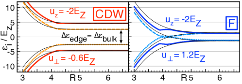
Figure 8: Same as Fig. 7 for $u_{z}=-2E_{Z}$ and different $u_{\perp}$, hence displaying the SP spectra for the bulk phase regimes of the lower half plane of the GS phase diagram. Left panel: CDW bulk phase at $u_{\perp}=-0.6E_{Z}$ (red lines). Right panel: F bulk phase at $u_{\perp}=-1.3E_{Z}$ (blue lines). Thin, black lines compare to the analytical formulas given in Table 1 for the different phases, respectively, in which the evolution of the bulk’s phase towards the edge is neglected. For the CDW wave phase in the left panel we observe four non-degenerate SP levels in the bulk; furthermore, as these levels do not bend towards each other but disperse when approaching the edge, the minimum energy gap to SP excitations is given by the bulk gap $\Delta\varepsilon_{edge}=\Delta\varepsilon_{bulk}$.

We obtain the set of parameters $\{\alpha(R),\beta(R),\chi(R)\}$ characterizing the GS $|g\rangle$, by minimizing the total energy $E_{tot}$ of Eq. (15). From these space-dependent parameters, we construct the corresponding density matrix $\rho_{g}=gg^{\dagger}$ via Eq. (18), which in turn allows us to reconstruct and diagonalize $\text{h}^{HF}$ of Eq. (21). The analysis is repeated for every point in space, thereby yielding the spatial behavior as a function of the distance from the edge. The results for the spectra $\varepsilon_{i}$ established near the edge for different phases in the bulk are shown in Figs. 7 and 8. We have chosen the same parameters as in the plots of Figs. 3 and 5. For $u_{z}>0$ in Fig. 7, we explore the upper half plane, whereas for $u_{z}<0$ (Fig. 8), the evolution of the bulk phases of the lower half-plane is displayed. In all figures the thick colorful lines show the outcome of our numerical studies. The thin black lines represent the analytical results for the SP energy levels for the phase established in the bulk at the particular system parameters shown, as given in Table 1. Figure 7 illustrates the evolution of the edge SP levels for a transverse coupling energy of $u_{z}=5E_{Z}$ and different values of the perpendicular coupling $u_{\perp}$, for which the bulk phase configuration passes from a CAF phase at $u_{\perp}=-E_{Z}$ (green lines, upper left panel) to a F phase at $u_{\perp}=-0.2E_{Z},u_{\perp}=0.5E_{Z}$, and $u_{\perp}=1.5E_{Z}$, respectively (blue spectra in the upper right and the two lower panels). In general, the spectra in all four panels show the following behavior : two flat energy levels, separated by the gap $\Delta\varepsilon_{bulk}$, are present in the bulk, both two-fold degenerate and they split into four branches when approaching the edge. The two intermediate levels, being labeled $\varepsilon_{2}$ and $\varepsilon_{3}$, first bend towards each other, establishing the minimum energy gap $\Delta\varepsilon_{edge}<\Delta\varepsilon_{bulk}$, before, even closer to the edge, the two lowest and the two highest levels $\varepsilon_{1},\varepsilon_{2}$ and $\varepsilon_{3},\varepsilon_{4}$ are driven apart in two parallel pairs, respectively.

In Fig. 8, we show the spectra corresponding to the phases of the lower half plane : at $u_{z}=-2$, we display the energy levels at $u_{\perp}=-0.6E_{Z}$ (red lines in the left panel), for which the bulk is CDW as well as for $u_{\perp}=1.2E_{Z}$ (blue lines in the right panel), where the bulk is F. The behavior of the SP energy levels in a CDW bulk phase qualitatively differs from the situation of the CAF/F phase described above. In the left panel of Fig. 8 there are four non-degenerate levels in the bulk. In contrast to the levels of the CAF/F case, they do not bend towards each other and there is no minimum energy induced by the edge behavior. Hence, we find that the minimum edge gap is equal to the bulk gap : $\Delta\varepsilon_{edge}=\Delta\varepsilon_{bulk}$. Sufficiently close to the edge, the levels again form two parallel pairs. The spectra for the KD phase in the bulk are not shown because, as mentioned in Sec. IV, this state does not undergo any significant evolution when approaching the edge. The spectra do not differ from the analytical prediction for $\varepsilon_{\pm\pm}$ shown for ${}^{A}\Delta_{x0}^{KD}$ in the lower right panel of Fig. 6.

When comparing this behavior to the analytical results as given in Table 1 (black lines), deep in the bulk we find that all curves coincide as they should. Furthermore, from the discussion in Sec. IV.2, we know that there is no spin-valley entanglement in the bulk, i.e., the bulk states indeed are of separable product form. Yet, significant deviations between the numerical results capturing the full GS properties and the analytical curves from the simplified treatment are observed when moving closer to the edges, where the GS spin/isospin configuration starts to deviate from the bulk phase; cf. Fig. 3. The SP energies $\varepsilon_{i}$ have kinks whenever the underlying spin/isospin texture changes and exhibit qualitatively different behavior in the different texture regimes. Thus, the emergence of different spin/isospin configurations due to the edge potential when approaching the edges directly translates into the SP spectra leading to a complex energy structure as a function of space.

V.2 Single Particle Level Crossings in the different Texture Regimes

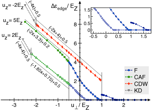
Figure 9: Behavior of the gap $\Delta\varepsilon_{edge}$ in the SP spectra close to the edge. We use three couplings : $u_{z}=-2E_{Z}$, $u_{z}=2E_{Z}$, and $u_{z}=5E_{Z}$ (filled, shaded and empty symbols, respectively). Different colors and symbols stand for different bulk phases: KD (grey triangles), CDW (red diamonds), CAF (green squares), and F phase (blue circles). Dashed, colored lines connect the data points as a guide to the eye. The dotted, black lines represent the behavior of the data in the linear regimes (they are shifted by a constant offset with respect to the curves for better visibility). Gray vertical lines indicate the critical values for bulk phase transitions. For all phases the gap $\Delta\varepsilon_{edge}$ monotonically decreases as $u_{\perp}$ grows until it finally closes in the regime where the bulk is in an F phase. The inset is a close-up on how the blue lines smoothly approach $\Delta\varepsilon=0$. The transitions from $\Delta\varepsilon_{edge}\neq 0$ to $\Delta\varepsilon_{edge}=0$ take place at $u_{\perp}\approx\,0.3E_{Z}$, $u_{\perp}\approx\,E_{Z}$, $u_{\perp}\approx\,1.625E_{Z}$.

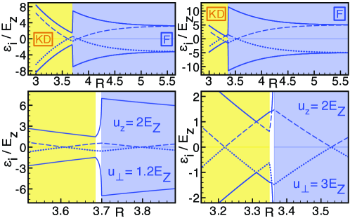
Figure 10: Close-up on the SP spectra in the regime with multiple crossings for $u_{z}=2E_{Z}$. Left side: $u_{\perp}=1.2E_{Z}$, right side: $u_{\perp}=3E_{Z}$. The blue lines show the SP energy levels $\varepsilon_{i}$. The different background colors mark the spatial regimes in which the GS establishes different spin/isospin textures: there is a F phase (blue region). In the intermediate (white) region, the system undergoes a transition before it finally ends up in a KD phase (yellow region). We observe the crossings of the SP levels to occur in regions of different spin/isospin phases - their origins lie in the different symmetries of the F and KD phases.

The energy levels of the SP ground and excited states show a complex structure as a function of space depending on the spatial changes of the spin and isospin texture when approaching the graphene edge. In particular, in some configurations, the SP spectra exhibit a finite gap, whereas for other system parameters, the edge states are gapless when the SP levels cross. In this section, we investigate the crossings between SP energy levels which leads to gapless edge excitations. We first discuss the properties of the edge gap and its behavior when approaching the critical values where it closes. Then, we explain the number of allowed crossing points between energy levels and the connection to the symmetry properties of the underlying spin/isospin texture phases. The spatial variation of the order parameters has a direct impact on the overall shape of the dispersion of edge modes. This is readily seen in Figs. 7 and 8, where we plot the dispersions from our calculation including edge effects and results from a similar calculation using only bulk values without spatial variation. In order to investigate the closure of the edge gap $\Delta\varepsilon_{edge}$ as a function of the ratio $u_{\perp}/E_{Z}$, we evaluate the size of the minimum gap in the SP spectra for various system parameters. We choose the same values for the anisotropy energies as in Sec. IV by fixing $u_{z}=5E_{Z},u_{z}=2E_{Z}$ and $u_{z}=-2E_{Z}$ and varying $u_{\perp}$ so that we access all bulk phases in the GS phase diagram. The resulting curves $\Delta\varepsilon_{edge}({u_{\perp}}/{E_{Z}})$ are shown in Fig. 9. We find that the size of the edge gap $\Delta\varepsilon_{edge}$ is a strictly monotonic decreasing function of ${u_{\perp}}/{E_{Z}}$ for all values of $u_{z}$. When the bulk is KD or CDW the flat bulk SP levels split further apart when approaching the edge so that the minimum gap in the spectrum is equal to the bulk gap $\Delta\varepsilon_{edge}=\Delta\varepsilon_{bulk}$. In these two cases we find that the bulk gap is a linear function of the perpendicular coupling energy : $\Delta\varepsilon_{bulk}^{KD/CDW}\propto u_{\perp}/E_{Z}$. The numerical results in Fig. 9 follow exactly the analytical prediction given in Table 1 : At $u_{z}=-2E_{Z}$, we find $\Delta\varepsilon^{KD}_{bulk}=-4u_{\perp}$ and $\Delta\varepsilon^{CDW}_{bulk}=-2u_{\perp}+4E_{Z}$, whereas the KD edge gap at $u_{z}=2E_{Z}$ behaves as $\Delta\varepsilon^{KD}_{bulk}=-4u_{\perp}-4E_{Z}$. These analytical curves are plotted in Fig. 9 as dotted lines for comparison (they are shifted by a constant offset with respect to the numerical results for better visibility). As a consequence of this linear behavior in $u_{\perp}$, for couplings favoring KD or CDW in the bulk, at the system parameters chosen in Fig. 9, there is always a non-zero gap to SP excitations. When the GS in the bulk is a CAF or a F phase, the SP spectra now bend towards each other and therefore exhibit a minimum energy gap $\Delta\varepsilon_{edge}$ near the edge which is smaller than the bulk gap.

For $u_{\perp}\leq-E_{Z}/2$ where the bulk is a CAF phase (green squares), the spectrum always exhibits an non-zero edge gap which is almost linear as a function of the perpendicular coupling. At values $u_{\perp}\geq-E_{Z}/2$, hence for a F bulk, the shape of the spectrum changes qualitatively and the bulk gap closes in a non-linear way, asymptotically approaching zero at sufficiently large values of $u_{\perp}$. For the transverse couplings chosen in Fig. 9, $u_{z}=5\,E_{Z}$, $u_{z}=2\,E_{Z}$, and $u_{z}=-2\,E_{Z}$, the edge gap $\Delta\varepsilon_{edge}$ closes at $u_{\perp}\approx\,E_{Z}$, $u_{\perp}\approx\,0.3E_{Z}$, and $u_{\perp}\approx\,1.6E_{Z}$, respectively. All these values leads to a bulk which is ferromagnetic. So the prediction for the gap closure point clearly differs from the value $u_{\perp}=-\frac{E_{Z}}{2}$, which can be read from the bulk phase diagram in Fig. 2. This is due to the changes of the spin/isospin configuration of the GS induced by the effective edge potential as we approach the boundary; cf. Fig. 3 of Sec. IV. Indeed the system does not remain in a F phase configuration all the way from the bulk to the edge. During its transition into a KD phase close to the boundary, there is an intermediate regime with non-zero spin-valley entanglement and simultaneous canting of both spin and isospin. Hence, in this transition regime there is no a priori justification for $\Delta_{edge}^{CAF/F}$ of Table 1 to yield a correct description of the edge gap.

From this analysis of the gaps of the SP spectra we can draw the following conclusion : when the bulk is CDW, KD or CAF phase, the SP energy levels always have non-zero gaps. However for a bulk F phase one may have gapped or gapless spectra. We note that ignoring the spatial variation of the trial HF state leads to qualitatively different results Kharitonov (2012b).

V.3 Number of level crossings

We now discuss in more detail the number of crossings of the HF single-particle states. In the F phase with dispersion $\varepsilon_{\pm\pm}^{F}$ in Table 1, the intersecting levels $\varepsilon_{+-}^{F}$ and $\varepsilon_{--}^{F}$ cross exactly once as their slope is given by the slope of the kinetic energy term and they are monotonic functions of the spatial coordinate. For several system parameters, such as in the spectrum in the lower left panel of Fig. 7 at $u_{z}=5E_{Z},u_{\perp}=1.5E_{Z}$ as well as in close ups shown in Fig. 10, we observe multiple crossings. We first discuss the occurrence of multiple crossings and the relation with the underlying spin/valley texture. The number of crossings is governed by the symmetries of the HF Hamiltonian and the magnitude of the HF self-consistent potentials. After discussing the different phases separately, we apply the insights to the edge state structure described in Sec. IV, where the GS phase changes as a function of space when approaching the edge from the bulk. We first discuss the case of the CAF/F transition. We rewrite the mean-field Hamiltonian of Eq. (21) involving the CAF/F mean-field potential given in Table 1 by decomposing it into four $2\times 2$ matrices as :

$$\text{h}^{HF}(p)=\begin{bmatrix}\gamma_{1}&\gamma_{2}\\ \gamma_{3}&\gamma_{4}\end{bmatrix},$$ (24)

where the respective entries for the CAF/F phase are given by :

$$\gamma_{1} =\,^{A}\Delta_{zx}\sigma_{x}-(E_{Z}-\,^{A}\Delta_{0z})\,\sigma_{z},$$

$$\gamma_{2} =\gamma_{3}=-E_{kin}(p)\;\mathbb{1},$$

$$\gamma_{3} =-\,^{A}\Delta_{zx}\,\sigma_{x}-(E_{Z}-\,^{A}\Delta_{0z})\,\sigma_{z},$$ (25)

with $\,{}^{A}\Delta_{zx}$ and $\,{}^{A}\Delta_{0z}$ defined for the CAF/F phase in Table 1. The size of the gap is therefore governed by the first off-diagonal coupling matrix elements $\,{}^{A}\Delta^{CAF/F}_{zx}$. If $\,{}^{A}\Delta^{CAF/F}_{zx}\neq 0$, as is the case for any non-zero canting angle $\theta\neq 0$, the eigenvalues of the Hamiltonian $\text{h}^{HF}_{CAF/F}$ exhibit the characteristic behavior of avoided crossings. The SP levels are allowed to cross only for $\,{}^{A}\Delta^{CAF/F}_{zx}=0$ at $\theta=0$, i.e., in the F phase. In the bulk, i.e., at $E_{kin}\equiv 0$, all values of the coupling energies $u_{z}$ and $u_{\perp}$ allowed for the F phase yield the same ordering of the SP energy levels $\varepsilon_{\pm\pm}^{F,0}=\varepsilon_{\pm\pm}^{F,0}(E_{kin}\equiv 0)$, independently of the sign or the modulus of $\Delta_{0z}^{CAF/F}$: $\varepsilon_{+-}^{F,0}=\varepsilon_{-+}^{F,0}<0<\varepsilon_{--}^{F,0}=\varepsilon_{++}^{F,0}$. Hence, there is only one possible scenario of level crossings when approaching the boundary as the increasing edge potential is driving the SP levels away from their bulk values. This leads to exactly one crossing of the levels $\varepsilon_{+-}^{F}$ and $\varepsilon_{--}^{F}$, shown by the blue, dashed lines in the upper left panel of Fig. 6. We can perform the same analysis for CDW or KD phases. Again, we rewrite the corresponding HF Hamiltonians of Eq. (21) with the potentials $\,{}^{A}\Delta^{CDW/KD}_{z0/x0}$ from Table 1 and we find the respective entries for the CDW :

$$\gamma_{1} =-E_{Z}\,\sigma_{z}+\,^{A}\Delta_{z0}\,\mathbb{1},$$

$$\gamma_{2} =\gamma_{3}=-E_{kin}(p)\,\mathbb{1},$$

$$\gamma_{4} =-E_{Z}\,\sigma_{z}-\,^{A}\Delta_{z0}\,\mathbb{1},$$ (26)

whereas for the KD phase we find :

$$\gamma_{1} =\gamma_{4}=E_{Z}\,\sigma_{z},$$

$$\gamma_{2} =\gamma_{3}=\Big{(}\,^{A}\Delta^{KD}_{x0}-E_{kin}(p)\Big{)}\,\mathbb{1}.$$ (27)

The Hamiltonians for the CDW phase and the KD phase thus turn out to have higher symmetry than in the CAF phase: In $\text{h}^{HF}_{CDW}$ and $\text{h}^{HF}_{KD}$, all entries of the two first off-diagonals as well as of the antidiagonal are zero. Pairwise degeneracy of the corresponding eigenvalues, i.e., crossings between the SP energy levels, is now allowed. Note that, unlike the transition from a CAF to a F phase, all other transitions do not correspond to smooth transitions. In these cases, a transition between phases goes along with an abrupt change of the symmetry properties of the spin/isospin configuration of the GS and the corresponding Hamiltonian.

We now discuss the different possible scenarios of SP level crossings in CDW and KD phases. The SP energy levels of the CDW $\varepsilon_{\pm\pm}^{CDW}$ in Table 1 are independent of the sign of $\,{}^{A}\Delta^{CDW}_{z0}$. Different orderings of the bulk levels $\varepsilon_{\pm\pm}^{CDW,0}$ at $E_{kin}\equiv 0$ may, however, appear depending on the modulus of $\,{}^{A}\Delta^{CDW}_{z0}$ : for $|\,^{A}\Delta^{CDW}_{z0}|>E_{Z}$, the bulk states are ordered as $\varepsilon_{--}^{CDW,0}<\varepsilon_{+-}^{CDW,0}<\varepsilon_{-+}^{CDW,0}<\varepsilon_{++}^{CDW,0}$. In this case, when approaching the boundary, the kinetic energy potential drives the positive and the negative energy states further apart from each other such that they do not cross. In the case where $|\,^{A}\Delta^{CDW}_{z0}|<E_{Z}$, however, the bulk states rather follow the hierarchy $\varepsilon_{--}^{CDW,0}<\varepsilon_{-+}^{CDW,0}<0<\varepsilon_{+-}^{CDW,0}<\varepsilon_{++}^{CDW,0}$. In this case, turning on the effective edge potential drives the levels $\varepsilon_{-+}^{CDW,0}$ and $\varepsilon_{+-}^{CDW,0}$ towards each other and they cross at zero energy. These two different scenarios are depicted in the upper right panel of Fig. 6, where the red, solid lines show the levels $\varepsilon_{\pm\pm}^{CDW}$ from Table 1 at $\,{}^{A}\Delta^{CDW}_{z0}=2E_{Z}>E_{Z}$ and the black, dashed lines show the spectrum for $\,{}^{A}\Delta^{CDW}_{z0}=0.3E_{Z}<E_{Z}$. The latter case, $|\,^{A}\Delta^{CDW}_{z0}|<E_{Z}$, however, is prohibited by the conditions imposed on the couplings $u_{z}$ and $u_{\perp}$ in order for the system to establish a CDW phase in the bulk. Requiring $u_{z}<u_{\perp}$ and $u_{z}<-E_{Z}-u_{\perp}$ will always force $|\,^{A}\Delta^{CDW}_{z0}|>E_{Z}$. Therefore, treating the system as having a stable CDW phase in the bulk and all the way to the edge will never lead to any crossings of the SP edge levels. Turning to the more important case of the KD phase, the situation becomes even richer. Here, depending on the sign and the modulus of ${}^{A}\Delta^{KD}_{x0}$, four different SP level orderings in the bulk and four resulting crossing scenarios may appear. For $|^{A}\Delta^{KD}_{x0}|<E_{Z}$, if ${}^{A}\Delta^{KD}_{x0}>0$, there is one level crossing at zero energy and two additional crossings above and below the zero energy line, respectively, whereas for negative ${}^{A}\Delta^{KD}_{x0}$, only one crossing at zero energy is present. The case $|^{A}\Delta^{KD}_{x0}|>E_{Z}$ can lead to four crossings, two at zero energy plus one above and one below, respectively, if $\Delta^{KD}_{x0}>0$, whereas for ${}^{A}\Delta^{KD}_{x0}<0$, the four levels do not cross.

Examples of the four different cases are shown in the lower panels of Fig. 6, where the lower left panel shows the possible situations for $|\,^{A}\Delta^{KD}_{x0}|<E_{Z}$ (solid, orange lines for $\,{}^{A}\Delta^{KD}_{x0}=-0.3E_{Z}<0$ and black dashed lines for $\,{}^{A}\Delta^{KD}_{x0}=0.7E_{Z}>0$), whereas the right panel displays the corresponding spectra for $|\,^{A}\Delta^{KD}_{x0}|>E_{Z}$ (here, the solid, orange lines are for $\,{}^{A}\Delta^{KD}_{x0}=-1.5E_{Z}<0$ and black dashed lines for $\,{}^{A}\Delta^{KD}_{x0}=2E_{Z}>0$). Note that, just as in the case of the CDW phase, not all these cases are allowed by the restrictions on the parameter range for a KD bulk : requiring the couplings $u_{z}$ and $u_{\perp}$ to fulfill the relations $u_{\perp}<u_{z}$ and $u_{z}<\frac{E_{Z}^{2}}{2u_{\perp}}-u_{\perp}$ always implies $\,{}^{A}\Delta^{KD}_{x0}>E_{Z}$. Therefore, again, all cases including possible crossings between edge levels are ruled out for a system with a KD phase in the bulk.

This simple picture drawn for constant order parameters changes when considering the electronic GS structure described in Sec. IV. Indeed the GS spin/isospin texture deviates from the bulk phase when moving towards the edge as a consequence of the growing edge potential. Close enough to the edge the system is always driven into a KD phase. Hence when moving sufficiently close to the edge the GS does becomes KD-ordered, even though the system parameters $u_{z}$ and $u_{\perp}$ do not allow KD order in the bulk. Two examples are shown in the close-ups in Fig. 10. Parameters in both panels are chosen such that the bulk system at $E_{kin}\equiv 0$ is in a F phase. When moving towards the edge the energy levels evolve according to $\varepsilon_{\pm\pm}^{F}$ of Table 1 (corresponding to the evolution within the blue region). A first crossing between the intermediate levels occurs, as predicted by the analysis of the F phase energy levels. After the transition region (left white), the GS becomes KD (marked by the yellow shading). However, the system parameters do not force $\,{}^{A}\Delta^{KD}_{x0}>E_{Z}$ : in the left panel of Fig. 10, we find $\,{}^{A}\Delta^{KD}_{x0}=-3.4E_{Z}$ and in the right panel we have $\,{}^{A}\Delta^{KD}_{x0}=-7E_{Z}$. Therefore the energy levels now evolve according to $\varepsilon_{\pm\pm}^{KD}$ of Table 1 in the case ${}^{A}\Delta^{KD}_{x0}<0,\;|\,^{A}\Delta^{KD}_{x0}|<E_{Z}$. As a consequence, in this regime, one more level crossing may occur. Hence, the appearance of several crossings of the SP energy levels in the numerical spectra as in the lower right panel of Fig. 7 and in Fig. 10 can be explained combining the insight of Sec. IV that any bulk phase by the edge potential always is driven into a KD phase close to the boundary, with the understanding of the possible behavior of $\varepsilon_{\pm\pm}^{KD}$ depending on the value of $\,{}^{A}\Delta^{KD}_{x0}$ as a function o the coupling energies $u_{z}$ and $u_{\perp}$. The SP energy levels describing the numerical results of Figs. 7, 8, and 10 can be summarized as :

$$\varepsilon_{\pm\pm}(R)=\begin{cases}\varepsilon_{\pm\pm}^{bulk}(R)&\text{for }R>R_{2},\\ \text{unknown }&\text{for }R_{1}<R<R_{2},\\ \varepsilon_{\pm\pm}^{KD}(R)&\text{for }R<R_{1},\end{cases}$$ (28)

where $\varepsilon_{\pm\pm}^{bulk}(R)$ denotes the level spectra for the bulk phase established at a given choice of system parameters and $R_{2}$ and $R_{1}$ label the inner and outer limits in space of the domain wall, for which there is no simple analytic expression. The evolution of $\varepsilon_{\pm\pm}^{KD}(R)$ is no longer limited to the non-crossing behavior imposed for a bulk KD phase but it can exhibit any of the shapes drawn in the two lower panels of Fig. 6. Which of these curves describes the KD-like evolution of the edge states correctly is determined by the system parameters $u_{\perp}$ and $u_{z}$ that govern the bulk texture phase. From the analysis of the number of SP level crossings we hence learn that, in principle, by choosing appropriate values of $u_{z}$ and $u_{\perp}$, SP energy levels can have zero, one, two, or even three crossings at zero energy. Among these crossings, one is due to the symmetry properties of the bulk F phase. The remaining crossings appear in the KD phase close to the boundary, which in this regime shows novel properties not present for a KD phase in the bulk. We note that these crossings occur at different distances from the edge - at the distance where the corresponding KD phase SP levels for a certain $\,{}^{A}\Delta^{KD}_{x0}$ cross, it is necessary for the system already to have evolved from the bulk phase into the KD edge phase in order for the additional SP level crossings to occur. This is the reason why we do not see any crossings in the SP spectrum shown in the lower left panel of Fig. 8 where the bulk is in a CDW phase : at the distance $R_{cross}$ where the KD-like levels near the edge would cross, the system still behaves according to its bulk CDW phase. In this case, the crossing is thus prevented by the fact that the crossing point lies outside the KD region : $R_{cross}>R_{2}$. Nevertheless, a situation in which the bulk is a CDW but the SP edge states are gapless due to crossings of the KD-like levels close to the boundary is not forbidden by the underlying symmetry principles as the restrictions for the coupling energies of the CDW bulk phase allow negative values of ${}^{A}\Delta_{x0}^{KD}$. The exact distances from the edge $R_{1},R_{2}$, or $R_{cross}$ which define the points of crossing, involve the explicit form of the kinetic energy $E_{kin}(R)$ as they are determined by the eventual dominance of the kinetic energy. Numerical values for $R_{1},R_{2}$, or $R_{cross}$ therefore strongly depend on the model potential chosen for $E_{kin}(R)$. This is not true, however, for the answer to the question of whether crossings are allowed or not since the values of ${}^{A}\Delta$ are determined generically by the system parameters $u_{\perp}$ and $u_{z}$.

V.4 Properties of the underlying SP States

In order to obtain a better understanding of the nature of the excited states we analyze the properties of the single-electron states. We compute the spin and isospin components $s_{z}(i)=\frac{1}{2}\langle i|\sigma_{z}|i\rangle$ and $t_{x}(i)=\frac{1}{2}\langle i|\tau_{x}|i\rangle$ and display the results as a function of space in Fig. 11.

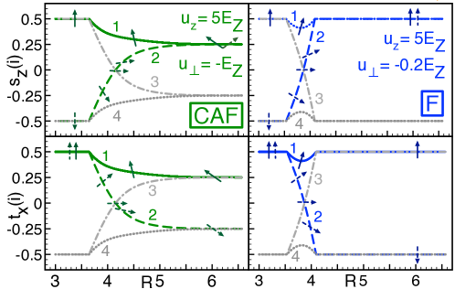
Figure 11: Evolution of the single-electron spin and isospin components $s_{z}(i)$ and $t_{x}(i)$ of the SP eigenstates from the bulk towards the edge for the two anisotropy energies $u_{\perp}=-E_{Z}$ (CAF bulk GS , left panels with green lines) and $u_{\perp}=-0.2\,E_{Z}$ (F bulk GS, right panels with blue lines). Different line shapes distinguish between the four SP energy levels $\varepsilon_{1}\leq\varepsilon_{2}\leq\varepsilon_{3}\leq\varepsilon_{4}$. Green/blue lines correspond to the observables of the two lowest-lying states which are occupied orbitals in the HF GS. Gray lines indicate the behavior of the higher-lying SP states. Arrows show the behavior of the spin and isospin polarizations. The second and third levels $|2\rangle$ and $|3\rangle$ are oppositely polarized in spin and isospin at the edge. In all plots we set $u_{z}=5\,E_{Z}$.

The evolution of the observables can be summarized as follows :

$$\begin{array}[]{cccc|cccc}s_{z}(i)&\text{edge}&\text{intermediate}&\text{bulk}\hskip 10.0pt&t_{x}(i)&\hskip 5.0pt\text{edge}&\text{intermediate}&\text{bulk}\\ \hline\cr s_{z}(1):&\uparrow&\nearrow&\uparrow&t_{x}(1):&\uparrow&\nearrow&\uparrow\\ s_{z}(2):&\downarrow&\searrow\longrightarrow\nearrow&\uparrow&t_{x}(2):&\uparrow&\nearrow\longrightarrow\searrow&\downarrow\\ s_{z}(3):&\uparrow&\nearrow\longrightarrow\searrow&\downarrow&t_{x}(3):&\downarrow&\searrow\longrightarrow\nearrow&\uparrow\\ s_{z}(4):&\downarrow&\swarrow&\downarrow&t_{x}(4):&\downarrow&\swarrow&\downarrow\end{array}$$ (29)

where arrows represent schematically the spin and isospin vectors.

The HF GS $|G\rangle$ is built from Slater determinants of $|1\rangle$ and $|2\rangle$ as the eigenstates of the two lowest lying branches $\varepsilon_{1}$ and $\varepsilon_{2}$ in Fig. 7. The lowest energy excitations correspond to single-particle excitation from the second to the third level $\varepsilon_{2}\rightarrow\varepsilon_{3}$. These two states have oppositely polarized spin and isospin components. The closing of the gap $\Delta\varepsilon_{edge}$ between the second and the third SP level in Fig. 11 hence is a transition from insulating to conducting behavior with the counterpropagating current-carrying edge states exhibiting opposite spin and isospin polarizations. This is the behavior of gapless helical edge states of a QSH state Hasan and Kane (2010).

VI Conclusion

The SU(4) QH ferromagnetism leads to a highly degenerate manifold of ground states for neutral graphene. This degeneracy is lifted by small lattice-scale anisotropies and there is a competition between phases with several types of order. This competition is affected notably by the substrate supporting the graphene sample. We have used a simple model of these anisotropies to study the edge properties of neutral graphene by means of a HF approach. The sharp atomic edge is then described by an effective field in valley space which modifies the competition between phases. Ultimately, whatever the bulk order, the system is in a KD phase close enough to the edge. In the transition region between this edge order and the bulk order, we have obtained evidence for an intermediate regime with spin/valley entanglement. In this regime there is a nontrivial change of the single-particle spectrum. We find that the number of levels crossing the Fermi energy can be varied by changing the parameter $u_{\perp}/E_{Z}$. This means that there are metal-insulator transitions when tilting the magnetic field. This is consistent with the experimental findings of Young et al. Young et al. (2014). If we adopt the estimates for the approximate magnetic field dependencies of $E_{Z}$ and $u_{\perp}$ stated in Refs. Kharitonov, 2012a and Kharitonov, 2012b as $E_{Z}(B)\approx 0.7$B [T]K and $u_{\perp}(B_{\perp})\approx 1-10B_{\perp}$[T]K, where $B$ denotes the total magnetic field and $B_{\perp}$ its component perpendicular to the device plane, the values for the parameters stated in Ref. Young et al., 2014 suggest that the authors were able to experimentally tune the ratio $u_{\perp}/E_{Z}$ roughly in a range from -13 to -0.5. The picture we obtain is more complex than that obtained by assuming that the order does not persist up to the edge Kharitonov (2012b). Notably the occurrence of the metal-insulator transition, while it sets constraints on the microscopic parameters, does not imply that the bulk is CAF ordered. The observation of a conductance $G\approx 2e^{2}/h$ which corresponds to two conducting channels, i.e., to one single level crossing, has two possible explanations : either the bulk is in a F phase leading to one crossing unaffected by the KD edge regime, or the bulk has noncrossing SP levels, but the crossing occurs in the KD regime close to the edge. Furthermore, our results suggest that the observation of exactly one crossing only corresponds to a limited parameter range. Varying the anisotropy parameters may lead to the observation of conductance values of higher multiples of two, corresponding to several crossings in the SP edge spectrum.

Of course there are obvious limitations of our theoretical approach : we apply a perturbative treatment of the edge, whose validity is limited to a certain range [cf. the discussion following Eq. (8)]. The appearance of a KD phase in the vicinity of the edge is a direct consequence of treating the effective edge potential perturbatively. Furthermore, in our calculations we assume the anisotropy energies $u_{\perp}$ and $u_{z}$ to remain constant at their bulk values [as we discuss after introducing Eq. (11)]. This approximation certainly becomes less exact as we approach the boundary. Also we have neglected the exchange energy effects that will create textures in the charge-carrying states.

In conclusion, in this paper we have studied the influence of an edge on the $\nu=0$ QH state in monolayer graphene. We found that the effective edge potential induces a change of the GS spin/isospin texture. During this evolution, novel phases are observed, involving simultaneous canting of spin and isospin as well as non-zero spin/valley entanglement. Phases of this kind are not present in the bulk. Furthermore, we analyzed how this spatial evolution changes the SP excited states. Here we have shown that, as a consequence of the spatial modulation of the underlying spin/isospin texture, the direct correspondence between the conductance properties of the edge states and the bulk phase is lost. The transport properties are governed by either zero, one, or multiple SP level crossings. The analysis of the SP eigenstates shows that the lowest SP excitation describes counterpropagating helical edge states carrying opposite spin and isospin polarizations.

- (1)
- (2) K. Nomura and A. H. MacDonald, Physical Review Letters 96, 256602 (2006).
- Yang et al. (2006) K. Yang, S. Das Sarma, and A. H. MacDonald, Physical Review B 74, 075423 (2006).
- (4) J. Alicea and M. P. A. Fisher, Physical Review B 74, 075422 (2006).
- (5) I. F. Herbut, Physical Review B 75, 165411 (2007).
- (6) I. F. Herbut, Physical Review B 76, 085432 (2007).
- Jung and MacDonald (2009) J. Jung and A. H. MacDonald, Physical Review B 80, 235417 (2009).
- Kharitonov (2012a) M. Kharitonov, Physical Review B 85, 155439 (2012a).
- Abanin et al. (2013) D. A. Abanin, B. E. Feldman, A. Yacoby, and B. I. Halperin, Physical Review B 88, 115407 (2013).
- Sodemann and MacDonald (2014) I. Sodemann and A. H. MacDonald, Physical Review Letters 112, 126804 (2014).
- Abanin et al. (2006) D. A. Abanin, P. A. Lee, and L. S. Levitov, Physical Review Letters 96, 176803 (2006).
- Chklovskii et al. (1992) D. B. Chklovskii, B. I. Shklovskii, and L. I. Glazman, Physical Review B 46, 4026 (1992).
- Chamon and Wen (1994) C. de C. Chamon and X. G. Wen, Physical Review B 49, 8227 (1994).
- Yang (2003) K. Yang, Physical Review Letters 91, 036802 (2003).
- Chang et al. (1996) A. M. Chang, L. N. Pfeiffer, and K. W. West, Physical Review Letters 77, 2538 (1996).
- Grayson et al. (1998) M. Grayson, D. C. Tsui, L. N. Pfeiffer, K. W. West, and A. M. Chang, Physical Review Letters 80, 1062 (1998).
- (17) Z.-X. Hu, R. N. Bhatt, X. Wan, and K. Yang, Physical Review Letters 107, 236806 (2011).
- Li et al. (2013) G. Li, A. Luican-Mayer, D. Abanin, L. Levitov, and E. Y. Andrei, Nature Communications 4, 1744 (2013).
- Fuhrer (2010) M. S. Fuhrer, Nature Materials 9, 611 (2010), ISSN 1476-1122.
- Cai et al. (2010) J. Cai, P. Ruffieux, R. Jaafar, M. Bieri, T. Braun, S. Blankenburg, M. Muoth, A. P. Seitsonen, M. Saleh, X. Feng, et al., Nature 466, 470 (2010), ISSN 0028-0836.
- Huang et al. (2012) H. Huang, D. Wei, J. Sun, S. L. Wong, Y. P. Feng, A. H. C. Neto, and A. T. S. Wee, Scientific Reports 2, 983 (2012), ISSN 2045-2322.
- (22) J. L. Lado and J. Fernández-Rossier, Physical Review B 90, 165429 (2014).
- Young et al. (2014) A. F. Young, J. D. Sanchez-Yamagishi, B. Hunt, S. H. Choi, K. Watanabe, T. Taniguchi, R. C. Ashoori, and P. Jarillo-Herrero, Nature 505, 528 (2014), ISSN 0028-0836.
- (24) B. Roy, M. P. Kennett, and S. Das Sarma, Physical Review B 90, 201409 (2014).
- (25) B. Roy, Physical Review B 89, 201401 (2014).
- (26) J. Alicea and M. P. A. Fisher, Solid State Communications 143, 504 (2007).
- (27) J.-N. Fuchs and P. Lederer, Physical Review Letters 98, 016803 (2007).
- (28) K. Nomura, S. Ryu, and D.-H. Lee, Physical Review Letters 103, 216801 (2009).
- (29) C.-Yu Hou, C. Chamon, and C. Mudry, Physical Review B 81, 075427 (2010).
- Kharitonov (2012b) M. Kharitonov, Physical Review B 86, 075450 (2012b).
- Brey and Fertig (2006a) L. Brey and H. A. Fertig, Physical Review B 73, 235411 (2006a).
- Brey and Fertig (2006b) L. Brey and H. A. Fertig, Physical Review B 73, 195408 (2006b).
- Fertig and Brey (2006) H. A. Fertig and L. Brey, Physical Review Letters 97, 116805 (2006).
- Murthy et al. (2014) G. Murthy, E. Shimshoni, and H. A. Fertig, Physical Review B 90, 241410 (2014).
- Castro Neto et al. (2009) A. H. Castro Neto, F. Guinea, N. M. R. Peres, K. S. Novoselov, and A. K. Geim, Reviews of Modern Physics 81, 109 (2009).
- Goerbig (2011) M. O. Goerbig, Reviews of Modern Physics 83, 1193 (2011).
- Akhmerov and Beenakker (2008) A. R. Akhmerov and C. W. J. Beenakker, Physical Review B 77, 085423 (2008).
- Mei and Lee (1983) W. N. Mei and Y. C. Lee, Journal of Physics A: Mathematical and General 16, 1623 (1983), ISSN 0305-4470.
- Janssen et al. (1994) M. Janssen, O. Viehweger, U. Fastenrath, and J. Hajdu, Introduction to the Theory of the Integer Quantum Hall Effect (Wiley-VCH, Weinheim ; New York, 1994), 427th ed., ISBN 9783527292097.
- Santos and Kaxiras (2013) E. J. G. Santos and E. Kaxiras, Nano Letters 13, 898 (2013), ISSN 1530-6984.
- Aleiner et al. (2007) I. L. Aleiner, D. E. Kharzeev, and A. M. Tsvelik, Physical Review B 76, 195415 (2007).
- (42) F. Wu, I. Sodemann, Y. Araki, A. H. MacDonald, and Th. Jolicoeur, Physical Review B 90, 235432 (2014).
- Kharitonov (2012c) M. Kharitonov, Physical Review Letters 109, 046803 (2012c).
- Ezawa et al. (2005) Z. F. Ezawa, M. Eliashvili, and G. Tsitsishvili, Physical Review B 71, 125318 (2005).
- Mintert et al. (2005) F. Mintert, A. R. R. Carvalho, M. Kuś, and A. Buchleitner, Physics Reports 415, 207 (2005), ISSN 0370-1573.
- Hasan and Kane (2010) M. Z. Hasan and C. L. Kane, Reviews of Modern Physics 82, 3045 (2010).