Communicability Angles Reveal Critical Edges for Network Consensus Dynamics

Abstract

We consider the question of determining how the topological structure influences a consensus dynamical processes taking place on a network. By considering a large dataset of real-world networks we first determine that the removal of edges according to their communicability angle—an angle between position vectors of the nodes in an Euclidean communicability space—increases the average time of consensus by a factor of $5.68$ in real-world networks. The edge betweenness centrality also identifies—in a smaller proportion—those critical edges for the consensus dynamics, i.e., its removal increases the time of consensus by a factor of $3.70$. We justify theoretically these findings on the basis of the role played by the algebraic connectivity and the isoperimetric number of networks on the dynamical process studied, and their connections with the properties mentioned before. Finally, we study the role played by global topological parameters of networks on the consensus dynamics. We determine that the network density and the average distance-sum—an analogous of the node degree for shortest-path distances, account for more than 80% of the variance of the average time of consensus in the real-world networks studied.

¹Department of Mathematics and Statistics, University of Strathclyde, 26 Richmond Street, Glasgow G1 1HX, United Kingdom

PACS number(s): 89.75.-k, 02.10.Ox, 05.45.Xt

1 Introduction

Complex networks are ubiquitous in many real-world systems ranging from biological and ecological to social and infrastructural ones [1]. One of the most important aspects of these networked systems is the transmission of information from one node to another. It can be argued indeed that networks exist for facilitating the information transmission in those complex systems. The nodes of these networks represent the entities of the complex system and their connections represent the interactions among these entities from which information flows from one node to another. Information is understood here generically and can represent such a variety of things like the transfer of material or energy to the spread of diseases or rumors.

The diffusion of information over a network is usually analyzed by considering that the state of the nodes of the graph at time $t$ are stored in a vector $\vec{u}\left(t\right)$. Then, the variation of the state of the node $i$ with time is controlled by the equation [2, 3, 4]:

$$\vec{\dot{u_{i}}}\left(t\right)=\sum_{\left(i,j\right)\in E}\left(\vec{u_{j}}\left(t\right)-\vec{u_{i}}\left(t\right)\right),\ i=1,2,\ldots,n,$$ (1)

where the sum is taken over all pairs of connected nodes in the network. This simple diffusion model is typically used for analyzing consensus dynamics on networks, in which the pairs of connected nodes of the graph try to reach an agreement over a given topic, e.g., opinions, position in space, etc., and the network as a whole collapses to a steady state of consensus. Consensus protocols, as they are known in technological applications, have been widely used in the study of wireless sensor networks (WSNs) and peer-to-peer networks, where the problem consists of making the scalar states of a set of agents converge to the same value under local communication constraints [5, 6, 7, 8]. In social network analysis the consensus dynamics plays a fundamental role in understanding the dynamics of information spreading among actors in a social system and it has been applied for a diverse series of real-world situations [9, 10, 11, 12].

A very important question when analyzing a dynamical model, like consensus, is to understand the role played by the network structure on the dynamical process. These structure-dynamics relations allow us to understand what are the roles played by different structural parameters over the dynamics, which permit to engineering the systems to change their dynamical properties. The important problem of network controllability [13, 14, 15, 16], for instance, very much resides in understanding the influence of structural parameters on the control of a dynamical process taking place on the network. Here, we explore the structure-dynamics relations for the consensus model in real-world networks. First, we consider the problem of identifying critical edges for the consensus dynamics, i.e., those edges whose removal significantly increase the average time of consensus in the network. We found that among a few structural parameters describing the capacity of an edge to transmit information through it, the communicability angle identifies the most critical edges for the consensus dynamics in a wide variety of networks. We then consider the influence of a few structural parameters characterizing global structural properties of networks over the average time of consensus. We find that the network density and the average shortest path distance are global indicators of the network capacity to perform consensus in an efficient way.

2 Preliminaries

Here we represent networks by means of simple graphs. A graph $\varGamma=(V,E)$ is defined by a set of $n$ nodes (vertices) $V$ and a set of $m$ edges $E=\{(u,v)|u,v\in V\}$ between the nodes. The graph is said to be undirected if the edges are formed by unordered pairs of vertices. A path of length $k$ in $G$ is a set of nodes $i_{1},i_{2},\ldots,i_{k},i_{k+1}$ such that for all $1\leq l\leq k$, $(i_{l},i_{l+1})\in E$ , and there are no repeated nodes. The graph is connected if there is a path connecting every pair of nodes. The length of the shortest of all paths connecting two nodes in the graph is known as the shortest path distance between the corresponding nodes. A graph with unweighted edges, no self-loops (edges from a node to itself), and no multiple edges is said to be simple. Hereafter we will always consider undirected, simple, and connected networks.

The matrix $A=\left(a_{uv}\right)$, called the adjacency matrix of the graph, has entries

$$a_{uv}=\left\{\begin{array}[]{ll}1&\mbox{if }(u,v)\in E\\ 0&\mbox{otherwise}\end{array}\right.\qquad\forall u,v\in V.$$

The adjacency matrix can be decomposed by $A=Q\Lambda Q^{T}$, with $\Lambda$ a diagonal matrix containing the eigenvalues of $A$ and $Q=[\mathbf{q}_{1},\ldots,\mathbf{q}_{n}]$ an orthogonal matrix containing the associated eigenvectors.

The degree $k_{i}$ of the node $i$ is the number of edges incident to it, equivalently $k_{i}=\sum_{j}a_{ij}$. We will designate by $\delta=\min\left(k_{i}\right)$ and $\varDelta=\max\left(k_{i}\right)$ the minimum and maximum degree in the network. The matrix $K=diag\left(k_{i}\right)$ is named the degree matrix of the graph. The matrix $\mathcal{L}=K-A$ is known as the graph Laplacian. It has entries [2, 3]

$$\mathcal{L}_{uv}=\left\{\begin{array}[]{ll}k_{i}&\mbox{if }u=v\\ -1&\mbox{if }\left(u,v\right)\in E\\ 0&\mbox{otherwise}\end{array}\right.\qquad\forall u,v\in V.$$

The Laplacian matrix is positive semi-definite with eigenvalues denoted here by: $0=\mu_{1}\leq\mu_{2}\leq\cdots\leq\mu_{n}$. If the network is connected the multiplicity of the zero eigenvalue is equal to one, i.e., $0=\mu_{1}<\mu_{2}\leq\cdots\leq\mu_{n}$ and the smallest nontrivial eigenvalue $\mu_{2}$ is known as the algebraic connectivity of the graph [17, 18]. Let $U$ be the matrix of orthonormalized eigenvectors $\vec{\psi}_{j}$ of $\mathcal{L}$, i.e., $V=\left[\begin{array}[]{ccc}\vec{\psi}_{1}&\cdots&\vec{\psi}_{n}\end{array}\right]$. The eigenvector $\vec{\psi}_{2}$ associated with the algebraic connectivity is known as the Fiedler vector [17]. Let $\varSigma$ be the diagonal matrix of eigenvalues of the Laplacian matrix. Then, $\mathcal{L}=V\varSigma V^{T}$.

3 Consensus Dynamics

The consensus dynamics equation (1) can be written as follows for the kind of graphs we analyze in this work

$$\vec{\dot{u_{i}}}\left(t\right)=-\sum_{j=1}^{n}a_{ij}\left(\vec{u_{i}}\left(t\right)-\vec{u_{j}}\left(t\right)\right),\ i=1,2,\ldots,n.$$ (2)

This equation indicates that the evolution of the state of the node $i$ in time depends on the ’agreement’ that this node reaches with all its nearest neighbors. It is obvious now that we can write (1) by using the Laplacian matrix of the graph:

$$\vec{\dot{u}}\left(t\right) = -\mathcal{L}\vec{u}\left(t\right),$$ (3)

$$\vec{u}\left(0\right) = \vec{u}_{0}.$$ (4)

The solution of this equation is:

$$\vec{u}_{t}=e^{-t\mathcal{L}}\vec{u}_{0}.$$ (5)

where $0=\mu_{1}<\mu_{2}\leq\cdots\leq\mu_{n}$ are the eigenvalues and $\vec{\psi}_{j}\left(p\right)$ is the $p$th entry of the corresponding $j$th eigenvector of the Laplacian matrix. Then, the solution of the consensus equation on the graph is given by

$$\vec{u_{t}}=e^{-t\mu_{1}}\left(\vec{\psi}_{1}\cdot\vec{u}_{0}\right)\vec{\psi}_{1}+e^{-t\mu_{2}}\left(\vec{\psi}_{2}\cdot\vec{u}_{0}\right)\vec{\psi}_{2}+\cdots+e^{-t\mu_{n}}\left(\vec{\psi}_{n}\cdot\vec{u}_{0}\right)\vec{\psi}_{n},$$ (6)

where $\vec{x}\cdot\vec{y}$ represents the inner product of the corresponding vectors. When the time tends to infinity every node tends to the state dictated by the average of the values of the initial condition. This state is usually known as the consensus set [2] and it can be formally defined as the set $\mathcal{A}\subseteq\mathbb{R}^{n}$ which is the subspace $span\left\{1\right\},$ i.e.,

$$\mathcal{A}=\left\{\vec{u}\in\mathbb{R}^{n}\left|\vec{u_{i}}=\vec{u_{j}},\ \forall i,j\in V\right.\right\}.$$ (7)

The following is a well-known result in the theory of consensus dynamics on networks.

Let $G$ be a connected graph. Then, the consensus dynamics converges to the agreement set with a rate of convergence that is dictated by $\mu_{2}$. That is, as $t\rightarrow\infty$

$$\vec{u}_{t}\rightarrow\left(\vec{\psi}_{1}\cdot\vec{u}_{0}\right)\vec{\psi}_{1}=\dfrac{\vec{1}\vec{\cdot u}_{0}}{n}\vec{1}$$ (8)

and hence $\vec{u}_{t}\rightarrow\mathcal{A}$. As $\mu_{2}$ is the smallest positive eigenvalue of the graph Laplacian, it dictates the slowest mode of convergence in the equation (6).

For the sake of simulations it is sometimes useful to consider the discrete-time model of consensus, whose equation can be written as follows [2, 3]:

$$u_{i}\left(k+1\right)=u_{i}\left(k\right)+\epsilon\sum_{j=1}^{n}a_{ij}\left(u_{j}\left(k\right)-u_{i}\left(k\right)\right),$$ (9)

where $0<\epsilon<k_{max}^{-1}$ is the time step for the simulation. The equation 9 can be written in matrix form as follows:

$$\vec{u}\left(k+1\right)=\left(I-\epsilon L\right)\vec{u}\left(k\right),$$ (10)

where $I$ is the identity matrix. The matrix $\left(I-\epsilon L\right)$ is usually known as the Perron matrix [3].

4 Time of Consensus in Networks

As we have seen in the Section 3 the consensus dynamics is controlled by the Laplacian matrix of the network. Here we are interested in considering the influence of the network structure, as captured by the spectral properties of the network Laplacian, on the time of consensus $t_{c}$, i.e., the time for which $\left|\vec{u_{i}}-\vec{u_{j}}\right|\leq\delta$, where $\delta$ is a given threshold. First, we write the eq. (6) for a given node $p$ as

$$\vec{u}_{t}\left(p\right)=\sum_{q=1}^{n}\vec{u}_{0}\left(q\right)\sum_{j=1}^{n}\vec{\psi}_{j}\left(p\right)\vec{\psi}_{j}\left(q\right)e^{-t\mu_{j}},$$ (11)

which represents the evolution of the state of the corresponding node as time evolves. Now, let us consider that the time tends to the time of consensus $t\rightarrow t_{c}$, where $t_{c}$ is the time at which $u_{t}\rightarrow\left(\vec{\psi}_{1}^{T}\vec{u}_{0}\right)\vec{\psi}_{1}$. Let us designate this time by $t_{c}^{-}$

$$\vec{u}_{t_{c}^{-}}\left(p\right)=\frac{1}{n}\sum_{q=1}^{n}\vec{u}_{0}\left(q\right)+\sum_{j=2}^{n}\left(\vec{\psi}_{j}\left(p\right)e^{-t_{c}^{-}\left(p\right)\mu_{j}}\sum_{q=1}^{n}\vec{\psi}_{j}\left(q\right)\vec{u}_{0}\left(q\right)\right),$$ (12)

here $t_{c}^{-}\left(p\right)$ means the time at which the node $p$ is close to reaching the consensus state. Let $\left\langle\vec{u}_{0}\right\rangle=\frac{1}{n}\sum_{q=1}^{n}\vec{u}_{0}\left(q\right)$ and let us write (12) as follows

$$\vec{u}_{t_{c}^{-}}\left(p\right)-\left\langle\vec{u}_{0}\right\rangle=\sum_{j=2}^{n}\left(\vec{\psi}_{j}\left(p\right)e^{-t_{c}^{-}\left(p\right)\mu_{j}}\sum_{q=1}^{n}\vec{\psi}_{j}\left(q\right)\vec{u}_{0}\left(q\right)\right).$$ (13)

Let us select a node $p$ such that $\vec{\psi}_{2}\left(p\right)$ has the same sign as $\vec{\psi}_{2}\cdot\vec{u}_{0}$. Since $\mu_{2}$ corresponding to $j=2$ is the smallest eigenvalue in the sum on the right hand side of the expression, this terms tends to 0 slower than the terms for the other values of $j$. This means that, if we choose a small enough value of $\delta$, the values of $t_{c}$ and thus $t_{c}^{-}$ will be very large. Thus, we can ensure that the left hand side of the equation is small enough that $\sum\limits_{j=3}^{n}\left(\vec{\psi_{j}}(p)e^{-t_{c}^{-}(p)\mu_{j}}(\vec{\psi_{j}}\cdot\vec{u_{0}})\right)<0$. This implies that

$$\left(\vec{u}_{t_{c}^{-}}\left(p\right)-\left\langle\vec{u}_{0}\right\rangle\right)<\vec{\psi}_{2}\left(p\right)e^{-t_{c}^{-}\left(p\right)\mu_{2}}\left(\vec{\psi}_{2}\cdot\vec{u}_{0}\right).$$ (14)

Now, because $\left|\vec{u}_{t_{c}^{-}}\left(p\right)-\left\langle\vec{u}_{0}\right\rangle\right|\geq\delta$ we have

$$\delta\leq\left|\vec{u}_{t_{c}^{-}}\left(p\right)-\left\langle\vec{u}_{0}\right\rangle\right|<\left|\vec{\psi}_{2}\left(p\right)e^{-t_{c}^{-}\left(p\right)\mu_{2}}\left(\vec{\psi}_{2}\cdot\vec{u}_{0}\right)\right|.$$ (15)

Then, the time at which the consensus is reached $t_{c}\left(p\right)$ is bounded by

$$t_{c}\left(p\right) \geq t_{c}^{-}\left(p\right)\geq\frac{1}{\mu_{2}} \ln\left|\frac{\vec{\psi}_{2}\left(p\right)\left(\vec{\psi}_{2}\cdot\vec{u}_{0}\right)}{\delta}\right|.$$ (16)

Finally, the average time of consensus is bounded by

$$\left\langle t_{c}\right\rangle\geq\frac{1}{\mu_{2}n}\sum_{p=1}^{n}\ln\left|\frac{\vec{\psi}_{2}\left(p\right)\left(\vec{\psi}_{2}\cdot\vec{u}_{0}\right)}{\delta}\right|.$$ (17)

5 How to Identify Critical Communication Edges?

The intuition behind the identification of critical edges for consensus dynamics is very simple. Consensus is a dynamical process in which information, generically speaking, is transmitted through the nodes via the edges of the graph. Then, those edges which support most of the information traffic should be critical for the global agreement of the network. In other words, the removal of those critical edges—taking care of not disconnecting the graph—will significantly increase the average time of consensus of the network. The simplest index fulfilling this intuition is the edge betweenness centrality (EBC) [19]. The EBC of the edge $e$ is defined as

$$EB\left(e\right)=\sum_{v_{i}\in V}\sum_{v_{j}\in V}\dfrac{\rho\left(v_{i},e,v_{j}\right)}{\rho\left(v_{i},v_{j}\right)},$$ (18)

where $\rho\left(v_{i},e,v_{j}\right)$ is the number of shortest paths between the nodes $v_{i}$ and $v_{j}$ that go through the edge $e\in E$, and $\rho\left(v_{i},v_{j}\right)$ is the total number of shortest paths from $v_{i}$ to $v_{j}$. Obviously, a large value of the EBC for a given edge indicates that it is critical in the transmission of information through the network and we should expect that the removal of that edge increases significantly the average time of consensus of the network.

Assuming that the information is not only flowing through the shortest paths allow us to consider a series of other measures that quantify the amount of potential routes that the information can use to go from one node to another in the network. The best known of these measures is the so-called communicability function [20, 21], which is defined as:

$$G_{uv}=\sum_{k=0}^{\infty}\frac{\left(A^{k}\right)_{uv}}{k!}=\left(e^{A}\right)_{uv}=\sum_{k=1}^{n}e^{\lambda_{k}}\mathbf{q}_{k}(u)\mathbf{q}_{k}(v),\qquad\forall u,v\in V.$$ (19)

It counts the total number of walks starting at node $u$ and ending at node $v$, weighting their length by a factor $\frac{1}{k!}$, hence considering shorter walks more influential than longer ones (see [20, 21]).

Here we consider the communicability between a pair of nodes connected by an edge $\widetilde{G}_{uv}$ where $\left(u,v\right)\in E$. In this case, it is clear that

$$\widetilde{G}_{uv}=1+\frac{\left(A^{2}\right)_{uv}}{2!}+\frac{\left(A^{3}\right)_{uv}}{3!}+\cdots\qquad\left(u,v\right)\in E.$$ (20)

Then, small values of $\widetilde{G}_{uv}$ indicates that there are only very long walks that connect the nodes $u$ and $v$ apart from the edge bounding them together. Because these long walks receive a large penalization, the edge communicability mainly depends on the transmission of information through the edge $u,v$.

We now consider a measure that accounts not for the ’volume’ of information transmitted from one node to another in the network but mainly by the ’quality’ of the information transmission. That is, suppose that two nodes $u$ and $v$ are communicating to each other, the quality of their communication depends on two factors: (i) how much information departing from the node $u$ ($v$) arrives at the node $v$ ($u$), and (ii) how much information departing from the node $u$ ($v$) returns to that node $u$ ($v$) without ending at its destination. Then, the goodness of communication increases with the amount of information which departs from the originator and arrives at its destination, and decreases with the amount of information which is frustrated due to the fact that the information returns to its originator without being delivered to its target. Then, a natural way to account for this quality of information is by considering the recently proposed communicability angle between a pair of nodes [22]:

$$\theta_{uv}=\cos^{-1}\frac{G_{uv}}{\sqrt{G_{uu}G_{vv}}}.$$ (21)

It represents the angle between the position vectors of the nodes $u$ and $v$ in a Euclidean space, namely a high dimensional Euclidean sphere where the nodes are placed on the surface separated by their communicability distance [23, 24, 25]:

$$\xi_{uv}=\sqrt{G_{uu}+G_{vv}-2G_{uv}}.$$ (22)

The connection between both concepts can be expressed mathematically as follows:

$$\xi_{uv}^{2}=G_{uu}+G_{vv}-2\sqrt{G_{uu}G_{vv}}\cos\theta_{uv}.$$ (23)

We notice here that for simple unweighted undirected networks the communicability angle is bounded as

$$0^{\circ}\leq\theta_{uv}\leq 90^{\circ}.$$ (24)

A large value of communicability between two nodes indicates that there are many short walks connecting them. In this case the information has many different routes for going from one node to the other and there is a kind of redundancy in the topology of the network. Thus, removing those edges with large communicability is not expected to have a dramatic effect on the consensus time for this network. On the contrary, if we remove those edges with poor communicability, we are removing essential links for the transmission of information between two nodes due to the fact that very few walks exist that connect them or they are very long, which will delay significabntly the consensus process. Extending this reasoning to the communicability angles we should expect that edges with the largest angles are more probably the critical ones for the transmission of information in the network.Thus, the critical edges should be found among those having angles close to $90^{\circ}.$

6 Results and Discussion

6.1 Critical edges for the time of consensus

In order to investigate the role played by the edges on the transmission of information through the network we design the following experiment. We consider a series of real-world networks described in the Appendix which represent complex systems in a variety of scenarios ranging from social and technological to biomolecular and ecological ones. We then remove 20% of their edges by using the following strategies: (i) removal of the edges with the smallest values of $C_{uv}$; (ii) removal of the edges with the largest values of $C_{uv}$; random and independently removal of edges. Here, $C_{uv}$ corresponds to any of the edge indicators described previously, i.e., edge betweenness centrality, edge communicability, edge communicability distance and edge communicability angle. In all cases we take care that the network does not become disconnected. We then obtain the average time of consensus for each of the networks generated by using the corresponding removal strategy and compare them with the original network. The results are illustrated in the Figure 1 (see also the Appendix for specific values), where we give the values of the average consensus time relative to those of the original networks—values larger than one indicate relative increase of the consensus time produced by edge removal respect to the original network.

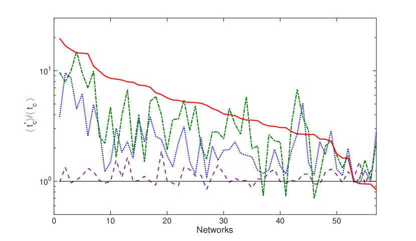
Figure 1: Relative increase in the time of consensus for the real-world networks studied according to different edge removal strategies. Red solid line: communicability angle; Green chained line: edge betweenness; Blue dotted line: Communicability; Magenta spaced broken line: random removal.

As can be seen from the Figure 1 the removal of 20% of the edges having the largest communicability angle increases the average time of consensus by a factor of $5.68\pm 4.32$. In other words, removing the edges with the largest angles multiplies by $5.68$ the time of consensus of the real-world networks studied. In 7 networks the average time of consensus is increased more than 10 times when the edges are removed according to the communicability angle, and in three cases the time of consensus is increased by more than 15 times.

The removal of the edges with the largest EBC also increases significantly the average time of consensus by a factor of $3.70\pm 2.87$. In only one case the time of consensus is increased by a factor of 10. In contrast, the random and independent removal of edges increases the time of consensus only by a factor of $1.12\pm 0.20$, and in no case the time of consensus is duplicated after the random removal of edges. The removal of the edges ranked according to the other indices studied here do not increase so significantly the time of consensus of the networks studied. For instance, removal of edges by the smallest communicability increases the average time of consensus by $2.41\pm 1.70$.

A significant difference among all the indices studied here is the fact that removing the edges by the smallest communicability angle decreases the average time of consensus of the networks. In general, the decrease of the time of consensus is not very dramatic—as average it decays by a factor of $0.96\pm 0.24$ respect to the original networks, but in some cases there is an acceleration of the consensus process by a factor of almost 2. This means that while the largest communicability angles identify those critical edges whose removal increase significantly the time of consensus, the smallest angles correspond to such edges which are redundant in the network and whose elimination in some way optimize the network for the consensus protocol. Care should be taken in considering such ’optimization’ of the network due to the fact that removal of these edges could make the networks more vulnerable to random failures.

So far we have presented the use of the EBC and the communicability angle based on an intuitive reasoning. As we have seen in the previous paragraphs this intuition has worked very well due to the fact that they identify critical edges for consensus dynamics in a very good way. Here we would like to present some mathematical justification for these empirical findings which will allow us to better understand the role of these structural parameters on the dynamical process studied. We first start with the EBC for which Comellas and Gago [26] have found the following lower bound. Let $EBC_{max}$ be the maximum of the EBC in a graph, then

$$EBC_{max}\geq\dfrac{n}{\sqrt{\mu_{2}\left(2\varDelta-\mu_{2}\right)}},$$ (25)

Consequently, the largest the EBC the smallest the algebraic connectivity, which implies that the average time of consensus increases according to (17). From the structural point of view this bound is probably telling us that the edges with the largest EBC are those bottlenecks (or bridges) connecting highly dense clusters of the network. Indeed, this is what the following bound obtained by Comellas and Gago indicates [26]:

$$EBC_{max}\geq\dfrac{n}{i\left(G\right)},$$ (26)

where $i\left(G\right)$ is the isoperimetric number defined as

$$i\left(G\right)=\inf_{S}\dfrac{\left|\partial S\right|}{\left|S\right|},$$ (27)

where $S$ is a subset of the set of nodes in the network (having less than the half of the total number of nodes) and $\partial S$ is the set of edges having one endpoint in $S$ and the other in its complement. Loosely speaking, a large isoperimetric number indicates that the network does not have structural bottlenecks, i.e., small sets of edges whose removal disconnect the graph into two almost identical components. Thus, the relation between EBC and $i\left(G\right)$ indicates that edges with large EBC are contained in networks with small isoperimetric number, i.e., containing structural bottlenecks.

Let us now turn our analysis to the communicability angle. We first consider a combined bound for the isoperimetric number obtained by Mohar [27]:

$$\dfrac{1}{2}\left(\delta-\lambda_{2}\right)\leq i\left(G\right)\leq\sqrt{\Delta^{2}-\lambda_{1}^{2}},$$ (28)

That is, the isoperimetric number increases with the increase of the largest eigenvalue $\lambda_{1}$, and with the decrease of the second largest eigenvalue of the adjacency matrix $\lambda_{2}$. We can resume this result by saying that the isoperimetric number increases with the increase of the spectral gap of the adjacency matrix, i.e., $\lambda_{1}-\lambda_{2}$. Let us consider what happen to the communicability angle between a pair of nodes when $\left(\lambda_{1}-\lambda_{2}\right)\rightarrow\infty$. In this case we have that

$$G_{pq}\rightarrow\psi_{1,p}\psi_{1,q}\exp\left(\lambda_{1}\right),\ \forall p,q\in V.$$ (29)

Thus, when $\left(\lambda_{1}-\lambda_{2}\right)\rightarrow\infty$ the communicability angle is

$$\theta_{pq}=\dfrac{G_{pq}}{\sqrt{G_{pp}G_{qq}}}\rightarrow\cos^{-1}1=0^{\circ}.$$ (30)

In other words, when the graph has large isoperimetric number the communicability angle tends to zero degrees. A large isoperimetric constant implies a large algebraic connectivity, i.e., $i\left(G\right)\leq\sqrt{\mu_{2}\left(2\varDelta-\mu_{2}\right)},$ [27], which indeed implies small average time of consensus.

6.2 Time of consensus and global network structure

Here we investigate how the global structure of networks influences the average time of consensus. In this case we are guided by the existence of analytic bounds for the algebraic connectivity of graphs. That is, the equation (17) indicates that the average time of consensus is bounded by the algebraic connectivity of the network. Thus, we should expect a nice correlation between these two parameters for networks. However, for a better understanding of this relation we should dig more deeply about the structural meaning of the algebraic connectivity. The algebraic connectivity is related to the minimum degree $\delta$ of a network via the following inequality:

$$\mu_{2}\left(G\right)\leq\dfrac{n\delta}{n-1}.$$ (31)

By combining two bounds obtained respectively by Alon and Milman [28] and by Mohar [29] we have that the algebraic connectivity is bounded as

$$\dfrac{4}{nDiam\left(G\right)}\leq\mu_{2}\left(G\right)\leq\dfrac{8\Delta}{Diam\left(G\right)^{2}}\log_{2}^{2}n.$$ (32)

We also consider a lower bound for the algebraic connectivity reported by Mohar [30] in terms of the average path length $\bar{l}\left(G\right)$ of the graph

$$\mu_{2}\left(G\right)\geq\dfrac{4}{2\left(n-1\right)\bar{l}\left(G\right)-\left(n-2\right)}.$$ (33)

These bounds clearly indicate a relation between the average time of consensus and the metrical properties of the networks.

There are many descriptors used to characterize the structure of graphs and networks [1]. Based on the analytic relations existing between the time of consensus and some structural parameters of networks we consider here a few network structural parameters to be correlated with the average time of consensus of networks. They include the average node degree

$$\bar{k}\left(G\right)=\frac{1}{n}\sum_{i=1}^{n}k_{i},$$ (34)

where $k_{i}$ is the degree of the corresponding node and the network density

$$\varrho\left(G\right)=\frac{\bar{k}}{n-1},$$ (35)

These parameters can be related to the algebraic connectivity via the bounds (31) and (32)—we remind that $\delta\leq\bar{k}\leq\Delta.$

On the other hand we consider the following metrical properties measured in terms of the shortest-path distance. They are the average shortest path length, which is given by

$$\bar{d}(G)=\frac{1}{n\left(n-1\right)}\sum_{u,v\in V}d(u,v),$$ (36)

and the network diameter, which is defined by

$$diam(G)=\max_{u,v\in V(G)}\left\{d(u,\,v)\right\}.$$ (37)

We also consider the average distance-sum index—a sort of average degree based on the sum of distances from a given node to every other node in the network,

$$s(G)=\dfrac{1}{n}\sum_{u\in V}s\left(u\right),$$ (38)

where $s\left(u\right)=\sum_{v}d(u,v)$.

We then obtain empirical correlations between these measures and the average time of consensus of all the real-world networks considered in this work. As expected the algebraic connectivity of the studied networks display a significant correlation with the average time of consensus with a Pearson correlation coefficient equal to $-0.792$. That is, an increase of the algebraic connectivity shorten the time of consensus of the network as expected from eq. (17). However, the Pearson correlation coefficient for the average time of consensus and the density is $-0.920$ and that with the average distance-sum is $0.967$ (see Fig. 2), indicating that these global structural parameters capture much better than the algebraic connectivity the structural influence over the consensus dynamics. These results can be understood in the following way. If we consider networks with the same number of nodes, then the influence of the algebraic connectivity over the dynamics is significantly larger. For instance, we have considered all the 11,117 connected graphs with 8 nodes and observed that the Pearson correlation coefficient between the time of consensus and $\mu_{2}$ is $-0.954$, while those with the density and average distance sum are $-0.755$ and $0.824$, respectively. As it can be seen from eq. (17) the number of nodes and the Fiedler vector $\vec{\psi}_{2}$ play also a fundamental role in the determination of the average time of consensus. Thus, in analyzing the influence of the global structure over the consensus dynamics, the network density and the average distance-sum play a more fundamental role than the algebraic connectivity. That is, increasing the density of the networks and reducing the average distance-sum of the nodes will decrease significantly the time of consensus, mainly as a consequence of the fact that information has significantly more ways to reach the same node from another using significantly shorter paths.

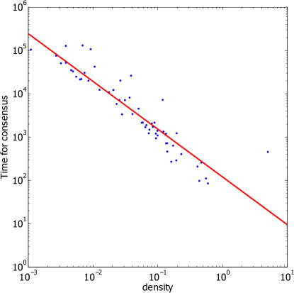
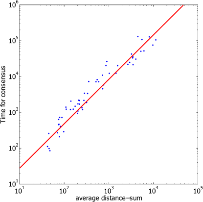
Figure 2: Illustration of the correlations between the average time of consensus for the real-world networks studied and the network density and average distance-sum.

7 Conclusions

We have investigated the relation between local and global structural parameters over the consensus dynamics on networks. At the local level we have identified the structural characteristics that make an edge critical for consensus. That is, those edges whose removal increases significantly the time necessary for a global consensus in a network. The removal of edges with the largest edge betweenness centrality, which accounts for the volume of information flowing through a given edge, increases the time of consensus in real-world networks by a factor of $3.70$. On the other hand, the removal of edges based on their largest communicability angles, which accounts for the quality of information transmitted through a given edge, increases the consensus time by a factor $5.68$. We have also considered some global structural parameters that influence the consensus dynamic of a network. In particular, the network density and the average distance-sum accounts for more than $80\%$ of the variance in the time of consensus of a large series of real-world networks arising in a variety of different scenarios. In closing, we have identified a few structural parameters—both local and global—which critically influence the dynamical properties of networks, allowing further studies to design networks with more efficient and robust consensus dynamics.

Appendix

Dataset-description

Biological networks

• Drosophila PIN: Protein-protein interaction network in Drosophila melanogaster (fruit fly).

• Hpyroli: Protein-protein interaction network in H. pyroli.

• KSHV: Protein-protein interaction network in Kaposi sarcoma herpes virus.

• Macaque: The brain network of macaque cortex.

• Malaria-PIN: Protein-protein interaction network in P. falciparum (malaria parasite).

• neurons: neuronal synaptic network of the nematode C. elegans. Included all data except muscle cells and using synaptic connections.

• PIN-Afulgidus: Protein-protein interaction network in A. fulgidus.

• PIN-Bsubtilis: Protein-protein interaction network in B. subtilis.

• PIN-Ecoli: Protein-protein interaction network in E. coli.

• Transc-yeast: Transcriptional regulation between genes in Saccaromyces cerevisiae.

• Trans-urchin: Developmental transcription network for sea urchin endomesoderm development.

• YeastS: Protein-protein interaction network in S. cerevisiae (yeast).

Ecological networks

• Benguela: Marine ecosystem of Bengela, off the south-west coast of South Africa.

• BridgeBrook: Pelagic species from the largest of set of fifty Adirondack Lake (NY) food webs.

• canton: Primarily invertebrates and algae in a tributary, surrounded by pasture, of the Taieri River in the South Island of New Zealand.

• Chesapeake: The pelagic portion of an eastern US estuary, with an emphasis on larger fish.

• Coachella: Wide range of highly aggregated taxa from the Coachella Valley desert in Southern California.

• ElVerde: Insects, spiders, birds, reptiles, and amphibians in a rainforest in Puerto Rico.

• grassland: All vascular plants and all insects and trophic interactions found inside stems of plants collected from 24 sites distributed within England and Wales

• ReefSmall: Caribbean coral reef ecosystem in Puerto Rico/Virgin Island shelf complex.

• ScotchBroom: Trophic interactions between the herbivores, parasitoids, predators, and pathogens associated with broom, Cytisus scoparius, collected in Silwood Park, Berkshire, England.

• Skipwith: Invertebrates in an English pond.

• StMarks: Mostly macroinvertebrates, fish, and birds associated with an estuarine seagrass community, Halodule wrightii, at the St. Marks Refuge, Florida, USA.

• StMartin: Birds and predators and arthropod prey of Anolis lizards on the island of St. Martin in the northern Lesser Antilles.

• Stony: Primarily invertebrates and algae in a tributary, surrounded by pasture, in native tussock habitat, of the Taieri River in the South Island of New Zealand.

• Ythan1: Mostly birds, fish, invertebrates, and metazona parasites in a Scottish estuary.

• Ythan2: Reduced version of Ythan1, without parasites.

Informational networks

• centrality-literature: Citation network of papers published in the field of Network Centrality.

• GD: Citation network of papers published in Proceedings of Graph Drawing during the period 1994-2000.

• Roget: Vocabulary network of words related by their definitions in Roget’s Thesaurus of the English language. Two words are connected if one is used in the definition of the other.

• SmallWorld: Citation network papers which cite Milgram’s 1967 Psychology Today paper or include Small World in the title.

Social networks

• BF (3, 70, 71): Networks of friendship ties from the communities identified as 23, 70, and 71 from the Brazilian Farmers longitudinal study on the adoption of a new corn seed.

• ColoSpg: The risk network of persons with HIV infection during its early epidemic phase in Colorado Springs, USA, using analysis of community-wide HIV/AIDS contact tracing records (sexual partners) during 1985-99.

• CorporatePeople: American corporate elite formed by the directors of the 625 largest corporations that reported the compositions of their boards, selected from the Fortune 1,000 in 1999.

• dolphins: Social network of a bottlenose dolphins (Tursiops truncates) population near New Zealand.

• Drugs: Social network of injecting drug-users (IDUs) who have shared a needle in the last six months.

• Galesburg2: Friendship ties among 31 physicians.

• High-tech: Friendship ties among the employees in a small high-tech computer firm which sells, installs, and maintains computer systems.

• hs_2: Heterosexual contacts, extracted at the Cadham Provincial Laboratory; a six-month block data from November 1997 to May 1998.

• Math Method: This network concerns the diffusion of a new mathematics method in the 1950s. It traces the diffusion of the modern mathematical method among school systems that combine elementary and secondary programs in Allegheny County (Pennsylvania, USA.) .

• PRISON: Social network of inmates in prison who chose “Which fellows on the tier are you closest friends with?”

• Sawmill: Social communication network within a sawmill, where employees were asked to indicate the frequency with which they discussed work matters with each of their colleagues.

• social3: Social network among college students participating in a course about leadership. The students choose which three members they want to have on a committee.

• Zackar: Social network of friendship between members of the Zackary karate club.

Technological networks

• electronic (1-3): Electronic sequential logic circuits parsed from the ISCAS89 benchmark set, where nodes represent logic gates and flip-flops.

• Internet-1997: The internet at the Autonomous System (AS) level, as of September 1997.

• Software (Abi, Digital, Mysql, VTK, XMMS): Software network development for different programs.

• USAir97: Airport transportation network between airports in the US in 1997.

			Relative increase of $\left\langle t_{c}\right\rangle$ according to:
No.	Network	$n$	$\widetilde{G}_{pq}$	EBC	$\theta_{pq}$	Rnd	Ref.
1	Coachella	30	3.83	9.68	19.68	0.71	[31]
2	Skipwith	35	9.52	7.89	16.85	0.76	[32]
3	electronic3	512	8.61	9.97	15.55	1.13	[33]
4	Software-XMMS	971	4.51	14.91	14.49	1.00	[70]
5	electronic2	252	6.22	9.52	14.43	0.93	[33]
6	hs_2	69	2.57	6.97	14.27	0.95	[34]
7	electronic1	122	4.95	9.95	11.00	1.03	[33]
8	Software-Mysql	1480	3.03	2.55	9.96	0.73	[70]
9	centrality-literature	118	1.23	2.21	8.98	0.81	[35]
10	Transc-yeast	662	1.48	4.70	8.54	1.08	[36]
11	social3	32	3.01	1.65	8.41	0.95	[34]
12	dolphins	62	1.82	3.94	8.25	0.79	[37]
13	StMarks	48	2.28	6.75	7.94	0.85	[38]
14	Drugs	616	1.62	1.79	7.87	0.97	[39]
15	Software-VTK	771	3.60	4.01	7.41	0.82	[70]
16	Malaria-PIN	229	2.27	1.50	7.36	1.23	[40]
17	CorporatePeople	1586	3.84	5.26	7.10	1.02	[41]
18	ElVerde	156	2.55	5.87	6.34	0.77	[42]
19	Math Method	30	2.39	3.99	6.08	0.85	[43]
20	Roget	994	1.72	1.92	5.69	0.96	[44]
21	PINEcoli	230	1.35	3.62	5.44	0.91	[45]
22	Benguela	29	2.24	3.66	5.39	0.72	[32]
23	Galesburg2	31	3.13	5.43	5.22	0.93	[46]
24	BridgeBrook	75	1.51	2.88	5.18	2.17	[47]
25	SmallWorld	233	1.16	4.81	5.15	1.00	[48]
26	PRISON	67	2.50	2.06	5.09	1.13	[49]
27	Stony	112	1.07	1.59	4.87	1.01	[50]
28	Hi-tech	33	2.08	2.80	4.56	0.60	[51]
29	Zackar	34	1.55	2.80	4.35	1.15	[52]
30	Software-Digital	150	1.91	2.41	4.07	1.33	[70]
31	Trans-Ecoli	328	1.94	4.57	4.00	0.72	[36]
32	GD	249	2.27	3.30	3.93	0.86	[48]
33	Hpyroli	710	1.79	2.67	3.70	0.63	[53]
34	ScotchBroom	154	1.72	5.78	3.58	0.98	[54]
35	canton	108	1.66	1.97	3.57	1.01	[55]
36	Chesapeake	33	1.26	2.08	3.54	1.55	[56]
37	Software-Abi	1035	1.18	0.74	3.28	0.62	[70]
38	BF-70	48	1.26	2.64	3.17	1.40	[57]
39	Sawmill	36	1.94	2.32	3.14	1.18	[58]
40	YeastS	2224	1.37	2.27	3.06	0.98	[59]
41	Ythan2	92	1.17	0.73	3.06	0.96	[61]
42	PIN-Ecoli	1251	1.90	3.32	2.82	0.96	[45]
43	Internet-1997	3015	2.67	6.76	2.68	0.99	[71]
44	Macaque	30	5.11	3.78	2.67	1.04	[72]
45	USAir97	332	1.47	2.88	2.65	0.90	[48]
46	Ythan1	134	1.14	0.70	2.65	0.97	[60]
47	neurons-A	280	2.27	1.14	2.41	0.70	[62]
48	grassland-A	75	1.75	2.08	2.41	0.97	[63]
49	BF-71	71	2.85	2.33	2.29	0.96	[57]
50	KSHV	50	1.29	1.71	1.77	0.79	[64]
51	Trans-urchin	45	1.13	1.32	1.62	0.78	[36]
52	BF-23	40	1.98	1.71	1.62	1.11	[57]
53	ColoSpg	324	1.03	0.98	1.00	0.99	[65]
54	PIN-Afulgidus	32	0.95	1.04	0.95	0.92	[66]
55	StMartin	44	1.26	1.55	0.95	0.83	[67]
56	Pin-Bsubtilis	84	0.98	1.04	0.94	0.96	[68]
57	ReefSmall	50	2.84	2.28	0.84	0.79	[69]

Table 1: Dataset: $n$ number of nodes, $\widetilde{G}_{pq}$ average communicability, EBC edge-betweenness centrality, $\theta_{pq}$ communicability angle, Rnd random. The largest increase in the average time of consensus are boldfaced.

References

- [1] E. Estrada, The Structure of complex networks. Theory and applications, (Oxford University Press, 2011).
- [2] M. Mesbahi, and M. Egerstedt, Graph Theoretic Methods in Multiagent Networks. (Princeton Series in Applied Mathematics, Princeton University Press, 2010).
- [3] R. Olfati-Saber, J. A. Fax, and R. M. Murray, Proc. IEEE, 95, (2007).
- [4] W. Ren, R. W. Beard, and E. M. Atkins, IEEE Control Syst. Mag. 27, 2, (2007).
- [5] J. Kenyeres, M. Kenyeres, M. Rupp, and P. Farkas, IEEE Proc. European Wireless Conference, April (2011).
- [6] Z. Dengchang, A. Zhulin, and X. Yongjun, Int. J. Distrib. Sens. N. 192128, (2013).
- [7] L. Lamport, Comm. ACM 21, 7 (1978).
- [8] N. T. Nguyen, Inform. Sciences 147, (2002).
- [9] J. Xie, S. Sreenivasan, G. Korniss, W. Zhang, C. Lim, and B. K. Szymanski, Phys. Rev. E 84, 011130, (2011).
- [10] D. Vilone, J. J. Ramasco, A. Sánchez, and M. San Miguel, Sci Rep 2, 686 (2012).
- [11] E. Mossel, and G. Schoenebeck, in Proceedings of 1st Symposium on ICS, January (2010).
- [12] J. R. G. Dyer, C. C. Ioannou, L. J. Morrel, D. P. Croft, I. D. Couzin, D. A. Waters, and J. Krause, Anim. Behav. 75, (2008).
- [13] Y. Liu, J. J. Slotine, and A. -L. Barabási, Nature 473, (2011).
- [14] M. Jalili, O. A., Sichani, and X. Yu, Phys. Rev. E 91, 012803 (2015).
- [15] P. Behavides, U. Diwekar, and H. Cabezas, J. Complex Networks, February (2015).
- [16] Z. Yuan, C. Zhao, Z. Di, W. X. Wang, and Y. C. Lai, Nat. Comm. 4, (2013).
- [17] M. Fiedler, Czech. Math. J. 23, 2 (1973).
- [18] N. M. M. de Abreu, Linear Algebra Appl. 423, 1 (2007).
- [19] M. Girvan, and M. E. J. Newman, PNAS 99, 12 (2002).
- [20] E. Estrada, and N. Hatano, Phys. Rev. E 77, 3 (2008).
- [21] E. Estrada, N. Hatano, and M. Benzi, Phys. Rep. 514, (2012).
- [22] E. Estrada, and N. Hatano, arXiv preprint arXiv:1412.7388 (2014).
- [23] E. Estrada, Linear Algebra Appl. 436, (2012) .
- [24] E. Estrada, Phys. Rev. E 85, 066122 (2012).
- [25] E. Estrada, M. G. Sánchez-Lirola, and J. A. de la Peña, Discrete Appl. Math. 176, (2014).
- [26] F. Comellas, and S. Gago, Linear Algebra Appl. 423, (2007).
- [27] B. Mohar, Linear Algebra Appl. 103, (1983).
- [28] N. Alon and V. D. Milman, J. Combin. Theory Ser. B 38, 1 (1985).
- [29] B. Mohar, Graph Theory, Combinatorics, and Applications, (Wiley, 1991), Vol. 2, pp. 871–898.
- [30] B. Mohar, Graph. Combinator, 7, 1 (1991).
- [31] P. H.Warren, Oikos 55, (1989).
- [32] P. Yodzis, Ecology 81, (2000).
- [33] R. Milo, S. Shen-Orr, S. Itzkovitz, N. Kashtan, D. Chklovskii, and U. Alon, Science 298, (2002).
- [34] L. D. Zeleny, Sociometry 13, 4 (1950).
- [35] N. P. Hummon, P. Doreian, and L. C. Freeman, Know. Creat. Difuss. Util. 11, (1990).
- [36] R. Milo, S. Itzkovitz, N. Kashtan, R. Levitt, S. Shen-Orr, I. Ayzenshtat, M. Sheffer, and U. Alon, Science 303, 5663 (2004).
- [37] D. Lusseau, K. Schneider, O. J. Boisseau, P. Haase, E. Slooten, and S. M. Dawson, Behav. Ecol. Sociobiol. 54, (2003)
- [38] L. Goldwasser, and J. A. Roughgarden, Ecology 74, (1993).
- [39] Data for this project was provided in part by NIH grants DA12831 and HD41877, those interested in obtaining a copy of these data should contact James Moody (moody.77@sociology.osu.edu).
- [40] D. LaCount, M. et. al. Nature 438, (2005).
- [41] G. F. Davis, M. Yoo, and W. E. Baker, Strategic Organization 1, (2003).
- [42] R. B. Waide, and D. A. Reagan, The Food Web of a Tropical Reinforest, (University Chicago Press, Chicago, 1996).
- [43] R. O. Carlson, Eugene: University of Oregon, Center for the Advanced Study of Educational Administration, (1965).
- [44] Roget’s thesaurus of english words and phrases, Project Gutenberg (2002), http://www.gutenberg.org/etxt/22.
- [45] G. Butland, et al. Nature 433, 7025 (2005).
- [46] J. S. Coleman, E. Katx, H. Menzel, Medical Innovation. A Diffusion Study, Indianapolis: Bobbs–Merrill Company (1966).
- [47] G. A. Polis, Am. Nat. 138, (1991).
- [48] V. Batagelj, and A. Mrvar, Graph Drawing Contest 2001, http://vlado.fmf.uni-lj.si/pub/networks/data/.
- [49] D. MacRae, Sociometry 23, (1960).
- [50] D. Baird, and R. E. Ulanowicz, Ecol. Mon. 59, (1989).
- [51] D. Krackhardt, Res. Sociol. Org. 16, (1999).
- [52] W. W. Zachary, J. Anthropol. Res. 33, (1977).
- [53] C. Lin, et al. Bioinformatics 21, (2005).
- [54] J. Memmott, N. D. Martinez, and J. E. Cohen, J. Anim. Ecol. 69, 1 (2000).
- [55] C. Townsend, R. M. Thompson, A. R. McIntosh, C. Kilroy, E. Edwards, and M. R. Scarsbrook, Ecol. Lett. 1, (1998).
- [56] R. R. Christian, and J. J. Luczkovich, Ecol. Model. 117, (1999).
- [57] W. A. Herzog et al., Patterns of Diffusion in Rural Brazil, Research Report, Rep. 10, (1968).
- [58] J. H. Michael, and J. G. Massey, Forest Prod. J. 47, (1997).
- [59] D. Bu, et al. Nucleic Acids Res. 31, (2003).
- [60] M. Huxman, S. Beany, and D. Raffaelli, Oikos 76, (1996).
- [61] S. J. Hall, and D. Rafaelli, J. Anim. Ecol. 60, (1991).
- [62] J. G. White, E. Southgate, J. N. Thomson, and S. Brenner, Philos. T. Roy. Soc. B 314, 1165 (1986).
- [63] N. D. Martinez, B. A. Hawkins, H. A. Dawah, and B. P. Feifarek, Ecology 80, (1999).
- [64] P. Uetz, et al. Science 311, (2006).
- [65] J. J. Potterat, L. Philips–Plummer, S. Q. Muth, R. B. Rothenberg, D. E. Woodhouse, T. S. Maldonado–Long, H. P. Zimmermann, and J. B. Muth, Transm. Infect. 78, (2002).
- [66] M. Motz, et al. J. Biol. Chem. 277, (2002).
- [67] N. D. Martinez, Ecol. Monogr. 61, (1991).
- [68] P. Noirot, and N. F. Noirot-Gross, Curr. Op. Microb. 7, (2004).
- [69] S. Opitz, ICLARM Tech. Rep. 43, Manila Philippines, (1996).
- [70] C. R. Mayers, Phys. Rev. E 68, 046116 (2003).
- [71] M. Faloutsos, P. Faloutsos, and C. Faloutsos, Comp. Comm. Rev. 29, (1999).
- [72] O. Sporns, and R. Kotter, PLoS Biol. 2, e369 (2004).