Twofold and Fourfold Symmetric Anisotropic Magnetoresistance Effect in A Model with Crystal Field

Abstract

We theoretically study the twofold and fourfold symmetric anisotropic magnetoresistance (AMR) effects of ferromagnets. We here use the two-current model for a system consisting of a conduction state and localized d states. The localized d states are obtained from a Hamiltonian with a spin–orbit interaction, an exchange field, and a crystal field. From the model, we first derive general expressions for the coefficient of the twofold symmetric term ($C_{2}$) and that of the fourfold symmetric term ($C_{4}$) in the AMR ratio. In the case of a strong ferromagnet, the dominant term in $C_{2}$ is proportional to the difference in the partial densities of states (PDOSs) at the Fermi energy ($E_{\mbox{\tiny F}}$) between the $d\varepsilon$ and $d\gamma$ states, and that in $C_{4}$ is proportional to the difference in the PDOSs at $E_{\mbox{\tiny F}}$ among the $d\varepsilon$ states. Using the dominant terms, we next analyze the experimental results for Fe₄N, in which $|C_{2}|$ and $|C_{4}|$ increase with decreasing temperature. The experimental results can be reproduced by assuming that the tetragonal distortion increases with decreasing temperature.

1 Introduction

The anisotropic magnetoresistance (AMR) effect is a phenomenon in which the electrical resistivity depends on the relative angle between the magnetization ($M$) direction and the electric current ($I$) direction (see Fig. 1). [1, 2, 3, 4, 5, 6, 7] The AMR effect has been studied extensively both experimentally and theoretically since 1857, when it was discovered by W. Thomson. [1] The AMR ratio, which is the efficiency of the effect, is generally defined by

$$\frac{\Delta\rho(\phi)}{\rho}=\frac{\rho(\phi)-\rho_{\perp}}{\rho_{\perp}},$$ (1)

with $\rho_{\perp}$=$\rho(\pi/2)$. Here, $\phi$ is the relative angle between the thermal average of the spin $\langle{\mbox{\boldmath$S$}}\rangle$ ($\propto$$-{\mbox{\boldmath$M$}}$) and $I$, and $\rho(\phi)$ is the resistivity at $\phi$.

Experimentally, $\Delta\rho(0)/\rho$ has been measured for various ferromagnets such as Fe,[4] Co,[4] Ni,[4] Ni-based alloys,[2] and half-metallic ferromagnets. [8, 10, 12, 13, 11, 9, 14, 15] In addition, the AMR ratios of many ferromagnets have been observed to be

$$\frac{\Delta\rho(\phi)}{\rho}=c_{0}+c_{2}\cos 2\phi,$$ (2)

where $c_{2}$ is the coefficient of the twofold symmetric term and $c_{0}$ is chosen to be $c_{2}$ so as to satisfy $\Delta\rho(\pi/2)/\rho$=0. [17, 10, 11, 16, 18]

Theoretically, expressions for $\Delta\rho(0)/\rho$ have often been derived by using electric transport theory based on the two-current model with $s$–$d$ scattering. [2, 3, 5, 6, 19, 20] The $s$–$d$ scattering means that the conduction electron (denoted as $s$) is scattered by impurities into the localized d states (denoted as $d$) with the exchange field and the spin–orbit interaction. As a representative study, Campbell, Fert, and Jaoul (CFJ)[2] derived an expression for $\Delta\rho(0)/\rho$ for strong ferromagnets[21] such as Ni-based alloys [see Eq. (116)]. On the basis of the CFJ model,[2] Malozemoff obtained an expression for $\Delta\rho(0)/\rho$ for weak ferromagnets[21] as well as strong ferromagnets.[5, 6] In addition, we extended the CFJ model[2] and the Malozemoff model [5, 6] to a more general model, which could systematically explain the experimental results of $\Delta\rho(0)/\rho$ for various ferromagnets including half-metallic ferromagnets.[19]

We also derived the analytic expression for $\Delta\rho(\phi)/\rho$ given by Eq. (2).[20] We then showed that the twofold symmetric feature of Eq. (2) could be intuitively explained by considering the d states distorted by the spin–orbit interaction. Note here that the crystal field of the d states was not taken into account in the derivation of Eq. (2). The d states were indexed by $M$=0, $\pm 1$, and $\pm 2$, with $M$ being the magnetic quantum number of the 3d states. Furthermore, the partial density of states (PDOS) of each d state at the Fermi energy ($E_{\mbox{\tiny F}}$) was assumed to be constant regardless of the d state.

Recently, the AMR ratios of several ferromagnets[22, 23, 24, 25, 26, 27, 28, 29, 30, 31] have been experimentally observed to be

$$\frac{\Delta\rho(\phi)}{\rho}=C_{0}+C_{2}\cos 2\phi+C_{4}\cos 4\phi.$$ (3)

Here, $C_{2}$ ($C_{4}$) is the coefficient of the twofold (fourfold) symmetric term, and $C_{0}$ is chosen to be $C_{2}-C_{4}$ so as to satisfy $\Delta\rho(\pi/2)/\rho$=0. For example, $|C_{2}|$ and $|C_{4}|$ for Fe₄N increase with decreasing temperature $T$ as shown later in Fig. 11.[22, 23, 24, 25, 26] The coefficients $C_{2}$ and $C_{4}$ were measured to be $C_{2}$=$-$0.0343 and $C_{4}$=0.00556 at $T$=4 K.[22]

The set of $C_{0}$, $C_{2}$, and $C_{4}$, however, has seldom been derived within the framework of transport theory and has often been represented by phenomenological expressions.[32, 33, 28, 27, 29] We anticipate that expressions for $C_{0}$, $C_{2}$, and $C_{4}$ obtained by transport theory will play an important role in the analysis and understanding of the AMR effect. We also predict that the fourfold symmetric term in Eq. (3) may appear under the crystal field of the d states, which was neglected in the previous models [19] [i.e., Eq. (2)].

In this paper, we obtained $C_{2}$ and $C_{4}$ by extending our model [19, 20] to one with a crystal field. We first performed a numerical calculation of $C_{2}$ and $C_{4}$ for a strong ferromagnet using the d states, which were obtained by applying the exact diagonalization method (EDM) to a Hamiltonian of the d states with a crystal field. The result revealed that $C_{4}$ appears under a crystal field of tetragonal symmetry, whereas it vanishes under a crystal field of cubic symmetry. We next derived general expressions for the resistivity, $C_{2}$, and $C_{4}$ for ferromagnets with the tetragonal field using the d states, which were obtained by applying first- and second-order perturbation theory (PT) to the Hamiltonian. From the expressions, we obtained expressions for $C_{2}$ and $C_{4}$ for the strong ferromagnet with the tetragonal field. The result showed that $C_{2}\cos 2\phi$ is related to the real part of the probability amplitudes of the specific hybridized states and $C_{4}\cos 4\phi$ is related to the probabilities of the specific hybridized states. In addition, we performed a simple analysis of the experimental results of $C_{2}$ and $C_{4}$ for Fe₄N using the dominant terms in $C_{2}$ and $C_{4}$ obtained by PT. The experimental results could be reproduced by assuming that the tetragonal distortion increases with decreasing $T$.

The present paper is organized as follows: In Sec. 2, we obtain wave functions of the localized d states by applying first- and second-order PT to the Hamiltonian of the localized d states. Using the wave functions, we derive general expressions for the resistivity, $C_{2}$, and $C_{4}$ for ferromagnets. In Sec. 3, we obtain expressions for $C_{2}$ and $C_{4}$ for a strong ferromagnet from the above-mentioned $C_{2}$ and $C_{4}$. In addition, we perform the numerical calculation of $C_{2}$ and $C_{4}$ using the d states, which are obtained by applying the EDM to the Hamiltonian. We then compare $C_{2}$ and $C_{4}$ obtained by PT and the respective values obtained by the EDM. In Sec. 4, we analyze the experimental results of $C_{2}$ and $C_{4}$ for Fe₄N. The conclusion is presented in Sec. 5. In Appendix A, we show the matrix of the Hamiltonian. In Appendix B, we give the zero-order states of the d states, which are obtained by performing the unitary transformation on the perturbation term. In Appendix C, we describe the overlap integrals of the $s$–$d$ scattering rate. In Appendix D, we give an expression for the $s$–$d$ scattering rate. Section E shows that the present $\Delta\rho(0)/\rho$ (=$2C_{2}$) coincides with our previous model[19, 20] and the CFJ model[2] under appropriate conditions.

2 Theory

In this section, we obtain general expressions for the resistivity, $C_{2}$, and $C_{4}$ in a model in which $I$ flows in the $x$ direction and $\langle{\mbox{\boldmath$S$}}\rangle$ ($\propto$$-{\mbox{\boldmath$M$}}$) lies in the $xy$ plane (see Fig. 1). We here use the two-current model with $s$–$d$ scattering in which the conduction electron is scattered into the localized d states by nonmagnetic impurities. [2, 3, 5, 6, 19, 20] The d states are obtained by applying PT to a Hamiltonian of the d states. We also explain the numerical calculation method for $C_{2}$ and $C_{4}$, in which the d states are obtained by applying the EDM to the Hamiltonian.

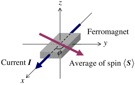
Figure 1: (Color online) Sketch of the sample geometry. The current $I$ flows in the $x$ direction, the thermal average of the spin $\langle{\mbox{\boldmath$S$}}\rangle$ ($\propto$$-{\mbox{\boldmath$M$}}$) lies in the $xy$ plane, and $\phi$ is the relative angle between the $I$ direction and the $\langle{\mbox{\boldmath$S$}}\rangle$ direction.

2.1 Hamiltonian

We first present the Hamiltonian ${\cal H}$ of the localized d states of a single atom [19, 34] in a ferromagnet with a spin–orbit interaction, an exchange field, and a crystal field of tetragonal symmetry. This crystal field represents the case that distortion in the $z$ direction is added to the crystal field of cubic symmetry.[35] Note that $C_{4}$ appears under a crystal field of tetragonal symmetry, whereas it vanishes under a crystal field of cubic symmetry, as will be described in Sec. 3.2.

The Hamiltonian ${\cal H}$ is expressed as

$${\cal H}={\cal H}_{0}+V,$$ (4)

$${\cal H}_{0}={\cal H}_{\rm cubic}-{\mbox{\boldmath$H$}}\cdot{\mbox{\boldmath$S$}},$$ (5)

$$V=V_{\rm so}+V_{\rm tetra},$$ (6)

with

$${\cal H}_{\rm cubic}=\sum_{\sigma=\pm}\Big{[}E_{\varepsilon}(|xy,\chi_{\sigma}(\phi)\rangle\langle xy,\chi_{\sigma}(\phi)|+|yz,\chi_{\sigma}(\phi)\rangle\langle yz,\chi_{\sigma}(\phi)|+|xz,\chi_{\sigma}(\phi)\rangle\langle xz,\chi_{\sigma}(\phi)|)$$

$$\hskip 42.67912pt+E_{\gamma}(|x^{2}-y^{2},\chi_{\sigma}(\phi)\rangle\langle x^{2}-y^{2},\chi_{\sigma}(\phi)|+|3z^{2}-r^{2},\chi_{\sigma}(\phi)\rangle\langle 3z^{2}-r^{2},\chi_{\sigma}(\phi)|)\Big{]},$$ (7)

$$V_{\rm so}=\lambda{\mbox{\boldmath$L$}}\cdot{\mbox{\boldmath$S$}},$$ (8)

$$V_{\rm tetra}=\sum_{\sigma=\pm}\Big{[}\delta_{\varepsilon}(|xz,\chi_{\sigma}(\phi)\rangle\langle xz,\chi_{\sigma}(\phi)|+|yz,\chi_{\sigma}(\phi)\rangle\langle yz,\chi_{\sigma}(\phi)|)$$

$$\hskip 34.14322pt+\delta_{\gamma}|3z^{2}-r^{2},\chi_{\sigma}(\phi)\rangle\langle 3z^{2}-r^{2},\chi_{\sigma}(\phi)|\Big{]},$$ (9)

and

$${\mbox{\boldmath$S$}}=(S_{x},S_{y},S_{z}),$$ (10)

$${\mbox{\boldmath$L$}}=(L_{x},L_{y},L_{z}),$$ (11)

$${\mbox{\boldmath$H$}}=H(\cos\phi,\sin\phi,0),$$ (12)

where $H>0$. Here, $S$ is the spin angular momentum and $L$ is the orbital angular momentum. The spin quantum number $S$ and the azimuthal quantum number $L$ are chosen to be $S$=1/2 and $L$=2.[19]

The above terms are explained as follows: The term ${\cal H}_{\rm cubic}$ represents the crystal field of cubic symmetry. The term $-{\mbox{\boldmath$H$}}\cdot{\mbox{\boldmath$S$}}$ is the Zeeman interaction due to the exchange field of the ferromagnet $H$, where $H$$\propto$$-{\mbox{\boldmath$M$}}$ and $H$$\propto$$\langle{\mbox{\boldmath$S$}}\rangle$. The term $V_{\rm so}$ is the spin–orbit interaction, where $\lambda$ is the spin–orbit coupling constant. The term $V_{\rm tetra}$ is an additional term to reproduce the crystal field of tetragonal symmetry. The state $|i,\chi_{\sigma}(\phi)\rangle$ is expressed by $|i,\chi_{\sigma}(\phi)\rangle$=$|i\rangle|\chi_{\sigma}(\phi)\rangle$. The state $|i\rangle$ is the orbital state, defined by $|xy\rangle$=$xyf(r)$, $|yz\rangle$=$yzf(r)$, $|xz\rangle$=$xzf(r)$, $|x^{2}-y^{2}\rangle$=$\frac{1}{2}(x^{2}-y^{2})f(r)$, and $|3z^{3}-r^{2}\rangle$=$\frac{1}{2\sqrt{3}}(3z^{2}-r^{2})f(r)$, with $f(r)$ being the radial part of the 3d orbital, where $r$=$\sqrt{x^{2}+y^{2}+z^{2}}$. The states $|xy\rangle$, $|yz\rangle$, and $|xz\rangle$ are referred to as $d\varepsilon$ orbitals and $|x^{2}-y^{2}\rangle$ and $|3z^{2}-r^{2}\rangle$ are referred to as $d\gamma$ orbitals. The quantity $E_{\varepsilon}$ is the energy level of $|xy\rangle$ and $E_{\gamma}$ is that of $|x^{2}-y^{2}\rangle$. The quantity $\Delta$ is defined as $\Delta$=$E_{\gamma}-E_{\varepsilon}$, $\delta_{\varepsilon}$ is the energy difference between $|xz\rangle$ (or $|yz\rangle$) and $|xy\rangle$, and $\delta_{\gamma}$ is that between $|3z^{2}-r^{2}\rangle$ and $|x^{2}-y^{2}\rangle$ (see Fig. 2). The state $|\chi_{\sigma}(\phi)\rangle$ ($\sigma$=$+$, $-$) is the spin state, i.e.,

$$|\chi_{+}(\phi)\rangle=\frac{1}{\sqrt{2}}(e^{-i\phi}|\uparrow\rangle+|\downarrow\rangle),$$ (13)

$$|\chi_{-}(\phi)\rangle=\frac{1}{\sqrt{2}}(-e^{-i\phi}|\uparrow\rangle+|\downarrow\rangle),$$ (14)

which are eigenstates of $-{\mbox{\boldmath$H$}}\cdot{\mbox{\boldmath$S$}}$. Here, $|\chi_{+}(\phi)\rangle$ ($|\chi_{-}(\phi)\rangle$) denotes the up spin state (down spin state) for the case that the quantization axis is chosen along the direction of $\langle{\mbox{\boldmath$S$}}\rangle$. The state $|\uparrow\rangle$ ($|\downarrow\rangle$) represents the up spin state (down spin state) for the case that the quantization axis is chosen along the $z$ axis.

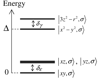
Figure 2: Energy levels of the 3d states in the crystal field of tetragonal symmetry. The energy levels are measured from $E_{\varepsilon}$.

Regarding the parameters, we assume the relations $\Delta/H\ll 1$, $|\lambda|/\Delta\ll 1$, $\delta_{\varepsilon}/\Delta\ll 1$, and $\delta_{\gamma}/\Delta\ll 1$, bearing a typical ferromagnet in mind. In particular, $H$, $\Delta$, and $|\lambda|$ are roughly set to $H$$\sim$1 eV, $\Delta$$\sim$0.1 eV, and $|\lambda|$$\sim$0.01 eV.[37, 36]

2.2 Wave functions of localized d states

To obtain the wave functions of the d states, we apply first- and second-order PT to ${\cal H}$ of Eq. (4). Here, ${\cal H}_{0}$ of Eq. (5) is the unperturbed term, while $V$ of Eq. (6) is the perturbed term. When the matrix of ${\cal H}$ is represented in the basis set $|xy,\chi_{\sigma}(\phi)\rangle$, $|yz,\chi_{\sigma}(\phi)\rangle$, $|xz,\chi_{\sigma}(\phi)\rangle$, $|x^{2}-y^{2},\chi_{\sigma}(\phi)\rangle$, and $|3z^{2}-r^{2},\chi_{\sigma}(\phi)\rangle$, the unperturbed system is degenerate (see Table 2 in Appendix A). We therefore use PT for the case that the unperturbed system is degenerate. [38, 39] First, the unitary transformation is performed for the subspace with the basis set $|xy,\chi_{\sigma}(\phi)\rangle$, $|yz,\chi_{\sigma}(\phi)\rangle$, and $|xz,\chi_{\sigma}(\phi)\rangle$ as mentioned in Appendix B. As a result, we obtain the zero-order states as $|\xi_{+},\chi_{+}(\phi)\rangle$, $|\delta_{\varepsilon},\chi_{+}(\phi)\rangle$, $|\xi_{-},\chi_{+}(\phi)\rangle$, $|\xi_{+},\chi_{-}(\phi)\rangle$, $|\delta_{\varepsilon},\chi_{-}(\phi)\rangle$, and $|\xi_{-},\chi_{-}(\phi)\rangle$. Here, $\xi_{\pm}$ and $\delta_{\varepsilon}$ represent the eigenvalues of $V$ in the above subspace, where $\xi_{\pm}$ is given by Eq. (91). The respective zero-order states are expressed as

$$|\xi_{+},\chi_{+}(\phi)\rangle=A\Big{[}(\delta_{\varepsilon}-\sqrt{\delta_{\varepsilon}^{2}+\lambda^{2}})|xy,\chi_{+}(\phi)\rangle+i\lambda\sin\phi|yz,\chi_{+}(\phi)\rangle-i\lambda\cos\phi|xz,\chi_{+}(\phi)\rangle\Big{]},$$

(15)

$$|\delta_{\varepsilon},\chi_{+}(\phi)\rangle=\cos\phi|yz,\chi_{+}(\phi)\rangle+\sin\phi|xz,\chi_{+}(\phi)\rangle,$$ (16)

$$|\xi_{-},\chi_{+}(\phi)\rangle=B\Big{[}(\delta_{\varepsilon}+\sqrt{\delta_{\varepsilon}^{2}+\lambda^{2}})|xy,\chi_{+}(\phi)\rangle+i\lambda\sin\phi|yz,\chi_{+}(\phi)\rangle-i\lambda\cos\phi|xz,\chi_{+}(\phi)\rangle\Big{]},$$

(17)

$$|\xi_{+},\chi_{-}(\phi)\rangle=A\Big{[}(\delta_{\varepsilon}-\sqrt{\delta_{\varepsilon}^{2}+\lambda^{2}})|xy,\chi_{-}(\phi)\rangle-i\lambda\sin\phi|yz,\chi_{-}(\phi)\rangle+i\lambda\cos\phi|xz,\chi_{-}(\phi)\rangle\Big{]},$$

(18)

$$|\delta_{\varepsilon},\chi_{-}(\phi)\rangle=\cos\phi|yz,\chi_{-}(\phi)\rangle+\sin\phi|xz,\chi_{-}(\phi)\rangle,$$ (19)

$$|\xi_{-},\chi_{-}(\phi)\rangle=B\Big{[}(\delta_{\varepsilon}+\sqrt{\delta_{\varepsilon}^{2}+\lambda^{2}})|xy,\chi_{-}(\phi)\rangle-i\lambda\sin\phi|yz,\chi_{-}(\phi)\rangle+i\lambda\cos\phi|xz,\chi_{-}(\phi)\rangle\Big{]},$$

with

$$A=(2\delta_{\varepsilon}^{2}+2\lambda^{2}-2\delta_{\varepsilon}\sqrt{\delta_{\varepsilon}^{2}+\lambda^{2}})^{-1/2},$$ (21)

$$B=(2\delta_{\varepsilon}^{2}+2\lambda^{2}+2\delta_{\varepsilon}\sqrt{\delta_{\varepsilon}^{2}+\lambda^{2}})^{-1/2}.$$ (22)

Next, using the basis set $|\xi_{+},\chi_{\pm}(\phi)\rangle$, $|\delta_{\varepsilon},\chi_{\pm}(\phi)\rangle$, $|\xi_{-},\chi_{\pm}(\phi)\rangle$, $|x^{2}-y^{2},\chi_{\pm}(\phi)\rangle$, and $|3z^{2}-r^{2},\chi_{\pm}(\phi)\rangle$, we construct the matrix of ${\cal H}$ of Eq. (4) as shown in Table 1. In the construction, we perform, for example, the following operations:

$$\lambda(L_{x}S_{x}+L_{y}S_{y})|\xi_{\pm},\chi_{-}(\phi)\rangle = \frac{1}{\sqrt{2\delta_{\varepsilon}^{2}+2\lambda^{2}\mp 2\delta_{\varepsilon}\sqrt{\delta_{\varepsilon}^{2}+\lambda^{2}}}}$$ (23)

$$\times\Bigg{\{}\frac{\sqrt{3}\lambda^{2}}{2}|3z^{2}-r^{2}\rangle(-i\cos 2\phi|\chi_{+}(\phi)\rangle-\sin 2\phi|\chi_{-}(\phi)\rangle)$$

$$+i\frac{\lambda^{2}}{2}|x^{2}-y^{2},\chi_{+}(\phi)\rangle-\frac{1}{2}\lambda^{2}|xy,\chi_{-}(\phi)\rangle$$

$$+i\frac{\lambda}{2}(\delta_{\varepsilon}\mp\sqrt{\delta_{\varepsilon}^{2}+\lambda^{2}})$$

$$\times[|xz\rangle(i\sin\phi|\chi_{+}(\phi)\rangle-\cos\phi|\chi_{-}(\phi)\rangle)$$

$$+|yz\rangle(i\cos\phi|\chi_{+}(\phi)\rangle+\sin\phi|\chi_{-}(\phi)\rangle)]\Bigg{\}},$$

$$\lambda(L_{x}S_{x}+L_{y}S_{y})|\delta_{\varepsilon},\chi_{-}(\phi)\rangle = i\frac{\sqrt{3}\lambda}{2}|3z^{2}-r^{2}\rangle(i\sin 2\phi|\chi_{+}(\phi)\rangle-\cos 2\phi|\chi_{-}(\phi)\rangle)$$ (24)

$$-i\frac{\lambda}{2}|x^{2}-y^{2},\chi_{-}(\phi)\rangle+\frac{\lambda}{2}|xy,\chi_{+}(\phi)\rangle.$$

Equations (23) and (24) play an important role in $C_{2}$ and $C_{4}$ as described in the $\phi$ dependence of the wave functions in this section.

Table 1: Matrix representation of ${\cal H}$ of Eq. (4) in the basis set $|\xi_{+},\chi_{+}(\phi)\rangle$, $|\delta_{\varepsilon},\chi_{+}(\phi)\rangle$, $|\xi_{-},\chi_{+}(\phi)\rangle$, $|\xi_{+},\chi_{-}(\phi)\rangle$, $|\delta_{\varepsilon},\chi_{-}(\phi)\rangle$, $|\xi_{-},\chi_{-}(\phi)\rangle$, $|x^{2}-y^{2},\chi_{+}(\phi)\rangle$, $|x^{2}-y^{2},\chi_{-}(\phi)\rangle$, $|3z^{2}-r^{2},\chi_{+}(\phi)\rangle$, and $|3z^{2}-r^{2},\chi_{-}(\phi)\rangle$. Here, $\xi_{\pm}$ is defined as $\xi_{\pm}$=$(\delta_{\varepsilon}\pm\sqrt{\delta_{\varepsilon}^{2}+\lambda^{2}})/2$ [see Eq. (91)]. In addition, $A$ and $B$ are given by Eqs. (21) and (22), respectively. In this table, $(\phi)$ in $\chi_{\sigma}(\phi)$ is omitted due to limited space.

	$|\xi_{+},\chi_{+}\rangle$	$|\delta_{\varepsilon},\chi_{+}\rangle$	$|\xi_{-},\chi_{+}\rangle$	$|\xi_{+},\chi_{-}\rangle$	$|\delta_{\varepsilon},\chi_{-}\rangle$	$|\xi_{-},\chi_{-}\rangle$	$|x^{2}-y^{2}$, $\chi_{+}\rangle$	$|x^{2}-y^{2}$, $\chi_{-}\rangle$	$|3z^{2}-r^{2}$, $\chi_{+}\rangle$	$|3z^{2}-r^{2}$, $\chi_{-}\rangle$
$\langle\xi_{+},\chi_{+}|$	$-\frac{H}{2}+\xi_{+}$	0	0	0	$\frac{\lambda A}{2}$	0	0	$-i\lambda A$	$-\frac{\sqrt{3}\lambda^{2}A}{2}$	$i\frac{\sqrt{3}\lambda^{2}A}{2}$
					$\times(2\xi_{-}-\lambda)$			$\times(2\xi_{-}+\frac{\lambda}{2})$	$\times\sin 2\phi$	$\times\cos 2\phi$
$\langle\delta_{\varepsilon},\chi_{+}|$	0	$-\frac{H}{2}+\delta_{\varepsilon}$	0	$\frac{\lambda A}{2}$	0	$\frac{\lambda B}{2}$	$-i\frac{\lambda}{2}$	0	$-i\frac{\sqrt{3}\lambda}{2}$	$\frac{\sqrt{3}\lambda}{2}$
				$\times(-2\xi_{-}+\lambda)$		$\times(-2\xi_{-}+\lambda)$			$\times\cos 2\phi$	$\times\sin 2\phi$
$\langle\xi_{-},\chi_{+}|$	0	0	$-\frac{H}{2}+\xi_{-}$	0	$\frac{\lambda B}{2}$	0	0	$-i\lambda B$	$-\frac{\sqrt{3}\lambda^{2}B}{2}$	$i\frac{\sqrt{3}\lambda^{2}B}{2}$
					$\times(2\xi_{+}-\lambda)$			$\times\left(2\xi_{+}+\frac{\lambda}{2}\right)$	$\times\sin 2\phi$	$\times\cos 2\phi$
$\langle\xi_{+},\chi_{-}|$	0	$\frac{\lambda A}{2}$	0	$\frac{H}{2}+\xi_{+}$	0	0	$-i\lambda A$	0	$i\frac{\sqrt{3}\lambda^{2}A}{2}$	$-\frac{\sqrt{3}\lambda^{2}A}{2}$
		$\times(-2\xi_{-}+\lambda)$					$\times\left(2\xi_{-}+\frac{\lambda}{2}\right)$		$\times\cos 2\phi$	$\times\sin 2\phi$
$\langle\delta_{\varepsilon},\chi_{-}|$	$\frac{\lambda A}{2}$	0	$\frac{\lambda B}{2}$	0	$\frac{H}{2}+\delta_{\varepsilon}$	0	0	$i\frac{\lambda}{2}$	$-\frac{\sqrt{3}\lambda}{2}$	$i\frac{\sqrt{3}\lambda}{2}$
	$\times(2\xi_{-}-\lambda)$		$\times(2\xi_{+}-\lambda)$						$\times\sin 2\phi$	$\times\cos 2\phi$
$\langle\xi_{-},\chi_{-}|$	0	$\frac{\lambda B}{2}$	0	0	0	$\frac{H}{2}+\xi_{-}$	$-i\lambda B$	0	$i\frac{\sqrt{3}\lambda^{2}B}{2}$	$-\frac{\sqrt{3}\lambda^{2}B}{2}$
		$\times(-2\xi_{-}+\lambda)$					$\times\left(2\xi_{+}+\frac{\lambda}{2}\right)$		$\times\cos 2\phi$	$\times\sin 2\phi$
$\langle x^{2}-y^{2}$, $\chi_{+}|$	0	$i\frac{\lambda}{2}$	0	$i\lambda A$	0	$i\lambda B$	$-\frac{H}{2}+\Delta$	0	0	0
				$\times\left(2\xi_{-}+\frac{\lambda}{2}\right)$		$\times\left(2\xi_{+}+\frac{\lambda}{2}\right)$
$\langle x^{2}-y^{2}$, $\chi_{-}|$	$i\lambda A$	0	$i\lambda B$	0	$-i\frac{\lambda}{2}$	0	0	$\frac{H}{2}+\Delta$	0	0
	$\times\left(2\xi_{-}+\frac{\lambda}{2}\right)$		$\times\left(2\xi_{+}+\frac{\lambda}{2}\right)$
$\langle 3z^{2}-r^{2}$, $\chi_{+}|$	$-\frac{\sqrt{3}\lambda^{2}A}{2}$	$i\frac{\sqrt{3}\lambda}{2}$	$-\frac{\sqrt{3}\lambda^{2}B}{2}$	$-i\frac{\sqrt{3}\lambda^{2}A}{2}$	$-\frac{\sqrt{3}\lambda}{2}$	$-i\frac{\sqrt{3}\lambda^{2}B}{2}$	0	0	$-\frac{H}{2}+\Delta+\delta_{\gamma}$	0
	$\times\sin 2\phi$	$\times\cos 2\phi$	$\times\sin 2\phi$	$\times\cos 2\phi$	$\times\sin 2\phi$	$\times\cos 2\phi$
$\langle 3z^{2}-r^{2}$, $\chi_{-}|$	$-i\frac{\sqrt{3}\lambda^{2}A}{2}$	$\frac{\sqrt{3}\lambda}{2}$	$-i\frac{\sqrt{3}\lambda^{2}B}{2}$	$-\frac{\sqrt{3}\lambda^{2}A}{2}$	$-i\frac{\sqrt{3}\lambda}{2}$	$-\frac{\sqrt{3}\lambda^{2}B}{2}$	0	0	0	$\frac{H}{2}+\Delta+\delta_{\gamma}$
	$\times\cos 2\phi$	$\times\sin 2\phi$	$\times\cos 2\phi$	$\times\sin 2\phi$	$\times\cos 2\phi$	$\times\sin 2\phi$

Applying the usual first- and second-order PT to ${\cal H}$ in Table 1, we obtain $|i,\chi_{\varsigma}(\phi))$, where $i$ ($\varsigma$) denotes the orbital index (spin index) of the dominant state in $|i,\chi_{\varsigma}(\phi))$. The d state of the up spin $|i,\chi_{+}(\phi))$ is expressed as

$$|\xi_{+},\chi_{+}(\phi)) = c_{\xi_{+},+}(|x^{2}-y^{2},\chi_{-}(\phi)\rangle+w^{\xi_{+},+}_{3z^{2}-r^{2},+}\sin 2\phi|3z^{2}-r^{2},\chi_{+}(\phi)\rangle$$ (25)

$$+w^{\xi_{+},+}_{3z^{2}-r^{2},-}\cos 2\phi|3z^{2}-r^{2},\chi_{-}(\phi)\rangle)\ldots~{},$$

$$|\delta_{\varepsilon},\chi_{+}(\phi)) = c_{\delta_{\varepsilon},+}(|x^{2}-y^{2},\chi_{+}(\phi)\rangle+w^{\delta_{\varepsilon},+}_{3z^{2}-r^{2},+}\cos 2\phi|3z^{2}-r^{2},\chi_{+}(\phi)\rangle$$ (26)

$$+w^{\delta_{\varepsilon},+}_{3z^{2}-r^{2},-}\sin 2\phi|3z^{2}-r^{2},\chi_{-}(\phi)\rangle)\ldots~{},$$

$$|\xi_{-},\chi_{+}(\phi)) = c_{\xi_{-},+}(|x^{2}-y^{2},\chi_{-}(\phi)\rangle+w^{\xi_{-},+}_{3z^{2}-r^{2},+}\sin 2\phi|3z^{2}-r^{2},\chi_{+}(\phi)\rangle$$ (27)

$$+w^{\xi_{-},+}_{3z^{2}-r^{2},-}\cos 2\phi|3z^{2}-r^{2},\chi_{-}(\phi)\rangle)\ldots~{},$$

$$|x^{2}-y^{2},\chi_{+}(\phi)) = c_{x^{2}-y^{2},+}(|x^{2}-y^{2},\chi_{+}(\phi)\rangle+w^{x^{2}-y^{2},+}_{3z^{2}-r^{2},+}\cos 2\phi|3z^{2}-r^{2},\chi_{+}(\phi)\rangle)\ldots~{},$$

$$|3z^{2}-r^{2},\chi_{+}(\phi)) = c_{3z^{2}-r^{2},+}(|3z^{2}-r^{2},\chi_{+}(\phi)\rangle+w^{3z^{2}-r^{2},+}_{x^{2}-y^{2},+}\cos 2\phi|x^{2}-y^{2},\chi_{+}(\phi)\rangle)\ldots~{},$$

and the d state of the down spin $|i,\chi_{-}(\phi))$ is expressed as

$$|\xi_{+},\chi_{-}(\phi)) = c_{\xi_{+},-}(|x^{2}-y^{2},\chi_{+}(\phi)\rangle+w^{\xi_{+},-}_{3z^{2}-r^{2},+}\cos 2\phi|3z^{2}-r^{2},\chi_{+}(\phi)\rangle$$ (30)

$$+w^{\xi_{+},-}_{3z^{2}-r^{2},-}\sin 2\phi|3z^{2}-r^{2},\chi_{-}(\phi)\rangle)\ldots~{},$$

$$|\delta_{\varepsilon},\chi_{-}(\phi)) = c_{\delta_{\varepsilon},-}(|x^{2}-y^{2},\chi_{-}(\phi)\rangle+w^{\delta_{\varepsilon},-}_{3z^{2}-r^{2},+}\sin 2\phi|3z^{2}-r^{2},\chi_{+}(\phi)\rangle$$ (31)

$$+w^{\delta_{\varepsilon},-}_{3z^{2}-r^{2},-}\cos 2\phi|3z^{2}-r^{2},\chi_{-}(\phi)\rangle)\ldots~{},$$

$$|\xi_{-},\chi_{-}(\phi)) = c_{\xi_{-},-}(|x^{2}-y^{2},\chi_{+}(\phi)\rangle+w^{\xi_{-},-}_{3z^{2}-r^{2},+}\cos 2\phi|3z^{2}-r^{2},\chi_{+}(\phi)\rangle$$ (32)

$$+w^{\xi_{-},-}_{3z^{2}-r^{2},-}\sin 2\phi|3z^{2}-r^{2},\chi_{-}(\phi)\rangle)\ldots~{},$$

$$|x^{2}-y^{2},\chi_{-}(\phi)) = c_{x^{2}-y^{2},-}(|x^{2}-y^{2},\chi_{-}(\phi)\rangle+w^{x^{2}-y^{2},-}_{3z^{2}-r^{2},-}\cos 2\phi|3z^{2}-r^{2},\chi_{-}(\phi)\rangle)\ldots~{},$$

$$|3z^{2}-r^{2},\chi_{-}(\phi)) = c_{3z^{2}-r^{2},-}(|3z^{2}-r^{2},\chi_{-}(\phi)\rangle+w^{3z^{2}-r^{2},-}_{x^{2}-y^{2},-}\cos 2\phi|x^{2}-y^{2},\chi_{-}(\phi)\rangle)\ldots~{}.$$

In the right-hand side of Eqs. (25)$-$(2.2), we specify only the $|3z^{2}-r^{2},\chi_{\sigma}(\phi)\rangle$ and $|x^{2}-y^{2},\chi_{\sigma}(\phi)\rangle$ terms because these states contribute to the present transport in which $I$ flows in the $x$ direction (see Appendix C). The dominant states in $|\xi_{+},\chi_{\sigma}(\phi))$, $|\delta_{\varepsilon},\chi_{\sigma}(\phi))$, $|\xi_{-},\chi_{\sigma}(\phi))$, $|x^{2}-y^{2},\chi_{\sigma}(\phi))$, and $|3z^{2}-r^{2},\chi_{\sigma}(\phi))$ are respectively written as $|\xi_{+},\chi_{\sigma}(\phi)\rangle$, $|\delta_{\varepsilon},\chi_{\sigma}(\phi)\rangle$, $|\xi_{-},\chi_{\sigma}(\phi)\rangle$, $|x^{2}-y^{2},\chi_{\sigma}(\phi)\rangle$, and $|3z^{2}-r^{2},\chi_{\sigma}(\phi)\rangle$, although they are not shown in Eqs. (25)$-$(27) and (30)$-$(32). The other states, except for the dominant state in each $|i,\chi_{\varsigma}(\phi))$, represent the slightly hybridized states due to the spin–orbit interaction. The quantity $w^{i,\varsigma}_{j,\sigma}\cos 2\phi$ or $w^{i,\varsigma}_{j,\sigma}\sin 2\phi$ represents the probability amplitude of $|j,\chi_{\sigma}(\phi)\rangle$ normalized by $c_{i,\varsigma}$. Here, $w^{i,\varsigma}_{j,\sigma}$ is the coefficient of the $\cos 2\phi$ or $\sin 2\phi$ term normalized by $c_{i,\varsigma}$, while $c_{i,\varsigma}$ is the coefficient of the constant term, which does not depend on $\phi$. Such $w^{i,\varsigma}_{j,\sigma}\cos 2\phi$ and $w^{i,\varsigma}_{j,\sigma}\sin 2\phi$ generate the twofold and fourfold symmetric terms of $\Delta\rho(\phi)/\rho$ as described in Sec. 2.5.

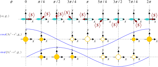
(a)

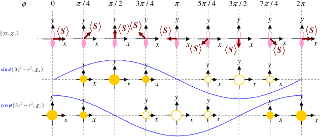
(b)

Figure 3: (Color online) (a) Schematic illustration of the $\phi$ dependences of $|xz,\chi_{-}(\phi)\rangle$, $\cos\phi|3z^{2}-r^{2},\chi_{+}(\phi)\rangle$, and $\sin\phi|3z^{2}-r^{2},\chi_{-}(\phi)\rangle$ in $\lambda L_{y}S_{y}|xz,\chi_{-}(\phi)\rangle$ of Eq. (A). The upper part shows the top view (looking down along the $z$ axis) of $|xz,\chi_{-}(\phi)\rangle$. The middle part shows $\cos\phi|3z^{2}-r^{2},\chi_{+}(\phi)\rangle$ in the $xy$ plane. The lower part shows $\sin\phi|3z^{2}-r^{2},\chi_{-}(\phi)\rangle$ in the $xy$ plane. Here, $|xz,\chi_{-}(\phi)$ is shown by the sky-blue or sky-blue-bordered orbital and $|3z^{2}-r^{2},\chi_{\pm}(\phi)\rangle$ is shown by the yellow or yellow-bordered orbital. The blue curve in the middle part is $\cos\phi$ and that in the lower part is $\sin\phi$. Note that the $\phi$ dependent coefficients of $|3z^{2}-r^{2},\chi_{\pm}(\phi)\rangle$ are given by only $\cos\phi$ and $\sin\phi$; that is, the prefactor of $\cos\phi$ or $\sin\phi$ is ignored. In addition, the color-filled orbitals (white orbitals with a colored border) express regions with a negative sign (positive sign) in the wave function, where the $\phi$ dependent coefficients are taken into consideration in regard to $|3z^{2}-r^{2},\chi_{\pm}(\phi)\rangle$. (b) Schematic illustration of the $\phi$ dependences of $|yz,\chi_{-}(\phi)\rangle$, $\sin\phi|3z^{2}-r^{2},\chi_{+}(\phi)\rangle$, and $\cos\phi|3z^{2}-r^{2},\chi_{-}(\phi)\rangle$ in $\lambda L_{x}S_{x}|yz,\chi_{-}(\phi)\rangle$ of Eq. (A). The upper part shows the top view (looking down along the $z$ axis) of $|yz,\chi_{-}(\phi)\rangle$. The middle part shows $\sin\phi|3z^{2}-r^{2},\chi_{+}(\phi)\rangle$ in the $xy$ plane. The lower part shows $\cos\phi|3z^{2}-r^{2},\chi_{-}(\phi)\rangle$ in the $xy$ plane. Here, $|yz,\chi_{-}(\phi)\rangle$ is shown by the pink or pink-bordered orbital. The blue curve in the middle part is $\sin\phi$ and that in the lower part is $\cos\phi$. The other notation is the same as in (a).

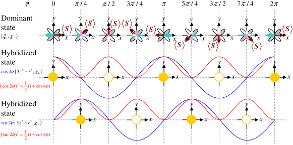
(a)

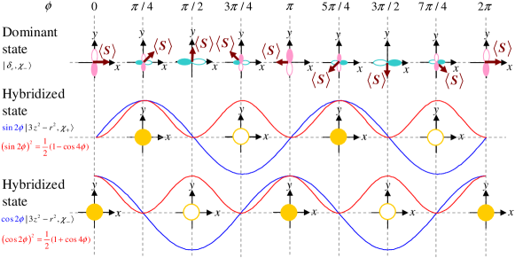
(b)

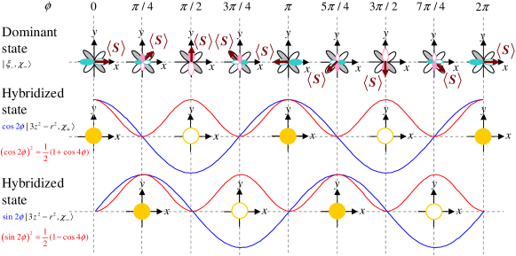
(c)

Figure 4: (Color online) Schematic illustration of the $\phi$ dependences of the dominant states in $d\varepsilon$ states and the hybridized states in Eqs. (30)$-$(32). The dominant states in (a), (b), and (c) are $|\xi_{+},\chi_{-}(\phi)\rangle$ of Eq. (2.2), $|\delta_{\varepsilon},\chi_{-}(\phi)\rangle$ of Eq. (19), and $|\xi_{-},\chi_{-}(\phi)\rangle$ of Eq. (2.2), respectively. The hybridized states are represented by expressions with a probability amplitude of $\cos 2\phi$ or $\sin 2\phi$, i.e., $\cos 2\phi|3z^{2}-r^{2},\chi_{\pm}(\phi)\rangle$ and $\sin 2\phi|3z^{2}-r^{2},\chi_{\pm}(\phi)\rangle$, where the prefactor of $\cos 2\phi$ or $\sin 2\phi$ is ignored. In each panel, the upper part shows the top view (looking down along the $z$ axis) of the dominant state. In (a) and (c), the middle part shows $\cos 2\phi|3z^{2}-r^{2},\chi_{+}(\phi)\rangle$ in the $xy$ plane, and the lower part shows $\sin 2\phi|3z^{2}-r^{2},\chi_{-}(\phi)\rangle$ in the $xy$ plane. In (b), the middle part shows $\sin 2\phi|3z^{2}-r^{2},\chi_{-}(\phi)\rangle$ in the $xy$ plane, and the lower part shows $\cos 2\phi|3z^{2}-r^{2},\chi_{+}(\phi)\rangle$ in the $xy$ plane. The state $|yz,\chi_{-}(\phi)\rangle$ is shown by the pink or pink-bordered orbital, $|xz,\chi_{-}(\phi)\rangle$ is shown by the sky-blue or sky-blue-bordered orbital, and $|xy,\chi_{-}(\phi)\rangle$ is shown by the gray or gray-bordered orbital. The state $|3z^{2}-r^{2},\chi_{-}(\phi)\rangle$ is represented by the yellow or yellow-bordered orbital. The color-filled orbitals (white orbitals with a colored border) express regions with a negative sign (positive sign) in the wave function including the probability amplitude. In the middle part of (a) and (c) and the lower part of (b), the blue and red curves are $\cos 2\phi$ and $\cos^{2}2\phi$ [=$(1+\cos 4\phi)/2$], respectively. In the lower parts of (a) and (c) and the middle part of (b), the blue and red curves are $\sin 2\phi$ and $\sin^{2}2\phi$ [=$(1-\cos 4\phi)/2$], respectively.

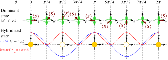
(a)

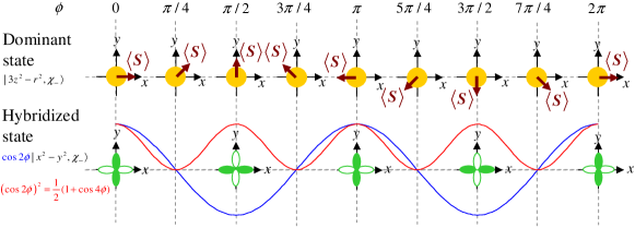
(b)

Figure 5: (Color online) Schematic illustration of the $\phi$ dependences of the dominant states in $d\gamma$ states and the hybridized states in Eqs. (2.2) and (2.2). The dominant states in (a) and (b) are $|x^{2}-y^{2},\chi_{-}(\phi)\rangle$ and $|3z^{2}-y^{2},\chi_{-}(\phi)\rangle$, respectively. The hybridized states are represented by expressions with a probability amplitude of $\cos 2\phi$, i.e., $\cos 2\phi|3z^{2}-r^{2},\chi_{-}(\phi)\rangle$ and $\cos 2\phi|x^{2}-y^{2},\chi_{-}(\phi)\rangle$, where the prefactor of $\cos 2\phi$ is ignored. In each panel, the upper part shows the top view (looking down along the $z$ axis) of the dominant state. In (a), the lower part shows $\cos 2\phi|3z^{2}-r^{2},\chi_{-}(\phi)\rangle$ in the $xy$ plane. In (b), the lower part shows $\sin 2\phi|x^{2}-y^{2},\chi_{-}(\phi)\rangle$ in the $xy$ plane. The state $|3z^{2}-r^{2},\chi_{-}(\phi)\rangle$ is shown by the yellow or yellow-bordered orbital. The state $|x^{2}-y^{2},\chi_{-}(\phi)\rangle$ is shown by the green or green-bordered orbital. The color-filled orbitals (white orbitals with a colored border) express regions with a negative sign (positive sign) in the wave function, where the probability amplitude is taken into consideration in regard to $|3z^{2}-r^{2},\chi_{-}(\phi)\rangle$ and $|x^{2}-y^{2},\chi_{-}(\phi)\rangle$. In the lower parts of (a) and (b), the blue and red curves are $\cos 2\phi$ and $\cos^{2}2\phi$ [=$(1+\cos 4\phi)/2$], respectively.

2.3 Origin of $\cos 2\phi$ and $\sin 2\phi$ terms in d states

We explain the origin of the $\cos 2\phi$ and $\sin 2\phi$ terms in Eqs. (25)$-$(2.2). In the $d\varepsilon$ states, the $\cos 2\phi$ and $\sin 2\phi$ terms appear through $d\varepsilon-d\gamma$ hybridization. In the $d\gamma$ states, they appear owing to $d\gamma-d\varepsilon-d\gamma^{\prime}$ hybridization, in which the $d\gamma$ states are hybridized to the $d\gamma^{\prime}$ states via the $d\varepsilon$ states. These hybridizations are due to the specific matrix elements in Table 1, i.e., $\langle 3z^{2}-r^{2},\chi_{\sigma^{\prime}}(\phi)|{\cal H}|\xi_{\pm},\chi_{\sigma}(\phi)\rangle$ and $\langle 3z^{2}-r^{2},\chi_{\sigma^{\prime}}(\phi)|{\cal H}|\delta_{\varepsilon},\chi_{\sigma}(\phi)\rangle$, with $\sigma$=$+$, $-$ and $\sigma^{\prime}$=$+$, $-$. We now focus on $\langle 3z^{2}-r^{2},\chi_{\sigma^{\prime}}(\phi)|{\cal H}|\xi_{\pm},\chi_{-}(\phi)\rangle$ and $\langle 3z^{2}-r^{2},\chi_{\sigma^{\prime}}(\phi)|{\cal H}|\delta_{\varepsilon},\chi_{-}(\phi)\rangle$, where $\langle 3z^{2}-r^{2},\chi_{\sigma^{\prime}}(\phi)|{\cal H}|\xi_{\pm},\chi_{+}(\phi)\rangle$ and $\langle 3z^{2}-r^{2},\chi_{\sigma^{\prime}}(\phi)|{\cal H}|\delta_{\varepsilon},\chi_{+}(\phi)\rangle$ can also be discussed in a similar way. These matrix elements originate from only the $\cos 2\phi$ and $\sin 2\phi$ terms in Eqs. (23) and (24). Here, $\cos 2\phi$ and $\sin 2\phi$ are formed by the multiplication of the following coefficients:

1. The $\phi$ dependent coefficients of $|3z^{2}-r^{2},\chi_{-}(\phi)\rangle$ in $\lambda L_{y}S_{y}|xz,\chi_{-}(\phi)\rangle$ of Eq. (A) and $\lambda L_{x}S_{x}|yz,\chi_{-}(\phi)\rangle$ of Eq. (A).

   Note that the $\phi$ dependent coefficients of $|x^{2}-y^{2},\chi_{-}(\phi)\rangle$ in Eqs. (A) and (A) are not responsible for the $\cos 2\phi$ and $\sin 2\phi$ terms in Eqs. (23) and (24).

2. The $\phi$ dependent coefficients of $|xz,\chi_{-}(\phi)\rangle$ and $|yz,\chi_{-}(\phi)\rangle$ in Eqs. (2.2)$-$(2.2).

We discuss (i). We first emphasize that the operations that generate $|3z^{2}-r^{2},\chi_{\sigma}(\phi)\rangle$ are $\lambda L_{y}S_{y}|xz,\chi_{-}(\phi)\rangle$ of Eq. (A) and $\lambda L_{x}S_{x}|yz,\chi_{-}(\phi)\rangle$ of Eq. (A). In Fig. 3(a), we show the $\phi$ dependences of $\cos\phi|3z^{2}-r^{2},\chi_{+}(\phi)\rangle$ and $\sin\phi|3z^{2}-r^{2},\chi_{-}(\phi)\rangle$ in $\lambda L_{y}S_{y}|xz,\chi_{-}(\phi)\rangle$ of Eq. (A). Here, the coefficients of $|3z^{2}-r^{2},\chi_{\pm}(\phi)\rangle$ are given by only $\cos\phi$ and $\sin\phi$; that is, the prefactor of $\cos\phi$ or $\sin\phi$ is ignored for simplicity. When $\phi$=0, the coefficient of $|3z^{2}-r^{2},\chi_{+}(0)\rangle$ is finite, whereas that of $|3z^{2}-r^{2},\chi_{-}(0)\rangle$ is zero. In brief, since the spin direction of $|\chi_{-}(0)\rangle$ in $|xz,\chi_{-}(0)\rangle$ is the $x$ direction, $S_{y}|\chi_{-}(0)\rangle$ becomes $S_{y}|\chi_{-}(0)\rangle$ =$-\frac{i}{2}|\chi_{+}(0)\rangle$. Namely, the spin is reversed by the operation of $S_{y}$. In contrast, when $\phi$=$\pi/2$, the coefficient of $|3z^{2}-r^{2},\chi_{-}(\pi/2)\rangle$ is finite, whereas that of $|3z^{2}-r^{2},\chi_{+}(\pi/2)\rangle$ is zero. In short, since the spin direction of $|\chi_{-}(\pi/2)\rangle$ in $|xz,\chi_{-}(\pi/2)\rangle$ is the $y$ direction, $S_{y}|\chi_{-}(\pi/2)\rangle$ becomes $S_{y}|\chi_{-}(\pi/2)\rangle$ =$-\frac{1}{2}|\chi_{-}(\pi/2)\rangle$. Namely, the spin is conserved under the operation of $S_{y}$. In a similar way, we can consider the $\phi$ dependence of the coefficient of $|3z^{2}-r^{2},\chi_{\pm}(\phi)\rangle$ in $\lambda L_{x}S_{x}|yz,\chi_{-}(\phi)\rangle$ of Eq. (A) [also see Fig. 3(b)].

2.4 Illustration of d states

In Figs. 4 and 5, we show schematic illustrations of the $\phi$ dependences of the dominant states and hybridized states in Eqs. (30)$-$(2.2). The dominant states are $|\xi_{+},\chi_{-}(\phi)\rangle$ of Eq. (2.2), $|\delta_{\varepsilon},\chi_{-}(\phi)\rangle$ of Eq. (19), $|\xi_{-},\chi_{-}(\phi)\rangle$ of Eq. (2.2), $|x^{2}-y^{2},\chi_{-}(\phi)\rangle$, and $|3z^{2}-r^{2},\chi_{-}(\phi)\rangle$. The hybridized states are represented by expressions with a probability amplitude of $\cos 2\phi$ or $\sin 2\phi$, i.e., $\cos 2\phi|3z^{2}-r^{2},\chi_{\pm}(\phi)\rangle$, $\sin 2\phi|3z^{2}-r^{2},\chi_{\pm}(\phi)\rangle$, and $\cos 2\phi|x^{2}-y^{2},\chi_{-}(\phi)\rangle$, where the prefactor of $\cos 2\phi$ or $\sin 2\phi$ is ignored for simplicity. Each probability is also given by $\cos^{2}2\phi$ [=$(1+\cos 4\phi)/2$] or $\sin^{2}2\phi$ [=$(1-\cos 4\phi)/2$]. Such $\phi$ dependences originate from the $\phi$ dependent coefficients of $|3z^{2}-r^{2},\chi_{\sigma}(\phi)\rangle$ in $\lambda(L_{x}S_{x}+L_{y}S_{y})|\xi_{\pm},\chi_{-}(\phi)\rangle$ of Eq. (23) and $\lambda(L_{x}S_{x}+L_{y}S_{y})|\delta_{\varepsilon},\chi_{-}(\phi)\rangle$ of Eq. (24). These operations are commented on as follows:

1. $\lambda(L_{x}S_{x}+L_{y}S_{y})|\xi_{\pm},\chi_{-}(\phi)\rangle$ of Eq. (23)
   When $\phi$=0, only $\lambda L_{y}S_{y}|xz,\chi_{-}(0)\rangle$ in this operation generates $|3z^{2}-r^{2},\chi_{+}(0)\rangle$ [see the case of $\phi$=0 in Figs. 4(a) and 4(c)]. This feature comes from the case of $\phi$=0 in Fig. 3(a). When $\phi$=$\pi/2$, only $\lambda L_{x}S_{x}|yz,\chi_{-}(\pi/2)\rangle$ in this operation generates $|3z^{2}-r^{2},\chi_{+}(\pi/2)\rangle$ [see the $\phi$=$\pi$/2 case in Figs. 4(a) and 4(c)]. This feature is due to the case of $\phi$=$\pi/2$ in Fig. 3(b).

2. $\lambda(L_{x}S_{x}+L_{y}S_{y})|\delta_{\varepsilon},\chi_{-}(\phi)\rangle$ of Eq. (24)
   When $\phi$=0, only $\lambda L_{x}S_{x}|yz,\chi_{-}(0)\rangle$ in this operation generates $|3z^{2}-r^{2},\chi_{-}(0)\rangle$ [see the case of $\phi$=0 in Fig. 4(b)]. This feature stems from the case of $\phi$=0 in Fig. 3(b). When $\phi$=$\pi$/2, only $\lambda L_{y}S_{y}|xz,\chi_{-}(\pi/2)\rangle$ in this operation generates $|3z^{2}-r^{2},\chi_{-}(\pi/2)\rangle$ [see the case of $\phi$=$\pi$/2 in Fig. 4(b)]. This feature is due to the case of $\phi$=$\pi$/2 in Fig. 3(a).

Here, $|xy,\chi_{-}(\phi)\rangle$ in $|\xi_{\pm},\chi_{-}(\phi)\rangle$ and $|\delta_{\varepsilon},\chi_{-}(\phi)\rangle$ is not responsible for the $\phi$ dependent coefficients of $|3z^{2}-r^{2},\chi_{-}(\phi)\rangle$ as found from the fact that $\langle 3z^{2}-r^{2},\chi_{\sigma^{\prime}}(\phi)|{\cal H}|xy,\chi_{\sigma}(\phi)\rangle$ does not depend on $\phi$ (see Table 2).

2.5 General expression for resistivity

Using $|i,\chi_{\varsigma}(\phi))$ of Eqs. (25)$-$(2.2), we can obtain a general expression for $\rho(\phi)$. The resistivity $\rho(\phi)$ is first described by the two-current model,[2] i.e.,

$$\rho(\phi)=\frac{\rho_{+}(\phi)\rho_{-}(\phi)}{\rho_{+}(\phi)+\rho_{-}(\phi)}.$$ (35)

The quantity $\rho_{\sigma}(\phi)$ is the resistivity of the $\sigma$ spin at $\phi$ with $\sigma$=$+$, $-$, where $\sigma$=$+$ ($-$) denotes the up spin (down spin) for the case in which the quantization axis is chosen along the direction of $\langle{\mbox{\boldmath$S$}}\rangle$. The resistivity $\rho_{\sigma}(\phi)$ is written as

$$\rho_{\sigma}(\phi)=\frac{m_{\sigma}^{*}}{n_{\sigma}e^{2}\tau_{\sigma}(\phi)},$$ (36)

where $e$ is the electric charge and $n_{\sigma}$ ($m^{*}_{\sigma}$) is the number density (effective mass) of the electrons in the conduction band of the $\sigma$ spin.[40, 41] The conduction band consists of the s, p, and conductive d states.[19] In addition, $1/\tau_{\sigma}(\phi)$ is the scattering rate of the conduction electron of the $\sigma$ spin, expressed as

$$\frac{1}{\tau_{\sigma}(\phi)}=\frac{1}{\tau_{s,\sigma}}+\sum_{i}\sum_{\varsigma=+,-}\frac{1}{\tau_{s,\sigma\to d_{i},\varsigma}(\phi)},$$ (37)

with

$$\frac{1}{\tau_{s,\sigma\to d_{i},\varsigma}(\phi)}=\frac{2\pi}{\hbar}n_{\rm imp}N_{\rm n}{V_{\rm imp}(R_{\rm n})}^{2}\left|(i,\chi_{\varsigma}(\phi)|e^{ik_{\sigma}x},\chi_{\sigma}(\phi)\rangle\right|^{2}D_{i,\varsigma}^{(d)},$$ (38)

where $i$=$\xi_{+}$, $\delta_{\varepsilon}$, $\xi_{-}$, $x^{2}-y^{2}$, and $3z^{2}-r^{2}$. Here, $1/\tau_{s,\sigma}$ is the $s$–$s$ scattering rate, which is proportional to the PDOS of the conduction state of the $\sigma$ spin at $E_{\mbox{\tiny F}}$, $D_{\sigma}^{(s)}$.[19] The $s$–$s$ scattering means that the conduction electron of the $\sigma$ spin is scattered into the conduction state of the $\sigma$ spin by nonmagnetic impurities or phonons. The quantity $1/\tau_{s,\sigma\to d_{i},\varsigma}(\phi)$ is the $s$–$d$ scattering rate.[19, 20] The $s$–$d$ scattering represents the scattering of the conduction electron of the $\sigma$ spin into the $\sigma$ spin state in the localized d state of $i$ and $\varsigma$ by nonmagnetic impurities. The quantities $i$ and $\varsigma$ respectively denote the orbital and spin indexes of the dominant state in $|i,\chi_{\varsigma}(\phi))$. The localized d states $|i,\chi_{\varsigma}(\phi))$ are given by Eqs. (25)$-$(2.2) obtained from ${\cal H}$ of Eq. (4). The quantity $D_{i,\varsigma}^{(d)}$ represents the PDOS of the wave function of the tight-binding model for the d state of the $i$ orbital and $\varsigma$ spin at $E_{\mbox{\tiny F}}$ as was described in Ref. Kokado1.[34] The conduction state of the $\sigma$ spin $|e^{ik_{\sigma}x},\chi_{\sigma}(\phi)\rangle$ is represented by the plane wave, i.e., $|e^{ik_{\sigma}x},\chi_{\sigma}(\phi)\rangle$= $(1/\sqrt{\Omega})e^{ik_{\sigma}x}|\chi_{\sigma}(\phi)\rangle$, where $k_{\sigma}$ is the Fermi wavevector of the $\sigma$ spin in the $x$ direction (i.e., the $I$ direction) and $\Omega$ is the volume of the system. The quantitiy $V_{\rm imp}(R_{\rm n})$ is the scattering potential at $R_{\rm n}$ due to a single impurity, where $R_{\rm n}$ is the distance between the impurity and the nearest-neighbor host atom.[19] The quantity $N_{\rm n}$ is the number of nearest-neighbor host atoms around a single impurity,[19] $n_{\rm imp}$ is the number density of impurities, and $\hbar$ is the Planck constant $h$ divided by 2$\pi$.

On the basis of $\left|(i,\chi_{\varsigma}(\phi)|e^{ik_{\sigma}x},\chi_{\sigma}(\phi)\rangle\right|^{2}$ described in Appendix C, we obtain $\sum_{i}1/\tau_{s,\sigma\to d_{i},-}(\phi)$ in Eq. (37) up to the second order of $\lambda/H$, $\lambda/\Delta$, $\lambda/(H\pm\Delta)$, $\delta_{t}/H$, $\delta_{t}/\Delta$, or $\delta_{t}/(H\pm\Delta)$, with $t$=$\varepsilon$ or $\gamma$. Details are given in Appendix D.

Using these results, we obtain $\rho_{\sigma}(\phi)$ of Eq. (36) as

$$\rho_{\sigma}(\phi)=\rho_{0,\sigma}+\rho_{2,\sigma}\cos 2\phi+\rho_{4,\sigma}\cos 4\phi,$$ (39)

where $\rho_{0,\sigma}$ is the constant term, which is independent of $\phi$, $\rho_{2,\sigma}$ is the coefficient of the $\cos 2\phi$ term, and $\rho_{4,\sigma}$ is that of the $\cos 4\phi$ term. These quantities are specified by

$$\rho_{0,\sigma}=\rho_{0,\sigma}^{(0)}+\rho_{0,\sigma}^{(2)},$$ (40)

$$\rho_{2,\sigma}=\rho_{2,\sigma}^{(1)}+\rho_{2,\sigma}^{(2)},$$ (41)

$$\rho_{4,\sigma}=\rho_{4,\sigma}^{(2)},$$ (42)

where $v$ of $\rho_{u,\sigma}^{(v)}$ ($u$=0, 2, 4 and $v$=0, 1, 2) denotes the order of $\lambda/H$, $\lambda/\Delta$, $\lambda/(H\pm\Delta)$, $\delta_{t}/H$, $\delta_{t}/\Delta$, or $\delta_{t}/(H\pm\Delta)$, with $t$=$\varepsilon$ or $\gamma$. The quantities $\rho_{u,\sigma}^{(v)}$ are obtained as

$$\rho_{0,\pm}^{(0)}=\rho_{s,\pm}+\frac{3}{4}\rho_{s,\pm\to x^{2}-y^{2},\pm}+\frac{1}{4}\rho_{s,\pm\to 3z^{2}-r^{2},\pm},$$ (43)

$$\rho_{0,\pm}^{(2)}=\frac{3}{32}\left(\frac{\lambda}{\Delta}\right)^{2}(\lambda^{2}A^{2}\rho_{s,\pm\to\xi_{+},\pm}+3\rho_{s,\pm\to\delta_{\varepsilon},\pm}+\lambda^{2}B^{2}\rho_{s,\pm\to\xi_{-},\pm})$$

$$\hskip 28.45274pt+\frac{3}{4}\left(\frac{\lambda}{H-\Delta}\right)^{2}\left[A^{2}\left(d_{-}^{2}+\frac{\lambda^{2}}{8}\right)\rho_{s,\pm\to\xi_{+},\mp}+\frac{1}{8}\rho_{s,\pm\to\delta_{\varepsilon},\mp}+B^{2}\left(d_{+}^{2}+\frac{\lambda^{2}}{8}\right)\rho_{s,\pm\to\xi_{-},\mp}\right]$$

$$\hskip 28.45274pt+\left\{\frac{3}{4}\left[-\frac{1}{4}\left(\frac{\lambda}{\Delta}\right)^{2}-\left(\frac{\lambda}{\Delta-H}\right)^{2}(A^{2}d_{-}^{2}+B^{2}d_{+}^{2})\right]\right.$$

$$\left.\hskip 28.45274pt+\frac{3}{128}\left(\frac{\lambda}{\delta_{\gamma}}\right)^{2}\left(-\frac{\lambda}{\Delta}+\frac{\lambda}{\Delta\mp H}\right)^{2}\right\}\rho_{s,\pm\to x^{2}-y^{2},\pm}$$

$$\hskip 28.45274pt+\left\{-\frac{3}{16}\left[\left(\frac{\lambda}{\Delta}\right)^{2}+\left(\frac{\lambda}{\Delta\mp H}\right)^{2}\right]+\frac{9}{128}\left(\frac{\lambda}{\delta_{\gamma}}\right)^{2}\left(\frac{\lambda}{\Delta}-\frac{\lambda}{\Delta\mp H}\right)^{2}\right\}\rho_{s,\pm\to 3z^{2}-r^{2},\pm},$$

(44)

$$\rho_{2,\pm}^{(1)}=\frac{3}{8}\frac{\lambda}{\delta_{\gamma}}\left(\frac{\lambda}{\Delta}-\frac{\lambda}{\Delta\mp H}\right)(\rho_{s,\pm\to x^{2}-y^{2},\pm}-\rho_{s,\pm\to 3z^{2}-r^{2},\pm}),$$ (45)

$$\rho_{2,\pm}^{(2)}=\frac{3}{4}\left[-\frac{1}{2}\left(\frac{\lambda}{\Delta}\right)^{2}\rho_{s,\pm\to\delta_{\varepsilon},\pm}+\left(\frac{\lambda}{H\mp\Delta}\right)^{2}(\lambda A^{2}d_{-}\rho_{s,\pm\to\xi_{+},\mp}+\lambda B^{2}d_{+}\rho_{s,\pm\to\xi_{-},\mp})\right]$$

$$\hskip 28.45274pt+\frac{\lambda}{\delta_{\gamma}}\Bigg{\{}\frac{3}{4}\left[\frac{1}{2}\frac{\lambda\delta_{\varepsilon}}{\Delta^{2}}-\left(\frac{\lambda}{\Delta\mp H}\right)^{2}(\xi_{+}A^{2}d_{-}+\xi_{-}B^{2}d_{+})\right]$$

$$\hskip 28.45274pt-\frac{3}{16}\frac{\lambda^{2}}{\Delta(\Delta\mp H)}(\lambda A^{2}l_{+}+\lambda B^{2}l_{-}-2A^{2}d_{-}l_{+}-2B^{2}d_{+}l_{-})\Bigg{\}}\rho_{s,\pm\to x^{2}-y^{2},\pm}$$

$$\hskip 28.45274pt+\frac{\lambda}{\delta_{\gamma}}\Bigg{\{}-\frac{3}{4}\left\{-\frac{1}{2}\frac{\lambda(\delta_{\gamma}-\delta_{\varepsilon})}{\Delta^{2}}+\left(\frac{\lambda}{\Delta\mp H}\right)^{2}\left[A^{2}(\delta_{\gamma}-\xi_{+})d_{-}+B^{2}(\delta_{\gamma}-\xi_{-})d_{+}\right]\right\}$$

$$\hskip 28.45274pt-\frac{3}{16}\frac{\lambda^{2}}{\Delta(\Delta\mp H)}(-\lambda A^{2}l_{+}-\lambda B^{2}l_{-}+2A^{2}l_{+}d_{-}+2B^{2}l_{-}d_{+})\Bigg{\}}\rho_{s,\pm\to 3z^{2}-r^{2},\pm},$$ (46)

$$\rho_{4,\pm}^{(2)}=\frac{3}{32}\left(\frac{\lambda}{\Delta}\right)^{2}(-\lambda^{2}A^{2}\rho_{s,\pm\to\xi_{+},\pm}+\rho_{s,\pm\to\delta_{\varepsilon},\pm}-\lambda^{2}B^{2}\rho_{s,\pm\to\xi_{-},\pm})$$

$$\hskip 28.45274pt+\frac{3}{32}\left(\frac{\lambda}{H\mp\Delta}\right)^{2}(\lambda^{2}A^{2}\rho_{s,\pm\to\xi_{+},\mp}-\rho_{s,\pm\to\delta_{\varepsilon},\mp}+\lambda^{2}B^{2}\rho_{s,\pm\to\xi_{-},\mp})$$

$$\hskip 28.45274pt+\frac{3}{128}\left(\frac{\lambda}{\delta_{\gamma}}\right)^{2}\left(-\frac{\lambda}{\Delta}+\frac{\lambda}{\Delta\mp H}\right)^{2}\rho_{s,\pm\to x^{2}-y^{2},\pm}$$

$$\hskip 28.45274pt+\frac{9}{128}\left(\frac{\lambda}{\delta_{\gamma}}\right)^{2}\left(\frac{\lambda}{\Delta}-\frac{\lambda}{\Delta\mp H}\right)^{2}\rho_{s,\pm\to 3z^{2}-r^{2},\pm},$$ (47)

with

$$\rho_{s,\sigma}=\frac{m_{\sigma}^{*}}{n_{\sigma}e^{2}\tau_{s,\sigma}},$$ (48)

$$\rho_{s\sigma\to d_{i},\varsigma}=\frac{m_{\sigma}^{*}}{n_{\sigma}e^{2}\tau_{s,\sigma\to d_{i},\varsigma}},$$ (49)

$$d_{\pm}=\delta_{\varepsilon}+\lambda/2\pm\sqrt{\delta_{\varepsilon}^{2}+\lambda^{2}},$$ (50)

$$l_{\pm}=\lambda-\delta_{\varepsilon}\pm\sqrt{\delta_{\varepsilon}^{2}+\lambda^{2}},$$ (51)

where $A$, $B$, and $\xi_{\pm}$ are respectively given by Eqs. (21), (22), and (91) and $\lambda^{2}(A^{2}+B^{2})$=1 and $\lambda(A^{2}d_{-}+B^{2}d_{+})$=1/2 are used. Here, $\rho_{s,\sigma}$ is the $s$–$s$ resistivity and $\rho_{s\sigma\to d_{i},\varsigma}$ is the $s$–$d$ resistivity. The $s$–$d$ scattering rate $1/\tau_{s,\sigma\to d_{i},\varsigma}$ is defined by

$$\frac{1}{\tau_{s,\sigma\to d_{i},\varsigma}}=\frac{2\pi}{\hbar}n_{\rm imp}N_{\rm n}{V_{\rm imp}(R_{\rm n})}^{2}\left|\langle 3z^{2}-r^{2},\chi_{\sigma}(\phi)|e^{ik_{\sigma}z},\chi_{\sigma}(\phi)\rangle\right|^{2}D_{i,\varsigma}^{(d)}$$

$$\hskip 42.67912pt=\frac{2\pi}{\hbar}n_{\rm imp}N_{\rm n}\frac{1}{3}v_{\sigma}^{2}D_{i,\varsigma}^{(d)},$$ (52)

with

$$v_{\sigma}=V_{\rm imp}(R_{\rm n})g_{\sigma},$$ (53)

where $g_{\sigma}$ is given by Eq. (96). The overlap integral $\langle 3z^{2}-r^{2},\chi_{\sigma}(\phi)|e^{ik_{\sigma}z},\chi_{\sigma}(\phi)\rangle$ in Eq. (2.5) can be calculated using Eq. (92). Note that Eq. (2.5) has been introduced to investigate the relation between the present result and the previous results[2, 19] (see Appendix E). Equation (2.5) was used in the previous models.[2, 19]

On the basis of Eqs. (36)$-$(39) and (97)$-$(99) and Appendix D, the features of $\rho_{2,\sigma}\cos 2\phi$ and $\rho_{4,\sigma}\cos 4\phi$ in Eq. (39) are described as follows:

1. The resistivity $\rho_{2,\sigma}\cos 2\phi$ [see Eqs. (39) and (41)] is related to the real part of the probability amplitudes of $|3z^{2}-r^{2},\chi_{\sigma}(\phi)\rangle$ and $|x^{2}-y^{2},\chi_{\sigma}(\phi)\rangle$, which are given by ${\rm Re}[w_{3z^{2}-r^{2},\sigma}^{i,\varsigma}]\cos 2\phi$ and ${\rm Re}[w_{x^{2}-y^{2},\sigma}^{i,\varsigma}]\cos 2\phi$, respectively [see Eqs. (D) and (D)]. The quantity $\cos 2\phi$ in the probability amplitude is shown in Figs. 4 and 5.

2. The resistivity $\rho_{4,\sigma}\cos 4\phi$ [see Eqs. (39) and (42)] is related to the probabilities of $|3z^{2}-r^{2},\chi_{\sigma}(\phi)\rangle$ and $|x^{2}-y^{2},\chi_{\sigma}(\phi)\rangle$, which are given by $|w_{3z^{2}-r^{2},\sigma}^{i,\varsigma}|^{2}(1\pm\cos 4\phi)/2$ and $|w_{x^{2}-y^{2},\sigma}^{i,\varsigma}|^{2}(1+\cos 4\phi)/2$, respectively [see Eqs. (D) and (D)]. The quantity $(1\pm\cos 4\phi)/2$ in the probability is shown in Figs. 4 and 5.

2.6 General expressions for C₂ and C₄

Using Eqs. (1), (35), and (39)$-$(42), we obtain a general expression for $\Delta\rho(\phi)/\rho$ up to the second order of $\lambda/H$, $\lambda/\Delta$, $\lambda/(H\pm\Delta)$, $\delta_{t}/H$, $\delta_{t}/\Delta$, or $\delta_{t}/(H\pm\Delta)$, with $t$=$\varepsilon$ or $\gamma$. The AMR ratio $\Delta\rho(\phi)/\rho$ is explicitly expressed by the form $\Delta\rho(\phi)/\rho$=$C_{0}+C_{2}\cos 2\phi+C_{4}\cos 4\phi$, where $C_{0}$=$C_{2}-C_{4}$. The coefficients $C_{2}$ and $C_{4}$ are written as

$$C_{2}=-\frac{\rho_{2,+}^{(1)}+\rho_{2,-}^{(1)}}{(\rho_{0,+}^{(0)}+\rho_{0,-}^{(0)})^{2}}\left(\frac{\rho_{0,+}^{(0)}}{\rho_{0,-}^{(0)}}\rho_{2,-}^{(1)}+\frac{\rho_{0,-}^{(0)}}{\rho_{0,+}^{(0)}}\rho_{2,+}^{(1)}\right)+\frac{1}{\rho_{0,+}^{(0)}+\rho_{0,-}^{(0)}}\left(\frac{\rho_{0,+}^{(0)}}{\rho_{0,-}^{(0)}}\rho_{2,-}^{(2)}+\frac{\rho_{0,-}^{(0)}}{\rho_{0,+}^{(0)}}\rho_{2,+}^{(2)}\right)$$

$$\hskip 25.6073pt+\frac{1}{\rho_{0,+}^{(0)}+\rho_{0,-}^{(0)}}\left(\frac{\rho_{2,-}^{(1)}}{\rho_{0,-}^{(0)}}+\frac{\rho_{2,+}^{(1)}}{\rho_{0,+}^{(0)}}\right)\left(\frac{\rho_{0,+}^{(0)}}{\rho_{0,-}^{(0)}}\rho_{2,-}^{(1)}+\frac{\rho_{0,-}^{(0)}}{\rho_{0,+}^{(0)}}\rho_{2,+}^{(1)}\right)$$

$$\hskip 25.6073pt+\frac{1}{\rho_{0,+}^{(0)}+\rho_{0,-}^{(0)}}\left(\frac{\rho_{0,+}^{(0)}}{\rho_{0,-}^{(0)}}\rho_{2,-}^{(1)}+\frac{\rho_{0,-}^{(0)}}{\rho_{0,+}^{(0)}}\rho_{2,+}^{(1)}\right),$$ (54)

$$C_{4}=\frac{\rho_{0,+}^{(0)}\rho_{4,-}^{(2)}}{\rho_{0,-}^{(0)}(\rho_{0,+}^{(0)}+\rho_{0,-}^{(0)})}+\frac{\rho_{0,-}^{(0)}\rho_{4,+}^{(2)}}{\rho_{0,+}^{(0)}(\rho_{0,+}^{(0)}+\rho_{0,-}^{(0)})}+\frac{1}{2}\frac{\rho_{2,+}^{(1)}\rho_{2,-}^{(1)}}{\rho_{0,+}^{(0)}\rho_{0,-}^{(0)}}$$

$$\hskip 25.6073pt-\frac{1}{2}\frac{\rho_{2,+}^{(1)}+\rho_{2,-}^{(1)}}{(\rho_{0,+}^{(0)}+\rho_{0,-}^{(0)})^{2}}\left(\frac{\rho_{0,+}^{(0)}}{\rho_{0,-}^{(0)}}\rho_{2,-}^{(1)}+\frac{\rho_{0,-}^{(0)}}{\rho_{0,+}^{(0)}}\rho_{2,+}^{(1)}\right),$$ (55)

where $\rho_{u,\sigma}^{(v)}$ is given by Eqs. (43)$-$(2.5). Using Eqs. (2.6), (2.6), and (43)$-$(2.5), we can investigate $C_{2}$ and $C_{4}$ for various ferromagnets. Also note that $\Delta\rho(0)/\rho$ (=$2C_{2}$) of the present model coincides with that of our previous model[19] and that of the CFJ model[2] under appropriate conditions (see Appendix E).

2.7 Calculation method of $C_{2}$ and $C_{4}$ by exact diagonalization method

As a different approach from PT, we perform a numerical calculation of $C_{2}$ and $C_{4}$ using the d states, which are obtained by applying the EDM to ${\cal H}$ in Table 1. The first purpose of this approach is to find the crystal field that leads to $C_{4}$$\neq$0. The second purpose is to check the validity of the results obtained by PT (see Sec. 3). The calculation in the EDM is as follows:

1. We numerically obtain $\left|i,\chi_{\varsigma}(\phi)\right)$ in Eq. (38) by applying the EDM to ${\cal H}$ in Table 1.

2. Utilizing the obtained $\left|i,\chi_{\varsigma}(\phi)\right)$ and Table 4, we numerically calculate $\left|(i,\chi_{\varsigma}(\phi)|e^{ik_{\sigma}x},\chi_{\sigma}(\phi)\rangle\right|^{2}$ of Eq. (97).

3. Using the calculated $\left|(i,\chi_{\varsigma}(\phi)|e^{ik_{\sigma}x},\chi_{\sigma}(\phi)\rangle\right|^{2}$, we obtain a numerical value for $\Delta\rho(\phi)/\rho$ of Eq. (1) with Eqs. (35)$-$(38). The numerical values of $\Delta\rho(0)/\rho$ and $\Delta\rho(\pi/4)/\rho$ are represented by $f_{0}$ and $f_{\pi/4}$, respectively.

4. When the AMR ratio is expressed as Eq. (3), we have

   $$\frac{\Delta\rho(0)}{\rho}=2C_{2}=f_{0},$$ (56)

   $$\frac{\Delta\rho(\pi/4)}{\rho}=C_{2}-2C_{4}=f_{\pi/4}.$$ (57)

   From Eqs. (56) and (57), we obtain $C_{2}$ and $C_{4}$ as

   $$C_{2}=\frac{f_{0}}{2},$$ (58)

   $$C_{4}=\frac{f_{0}}{4}-\frac{f_{\pi/4}}{2}.$$ (59)

3 Application to Strong Ferromagnets

On the basis of $C_{2}$ of Eq. (2.6) and $C_{4}$ of Eq. (2.6), we obtain expressions for $C_{2}$ and $C_{4}$ for a strong ferromagnet with $D_{i,+}^{(d)}$=0 and $D_{i,-}^{(d)}$$\neq$0. The coefficients $C_{2}$ and $C_{4}$ are compared with those obtained by the EDM. In addition, from the results of the EDM we find that $C_{4}$ appears under a crystal field of tetragonal symmetry, whereas it vanishes under a crystal field of cubic symmetry.

3.1 Expressions for $C_{2}$ and $C_{4}$

Using Eqs. (43)$-$(2.5), (2.6), and (2.6), we obtain expressions for $C_{2}$ and $C_{4}$ for a simple system with $D_{\xi_{+},-}^{(d)}$=$D_{\xi_{-},-}^{(d)}$ and $D_{x^{2}-y^{2},-}^{(d)}$=$D_{3z^{2}-r^{2},-}^{(d)}$. The relation $D_{x^{2}-y^{2},-}^{(d)}$=$D_{3z^{2}-r^{2},-}^{(d)}$ gives

$$\rho_{2,-}^{(1)}=0,$$ (60)

where $\rho_{2,-}^{(1)}$ is given by Eq. (45). In addition, in accordance with previous studies[42] we assume $n_{+}$=$n_{-}$, $m_{+}^{*}$=$m_{-}^{*}$, and $v_{+}$=$v_{-}$, where $v_{+}$=$v_{-}$ is satisfied by setting $k_{+}$=$k_{-}$ in Eqs. (53) and (96). The expressions for $C_{2}$ and $C_{4}$ are then written as

$$C_{2}=\frac{1}{\rho_{0,+}^{(0)}+\rho_{0,-}^{(0)}}\left(\frac{\rho_{0,+}^{(0)}}{\rho_{0,-}^{(0)}}\rho_{2,-}^{(2)}+\frac{\rho_{0,-}^{(0)}}{\rho_{0,+}^{(0)}}\rho_{2,+}^{(2)}\right)$$

$$\hskip 14.22636pt=\frac{3}{8}\frac{1}{1+r+r_{\gamma}}\left[\left(\frac{\lambda}{\Delta}\right)^{2}\frac{r_{\gamma}-r_{\varepsilon 1}}{r+r_{\gamma}}+\left(\frac{\lambda}{H-\Delta}\right)^{2}r_{\varepsilon 2}(r+r_{\gamma})-\left(\frac{\lambda}{H+\Delta}\right)^{2}\frac{r_{\gamma}}{r+r_{\gamma}}\right],$$

(61)

$$C_{4}=\frac{\rho_{0,+}^{(0)}\rho_{4,-}^{(2)}}{\rho_{0,-}^{(0)}(\rho_{0,+}^{(0)}+\rho_{0,-}^{(0)})}+\frac{\rho_{0,-}^{(0)}\rho_{4,+}^{(2)}}{\rho_{0,+}^{(0)}(\rho_{0,+}^{(0)}+\rho_{0,-}^{(0)})}$$

$$\hskip 14.22636pt=\frac{3}{32}\frac{r_{\varepsilon 1}-r_{\varepsilon 2}}{1+r+r_{\gamma}}\left[\left(\frac{\lambda}{\Delta}\right)^{2}\frac{1}{r+r_{\gamma}}-\left(\frac{\lambda}{H-\Delta}\right)^{2}(r+r_{\gamma})\right]+c_{4}^{\prime},$$ (62)

$$c_{4}^{\prime}=\frac{3}{32}\frac{r_{\gamma}}{(1+r+r_{\gamma})(r+r_{\gamma})}\left(\frac{\lambda}{\delta_{\gamma}}\right)^{2}\left(\frac{\lambda}{\Delta}-\frac{\lambda}{H+\Delta}\right)^{2}.$$ (63)

Here, we have

$$r=\frac{\rho_{s,-}}{\rho_{s,+}},$$ (64)

$$r_{\varepsilon 1}=r_{\delta_{\varepsilon},-},$$ (65)

$$r_{\varepsilon 2}=r_{\xi_{+},-}=r_{\xi_{-},-},$$ (66)

$$r_{\gamma}=r_{x^{2}-y^{2},-}=r_{3z^{2}-r^{2},-},$$ (67)

where

$$r_{i,-}=\frac{\rho_{s\to d_{i},-}}{\rho_{s,+}},$$ (68)

with $i$=$\xi_{+}$, $\delta_{\varepsilon}$, $\xi_{-}$, $x^{2}-y^{2}$, and $3z^{2}-r^{2}$. The resistivity $\rho_{s\to d_{i},-}$ is given by Eqs. (49) and (2.5), where $\sigma$ in $\rho_{s,\sigma\to d_{i},-}$ is unspecified because the $\sigma$ dependences of $n_{\sigma}$, $m_{\sigma}^{*}$, and $k_{\sigma}$ are ignored as noted above. Furthermore, we note that $r_{i,-}$ satisfies the relation $r_{i,-}\propto D_{i,-}^{(d)}$ [see Eq. (2.5)].

On the basis of (i) and (ii) of Sec. 2.5, the features of $C_{2}\cos 2\phi$ and $C_{4}\cos 4\phi$ are described as follows:

1. The term $C_{2}\cos 2\phi$ is related to the real part of the probability amplitudes of $|3z^{2}-r^{2},\chi_{\sigma}(\phi)\rangle$ and $|x^{2}-y^{2},\chi_{\sigma}(\phi)\rangle$, which are given by ${\rm Re}[w_{3z^{2}-r^{2},\sigma}^{i,\varsigma}]\cos 2\phi$ and ${\rm Re}[w_{x^{2}-y^{2},\sigma}^{i,\varsigma}]\cos 2\phi$, respectively [see Eqs. (D) and (D)]. Concretely, $C_{2}\cos 2\phi$ contains a single $\rho_{2,\sigma}^{(2)}\cos 2\phi$ in the numerator of each term in $C_{2}\cos 2\phi$ [see Eq. (3.1)]. Here, $\rho_{2,\sigma}^{(2)}\cos 2\phi$ is related to the real part of the probability amplitudes of $|3z^{2}-r^{2},\chi_{\sigma}(\phi)\rangle$ and $|x^{2}-y^{2},\chi_{\sigma}(\phi)\rangle$ as noted in (i) of Sec. 2.5.

2. The term $C_{4}\cos 4\phi$ is related to the probabilities of $|3z^{2}-r^{2},\chi_{\sigma}(\phi)\rangle$ and $|x^{2}-y^{2},\chi_{\sigma}(\phi)\rangle$, which are given by $|w_{3z^{2}-r^{2},\sigma}^{i,\varsigma}|^{2}(1\pm\cos 4\phi)/2$ and $|w_{x^{2}-y^{2},\sigma}^{i,\varsigma}|^{2}(1+\cos 4\phi)/2$, respectively [see Eqs. (D) and (D)]. Concretely, $C_{4}\cos 4\phi$ contains a single $\rho_{4,\sigma}^{(2)}\cos 4\phi$ in the numerator of each term in $C_{4}\cos 4\phi$ [see Eq. (3.1)]. Here, $\rho_{4,\sigma}^{(2)}\cos 4\phi$ is related to the probabilities of $|3z^{2}-r^{2},\chi_{\sigma}(\phi)\rangle$ and $|x^{2}-y^{2},\chi_{\sigma}(\phi)\rangle$ as noted in (ii) of Sec. 2.5. Also, $c_{4}^{\prime}$ of Eq. (63) arises from high-order processes of $d\gamma-d\varepsilon-d\gamma^{\prime}$, in which the $d\gamma$ states are hybridized to the $d\gamma^{\prime}$ states via the $d\varepsilon$ states. Such processes reflect the fact that there are no off-diagonal matrix elements in the subspace of the d$\gamma$ states (see Table 1).

We next determine the effective value of the undefined parameter $\lambda/\delta_{\gamma}$ by comparing $C_{4}$ obtained by PT with that obtained by the EDM. We here put

$$r_{\varepsilon 1}=r_{\varepsilon}(1+\eta),$$ (69)

$$r_{\varepsilon 2}=r_{\varepsilon},$$ (70)

where $\eta$ represents the difference between $r_{\varepsilon 1}/r_{\varepsilon}$ and $r_{\varepsilon 2}/r_{\varepsilon}$. Figure 6 shows the $|\lambda|/\delta_{\gamma}$ dependence of $C_{4}$ of Eqs. (3.1) and (59) for the systems with $H$=1 eV, $\Delta$=0.1 eV, $\lambda$=$-$0.01 eV,[37] $r$=0, $r_{\gamma}$=0.01,[43] $r_{\varepsilon}/r_{\gamma}$=1, and $\eta$=0, 1, and 2. Here, $r$=0 and $r_{\gamma}$=0.01 are set on the basis of those for Fe₄N.[19] The range of $|\lambda|/\delta_{\gamma}$ is roughly assumed to be $0.5\leq|\lambda|/\delta_{\gamma}\leq 1.5$ by consideration of the above parameters and $\delta_{\gamma}/\Delta\ll 1$. At each $\eta$, $C_{4}$ obtained by PT decreases with decreasing $|\lambda|/\delta_{\gamma}$ because of $c_{4}^{\prime}\propto(\lambda/\delta_{\gamma})^{2}$. In contrast, $C_{4}$ obtained by the EDM is nearly constant. In particular, when each $d\varepsilon$ state has the same PDOS at $E_{\mbox{\tiny F}}$ (i.e., $\eta$=0), $C_{4}$ of Eq. (3.1) for PT becomes $C_{4}$=$c_{4}^{\prime}$, whereas $C_{4}$ of Eq. (59) for the EDM is evaluated to be $C_{4}$$\sim$0 independently of $|\lambda|/\delta_{\gamma}$. In addition, the difference in $C_{4}$ between PT and the EDM decreases with decreasing $|\lambda|/\delta_{\gamma}$. From these results, the effective value of $|\lambda|/\delta_{\gamma}$ for PT is considered to be $|\lambda|/\delta_{\gamma}$$\sim$1/2. In other words, the present PT is unsuitable for application to systems with $|\lambda|/\delta_{\gamma}\gtrsim 1$.

With regard to $C_{4}$, from now on we focus on the dominant term with $\left[\lambda/(H\pm\Delta)\right]^{2}$ or $(\lambda/\Delta)^{2}$ under the condition $|\lambda|/\delta_{\gamma}$$\sim$1/2. Namely, we neglect $c_{4}^{\prime}$ with $(\lambda/\delta_{\gamma})^{2}\left[(\lambda/\Delta)-\lambda/(H+\Delta)\right]^{2}$, which corresponds to high-order processes. The dominant term in $C_{4}$ is thus expressed as

$$C_{4}=\frac{3}{32}\frac{r_{\varepsilon 1}-r_{\varepsilon 2}}{1+r+r_{\gamma}}\left[\left(\frac{\lambda}{\Delta}\right)^{2}\frac{1}{r+r_{\gamma}}-\left(\frac{\lambda}{H-\Delta}\right)^{2}(r+r_{\gamma})\right].$$ (71)

As seen from Fig. 6, $C_{4}$ of Eq. (71) agrees relatively well with that obtained by the EDM with $|\lambda|/\delta_{\gamma}$=1/2.

Furthermore, we extract the dominant terms from $C_{2}$ of Eq. (3.1) and $C_{4}$ of Eq. (71) taking into account the relation of typical ferromagnets, $|\Delta/H|\ll 1$. The dominant terms are

$$C_{2}=\frac{3}{8}\left(\frac{\lambda}{\Delta}\right)^{2}\frac{r_{\gamma}-r_{\varepsilon 1}}{(1+r+r_{\gamma})(r+r_{\gamma})},$$ (72)

$$C_{4}=\frac{3}{32}\left(\frac{\lambda}{\Delta}\right)^{2}\frac{r_{\varepsilon 1}-r_{\varepsilon 2}}{(1+r+r_{\gamma})(r+r_{\gamma})}.$$ (73)

As a characteristic feature, $C_{2}$ of Eq. (72) is proportional to $r_{\gamma}-r_{\varepsilon 1}$ ($\propto D_{\gamma,-}^{(d)}-D_{\varepsilon 1,-}^{(d)}$), while $C_{4}$ of Eq. (73) is proportional to $r_{\varepsilon 1}-r_{\varepsilon 2}$ ($\propto D_{\varepsilon 1,-}^{(d)}-D_{\varepsilon 2,-}^{(d)}$).

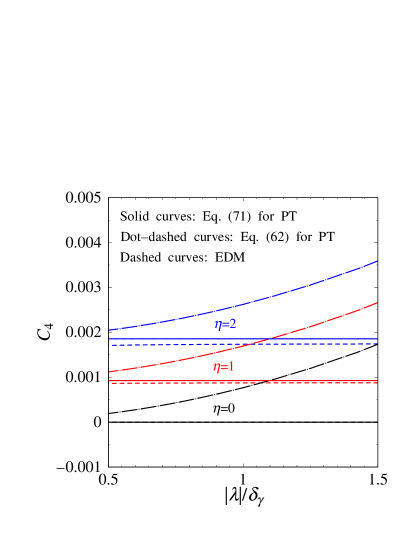
Figure 6: (Color online) The quantity $|\lambda|/\delta_{\gamma}$ dependence of $C_{4}$ for the systems with the crystal field of tetragonal symmetry. We here set $H$=1 eV, $\Delta$=0.1 eV, $\lambda$=$-$0.01 eV, $r$=0, $r_{\gamma}$=0.01, $r_{\varepsilon}/r_{\gamma}$=1, and $\eta$=0, 1, and 2. The solid curves represent $C_{4}$ of Eq. (71) for PT. The dot-dashed curves represent $C_{4}$ of Eq. (3.1) for PT. The dashed curves represent $C_{4}$ of Eq. (59) for the EDM.

3.2 Various features of $C_{2}$ and $C_{4}$

We investigate various features of $C_{2}$ and $C_{4}$ for a strong ferromagnet with $H$=1 eV and $\lambda$=$-$0.01 eV. We here use $C_{2}$ of Eq. (3.1) and $C_{4}$ of Eq. (71) for PT and $C_{2}$ of Eq. (58) and $C_{4}$ of Eq. (59) for the EDM, where $|\lambda|/\delta_{\varepsilon}$=$|\lambda|/\delta_{\gamma}$=1/2 is set for $C_{2}$ and $C_{4}$ for the EDM. We also utilize Eqs. (69) and (70). As a particularly important result, we find that $C_{4}$ appears under the crystal field of tetragonal symmetry, whereas it vanishes under the crystal field of cubic symmetry.[44]

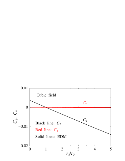
Figure 7: (Color online) The quantity $r_{\varepsilon}/r_{\gamma}$ dependences of $C_{2}$ and $C_{4}$ for the system with the crystal field of cubic symmetry. We here set $H$=1 eV, $\Delta$=0.1 eV, $\lambda$=$-$0.01 eV, $\delta_{\varepsilon}$=$\delta_{\gamma}$=0, $r$=0, $r_{\gamma}$=0.01, and $\eta$=0. The solid lines represent $C_{2}$ of Eq. (58) and $C_{4}$ of Eq. (59) for the EDM.

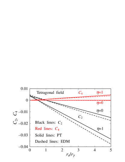
Figure 8: (Color online) The quantity $r_{\varepsilon}/r_{\gamma}$ dependences of $C_{2}$ and $C_{4}$ for the system with the crystal field of tetragonal symmetry. We here set $H$=1 eV, $\Delta$=0.1 eV, $\lambda$=$-$0.01 eV, $r$=0, $r_{\gamma}$=0.01, and $\eta$=0 and 1. The solid lines represent $C_{2}$ of Eq. (3.1) and $C_{4}$ of Eq. (71) for PT. The dashed lines represent $C_{2}$ of Eq. (58) and $C_{4}$ of Eq. (59) for the EDM, where $|\lambda|/\delta_{\varepsilon}$=$|\lambda|/\delta_{\gamma}$=1/2.

Using the EDM, we obtain the $r_{\varepsilon}/r_{\gamma}$ dependences of $C_{2}$ and $C_{4}$ for a system with the crystal field of cubic symmetry, where $\Delta$=0.1 eV, $\delta_{\varepsilon}$=$\delta_{\gamma}$=0, $r$=0, $r_{\gamma}$=0.01, and $\eta$=0 (see Fig. 7). We find that $C_{2}$ can be expressed as a linear function of $r_{\varepsilon}/r_{\gamma}$. The sign of $C_{2}$ changes in the vicinity of $r_{\varepsilon}/r_{\gamma}$$\sim$1. Furthermore, $C_{4}$ takes a value of almost 0.

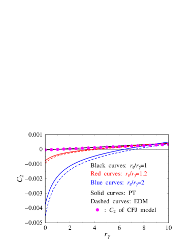
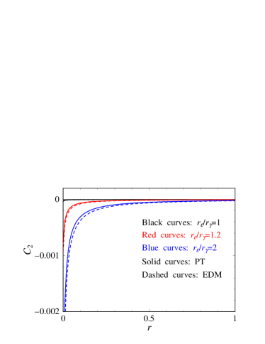
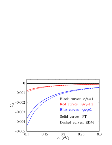
Figure 9: (Color online) The coefficient $C_{2}$ for strong ferromagnets with the crystal field of tetragonal symmetry. We here set $H$=1 eV, $\lambda$=$-$0.01 eV, $r_{\varepsilon}/r_{\gamma}$=1, 1.2, and 2, and $\eta$=0. Upper panel: The quantity $r_{\gamma}$ dependence of $C_{2}$ for the systems with $\Delta$=0.1 eV and $r$=0. Middle panel: The quantity $r$ dependence of $C_{2}$ for the systems with $\Delta$=0.1 eV and $r_{\gamma}$=0.01. Lower panel: The energy $\Delta$ dependence of $C_{2}$ for the systems with $r$=0 and $r_{\gamma}$=0.01. The solid curves represent $C_{2}$ of Eq. (3.1) for PT. The dashed curves represent $C_{2}$ of Eq. (58) for the EDM, where $|\lambda|/\delta_{\varepsilon}$=$|\lambda|/\delta_{\gamma}$=1/2. The dots represent $C_{2}$ of the CFJ model.[2] Note that $C_{4}$ is not shown because $C_{4}$ for PT is 0 and $C_{4}$ for the EDM is much smaller than $|C_{2}|$.

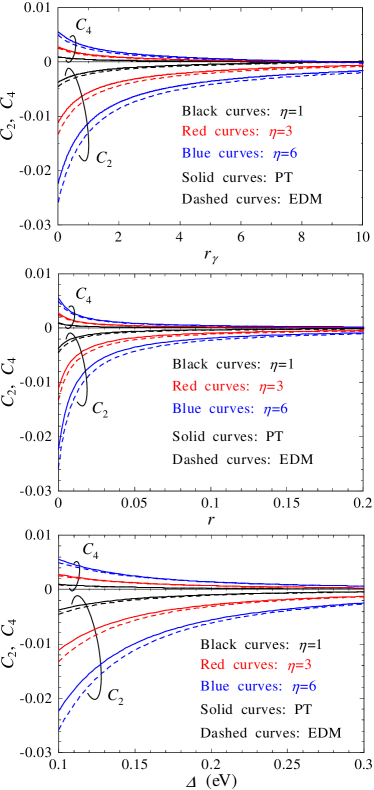
Figure 10: (Color online) The coefficients $C_{2}$ and $C_{4}$ for strong ferromagnets with the crystal field of tetragonal symmetry. We here set $H$=1 eV, $\lambda$=$-$0.01 eV, $r_{\varepsilon}/r_{\gamma}$=1, and $\eta$=1, 3, and 6. Upper panel: The quantity $r_{\gamma}$ dependences of $C_{2}$ and $C_{4}$ for the systems with $\Delta$=0.1 eV and $r$=0. Middle panel: The quantity $r$ dependences of $C_{2}$ and $C_{4}$ for the systems with $\Delta$=0.1 eV and $r_{\gamma}$=0.01. Lower panel: The energy $\Delta$ dependences of $C_{2}$ and $C_{4}$ for the systems with $r$=0 and $r_{\gamma}$=0.01. The solid curves show $C_{2}$ of Eq. (3.1) and $C_{4}$ of Eq. (71) for PT. The dashed curves represent $C_{2}$ of Eq. (58) and $C_{4}$ of Eq. (59) for the EDM, where $|\lambda|/\delta_{\gamma}$=1/2 and $|\lambda|/\delta_{\varepsilon}$=1/2.

Figure 8 shows the $r_{\varepsilon}/r_{\gamma}$ or $\eta$ dependences of $C_{2}$ and $C_{4}$ for a system with the crystal field of tetragonal symmetry, where $\Delta$=0.1 eV, $r$=0, and $\eta$=0 and 1. From the results of PT, we find $C_{2}$$\sim$0 for the system with $r_{\varepsilon 1}/r_{\gamma}$=$r_{\varepsilon}(1+\eta)/r_{\gamma}$=1 and $C_{2}$$\neq$0 for that with $r_{\varepsilon 1}/r_{\gamma}$=$r_{\varepsilon}(1+\eta)/r_{\gamma}$$\neq$1. This feature mainly reflects Eq. (72). We also obtain $C_{4}$=0 for the system with $\eta$=0 and $C_{4}$$\neq$0 for that with $\eta$$\neq$0 because of $C_{4}\propto r_{\varepsilon 1}-r_{\varepsilon 2}$ $(=r_{\varepsilon}\eta)$. The coefficients $C_{2}$ and $C_{4}$ obtained by PT qualitatively agree well with those obtained by the EDM.

In Fig. 9, we show $C_{2}$ for systems with the crystal field of tetragonal symmetry, where $r_{\varepsilon}/r_{\gamma}$=1, 1.2, and 2 and $\eta$=0. Here, $C_{4}$ for PT takes a value of 0 because of $\eta$=0, and $|C_{4}|$ for the EDM is much smaller than $|C_{2}|$. The upper panel shows the $r_{\gamma}$ dependence of $C_{2}$ for systems with $\Delta$=0.1 eV and $r$=0. The middle panel shows the $r$ dependence of $C_{2}$ for systems with $\Delta$=0.1 eV and $r_{\gamma}$=0.01. The lower panel shows the $\Delta$ dependence of $C_{2}$ for systems with $r$=0 and $r_{\gamma}$=0.01. In the upper panel, when $r_{\varepsilon}/r_{\gamma}$=1, $C_{2}$ for PT is close to that for the CFJ model, i.e., $C_{2}$=$(1/2)\Delta\rho(0)/\rho$=$(3/8)(\lambda/H)^{2}(\alpha-1)$, with $\alpha$=$r_{\varepsilon}$=$r_{\gamma}$ (see Appendix E.2). In the middle and lower panels, $C_{2}$ for PT takes a value of almost 0 in the case of $r_{\varepsilon}/r_{\gamma}$=1. The sign of $C_{2}$ for PT is negative in the case of $r_{\varepsilon}/r_{\gamma}$=1.2 or 2. In addition, $|C_{2}|$ for PT increases with decreasing $r$ or $\Delta$ and with increasing $r_{\varepsilon}/r_{\gamma}$. These features mainly reflect Eq. (72). In all panels, $C_{2}$ for PT qualitatively agrees well with that for the EDM.

Figure 10 shows $C_{2}$ and $C_{4}$ for systems with the crystal field of tetragonal symmetry, where $r_{\varepsilon}/r_{\gamma}$=1 and $\eta$=1, 3, and 6. The upper panel shows the $r_{\gamma}$ dependences of $C_{2}$ and $C_{4}$ for systems with $\Delta$=0.1 eV and $r$=0. The middle panel shows the $r$ dependences of $C_{2}$ and $C_{4}$ for systems with $\Delta$=0.1 eV and $r_{\gamma}$=0.01. The lower panel shows the $\Delta$ dependences of $C_{2}$ and $C_{4}$ for systems with $r$=0 and $r_{\gamma}$=0.01. In all panels, the sign of $C_{2}$ for PT is negative, while that of $C_{4}$ for PT is positive. In addition, $|C_{2}|$ and $C_{4}$ for PT increase with decreasing $r_{\gamma}$, $r$, or $\Delta$ and with increasing $\eta$. Such features are mainly due to Eqs. (72) and (73). The coefficients $C_{2}$ and $C_{4}$ for PT qualitatively agree well with those for the EDM.

4 Simple Analysis of $C_{2}$ and $C_{4}$ for Fe₄N

Utilizing the above results, we perform a simple analysis of the experimental results[22] for the $T$ dependences of $C_{2}$ and $C_{4}$ for an Fe₄N[45, 46, 47] film on a MgO(001) substrate, where $I$ flows along Fe₄N [100]. The experimental results clearly show the difference in the behaviors between the low-temperature range of 4 K $\leq T\leq 35$ K and the high-temperature range of 35 K $<T\leq$ 300 K (see circles in Fig. 11). Here, we regard Fe₄N as a strong ferromagnet with $D_{i,+}^{(d)}$$\sim$0.[19] In addition, we mainly focus on the effect of the PDOSs of the $d\varepsilon$ states on $C_{4}$. Note that we do not take into account the realistic crystal structure of Fe₄N (i.e., a perovskite-type structure[45]) for simplicity.[48]

From Eqs. (72) and (73), we first obtain simple expressions for $C_{2}$ and $C_{4}$ for Fe₄N. By taking into account the relation for Fe₄N, i.e., $r\ll 1$ and $r_{\gamma}\ll 1$, [19] $C_{2}$ and $C_{4}$ are given by

$$C_{2}=\frac{3}{8}\left(\frac{\lambda}{\Delta}\right)^{2}\frac{r_{\gamma}-r_{\varepsilon 1}}{r+r_{\gamma}}=\frac{\kappa(1-R_{\varepsilon 1})}{1+R}=\frac{\kappa(1-R_{\varepsilon 2}-\Delta R_{\varepsilon})}{1+R},$$ (74)

$$C_{4}=\frac{3}{32}\left(\frac{\lambda}{\Delta}\right)^{2}\frac{r_{\varepsilon 1}-r_{\varepsilon 2}}{r+r_{\gamma}}=\frac{\displaystyle{\frac{\kappa}{4}}(R_{\varepsilon 1}-R_{\varepsilon 2})}{1+R}=\frac{\displaystyle{\frac{\kappa}{4}\Delta R_{\varepsilon}}}{1+R},$$ (75)

where

$$\kappa=\frac{3}{8}\left(\frac{\lambda}{\Delta}\right)^{2},R_{\varepsilon 1}=\frac{r_{\varepsilon 1}}{r_{\gamma}},~{}R_{\varepsilon 2}=\frac{r_{\varepsilon 2}}{r_{\gamma}},~{}\Delta R_{\varepsilon}=R_{\varepsilon 1}-R_{\varepsilon 2},$$

$$R=\frac{r}{r_{\gamma}}=\frac{\rho_{s,-}/\rho_{s,+}}{\rho_{s\to d_{\gamma},-}/\rho_{s,+}}=\frac{\rho_{s,-}}{\rho_{s\to d_{\gamma},-}},$$ (76)

with $\rho_{s\to d_{\gamma},-}$=$\rho_{s\to d_{x^{2}-y^{2}},-}$=$\rho_{s\to d_{3z^{2}-r^{2}},-}$. Here, $\Delta R_{\varepsilon}$ is proportional to $D_{\varepsilon 1,-}^{(d)}-D_{\varepsilon 2,-}^{(d)}$, which is the difference in the PDOSs at $E_{\mbox{\tiny F}}$ among the d$\varepsilon$ states.

We next determine parameter sets for $\lambda$, $\Delta$, $R$, $R_{\varepsilon 1}$, $R_{\varepsilon 2}$, and $\Delta R_{\varepsilon}$ that can reproduce the experimental result for the $T$ dependences of $C_{2}$ and $C_{4}$. The quantity $\lambda$ is set to $\lambda$=$-$0.013 eV for Fe.[36] The quantity $\Delta$ is assumed to be $\Delta$=0.1 eV.[37] Here, the $T$ dependence of $\Delta$ is considered to be negligibly small, because the decrease in the lattice constant due to a decrease in $T$ is less than 0.5%,[22] where $\Delta$ of 0.1 eV is due to the Coulomb interaction between a magnetic ion and the surrounding ions. We accordingly adopt the $T$ dependences of $R$, $R_{\varepsilon 1}$, $R_{\varepsilon 2}$, and $\Delta R_{\varepsilon}$. The $T$ dependence of $R$ ($R_{\varepsilon 1}$, $R_{\varepsilon 2}$, and $\Delta R_{\varepsilon}$) is shown in the middle (lower) panel of Fig. 11. Details of the parameter sets are given below.

We express $R$ of Eq. (76) as

$$R=\frac{\rho_{s,-}}{\rho_{s\to d_{\gamma},-}}=\frac{\rho_{s,-}^{\rm imp}+\rho_{s,-}^{\rm ph}}{\rho_{s\to d_{\gamma},-}^{\rm imp}},$$ (77)

where $\rho_{s,-}$ and $\rho_{s\to d_{\gamma},-}$ are assumed to be $\rho_{s,-}$=$\rho_{s,-}^{\rm imp}+\rho_{s,-}^{\rm ph}$ and $\rho_{s\to d_{\gamma},-}$=$\rho_{s\to d_{\gamma},-}^{\rm imp}$ (see Sec. 2.5). The quantity $\rho_{s,-}^{\rm imp}$ is the $s$–$s$ resistivity due to impurities and $\rho_{s\to d_{\gamma},-}^{\rm imp}$ is the $s$–$d$ resistivity due to impurities, where $d_{\gamma},-$ represents the $d\gamma$ states of the down spin. Here, $\rho_{s,-}^{\rm imp}/\rho_{s\to d_{\gamma},-}^{\rm imp}$ is set so that

$$\frac{\rho_{s,-}^{\rm imp}}{\rho_{s\to d_{\gamma},-}^{\rm imp}}\ll 1,$$ (78)

by considering that $\rho_{s\to d_{\gamma},-}^{\rm imp}$ ($\rho_{s,-}^{\rm imp}$) satisfies the relation $\rho_{s\to d_{\gamma},-}^{\rm imp}\propto D_{\gamma,-}^{(d)}$ ($\rho_{s,-}^{\rm imp}\propto D_{-}^{(s)}$[49]) and also Fe₄N satisfies $D_{\gamma,-}^{(d)}\gg D_{-}^{(s)}$. On the other hand, $\rho_{s,-}^{\rm ph}$ is the $s$–$s$ resistivity due to the phonons. This $\rho_{s,-}^{\rm ph}$ depends on $T$ through the influence of the number of phonons, which depends on $T$.

The parameter sets in the high- and low-temperature ranges are noted below.

1. In the high-temperature range of $T>$ 35 K, we have

   $$R=\Theta T,$$ (79)

   $$\Delta R_{\varepsilon}=0,$$ (80)

   $$R_{\varepsilon 2}=R_{\varepsilon 1}=1-\frac{C_{2}^{(T^{*})}}{\kappa}(1+R^{*}),$$ (81)

   with $\Theta$=0.0270, $T^{*}$=35 K, $R^{*}$=$\Theta T^{*}$, and $C_{2}^{(T^{*})}$=$-$0.0126, where $C_{2}^{(T^{*})}$ is the experimental value of $C_{2}$ at $T$=$T^{*}$.[22]

   The procedure for determining this parameter set is as follows: First, $C_{4}$ is experimentally observed to be almost 0. Since $C_{4}\propto\Delta R_{\varepsilon}$ [see Eq. (75)], we assume $\Delta R_{\varepsilon}$=0 (or $R_{\varepsilon 1}$=$R_{\varepsilon 2}$); that is, the PDOSs of the $d\varepsilon$ states at $E_{\mbox{\tiny F}}$ take the same value. From the viewpoint of the crystal structure of Fe₄N, this assumption may imply that the crystal exhibits cubic symmetry.[48] Next, since $|C_{2}|$ gradually decreases with increasing $T$, we straightforwardly take into consideration the $T$ dependence of $R$ of Eq. (77), where $R$ is included in the denominator of $C_{2}$ of Eq. (74). The denominator $1+R$ is expressed as

   $$1+R\approx 1+\frac{\rho_{s,-}^{\rm ph}}{\rho_{s\to d_{\gamma},-}^{\rm imp}},$$ (82)

   by using Eqs. (77) and (78). Here, $\rho_{s,-}^{\rm ph}$ is assumed to be proportional to $T$ on the basis of the experimental result for the $T$ dependence of the total resistivity.[50] Thereby, $R$ ($\approx\rho_{s,-}^{\rm ph}/\rho_{s\to d_{\gamma},-}^{\rm imp}$) is given by

   $$R=\theta T,$$ (83)

   where $\theta$ is a constant number. On the other hand, $R_{\varepsilon 2}$ is determined so that Eq. (74) satisfies the condition $(T,C_{2})$=$(T^{*},C_{2}^{(T^{*})})$. Namely, $R_{\varepsilon 2}$ is expressed as $R_{\varepsilon 2}$=$1-(C_{2}^{(T^{*})}/\kappa)(1+\theta T^{*})$. Substituting this $R_{\varepsilon 2}$ and $\Delta R_{\varepsilon}$=0 into Eq. (74), we obtain

   $$C_{2}=\frac{C_{2}^{(T^{*})}(1+\theta T^{*})}{1+\theta T}.$$ (84)

   From the least-square fitting of Eq. (84) to the experimental result for $C_{2}$, we determine $\theta$ to be $\Theta$ (=0.0270),[51] where the fitting is done for $T$=35$-$150 K by paying attention to the relatively low temperature side. Using $\Theta$=0.0270, we can also evaluate $R_{\varepsilon 2}$ of Eq. (81).

2. In the low-temperature range of $T\leq$ 35 K, we have

   $$R=\Theta T,$$ (85)

   $$\Delta R_{\varepsilon}=\frac{T-T^{*}}{T_{l}-T^{*}}\left(\frac{1+R}{\kappa/4}C_{4}^{(T_{l})}\right),$$ (86)

   $$R_{\varepsilon 2}=\frac{R_{\varepsilon 2}^{*}-R_{\varepsilon 2}^{(l)}}{T^{*}-T_{l}}T+\frac{R_{\varepsilon 2}^{(l)}T^{*}-R_{\varepsilon 2}^{*}T_{l}}{T^{*}-T_{l}},$$ (87)

   $$R_{\varepsilon 1}=R_{\varepsilon 2}+\Delta R_{\varepsilon},$$ (88)

   with $T_{l}$=4 K, $R_{\varepsilon 2}^{*}$=$1-(1+R^{*})C_{2}^{(T^{*})}/\kappa$, $R_{\varepsilon 2}^{(l)}$=$1-(1+R_{l})(C_{2}^{(T_{l})}+4C_{4}^{(T_{l})})/\kappa$, $R_{l}$=$\Theta T_{l}$, $C_{2}^{(T_{l})}$=$-$0.0343, and $C_{4}^{(T_{l})}$=0.00556, where $C_{2}^{(T_{l})}$ ($C_{4}^{(T_{l})}$) is the experimental value of $C_{2}$ at $T$=$T_{l}$ ($C_{4}$ at $T$=$T_{l}$).[22]

   The procedure for determining this parameter set is as follows: We first adopt $R$=$\Theta T$, which is the same as Eq. (79) in the high-temperature range, on the basis of the expeimental result of the $T$ dependence of the total resistivity.[50] Second, since $C_{4}$ was experimentally observed to be a linear function of $T$, we assume $C_{4}$ to be $C_{4}$=$pT+q$, where $p$ and $q$ are constants. The constants $p$ and $q$ are determined so that Eq. (75) satisfies the condition $(T,C_{4})$=$(T_{l},C_{4}^{(T_{l})})$, $(T^{*},0)$. As a result, $C_{4}$ is expressed as $C_{4}$=$(T-T^{*})C_{4}^{(T_{l})}/(T_{l}-T^{*})$. From this $C_{4}$ and Eq. (75), we obtain $\Delta R_{\epsilon}$ of Eq. (86). The obtained $\Delta R_{\epsilon}$ may indicate the following two properties: One is that the crystal has tetragonal symmetry, which generates $\Delta R_{\varepsilon}$$\neq$0 due to the difference of the PDOS at $E_{\mbox{\tiny F}}$ among the d$\varepsilon$ states. The other is that the tetragonal distortion increases with decreasing $T$. Third, $R_{\varepsilon 2}$ is assumed to be $R_{\varepsilon 2}$=$p^{\prime}T+q^{\prime}$ as a simple form, where $p^{\prime}$ and $q^{\prime}$ are constants. The constants $p^{\prime}$ and $q^{\prime}$ are determined so that Eq. (74) satisfies the condition $(T,C_{2})$=$(T_{l},C_{2}^{(T_{l})})$, $(T^{*},C_{2}^{(T^{*})})$.

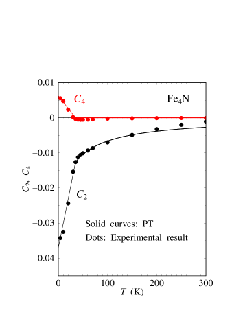
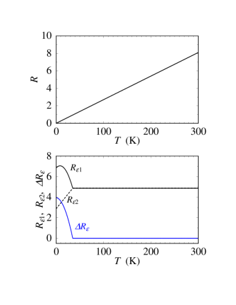
Figure 11: (Color online) Upper panel: The $T$ dependences of $C_{2}$ and $C_{4}$ for Fe₄N. The solid curves represent Eqs. (74) and (75) for PT. The dots represent the experimental values in the temperature range from 4 to 300 K for the case of ${\mbox{\boldmath$I$}}//$Fe₄N [100].[22] Middle panel: The $T$ dependence of $R$ in Eq. (4). The expression for $R$ is given by Eqs. (79) and (85). Lower panel: The $T$ dependences of $R_{\varepsilon 1}$, $R_{\varepsilon 2}$, and $\Delta R_{\varepsilon}$ in Eq. (4). The expressions for $R_{\varepsilon 1}$, $R_{\varepsilon 2}$, and $\Delta R_{\varepsilon}$ are given by Eqs. (81) and (88), (81) and (87), and (80) and (86), respectively. The black solid curve (black dashed curve) represents $R_{\varepsilon 1}$ ($R_{\varepsilon 2}$). The blue solid curve represents $\Delta R_{\varepsilon}$.

Substituting the above-mentioned $\lambda$ and $\Delta$, Eqs. (79)$-$(81), and Eqs. (85)$-$(87) into Eqs. (74) and (75), we obtain $C_{2}$ and $C_{4}$ for Fe₄N, where $C_{4}$ in the low-temperature range was described above. In the upper panel of Fig. 11, we show the $T$ dependences of $C_{2}$ and $C_{4}$. We find that $C_{2}$ and $C_{4}$ for PT successfully reproduce the experimental results. In particular, the experimental results in the range 4 K $\leq T\leq$ 35 K, in which the change of $|C_{2}|$ is about four times as large as that of $|C_{4}|$, can be explained by the ratio of the coefficients of $\Delta R_{\varepsilon}$ between Eqs. (74) and (75).

Finally, we comment on the above-mentioned $T$ dependence of $\Delta R_{\varepsilon}$, i.e., the difference in the PDOSs at $E_{\mbox{\tiny F}}$ among the d$\varepsilon$ states. The $T$ dependence of $\Delta R_{\varepsilon}$ has been assumed to arise from the increase of the tetragonal distortion due to a decrease in $T$. The tetragonal distortion may originate from the anisotropic thermal compression of the lattice. This compression is considered to be due to the adhesion between the Fe₄N film and the MgO substrate. We expect that such an assumption will be verified experimentally in the future.

5 Conclusions

We theoretically studied the twofold and fourfold symmetric AMR effects of ferromagnets. In particular, we obtained the coefficients of the twofold symmetric term ($\cos 2\phi$ term) and the fourfold symmetric term ($\cos 4\phi$ term) in the AMR ratio, denoted as $C_{2}$ and $C_{4}$, respectively. We used the two-current model for the system consisting of the conduction state and localized d states. The localized d states were obtained from the Hamiltonian with the spin–orbit interaction, the exchange field, and the crystal field. Details are given as follows:

1. We performed the numerical calculation of $C_{2}$ and $C_{4}$ for a strong ferromagnet using d states, which were obtained by applying the EDM to the Hamiltonian. The result revealed that $C_{4}$ appears under the crystal field of tetragonal symmetry, whereas it vanishes under the crystal field of cubic symmetry.

2. We derived general expressions for the resistivity, $C_{2}$, and $C_{4}$ for ferromagnets with the tetragonal field using the d states, which were obtained by applying first- and second-order PT to the Hamiltonian. From the expressions, we obtained expressions for $C_{2}$ and $C_{4}$ for the strong ferromagnet with the tetragonal field. The result showed that $C_{2}\cos 2\phi$ is related to the real part of the probability amplitudes of the specific hybridized states $|3z^{2}-r^{2},\chi_{\sigma}(\phi)\rangle$ and $|x^{2}-y^{2},\chi_{\sigma}(\phi)\rangle$ and $C_{4}\cos 4\phi$ is related to the probabilities of $|3z^{2}-r^{2},\chi_{\sigma}(\phi)\rangle$ and $|x^{2}-y^{2},\chi_{\sigma}(\phi)\rangle$. In addition, we investigated various features of $C_{2}$ and $C_{4}$ obtained by PT and found that they qualitatively agreed well with those obtained by the EDM.

3. We analyzed the experimental results of the $T$ dependences of $C_{2}$ and $C_{4}$ for an Fe₄N film on a MgO substrate using the dominant terms in $C_{2}$ and $C_{4}$ obtained by PT. The dominant term in $C_{2}$ was proportional to the difference in the PDOSs at $E_{\mbox{\tiny F}}$ between the $d\varepsilon$ and $d\gamma$ states, and that in $C_{4}$ was proportional to the difference in the PDOSs at $E_{\mbox{\tiny F}}$ among the $d\varepsilon$ states. The experimental results in the high-temperature range (35 K $<T\leq$ 300 K) were well reproduced by taking into account the $T$ dependence of the $s$–$s$ resistivity and by assuming that the PDOSs of the $d\varepsilon$ states at $E_{\mbox{\tiny F}}$ took the same value. This assumption might imply that the crystal structure of Fe₄N exhibits cubic symmetry. Also, the experimental results in the low-temperature range (4 K $\leq T\leq$ 35 K) were successfully reproduced by assuming that the difference in the PDOSs at $E_{\mbox{\tiny F}}$ among the $d\varepsilon$ states increased with decreasing $T$. This assumption suggested that the tetragonal distortion increases with decreasing $T$. Here, the tetragonal distortion was considered to originate from the anisotropic thermal compression of the lattice due to the adhesion between the MgO substrate and Fe₄N film.

Appendix A Matrix Representation of ${\cal H}$

We construct the matrix of ${\cal H}$ of Eq. (4) as shown in Table 2.

In the construction, we perform, for example, the following operations:

$$\lambda L_{y}S_{y}|xz,\chi_{-}(\phi)\rangle = \lambda L_{y}|xz\rangle S_{y}|\chi_{-}(\phi)\rangle$$

$$= i\lambda(-|x^{2}-y^{2}\rangle+\sqrt{3}|3z^{2}-r^{2}\rangle)\frac{1}{2}(i\cos\phi|\chi_{+}(\phi)\rangle+\sin\phi|\chi_{-}(\phi)\rangle),$$

$$\lambda L_{x}S_{x}|yz,\chi_{-}(\phi)\rangle = \lambda L_{x}|yz\rangle S_{x}|\chi_{-}(\phi)\rangle$$

$$= i\lambda(|x^{2}-y^{2}\rangle+\sqrt{3}|3z^{2}-r^{2}\rangle)\frac{1}{2}(i\sin\phi|\chi_{+}(\phi)\rangle-\cos\phi|\chi_{-}(\phi)\rangle).$$

Equations (A) and (A) play an important role in $C_{2}$ and $C_{4}$, as described when we discuss the $\phi$ dependence of the wave functions (see Sec. 2.2).

Table 2: Matrix representation of ${\cal H}$ of Eq. (4) in the basis set $|xy,\chi_{+}(\phi)\rangle$, $|yz,\chi_{+}(\phi)\rangle$, $|xz,\chi_{+}(\phi)\rangle$, $|xy,\chi_{-}(\phi)\rangle$, $|yz,\chi_{-}(\phi)\rangle$, $|xz,\chi_{-}(\phi)\rangle$, $|x^{2}-y^{2},\chi_{+}(\phi)\rangle$, $|3z^{2}-r^{2},\chi_{+}(\phi)\rangle$, $|x^{2}-y^{2},\chi_{-}(\phi)\rangle$, and $|3z^{2}-r^{2},\chi_{-}(\phi)\rangle$. In this table, $(\phi)$ in $\chi_{\sigma}(\phi)$ is omitted due to limited space.

	$|xy,\chi_{+}\rangle$	$|yz,\chi_{+}\rangle$	$|xz,\chi_{+}\rangle$	$|xy,\chi_{-}\rangle$	$|yz,\chi_{-}\rangle$	$|xz,\chi_{-}\rangle$	$|x^{2}-y^{2}$, $\chi_{+}\rangle$	$|3z^{2}-r^{2}$, $\chi_{+}\rangle$	$|x^{2}-y^{2}$, $\chi_{-}\rangle$	$|3z^{2}-r^{2}$, $\chi_{-}\rangle$
$\langle xy,\chi_{+}|$	$-\frac{H}{2}$	$i\frac{\lambda}{2}\sin\phi$	$-i\frac{\lambda}{2}\cos\phi$	0	$\frac{\lambda}{2}\cos\phi$	$\frac{\lambda}{2}\sin\phi$	0	0	$-i\lambda$	0
$\langle yz,\chi_{+}|$	$-i\frac{\lambda}{2}\sin\phi$	$-\frac{H}{2}+\delta_{\varepsilon}$	0	$-\frac{\lambda}{2}\cos\phi$	0	$-i\frac{\lambda}{2}$	$-i\frac{\lambda}{2}\cos\phi$	$-i\frac{\sqrt{3}\lambda}{2}\cos\phi$	$\frac{\lambda}{2}\sin\phi$	$\frac{\sqrt{3}\lambda}{2}\sin\phi$
$\langle xz,\chi_{+}|$	$i\frac{\lambda}{2}\cos\phi$	0	$-\frac{H}{2}+\delta_{\varepsilon}$	$-\frac{\lambda}{2}\sin\phi$	$i\frac{\lambda}{2}$	0	$-i\frac{\lambda}{2}\sin\phi$	$i\frac{\sqrt{3}\lambda}{2}\sin\phi$	$-\frac{\lambda}{2}\cos\phi$	$\frac{\sqrt{3}\lambda}{2}\cos\phi$
$\langle xy,\chi_{-}|$	0	$-\frac{\lambda}{2}\cos\phi$	$-\frac{\lambda}{2}\sin\phi$	$\frac{H}{2}$	$-i\frac{\lambda}{2}\sin\phi$	$i\frac{\lambda}{2}\cos\phi$	$-i\lambda$	0	0	0
$\langle yz,\chi_{-}|$	$\frac{\lambda}{2}\cos\phi$	0	$-i\frac{\lambda}{2}$	$i\frac{\lambda}{2}\sin\phi$	$\frac{H}{2}+\delta_{\varepsilon}$	0	$-\frac{\lambda}{2}\sin\phi$	$-\frac{\sqrt{3}\lambda}{2}\sin\phi$	$i\frac{\lambda}{2}\cos\phi$	$i\frac{\sqrt{3}\lambda}{2}\cos\phi$
$\langle xz,\chi_{-}|$	$\frac{\lambda}{2}\sin\phi$	$i\frac{\lambda}{2}$	0	$-i\frac{\lambda}{2}\cos\phi$	0	$\frac{H}{2}+\delta_{\varepsilon}$	$\frac{\lambda}{2}\cos\phi$	$-\frac{\sqrt{3}\lambda}{2}\cos\phi$	$i\frac{\lambda}{2}\sin\phi$	$-i\frac{\sqrt{3}\lambda}{2}\sin\phi$
$\langle x^{2}-y^{2}$, $\chi_{+}|$	0	$i\frac{\lambda}{2}\cos\phi$	$i\frac{\lambda}{2}\sin\phi$	$i\lambda$	$-\frac{\lambda}{2}\sin\phi$	$\frac{\lambda}{2}\cos\phi$	$-\frac{H}{2}+\Delta$	0	0	0
$\langle 3z^{2}-r^{2}$, $\chi_{+}|$	0	$i\frac{\sqrt{3}\lambda}{2}\cos\phi$	$-i\frac{\sqrt{3}\lambda}{2}\sin\phi$	0	$-\frac{\sqrt{3}\lambda}{2}\sin\phi$	$-\frac{\sqrt{3}\lambda}{2}\cos\phi$	0	$-\frac{H}{2}+\Delta+\delta_{\gamma}$	0	0
$\langle x^{2}-y^{2}$, $\chi_{-}|$	$i\lambda$	$\frac{\lambda}{2}\sin\phi$	$-\frac{\lambda}{2}\cos\phi$	0	$-i\frac{\lambda}{2}\cos\phi$	$-i\frac{\lambda}{2}\sin\phi$	0	0	$\frac{H}{2}+\Delta$	0
$\langle 3z^{2}-r^{2}$, $\chi_{-}|$	0	$\frac{\sqrt{3}\lambda}{2}\sin\phi$	$\frac{\sqrt{3}\lambda}{2}\cos\phi$	0	$-i\frac{\sqrt{3}\lambda}{2}\cos\phi$	$i\frac{\sqrt{3}\lambda}{2}\sin\phi$	0	0	0	$\frac{H}{2}+\Delta+\delta_{\gamma}$

Appendix B Zero-Order States

Performing the unitary transformation for $V$ of Eq. (6), we obtain the zero-order states.[38]

Table 3 shows the matrix representation of $V$ in the subspace with the basis set $|xy,\chi_{\sigma}(\phi)\rangle$, $|yz,\chi_{\sigma}(\phi)\rangle$, and $|xz,\chi_{\sigma}(\phi)\rangle$, with $\sigma$=$+$ or $-$. The eigenvalues of $V$ are obtained as $\xi_{+}$, $\delta_{\varepsilon}$, and $\xi_{-}$, with

$$\xi_{\pm}=\frac{\delta_{\varepsilon}\pm\sqrt{\delta_{\varepsilon}^{2}+\lambda^{2}}}{2}.$$ (91)

In the case of $\sigma$=$+$, the eigenstates for $\xi_{+}$, $\delta_{\varepsilon}$, and $\xi_{-}$ are respectively given by $|\xi_{+},\chi_{+}(\phi)\rangle$ of Eq. (2.2), $|\delta_{\varepsilon},\chi_{+}(\phi)\rangle$ of Eq. (16), and $|\xi_{-},\chi_{-}(\phi)\rangle$ of Eq. (2.2). In the case of $\sigma$=$-$, the eigenstates for $\xi_{+}$, $\delta_{\varepsilon}$, and $\xi_{-}$ are $|\xi_{+},\chi_{-}(\phi)\rangle$ of Eq. (2.2), $|\delta_{\varepsilon},\chi_{-}(\phi)\rangle$ of Eq. (19), and $|\xi_{-},\chi_{-}(\phi)\rangle$ of Eq. (2.2), respectively. These states correspond to the zero-order states in PT.

Table 3: Matrix representation of $V$ of Eq. (6) in the subspace with the basis set $|xy,\chi_{\pm}(\phi)\rangle$, $|yz,\chi_{\pm}(\phi)\rangle$, and $|xz,\chi_{\pm}(\phi)\rangle$.

	$|xy,\chi_{\pm}(\phi)\rangle$	$|yz,\chi_{\pm}(\phi)\rangle$	$|xz,\chi_{\pm}(\phi)\rangle$
$\langle xy,\chi_{\pm}(\phi)|$	0	$\pm i\frac{\lambda}{2}\sin\phi$	$\mp i\frac{\lambda}{2}\cos\phi$
$\langle yz,\chi_{\pm}(\phi)|$	$\mp i\frac{\lambda}{2}\sin\phi$	$\delta_{\varepsilon}$	0
$\langle xz,\chi_{\pm}(\phi)|$	$\pm i\frac{\lambda}{2}\cos\phi$	0	$\delta_{\varepsilon}$

Appendix C Overlap Integral of $s$–$d$ Scattering Rate

We briefly discuss $|(i,\chi_{\varsigma}(\phi)|e^{ik_{\sigma}x},\chi_{\sigma}(\phi)\rangle|^{2}$ in Eq. (38), where $|i,\chi_{\varsigma}(\phi))$ is represented by a linear combination of $|xy,\chi_{\sigma}(\phi)\rangle$, $|yz,\chi_{\sigma}(\phi)\rangle$, $|xz,\chi_{\sigma}(\phi)\rangle$, $|x^{2}-y^{2},\chi_{\sigma}(\phi)\rangle$, and $|3z^{2}-r^{2},\chi_{\sigma}(\phi)\rangle$.

On the basis of a previous study,[3] we first give the following overlap integral:

$$\langle\mu\nu,\chi_{\sigma^{\prime}}(\phi)|e^{i{\mbox{\boldmath$k$}}_{\sigma}\cdot{\mbox{\boldmath$r$}}},\chi_{\sigma}(\phi)\rangle=\int_{-\infty}^{\infty}\int_{-\infty}^{\infty}\int_{-\infty}^{\infty}f(r)\mu\nu\frac{1}{\sqrt{\Omega}}e^{i{\mbox{\boldmath$k$}}_{\sigma}\cdot{\mbox{\boldmath$r$}}}dxdydz\delta_{\sigma,\sigma^{\prime}}$$ (92)

$$\hskip 56.9055pt=\frac{32\pi\Gamma\zeta}{\sqrt{\Omega}(k_{\sigma}^{2}+\zeta^{2})^{3}}\left(\delta_{\mu,\nu}-\frac{6k_{\mu,\sigma}k_{\nu,\sigma}}{k_{\sigma}^{2}+\zeta^{2}}\right)\delta_{\sigma,\sigma^{\prime}}.$$

Here, we have $|e^{i{\mbox{\boldmath$k$}}_{\sigma}\cdot{\mbox{\boldmath$r$}}},\chi_{\sigma}(\phi)\rangle$= $(1/\sqrt{\Omega})e^{i{\mbox{\boldmath$k$}}_{\sigma}\cdot{\mbox{\boldmath$r$}}}\chi_{\sigma}(\phi)$ (see Sec. 2.5), ${\mbox{\boldmath$k$}}_{\sigma}$ =$(k_{x,\sigma},k_{y,\sigma},k_{z,\sigma})$, $k_{\sigma}$=$|{\mbox{\boldmath$k$}}_{\sigma}|$, and $|\mu\nu,\chi_{\sigma^{\prime}}(\phi)\rangle$=$f(r)\mu\nu\chi_{\sigma^{\prime}}$, with $\mu$=$x$, $y$, $z$, $\nu$=$x$, $y$, $z$, $\sigma$=$+$, $-$, and $\sigma^{\prime}$=$+$, $-$, where $f(r)$ is the radial part of the 3d orbital expressed by $f(r)$=$\Gamma e^{-\zeta r}$, and $\Gamma$ and $\zeta$ are constants. The state $|\mu\nu,\chi_{\sigma^{\prime}}(\phi)\rangle$ denotes the $\mu\nu$ orbital with $\sigma^{\prime}$ spin.

Using Eq. (92), we can calculate the overlap integrals for realistic orbitals. In the case of ${\mbox{\boldmath$k$}}_{\sigma}$=$(k_{\sigma},0,0)$, corresponding to ${\mbox{\boldmath$I$}}//x$ (see Sec. 2.5), we have

$$\langle x^{2}-y^{2},\chi_{\sigma^{\prime}}(\phi)|e^{ik_{\sigma}x},\chi_{\sigma}(\phi)\rangle=\frac{1}{2}g_{\sigma}\delta_{\sigma,\sigma^{\prime}},$$ (93)

$$\langle 3z^{2}-r^{2},\chi_{\sigma^{\prime}}(\phi)|e^{ik_{\sigma}x},\chi_{\sigma}(\phi)\rangle=-\frac{1}{2\sqrt{3}}g_{\sigma}\delta_{\sigma,\sigma^{\prime}},$$ (94)

$$\langle xy,\chi_{\sigma^{\prime}}(\phi)|e^{ik_{\sigma}x},\chi_{\sigma}(\phi)\rangle=\langle yz,\chi_{\sigma^{\prime}}(\phi)|e^{ik_{\sigma}x},\chi_{\sigma}(\phi)\rangle=\langle xz,\chi_{\sigma^{\prime}}(\phi)|e^{ik_{\sigma}x},\chi_{\sigma}(\phi)\rangle=0,$$

with

$$g_{\sigma}=-\frac{192\pi\Gamma\zeta k_{\sigma}^{2}}{\sqrt{\Omega}(k_{\sigma}^{2}+\zeta^{2})^{4}}.$$ (96)

Equations (93)$-$(C) mean that only $|3z^{2}-r^{2},\chi_{\sigma}(\phi)\rangle$ and $|x^{2}-y^{2},\chi_{\sigma}(\phi)\rangle$ contribute to the transport of ${\mbox{\boldmath$I$}}//x$.

Next, using Eqs. (93)$-$(96), we obtain $\left|(i,\chi_{\varsigma}(\phi)|e^{ik_{\sigma}x},\chi_{\sigma}(\phi)\rangle\right|^{2}$ in Eq. (38). Here, $|i,\chi_{\varsigma}(\phi))$ is given simply by $|i,\chi_{\varsigma}(\phi))$=$\sum_{j}\sum_{\sigma}a_{j,\sigma}^{i,\varsigma}(\phi)|j,\chi_{\sigma}(\phi)\rangle$, where $a_{j,\sigma}^{i,\varsigma}(\phi)$ is the coefficient of $|j,\chi_{\sigma}(\phi)\rangle$. In the case of $j$=$x^{2}-y^{2}$ or $3z^{2}-r^{2}$, $a_{j,\sigma}^{i,\varsigma}(\phi)$ corresponds to $c_{i,\varsigma}$, $c_{i,\varsigma}w_{j,\sigma}^{i,\varsigma}\cos 2\phi$, or $c_{i,\varsigma}w_{j,\sigma}^{i,\varsigma}\sin 2\phi$, as seen from Eqs. (25)$-$(2.2). As a result, $\left|(i,\chi_{\varsigma}(\phi)|e^{ik_{\sigma}x},\chi_{\sigma}(\phi)\rangle\right|^{2}$ is expressed as

$$\left|(i,\chi_{\varsigma}(\phi)|e^{ik_{\sigma}x},\chi_{\sigma}(\phi)\rangle\right|^{2}=\left|\frac{1}{2}a_{x^{2}-y^{2},\sigma}^{i,\varsigma}(\phi)g_{\sigma}-\frac{1}{2\sqrt{3}}a_{3z^{2}-r^{2},\sigma}^{i,\varsigma}(\phi)g_{\sigma}\right|^{2}.$$ (97)

In addition, $\left|(i,\chi_{\varsigma}(\phi)|e^{ik_{\sigma}x},\chi_{\sigma}(\phi)\rangle\right|^{2}$ leads to the following two types of expressions (see Table 4). Type 1 is written as

$$\left|\ell_{0}+\ell_{\rm c}\cos 2\phi\right|^{2}=|\ell_{0}|^{2}+\frac{1}{2}|\ell_{\rm c}|^{2}+(\ell_{0}^{*}\ell_{\rm c}+\ell_{0}\ell_{\rm c}^{*})\cos 2\phi+\frac{1}{2}|\ell_{\rm c}|^{2}\cos 4\phi,$$ (98)

where $\ell_{0}$ ($\ell_{\rm c}$) is the coefficient of the constant term ($\cos 2\phi$ term). Type 2 is

$$\left|\ell_{\rm s}\sin 2\phi\right|^{2}=\frac{1}{2}|\ell_{\rm s}|^{2}-\frac{1}{2}|\ell_{\rm s}|^{2}\cos 4\phi,$$ (99)

where $\ell_{\rm s}$ is the coefficient of the $\sin 2\phi$ term. Type 1 generates the twofold and fourfold symmetric terms and type 2 generates the fourfold symmetric term.

Table 4: Expressions for $\left|(i,\chi_{\varsigma}(\phi)|e^{ik_{\sigma}x},\chi_{\sigma}(\phi)\rangle\right|^{2}$. Types 1 and 2 are given by Eqs. (98) and (99), respectively. Here, Eqs. (93)$-$(96) are used.

$i$	$\varsigma$	$\sigma$	$\left|(i,\chi_{\varsigma}(\phi)|e^{ik_{\sigma}x},\chi_{\sigma}(\phi)\rangle\right|^{2}$	type
$\xi_{+}$	$+$	$+$	$g_{+}^{2}\left|\frac{1}{2\sqrt{3}}c_{\xi_{+},+}w_{3z^{2}-r^{2},+}^{\xi_{+},+}\sin 2\phi\right|^{2}$	2
$\delta_{\varepsilon}$	$+$	$+$	$g_{+}^{2}\left|c_{\delta_{\varepsilon},+}\left(\frac{1}{2}-\frac{1}{2\sqrt{3}}w_{3z^{2}-r^{2},+}^{\delta_{\varepsilon},+}\cos 2\phi\right)\right|^{2}$	1
$\xi_{-}$	$+$	$+$	$g_{+}^{2}\left|\frac{1}{2\sqrt{3}}c_{\xi_{-},+}w_{3z^{2}-r^{2},+}^{\xi_{-},+}\sin 2\phi\right|^{2}$	2
$x^{2}-y^{2}$	$+$	$+$	$g_{+}^{2}\left|c_{x^{2}-y^{2},+}\left(\frac{1}{2}-\frac{1}{2\sqrt{3}}w_{3z^{2}-r^{2},+}^{x^{2}-y^{2},+}\cos 2\phi\right)\right|^{2}$	1
$3z^{2}-r^{2}$	$+$	$+$	$g_{+}^{2}\left|c_{3z^{2}-r^{2},+}\left(-\frac{1}{2\sqrt{3}}+\frac{1}{2}w_{x^{2}-y^{2},+}^{3z^{2}-r^{2},+}\cos 2\phi\right)\right|^{2}$	1
$\xi_{+}$	$+$	$-$	$g_{-}^{2}\left|c_{\xi_{+},+}\left(\frac{1}{2}-\frac{1}{2\sqrt{3}}w_{3z^{2}-r^{2},-}^{\xi_{+},+}\cos 2\phi\right)\right|^{2}$	1
$\delta_{\varepsilon}$	$+$	$-$	$g_{-}^{2}\left|\frac{1}{2\sqrt{3}}c_{\delta_{\varepsilon},+}w_{3z^{2}-r^{2},-}^{\delta_{\varepsilon},+}\sin 2\phi\right|^{2}$	2
$\xi_{-}$	$+$	$-$	$g_{-}^{2}\left|c_{\xi_{-},+}\left(\frac{1}{2}-\frac{1}{2\sqrt{3}}w_{3z^{2}-r^{2},-}^{\xi_{-},+}\cos 2\phi\right)\right|^{2}$	1
$\xi_{+}$	$-$	$-$	$g_{-}^{2}\left|\frac{1}{2\sqrt{3}}c_{\xi_{+},-}w_{3z^{2}-r^{2},-}^{\xi_{+},-}\sin 2\phi\right|^{2}$	2
$\delta_{\varepsilon}$	$-$	$-$	$g_{-}^{2}\left|c_{\delta_{\varepsilon},-}\left(\frac{1}{2}-\frac{1}{2\sqrt{3}}w_{3z^{2}-r^{2},+}^{\delta_{\varepsilon},-}\cos 2\phi\right)\right|^{2}$	1
$\xi_{-}$	$-$	$-$	$g_{-}^{2}\left|\frac{1}{2\sqrt{3}}c_{\xi_{-},-}w_{3z^{2}-r^{2},-}^{\xi_{-},-}\sin 2\phi\right|^{2}$	2
$x^{2}-y^{2}$	$-$	$-$	$g_{-}^{2}\left|c_{x^{2}-y^{2},-}\left(\frac{1}{2}-\frac{1}{2\sqrt{3}}w_{3z^{2}-r^{2},-}^{x^{2}-y^{2},-}\cos 2\phi\right)\right|^{2}$	1
$3z^{2}-r^{2}$	$-$	$-$	$g_{-}^{2}\left|c_{3z^{2}-r^{2},-}\left(-\frac{1}{2\sqrt{3}}+\frac{1}{2}w_{x^{2}-y^{2},-}^{3z^{2}-r^{2},-}\cos 2\phi\right)\right|^{2}$	1
$\xi_{+}$	$-$	$+$	$g_{+}^{2}\left|c_{\xi_{+},-}\left(\frac{1}{2}-\frac{1}{2\sqrt{3}}w_{3z^{2}-r^{2},+}^{\xi_{+},-}\cos 2\phi\right)\right|^{2}$	1
$\delta_{\varepsilon}$	$-$	$+$	$g_{+}^{2}\left|\frac{1}{2\sqrt{3}}c_{\delta_{\varepsilon},-}w_{3z^{2}-r^{2},+}^{\delta_{\varepsilon},-}\sin 2\phi\right|^{2}$	2
$\xi_{-}$	$-$	$+$	$g_{+}^{2}\left|c_{\xi_{-},-}\left(\frac{1}{2}-\frac{1}{2\sqrt{3}}w_{3z^{2}-r^{2},+}^{\xi_{-},-}\cos 2\phi\right)\right|^{2}$	1

Appendix D $s$–$d$ Scattering Rate

Using Eqs. (38), (25)$-$(2.2), and (93)$-$(99), we obtain the sum of the $s$–$d$ scattering rates of the second term in the right-hand side of Eq. (37), i.e., $\sum_{i}\sum_{\varsigma}1/\tau_{s,\sigma\to d_{i},\varsigma}(\phi)$.

We can express $\sum_{i}\sum_{\varsigma}1/\tau_{s,\sigma\to d_{i},\varsigma}(\phi)$ as

$$\sum_{i}\sum_{\varsigma}\frac{1}{\tau_{s,\sigma\to d_{i},\varsigma}(\phi)}=\frac{2\pi}{\hbar}n_{\rm imp}N_{\rm n}{V_{\rm imp}(R_{\rm n})}^{2}(X_{0,\sigma}+X_{2\phi,\sigma}+X_{4\phi,\sigma}).$$ (100)

Here, $X_{0,\sigma}$ is the constant term, which is independent of $\phi$, $X_{2\phi,\sigma}$ is proportional to $\cos 2\phi$, and $X_{4\phi,\sigma}$ is proportional to $\cos 4\phi$. The terms of $\sigma$=$+$ are as follows:

$$X_{0,+}=\frac{1}{2}\left|c_{\xi_{+},+}\right|^{2}o_{2}^{2}\left|w_{3z^{2}-r^{2},+}^{\xi_{+},+}\right|^{2}D_{\xi_{+},+}^{(d)}$$

$$\hskip 34.14322pt+\left|c_{\delta_{\varepsilon},+}\right|^{2}\left(o_{1}^{2}+\frac{1}{2}o_{2}^{2}\left|w_{3z^{2}-r^{2},+}^{\delta_{\varepsilon},+}\right|^{2}\right)D_{\delta_{\varepsilon},+}^{(d)}$$

$$\hskip 34.14322pt+\frac{1}{2}\left|c_{\xi_{-},+}\right|^{2}o_{2}^{2}\left|w_{3z^{2}-r^{2},+}^{\xi_{-},+}\right|^{2}D_{\xi_{-},+}^{(d)}$$

$$\hskip 34.14322pt+\left|c_{x^{2}-y^{2},+}\right|^{2}\left(o_{1}^{2}+\frac{1}{2}o_{2}^{2}\left|w_{3z^{2}-r^{2},+}^{x^{2}-y^{2},+}\right|^{2}\right)D_{x^{2}-y^{2},+}^{(d)}$$

$$\hskip 34.14322pt+\left|c_{3z^{2}-r^{2},+}\right|^{2}\left(o_{2}^{2}+\frac{1}{2}o_{1}^{2}\left|w_{x^{2}-y^{2},+}^{3z^{2}-r^{2},+}\right|^{2}\right)D_{3z^{2}-r^{2},+}^{(d)}$$

$$\hskip 34.14322pt+\left|c_{\xi_{+},-}\right|^{2}\left(o_{1}^{2}+\frac{1}{2}o_{2}^{2}\left|w_{3z^{2}-r^{2},+}^{\xi_{+},-}\right|^{2}\right)D_{\xi_{+},-}^{(d)}$$

$$\hskip 34.14322pt+\frac{1}{2}\left|c_{\delta_{\varepsilon},-}\right|^{2}o_{2}^{2}\left|w_{3z^{2}-r^{2},+}^{\delta_{\varepsilon},-}\right|^{2}D_{\delta_{\varepsilon},-}^{(d)}$$

$$\hskip 34.14322pt+\left|c_{\xi_{-},-}\right|^{2}\left(o_{1}^{2}+\frac{1}{2}o_{2}^{2}\left|w_{3z^{2}-r^{2},+}^{\xi_{-},-}\right|^{2}\right)D_{\xi_{-},-}^{(d)},$$ (101)

$$X_{2\phi,+}=2o_{1}o_{2}\Bigg{[}\left|c_{\delta_{\varepsilon},+}\right|^{2}{\rm Re}\left[w_{3z^{2}-r^{2},+}^{\delta_{\varepsilon},+}\right]D_{\delta_{\varepsilon},+}^{(d)}$$

$$\hskip 39.83368pt+\left|c_{x^{2}-y^{2},+}\right|^{2}{\rm Re}\left[w_{3z^{2}-r^{2},+}^{x^{2}-y^{2},+}\right]D_{x^{2}-y^{2},+}^{(d)}$$

$$\hskip 39.83368pt+\left|c_{3z^{2}-r^{2},+}\right|^{2}{\rm Re}\left[w_{x^{2}-y^{2},+}^{3z^{2}-r^{2},+}\right]D_{3z^{2}-r^{2},+}^{(d)}$$

$$\hskip 39.83368pt+\left|c_{\xi_{+},-}\right|^{2}{\rm Re}\left[w_{3z^{2}-r^{2},+}^{\xi_{+},-}\right]D_{\xi_{+},-}^{(d)}$$

$$\hskip 39.83368pt+\left|c_{\xi_{-},-}\right|^{2}{\rm Re}\left[w_{3z^{2}-r^{2},+}^{\xi_{-},-}\right]D_{\xi_{-},-}^{(d)}\Bigg{]}\cos 2\phi,$$ (102)

$$X_{4\phi,+}=\frac{1}{2}\Bigg{[}-\left|c_{\xi_{+},+}\right|^{2}o_{2}^{2}\left|w_{3z^{2}-r^{2},+}^{\xi_{+},+}\right|^{2}D_{\xi_{+},+}^{(d)}$$

$$\hskip 39.83368pt+\left|c_{\delta_{\varepsilon},+}\right|^{2}o_{2}^{2}\left|w_{3z^{2}-r^{2},+}^{\delta_{\varepsilon},+}\right|^{2}D_{\delta_{\varepsilon},+}^{(d)}$$

$$\hskip 39.83368pt-\left|c_{\xi_{-},+}\right|^{2}o_{2}^{2}\left|w_{3z^{2}-r^{2},+}^{\xi_{-},+}\right|^{2}D_{\xi_{-},+}^{(d)}$$

$$\hskip 39.83368pt+\left|c_{x^{2}-y^{2},+}\right|^{2}o_{2}^{2}\left|w_{3z^{2}-r^{2},+}^{x^{2}-y^{2},+}\right|^{2}D_{x^{2}-y^{2},+}^{(d)}$$

$$\hskip 39.83368pt+\left|c_{3z^{2}-r^{2},+}\right|^{2}o_{1}^{2}\left|w_{x^{2}-y^{2},+}^{3z^{2}-r^{2},+}\right|^{2}D_{3z^{2}-r^{2},+}^{(d)}$$

$$\hskip 39.83368pt+\left|c_{\xi_{+},-}\right|^{2}o_{2}^{2}\left|w_{3z^{2}-r^{2},+}^{\xi_{+},-}\right|^{2}D_{\xi_{+},-}^{(d)}$$

$$\hskip 39.83368pt-\left|c_{\delta_{\varepsilon},-}\right|^{2}o_{2}^{2}\left|w_{3z^{2}-r^{2},+}^{\delta_{\varepsilon},-}\right|^{2}D_{\delta_{\varepsilon},-}^{(d)}$$

$$\hskip 39.83368pt+\left|c_{\xi_{-},-}\right|^{2}o_{2}^{2}\left|w_{3z^{2}-r^{2},+}^{\xi_{-},-}\right|^{2}D_{\xi_{-},-}^{(d)}\Bigg{]}\cos 4\phi,$$ (103)

with $o_{1}$=$\langle x^{2}-y^{2},\chi_{\sigma}(\phi)|e^{ik_{\sigma}x},\chi_{\sigma}(\phi)\rangle$ and $o_{2}$=$\langle 3z^{2}-r^{2},\chi_{\sigma}(\phi)|e^{ik_{\sigma}x},\chi_{\sigma}(\phi)\rangle$, where $o_{1}$ and $o_{2}$ are calculated in Eqs. (93) and (94), respectively. The terms of $\sigma$=$-$ are as follows:

$$X_{0,-}=\left|c_{\xi_{+},+}\right|^{2}\left(o_{1}^{2}+\frac{1}{2}o_{2}^{2}\left|w_{3z^{2}-r^{2},-}^{\xi_{+},+}\right|^{2}\right)D_{\xi_{+},+}^{(d)}$$

$$\hskip 34.14322pt+\frac{1}{2}\left|c_{\delta_{\varepsilon},+}\right|^{2}o_{2}^{2}\left|w_{3z^{2}-r^{2},-}^{\delta_{\varepsilon},+}\right|^{2}D_{\delta_{\varepsilon},+}^{(d)}$$

$$\hskip 34.14322pt+\left|c_{\xi_{-},+}\right|^{2}\left(o_{1}^{2}+\frac{1}{2}o_{2}^{2}\left|w_{3z^{2}-r^{2},-}^{\xi_{-},+}\right|^{2}\right)D_{\xi_{-},+}^{(d)}$$

$$\hskip 34.14322pt+\frac{1}{2}\left|c_{\xi_{+},-}\right|^{2}o_{2}^{2}\left|w_{3z^{2}-r^{2},-}^{\xi_{+},-}\right|^{2}D_{\xi_{+},-}^{(d)}$$

$$\hskip 34.14322pt+\left|c_{\delta_{\varepsilon},-}\right|^{2}\left(o_{1}^{2}+\frac{1}{2}o_{2}^{2}\left|w_{3z^{2}-r^{2},-}^{\delta_{\varepsilon},-}\right|^{2}\right)D_{\delta_{\varepsilon},-}^{(d)}$$

$$\hskip 34.14322pt+\frac{1}{2}\left|c_{\xi_{-},-}\right|^{2}o_{2}^{2}\left|w_{3z^{2}-r^{2},-}^{\xi_{-},-}\right|^{2}D_{\xi_{-},-}^{(d)}$$

$$\hskip 34.14322pt+\left|c_{x^{2}-y^{2},-}\right|^{2}\left(o_{1}^{2}+\frac{1}{2}o_{2}^{2}\left|w_{3z^{2}-r^{2},-}^{x^{2}-y^{2},-}\right|^{2}\right)D_{x^{2}-y^{2},-}^{(d)}$$

$$\hskip 34.14322pt+\left|c_{3z^{2}-r^{2},-}\right|^{2}\left(o_{2}^{2}+\frac{1}{2}o_{1}^{2}\left|w_{x^{2}-y^{2},-}^{3z^{2}-r^{2},-}\right|^{2}\right)D_{3z^{2}-r^{2},-}^{(d)},$$ (104)

$$X_{2\phi,-}=2o_{1}o_{2}\Bigg{[}\left|c_{\xi_{+},+}\right|^{2}{\rm Re}\left[w_{3z^{2}-r^{2},-}^{\xi_{+},+}\right]D_{\xi_{+},+}^{(d)}$$

$$\hskip 39.83368pt+\left|c_{\xi_{-},+}\right|^{2}{\rm Re}\left[w_{3z^{2}-r^{2},-}^{\xi_{-},+}\right]D_{\xi_{-},+}^{(d)}$$

$$\hskip 39.83368pt+\left|c_{\delta_{\varepsilon},-}\right|^{2}{\rm Re}\left[w_{3z^{2}-r^{2},-}^{\delta_{\varepsilon},-}\right]D_{\delta_{\varepsilon},-}^{(d)}$$

$$\hskip 39.83368pt+\left|c_{x^{2}-y^{2},-}\right|^{2}{\rm Re}\left[w_{3z^{2}-r^{2},-}^{x^{2}-y^{2},-}\right]D_{x^{2}-y^{2},-}^{(d)}$$

$$\hskip 39.83368pt+\left|c_{3z^{2}-r^{2},-}\right|^{2}{\rm Re}\left[w_{x^{2}-y^{2},-}^{3z^{2}-r^{2},-}\right]D_{3z^{2}-r^{2},-}^{(d)}\Bigg{]}\cos 2\phi,$$ (105)

$$X_{4\phi,-}=\frac{1}{2}\Bigg{[}|c_{\xi_{+},+}|^{2}o_{2}^{2}\left|w_{3z^{2}-r^{2},-}^{\xi_{+},+}\right|^{2}D_{\xi_{+},+}^{(d)}$$

$$\hskip 39.83368pt-|c_{\delta_{\varepsilon},+}|^{2}o_{2}^{2}\left|w_{3z^{2}-r^{2},-}^{\delta_{\varepsilon},+}\right|^{2}D_{\delta_{\varepsilon},+}^{(d)}$$

$$\hskip 39.83368pt+|c_{\xi_{-},+}|^{2}o_{2}^{2}\left|w_{3z^{2}-r^{2},-}^{-,+}\right|^{2}D_{\xi_{-},+}^{(d)}$$

$$\hskip 39.83368pt-\left|c_{\xi_{+},-}\right|^{2}o_{2}^{2}\left|w_{3z^{2}-r^{2},-}^{\xi_{+},-}\right|^{2}D_{\xi_{+},-}^{(d)}$$

$$\hskip 39.83368pt+\left|c_{\delta_{\varepsilon},-}\right|^{2}o_{2}^{2}\left|w_{3z^{2}-r^{2},-}^{\delta_{\varepsilon},-}\right|^{2}D_{\delta_{\varepsilon},-}^{(d)}$$

$$\hskip 39.83368pt-|c_{\xi_{-},-}|^{2}o_{2}^{2}\left|w_{3z^{2}-r^{2},-}^{\xi_{-},-}\right|^{2}D_{\xi_{-},-}^{(d)}$$

$$\hskip 39.83368pt+\left|c_{x^{2}-y^{2},-}\right|^{2}o_{2}^{2}\left|w_{3z^{2}-r^{2},-}^{x^{2}-y^{2},-}\right|^{2}D_{x^{2}-y^{2},-}^{(d)}$$

$$\hskip 39.83368pt+\left|c_{3z^{2}-r^{2},-}\right|^{2}o_{1}^{2}\left|w_{x^{2}-y^{2},-}^{3z^{2}-r^{2},-}\right|^{2}D_{3z^{2}-r^{2},-}^{(d)}\Bigg{]}\cos 4\phi.$$ (106)

Appendix E Relation between the Present Model and Previous Models

E.1 Correspondence to our previous model

We show that $\Delta\rho(0)/\rho$ (=2$C_{2}$) of the present model coincides with that of our previous model[19] under the condition $D_{i,\sigma}^{(d)}$=$D_{\sigma}^{(d)}$, which indicates that the orbital $i$ dependence of the PDOS is ignored. Under this condition, $\rho_{s,\sigma\to d_{i},\varsigma}$ is replaced by $\rho_{s,\sigma\to d,\varsigma}$ [see Eqs. (49) and (2.5)]. This replacement leads to $\rho_{2,\pm}^{(1)}$=0 [see Eq. (45)].

On the basis of Eq. (7) in Ref. Kokado1, we first give an expression for the resistivity with spin-flip scattering $\rho_{\sigma}(\phi)$, i.e.,

$$\rho(\phi)=\frac{\rho_{+}(\phi)\rho_{-}(\phi)+\rho_{+}(\phi)\rho_{-,+}(\phi)+\rho_{-}(\phi)\rho_{+,-}(\phi)}{\rho_{+}(\phi)+\rho_{-}(\phi)+(1+a)\rho_{+,-}(\phi)+(1+a^{-1})\rho_{-,+}(\phi)},$$ (107)

with $a$=$m_{-}^{*}n_{+}/(m_{+}^{*}n_{-})$,[19] where $\rho_{+,-}(\phi)$ [$\rho_{-,+}(\phi)$] is the resistivity of the spin-flip scattering from the up spin to the down spin (from the down spin to the up spin).

Using Eqs. (1), (107), and (39)$-$(2.5), we can obtain an expression for $\Delta\rho(\phi)/\rho$. The coefficient $C_{2}$ is finally obtained as

$$C_{2}=\frac{1}{X}(\tilde{\rho}_{2,+}^{(2)}Y_{1}+\tilde{\rho}_{2,-}^{(2)}Y_{2}),$$ (108)

with

$$X=[(\rho_{s,+}+\rho_{s,+\to d,+})(\rho_{s,-}+\rho_{s,-\to d,-}+\rho_{-,+})+(\rho_{s,-}+\rho_{s,-\to d,-})\rho_{+,-}]$$

$$\hskip 22.76228pt\times[\rho_{s,+}+\rho_{s,+\to d,+}+\rho_{s,-}+\rho_{s,-\to d,-}+(1+a)\rho_{+,-}+(1+a^{-1})\rho_{-,+}],$$ (109)

$$Y_{1}=(\rho_{s,-}+\rho_{s,-\to d,-})(\rho_{s,-}+\rho_{s,-\to d,-}+\rho_{-,+}-\rho_{+,-})$$

$$\hskip 22.76228pt+(\rho_{s,-}+\rho_{s,-\to d,-}+\rho_{-,+})[(1+a)\rho_{+,-}+(1+a^{-1})\rho_{-,+}],$$ (110)

$$Y_{2}=(\rho_{s,+}+\rho_{s,+\to d,+})(\rho_{s,+}+\rho_{s,+\to d,+}+\rho_{+,-}-\rho_{-,+})$$

$$\hskip 22.76228pt+(\rho_{s,+}+\rho_{s,+\to d,+}+\rho_{+,-})[(1+a)\rho_{+,-}+(1+a^{-1})\rho_{-,+}],$$ (111)

$$\tilde{\rho}_{2,+}^{(2)}=\frac{3}{8}\left(\frac{\lambda}{H-\Delta}\right)^{2}(\rho_{s,+\to d,-}-\rho_{s,+\to d,+}),$$ (112)

$$\tilde{\rho}_{2,-}^{(2)}=\frac{3}{8}\left(\frac{\lambda}{H+\Delta}\right)^{2}(\rho_{s,-\to d,+}-\rho_{s,-\to d,-}).$$ (113)

Here, we have ignored the $\phi$ dependences of $\rho_{+,-}(\phi)$ and $\rho_{-,+}(\phi)$ in the same manner as in Ref. Kokado1; that is, $\rho_{+,-}(\phi)$$\equiv$$\rho_{+,-}$ and $\rho_{-,+}(\phi)$$\equiv$$\rho_{-,+}$ have been used.

On the assumption of $H\gg\Delta$, we express $C_{2}$ of Eq. (108) as

$$C_{2}=\frac{3}{8}\left(\frac{\lambda}{H}\right)^{2}\frac{1}{X}[(\rho_{s,+\to d,-}-\rho_{s,+\to d,+})Y_{1}+(\rho_{s,-\to d,+}-\rho_{s,-\to d,-})Y_{2}],$$ (114)

where $\left[\lambda/(H\pm\Delta)\right]^{2}$$\simeq$$(\lambda/H)^{2}$ has been used. As a result, $\Delta\rho(0)/\rho$ (=$2C_{2}$) becomes

$$\frac{\Delta\rho(0)}{\rho}=\frac{3}{4}\left(\frac{\lambda}{H}\right)^{2}\frac{1}{X}[(\rho_{s,+\to d,-}-\rho_{s,+\to d,+})Y_{1}+(\rho_{s,-\to d,+}-\rho_{s,-\to d,-})Y_{2}].$$

Equation (E.1) corresponds to Eq. (28) in Ref. Kokado1.

E.2 Correspondence to CFJ model

We show that $\Delta\rho(0)/\rho$ (=2$C_{2}$) of the present model coincides with that of the CFJ model[2] under the condition of the CFJ model, i.e., $D_{i,+}^{(d)}$=0, $r_{\varepsilon 1}$=$r_{\varepsilon 2}$=$r_{\gamma}$=$\alpha$, $r\ll\alpha$, and $r\ll 1$.[19] Here, $C_{2}$ is given by Eq. (3.1).

Under the above condition and the assumption of $H\gg\Delta$, we express $C_{2}$ of Eq. (3.1) as

$$C_{2}=\frac{3}{8}\left(\frac{\lambda}{H}\right)^{2}(\alpha-1),$$ (116)

where $\left[\lambda/(H\pm\Delta)\right]^{2}$$\simeq$$(\lambda/H)^{2}$. As a result, $\Delta\rho(0)/\rho$ (=$2C_{2}$) becomes

$$\frac{\Delta\rho(0)}{\rho}=\frac{3}{4}\left(\frac{\lambda}{H}\right)^{2}(\alpha-1).$$ (117)

Equation (117) is $\Delta\rho(0)/\rho$ of the CFJ model in Ref. Campbell1.

References

- [1] W. Thomson, Proc. R. Soc. London 8, 546 (1856-1857).
- [2] I. A. Campbell, A. Fert, and O. Jaoul, J. Phys. C 3, S95 (1970).
- [3] R. I. Potter, Phys. Rev. B 10, 4626 (1974).
- [4] T. R. McGuire, J. A. Aboaf, and E. Klokholm, IEEE Trans. Magn. 20, 972 (1984).
- [5] A. P. Malozemoff, Phys. Rev. B 32, 6080 (1985).
- [6] A. P. Malozemoff, Phys. Rev. B 34, 1853 (1986).
- [7] T. Miyazaki and H. Jin, The Physics of Ferromagnetism (Springer Series, New York, 2012), Sec. 11.4.
- [8] The half-metallic ferromagnet is defined as having a finite density of states (DOS) at the Fermi energy () in one spin channel and a zero DOS at in the other spin channel.
- [9] M. Ziese, Phys. Rev. B 62, 1044 (2000).
- [10] F. J. Yang, Y. Sakuraba, S. Kokado, Y. Kota, A. Sakuma, and K. Takanashi, Phys. Rev. B 86, 020409 (2012).
- [11] F. J. Yang, C. Wei, and X. Q. Chen, Appl. Phys. Lett. 102, 172403 (2013).
- [12] Y. Sakuraba, S. Kokado, Y. Hirayama, T. Furubayashi, H. Sukegawa, S. Li, Y. K. Takahashi, and K. Hono, Appl. Phys. Lett. 104, 172407 (2014).
- [13] Y. Sakuraba, M. Ueda, S. Bosu, K. Saito, and K. Takanashi, J. Magn. Soc. Jpn. 38, 45 (2014).
- [14] K. Ueda, T. Soumiya, M. Nishiwaki, and H. Asano, Appl. Phys. Lett. 103, 052408 (2013).
- [15] Y. Du, G. Z. Xu, E. K. Liu, G. J. Li, H. G. Zhang, S. Y. Yu, W. H. Wang, and G. H. Wu, J. Magn. Magn. Mater. 335, 101 (2013).
- [16] M. Nishiwaki, K. Ueda, and H. Asano, J. Appl. Phys. 117, 17D719 (2015).
- [17] M. Tsunoda, Y. Komasaki, S. Kokado, S. Isogami, C.-C. Chen, and M. Takahashi, Appl. Phys. Express 2, 083001 (2009).
- [18] R. M. Rowan-Robinson, A. T. Hindmarch, and D. Atkinson, Phys. Rev. B 90, 104401 (2014).
- [19] S. Kokado, M. Tsunoda, K. Harigaya, and A. Sakuma, J. Phys. Soc. Jpn. 81, 024705 (2012).
- [20] S. Kokado and M. Tsunoda, Adv. Mater. Res. 750-752, 978 (2013).
- [21] Strong ferromagnets are ferromagnets whose majority-spin d band is filled. Weak ferromagnets are ferromagnets whose majority-spin d band is not filled. For example, see J. F. Janak, Phys. Rev. B 20, 2206 (1979).
- [22] M. Tsunoda, H. Takahashi, S. Kokado, Y. Komasaki, A. Sakuma, and M. Takahashi, Appl. Phys. Express 3, 113003 (2010).
- [23] K. Ito, K. Kabara, H. Takahashi, T. Sanai, K. Toko, T. Suemasu, and M. Tsunoda, Jpn. J. Appl. Phys. 51, 068001 (2012).
- [24] K. Kabara, M. Tsunoda, and S. Kokado, Appl. Phys. Express 7, 063003 (2014).
- [25] K. Ito, K. Kabara, T. Sanai, K. Toko, Y. Imai, M. Tsunoda, and T. Suemasu, J. Appl. Phys. 116, 053912 (2014).
- [26] Z. R. Li, X. P. Feng, X. C. Wang, and W. B. Mi, Mater. Res. Bull. 65, 175 (2015).
- [27] R. P. van Gorkom, J. Caro, T. M. Klapwijk, and S. Radelaar, Phys. Rev. B 63, 134432 (2001).
- [28] R. Ramos, S. K. Arora, and I. V. Shvets, Phys. Rev. B 78, 214402 (2008).
- [29] A. W. Rushforth, K. Vborn, C. S. King, K. W. Edmonds, R. P. Campion, C. T. Foxon, J. Wunderlich, A. C. Irvine, V. Novk, K. Olejnk, A. A. Kovalev, J. Sinova, T. Jungwirth, and B. L. Gallagher, J. Magn. Magn. Mater. 321, 1001 (2009).
- [30] P. Li, C. Jin, E. Y. Jiang, and H. L. Bai, J. Appl. Phys. 108, 093921 (2010).
- [31] Y. Liu, Z. Yang, H. Yang, Y. Xie, S. Katlakunta, B. Chen, Q. Zhan, and R.-W. Li, J. Appl. Phys. 113, 17C722 (2013).
- [32] W. Dring, Ann. Phys. 32, 259 (1938).
- [33] R. Bozorth, Ferromagnetism (IEEE Press, New York, 1993), p. 764.
- [34] When the impurities are randomly located in a crystal, we obtain the – scattering rate of Eq. (38) with the following features: (i) The final states are the d states of the single atom, which are obtained from the Hamiltonian of the single atom. (ii) The scattering rate includes , i.e., the PDOS of the wave function of the tight-binding model for the d state of the orbital and spin at . Details were described in Appendix B and Eqs. (B4) and (B16)(B18) in Ref. \citenKokado1.
- [35] In the case of the crystal field of cubic symmetry with ==0, the coefficients could not be analytically derived within the framework of second-order PT.
- [36] K. Yosida, Theory of Magnetism (Springer Series, New York, 1998) Chap. 1. Here, for Fe is used.
- [37] We roughly estimate and to be 0.1 and 0.013. We here use =0.013 eV for Fe2+,[36] 0.1 eV for fcc-Fe in the ferromagnetic state, and 1 eV for typical ferromagnets. Here, fcc-Fe in the ferromagnetic state is regarded as a simple system that is similar to Fe4N. In addition, is evaluated by fitting the dispersion curves obtained by the tight-binding model to those obtained by the first-principles calculation. This calculation method was described in Ref. \citenKokado3. Regarding 1 eV, see Sec. 13.1 in Ref. \citenYosida.
- [38] J. J. Sakurai, Modern Quantum Mechanics (Addison-Wesley, New York, 1994), Sec. 5.2.
- [39] K. Motizuki, Ryoshi Butsuri (Quantum Physics) (Ohmsha, Tokyo, 1974), Sec. 61 [in Japanese].
- [40] H. Ibach and H. Lth, Solid-State Physics: An Introduction to Principles of Materials Science (Springer, New York, 2009) 4th ed., Sec. 9.5. In particular, see Eq. (9.58a).
- [41] G. Grosso and G. P. Parravicini, Solid State Physics (Academic Press, New York, 2000) Chap. XI, Sec. 4.1.
- [42] For example, see Ref. \citenMalozemoff1 and Sec. 3 in Ref. \citenKokado1. As shown in Sec. 3 in Ref. \citenKokado1, experimental results were satisfactorily analyzed by using a model based on such an assumption in spite of the rough assumption.
- [43] As noted in Table I in Ref. \citenKokado1, (i.e., ) was evaluated to be =. In addition, as shown in Sec. 3 in Ref. \citenKokado1, (i.e., ) may be considered to be 0.01.
- [44] Using the EDM of Sec. 2.7, we can obtain and for weak ferromagnets with 0 and 0. The weak ferromagnets exhibit 0 at =0, similarly to strong ferromagnets.
- [45] K. H. Jack, Proc. R. Soc. London, Ser. A 195, 34 (1948).
- [46] A. Sakuma, J. Phys. Soc. Jpn. 60, 2007 (1991).
- [47] S. Kokado, N. Fujima, K. Harigaya, H. Shimizu, and A. Sakuma, Phys. Rev. B 73, 172410 (2006).
- [48] We report a basic feature of Fe4N. The crystal structure of Fe4N is a perovskite-type structure, in which N is located at the body center position of fcc-Fe.[45] The unit cell with a cubic shape consists of a corner site and three face-center sites. Here, the states for each spin at the corner site are considered to be degenerate. The three face-center sites are in the , , and planes and are denoted , , and , respectively. We can then specify the ground and excited states of the orbitals at , , and taking into account the effect of N at the body center site. At , the ground state is the orbital, while the excited states are the and orbitals. At , the ground state is the orbital, while the excited states are the and orbitals. At , the ground state is the orbital, while the excited states are the and orbitals. In this system, the PDOSs of the , , and states for each spin at take the same value. In contrast, when the system has tetragonal distortion in the direction, the PDOS of the state at is different from that of the or state at .
- [49] We obtain from Eqs. (17) and (19) in Ref. \citenKokado1.
- [50] From Fig. 2 in Ref. \citenTsunoda2, we roughly evaluate the total resistivity to be . This is expressed as = owing to the relation for Fe4N, i.e., .[19] Here, is simply given by = . Since depends on , we assume = and =14. Namely, is proportional to .
- [51] In this study, we only consider the relation [see Eq. (83)] on the basis of Ref. \citenTsunoda_exp. We here do not judge the validity of =0.0270. The present model, which consists of the d states of a single atom, does not take into account the d states in the unit cell of the realistic crystal structure (i.e., perovskite-type stucture). In such a model, it is inconsequential to judge the validity of the numerical value of .