A Frank-Wolfe Based Branch-and-Bound Algorithm
for Mean-Risk Optimization

C. Buchheim^†, M. De Santis^‡, F. Rinaldi^∗, L. Trieu^†

^†Fakultät für Mathematik

TU Dortmund

Vogelpothsweg 87 - 44227 Dortmund - Germany

^‡Institut für Mathematik

Alpen-Adria-Universität Klagenfurt

Universitätsstrasse 65-67, 9020 Klagenfurt - Austria

^∗Dipartimento di Matematica

Università di Padova

Via Trieste, 63 - 35121 Padova - Italy

e-mail (Buchheim): christoph.buchheim@tu-dortmund.de

e-mail (De Santis): marianna.desantis@aau.at

e-mail (Rinaldi): rinaldi@math.unipd.it

e-mail (Trieu): long.trieu@math.tu-dortmund.de

Abstract

We present an exact algorithm for mean-risk optimization subject to a budget constraint, where decision variables may be continuous or integer. The risk is measured by the covariance matrix and weighted by an arbitrary monotone function, which allows to model risk-aversion in a very individual way. We address this class of convex mixed-integer minimization problems by designing a branch-and-bound algorithm, where at each node, the continuous relaxation is solved by a non-monotone Frank-Wolfe type algorithm with away-steps. Experimental results on portfolio optimization problems show that our approach can outperform the MISOCP solver of CPLEX 12.6 for instances where a linear risk-weighting function is considered.

Keywords. mixed-integer programming, mean-risk optimization, global optimization

AMS subject classifications. 90C10, 90C57, 90C90

1 Introduction

We consider mixed-integer knapsack problems of the form

$$\begin{array}[]{l l}\max&c^{\top}y\\[4.30554pt] \textnormal{~{}s.t. }&a^{\top}y\leq b\\ &y\geq 0\\ &y_{i}\in\mathbb{Z}~{}~{}\forall{i\in I},\end{array}$$

where $y\in\mathbb{R}^{n}$ is the vector of non-negative decision variables, the index set $I\subseteq\{1,\dots,n\}$ specifies which variables have to take integer values. In many practical applications, the objective function coefficients $c\in\mathbb{R}^{n}$ are uncertain, while $a\in\mathbb{R}_{+}^{n}$ and $b\in\mathbb{R}_{+}$ are known precisely. E.g., in portfolio optimization problems, the current prices $a$ and the budget $b$ are given, but the returns $c$ are unknown at the time of investment. The robust optimization approach tries to address such uncertainty by considering worst-case optimal solutions, where the worst-case is taken over a specified set of probable scenarios called the uncertainty set $U$ of the problem. Formally, we thus obtain the problem

$$\begin{array}[]{l l}\max&{\displaystyle\min_{c\in U}}~{}c^{\top}y\\[8.61108pt] \textnormal{~{}s.t. }&a^{\top}y\leq b\\ &y\geq 0\\ &y_{i}\in\mathbb{Z}~{}~{}\forall{i\in I}.\end{array}$$ (1)

The coefficients $c_{i}$ may also be interpreted as random variables. Assuming a multivariate normal distribution, a natural choice for the set $U$ is an ellipsoid defined by the means $r\in\mathbb{R}^{n}$ and a positive definite covariance matrix $M\in\mathbb{R}^{n\times n}$ of $c$. In this case, Problem (1) turns out to be equivalent (see, e.g., [3]) to the non-linear knapsack problem

$$\begin{array}[]{l l}\max&r^{\top}y-\Omega\sqrt{y^{\top}My}\\[4.30554pt] \textnormal{~{}s.t. }&a^{\top}y\leq b\\ &y\geq 0\\ &y_{i}\in\mathbb{Z}~{}~{}\forall{i\in I},\end{array}$$ (2)

where the factor $\Omega\in\mathbb{R}$ corresponds to the chosen confidence level. It can be used to balance the mean and the risk in the objective function and hence to model the risk-aversion of the user. Ellipsoidal uncertainty sets have been widely considered in robust optimization [1, 2, 3].

In fact, mean-risk models such as (2) have been studied intensively in portfolio optimization, since Markowitz addressed them in his seminal paper dating back to 1952 [22]. Originally, the risk term was often given as $y^{\top}My$ instead of $\sqrt{y^{\top}My}$, which generally leads to a different optimal balance between mean and risk. In our approach, we allow to describe the weight of the risk by any convex, differentiable and non-decreasing function $h:\mathbb{R_{+}}\rightarrow\mathbb{R}$. Typical choices for the function $h$ could be $h(t)=\Omega t$, yielding (2), or $h(t)=\Omega t^{2}$, which gives a convex MIQP problem. However, it may also be a reasonable choice to neglect small risks while trying to avoid a large risk as far as possible, this could be modeled by an exponential function

$$h(t)=\begin{cases}0&\ t\leq\gamma\\ \exp(t-\gamma)-(t-\gamma+1)&\ t>\gamma\;.\end{cases}$$

In summary, our aim is to compute exact solutions for problems of the form

$$\begin{array}[]{l l}\max&r^{\top}y-h(\sqrt{y^{\top}My})\\[4.30554pt] \textnormal{~{}s.t. }&a^{\top}y\leq b\\ &y\geq 0\\ &y_{i}\in\mathbb{Z}~{}~{}\forall{i\in I}.\end{array}$$ (3)

1.1 Our contribution

The main contribution of this paper is an exact algorithm to solve Problem (3), i.e. a class of convex nonlinear mixed-integer programming problems. We propose a branch-and-bound method that suitably combines a Frank-Wolfe like algorithm [11] with a branching strategy already succesfully used in the context of mixed-integer programming problems (see [4] and references therein).

Our approach for solving the continuous relaxation in each subproblem (i.e. the problem obtained by removing the integrality constraints) exploits the simple structure of the feasible set of (3) as well as the specific structure of the objective function. It uses away-steps as proposed by Guélat and Marcotte [17] as well as a non-monotone line search.

Our motivation to choose a Frank-Wolfe like method is twofold. On the one hand, the algorithm, at each iteration, gives a valid dual bound for the original mixed-integer nonlinear programming problem, thus enabling fast pruning of the nodes in the branch-and-bound tree. On the other hand, the running time per iteration is very low, because the computation of the descent direction and the update of the objective function can be performed in an efficient way, as it will be further explained in the next sections. These two properties, along with the possibility of using warmstarts, are the key to a fast enumeration of the nodes in the branch-and-bound algorithm we have designed.

1.2 Organization of the paper

The remaining sections of the paper are organized as follows. In Section 2 we describe a modified Frank-Wolfe method to efficiently compute the dual bounds for the node relaxations. The section also includes an in-depth convergence analysis of the algorithm. In Section 3 we shortly explain the main ideas of our branch-and-bound algorithm, including the branching strategy, upper and lower bound computations and several effective warmstart strategies to accelerate the dual bound computation. In Section 4 we test our algorithm on real-world instances. We show computational results and compare the performances of our algorithm and of CPLEX 12.6 for different risk-weighting functions $h$. Finally, in Section 5 we summarize the results and give some conclusions.

2 A modified version of the Frank-Wolfe method for the fast computation of valid dual bounds

A continuous convex relaxation of (the minimization version of) Problem (3), simply obtained by removing the integrality constraints in the original formulation, is the following:

$$\begin{array}[]{l l}\min&h\Big{(}\sqrt{y^{\top}My}\Big{)}-r^{\top}y\\[4.30554pt] \textnormal{~{}s.t. }&a^{\top}y\leq b\\ &y\geq 0\;.\end{array}$$ (4)

By the transformation $y_{i}=\frac{b}{a_{i}}x_{i}$, Problem (4) becomes

$$\begin{array}[]{l l}\min&f(x)=h\Big{(}\sqrt{x^{\top}Qx}\Big{)}-\mu^{\top}x\\[4.30554pt] \textnormal{~{}s.t. }&\mathbf{1}^{\top}x\leq 1\\ &x\geq 0\end{array}$$ (5)

where $Q_{ij}=\frac{b^{2}}{a_{i}a_{j}}M_{ij}$, $\mu_{i}=\frac{b}{a_{i}}r_{i}$ and $\mathbf{1}=(1,\ldots,1)^{\top}$ is the $n$-dimensional vector with all entries equal to one. For the following, let $S=\{x\in\mathbb{R}^{n}:\mathbf{1}^{\top}x\leq 1,x\geq 0\}$ denote the feasible set of (5).

In this section, we consider the Frank-Wolfe algorithm with away-steps proposed by Guélat and Marcotte [17], and define a non-monotone version for solving Problem (5). We also analyze its convergence properties. This algorithm is then embedded into our branch-and-bound framework.

The original method described in [17] uses an exact line search to determine, at a given iteration, the stepsize along the descent direction that yields the new iterate. When the exact line search is too expensive (i.e. too many objective function and gradient evaluations are required), different rules can be used for the stepsize calculation; see e.g. [12]. In particular, inexact line search methods can be applied to calculate the stepsize [10], such as the Armijo or Goldstein line search rules. Typical line search algorithms try a sequence of candidate values for the stepsize, stopping as soon as some well-defined conditions on the resulting reduction of the objective function value are met. Since the evaluation of the objective function at the trial points can be performed in constant time (see Section 2.3), line search methods are inexpensive in our context. Furthermore, from our numerical experience, using a non-monotone Armijo line search turned out to be the best choice in practice. With this choice, a stepsize that yields a (safeguarded) growth of the objective function can be accepted (see e.g. [13, 14, 15, 16]).

The outline of our approach is given in Algorithm 1. At each iteration $k$, the algorithm first computes a descent direction, choosing among a standard toward-step and an away-step direction, as clarified in Section 2.2. Then, in case optimality conditions are not satisfied, it calculates a stepsize along the given direction by means of a non-monotone line search, see Section 2.3, updates the point, and starts a new iteration.

Algorithm 1 NM-MFW

$1$      Choose a suitable starting point $x^{0}\in S$

$2$      For $k=0,1,\ldots$

$3$          Compute a descent direction $d^{k}$

$4$          If $\nabla f(x^{k})^{\top}d^{k}=0$ then STOP

$5$          Calculate a stepsize $\alpha^{k}\in(0,1]$ by means of a line search

$6$          Set $x^{k+1}=x^{k}+\alpha^{k}d^{k}$

$7$     End For

In Section 2.1, we will discuss how to decide whether the origin is an optimal solution of Problem (5). If this is not the case, we always choose a starting point better than the origin. The points $x^{k}$ produced at each iteration thus satisfy $f(x^{k})\leq f(x^{0})<f(0)$, so that $x^{k}\in\mathcal{L}(x^{0})\cap S$ and $0\not\in\mathcal{L}(x^{0})\cap S$, where

$$\mathcal{L}(x^{0})=\{x\in\mathbb{R}^{n}\mid f(x)\leq f(x^{0})\}.$$

This is done in order to avoid obtaining the origin in any of the following iterations, as the objective function may not be differentiable in $x=0$.

For the following, we summarize some important properties of Problem (5).

Lemma 1.

Assume that $x=0$ is not an optimal solution of Problem (5) and a point $x^{0}\in S$ exists such that $f(x^{0})<f(0)$. Then,

• the set $\mathcal{L}(x^{0})\cap S$ is compact;

• the function $f$ is continuously differentiable in $\mathcal{L}(x^{0})\cap S$;

• the function $h$ is Lipschitz continuous in $S$;

• the function $f$ is Lipschitz continuous in $S$ with Lipschitz constant $L\sqrt{\lambda_{max}(Q)}+\|\mu\|$, where $L$ is the Lipschitz constant of the function $h$.

Proof.

For (a), it suffices to note that $\mathcal{L}(x^{0})\cap S$ is a closed subset of the compact set $S$, while (b) holds since $0\not\in\mathcal{L}(x^{0})\cap S$. As $h$ is differentiable on the compact set $S$, we obtain (c). Finally, to prove (d), let $Q^{1/2}$ denote the unique symmetric matrix satisfying $Q=Q^{1/2}Q^{1/2}$. Then

$$\begin{array}[]{l l}\|\nabla f(x)\|&=\Big{\|}h^{\prime}(\|Q^{1/2}x\|)\frac{Qx}{\|Q^{1/2}x\|}-\mu\Big{\|}\\ \\ &\leq|h^{\prime}(\|Q^{1/2}x\|)|\Big{\|}Q^{1/2}\frac{Q^{1/2}x}{\|Q^{1/2}x\|}\Big{\|}+\|\mu\|\\ \\ &\leq|h^{\prime}(\|Q^{1/2}x\|)|\|Q^{1/2}\|+\|\mu\|\\ \\ &\leq L\sqrt{\lambda_{max}(Q)}+\|\mu\|.\end{array}$$

∎

In particular, it follows from (d) that $f$ is uniformly continuous in $S$.

2.1 Checking optimality in the origin

A first difficulty in dealing with Problem (5) arises from the fact that the objective function may not be differentiable in the origin $x=0$. We thus aim at checking, in a first phase of our algorithm, whether the origin is an optimizer of Problem (5). If so, we are done. Otherwise, our strategy is to avoid the origin as an iterate of our algorithm, as discussed in more detail in the following sections.

Since Problem (5) is convex, the origin is a global optimal solution if and only if there exists a subgradient $d\in\partial f(0)$ such that $d^{\top}x\geq 0$ for all $x\in S$. From standard results of convex analysis (see e.g. Theorem 2.3.9 in Clarke [6]), we have that $\partial\|Q^{\frac{1}{2}}x\|=Q^{\frac{1}{2}}$ and we derive that

$$\partial f(0)=h^{\prime}(0)\,Q^{\frac{1}{2}}B-\mu,$$

where $B=\{w\in\mathbb{R}^{n}:\|w\|\leq 1\}$ is the unit ball in $\mathbb{R}^{n}$. Thus $x^{\star}=0$ is an optimal solution for Problem (5) if and only if

$$\exists\;v\in B\colon\forall x\in S\colon\big{(}h^{\prime}(0)\,Q^{\frac{1}{2}}v-\mu\big{)}^{\top}x\geq 0.$$ (6)

Since $x\in S$ implies $x\geq 0$ and $e_{i}\in S$ for all $i=1,\dots,n$, Condition (6) is equivalent to

$$\exists\;v\in B\colon h^{\prime}(0)\,Q^{\frac{1}{2}}v-\mu\geq 0.$$ (7)

Note that Condition (7) is never satisfied if $h^{\prime}(0)=0$, since $\mu\geq 0$ and $\mu\neq 0$. Consequently, the origin is not an optimal solution of Problem (5) in this case. In general, Condition (7) allows to decide whether the origin is optimal by solving a convex quadratic optimization problem with non-negativity constraints, namely

$$\begin{array}[]{l l}\min&||\tfrac{1}{h^{\prime}(0)}Q^{-\frac{1}{2}}(y+\mu)||\\[4.30554pt] \textnormal{~{}s.t. }&y\geq 0\;.\end{array}$$

2.2 Computation of a feasible descent direction

For the computation of a feasible descent direction we follow the away-step approach described in [17]. At every iteration $k$, we either choose a toward-step or an away-step. We first solve the following linearized problem (corresponding to the toward-step),

$$\begin{array}[]{l l l}\hat{x}^{k}_{TS}=\arg&\min&\nabla f(x^{k})^{\top}(x-x^{k})\\ &\textnormal{~{}s.t. }&x\in S,\end{array}$$ (8)

and define $d^{k}_{TS}\in\mathbb{R}^{n}$ as $d^{k}_{TS}=\hat{x}^{k}_{TS}-x^{k}$. The maximum stepsize that guarantees feasibility of the point chosen along $d^{k}_{TS}$ is $\alpha_{TS}=1$. Once the toward-step direction is computed, we consider the problem corresponding to the away-step,

$$\begin{array}[]{l l l}\hat{x}^{k}_{AS}=\arg&\max&\nabla f(x^{k})^{\top}(x-x^{k})\\ &\textnormal{~{}s.t. }&x\in S,\\ &&x_{i}=0\;\mbox{ if }x^{k}_{i}=0,\end{array}$$ (9)

and define $d^{k}_{AS}\in\mathbb{R}^{n}$ as $d^{k}_{AS}=x^{k}-\hat{x}^{k}_{AS}$. In this case, the maximum stepsize guaranteeing feasibility is

$$\alpha_{AS}=\max\{\alpha\geq 0\mid x^{k}+\alpha d^{k}_{AS}\in S\}.$$

If $\hat{x}_{AS}^{k}=e_{\hat{\imath}}$, the point $x^{k}+\alpha d^{k}_{AS}$ may become infeasible in case the non-negativity constraint on $x_{\hat{\imath}}$ is violated. On the other hand, if $\hat{x}_{AS}^{k}=0$, the point $x^{k}+\alpha d^{k}_{AS}$ can only violate the constraint ${\bf 1}^{\top}x\leq 1$. Therefore, $\alpha_{AS}$ needs to be chosen as:

$$\alpha_{AS}:=\begin{cases}\begin{array}[]{ll}\frac{x_{\hat{\imath}}^{k}}{1-x_{\hat{\imath}}^{k}}&\textnormal{if }\hat{x}^{k}_{AS}=e_{\hat{\imath}},\\[5.59721pt] \frac{1-\mathbf{1}^{\top}x^{k}}{\mathbf{1}^{\top}x^{k}}&\textnormal{if }\hat{x}^{k}_{AS}=0.\end{array}\end{cases}$$

Note that, according to this rule, $\alpha_{AS}=1$ may be an infeasible steplength. Note also that, in case the equality constraints are not enforced in Problem (9), $\alpha_{AS}$ could be trivially zero.

In order to choose between the two directions, we use a criterion similar to the one presented in [17]: if

$$\nabla f(x^{k})^{\top}d^{k}_{AS}\leq\nabla f(x^{k})^{\top}d^{k}_{TS}\quad\mbox{ and}\quad\alpha_{AS}>\beta,$$ (10)

with $0<\beta\ll 1$ a suitably chosen constant value, we choose the away-step direction, setting $\hat{x}^{k}=\hat{x}^{k}_{AS}$ and $d^{k}=x^{k}-\hat{x}^{k}=d^{k}_{AS}$. Otherwise we select the toward-step direction, setting $\hat{x}^{k}=\hat{x}^{k}_{TS}$ and $d^{k}=\hat{x}^{k}-x^{k}=d^{k}_{TS}$. The condition $\alpha_{AS}>\beta$ is needed to ensure convergence, as will become clear in Section 2.4 below.

In both Problems (8) and (9), we need to optimize a linear function over a simplex. This reduces to computing the objective function value at each vertex of the simplex, i.e., for $0$ and $e_{1},\dots,e_{n}$ in (8) and for $0$ and all $e_{i}$ with $x^{k}_{i}>0$ in (9). Consequently, after computing the gradient $\nabla f(x^{k})$, both solutions can be obtained at a computational cost of $\mathcal{O}(n)$.

2.3 Computation of a suitable stepsize

When using exact line searches, the Frank-Wolfe method with away-steps converges linearly if the objective function satisfies specific assumptions; see e.g. [17, 21]. When an exact line search approach is too expensive, we combine the away-step approach with non-monotone inexact line searches. Even if the Frank-Wolfe method is not guaranteed to converge linearly in the latter case, it yields very good results in practice, as will be shown in the numerical experience section.

In the non-monotone line search used in our algorithm, a stepsize is accepted as soon as it yields a point which allows a sufficient decrease with respect to a given reference value. A classical choice for the reference value is the maximum among the last $p_{nm}$ objective function values computed, where $p_{nm}$ is a positive integer constant. See Algorithm 2 for the details of our line search method.

Algorithm 2 Non-monotone Armijo line search

$0$      Choose $\delta\in(0,1)$, $\gamma_{1}\in(0,\frac{1}{2})$, $\gamma_{2}\geq 0$, $p_{nm}>0$.

$1$      Update

$$\bar{f}^{k}=\max_{0\leq i\leq\min\{p_{nm},k\}}f(x^{k-i})$$

$2$      Choose initial stepsize $\alpha\in(0,\alpha_{max}]$

$3$      While $f(x^{k}+\alpha d^{k})>\bar{f}^{k}+\gamma_{1}\,\alpha\,\nabla f(x^{k})^{\top}d^{k}-\gamma_{2}\,\alpha^{2}\,\|d^{k}\|^{2}$

$4$                  Set $\alpha=\delta\alpha$

$5$      End While

The maximum stepsize $\alpha_{max}$ used in Line $2$ of Algorithm 2 is set to $\alpha_{TS}$ if the toward-step direction is chosen; it is set to $\alpha_{AS}$, otherwise.

The following result states that Algorithm 2 terminates in a finite number of steps. It can be proved using similar arguments as in the proof of Proposition 3 in [16].

Proposition 1.

For each $k$, assume that $\nabla f(x^{k})^{\top}d^{k}<0$. Then Algorithm 2 determines, in a finite number of iterations of the while loop in Lines 3–5, a stepsize $\alpha^{k}$ such that

$$f(x^{k}+\alpha^{k}d^{k})\leq\bar{f}^{k}+\gamma_{1}\,\alpha^{k}\,\nabla f(x^{k})^{\top}d^{k}-\gamma_{2}\,(\alpha^{k})^{2}\,\|d^{k}\|^{2}.$$

From a practical point of view, it is important that the computation of the objective function values of the trial points $x^{k}+\alpha d^{k}$ can be accelerated by using incremental updates. Therefore, during the entire algorithm for solving Problem (5), we keep the values $Qx^{k}\in\mathbb{R}^{n}$, $(x^{k})^{\top}Qx^{k}\in\mathbb{R}$, and $\mu^{\top}x^{k}\in\mathbb{R}$ up-to-date. In the line search, if a toward-step is applied and $\hat{x}^{k}=e_{\hat{\imath}}$, we exploit the fact that all expressions

$$(x^{k}+\alpha d^{k})^{\top}Q(x^{k}+\alpha d^{k}) = (1-\alpha)^{2}\,(x^{k})^{\top}Qx^{k}+2\alpha(1-\alpha)\,(Qx^{k})_{\hat{\imath}}+\alpha^{2}Q_{\hat{\imath}\hat{\imath}}$$

$$\mu^{\top}(x^{k}+\alpha d^{k}) = (1-\alpha)\,\mu^{\top}x^{k}+\alpha\,\mu_{\hat{\imath}}$$

can be computed in constant time. Similarly, for $\hat{x}^{k}=0$, we obtain

$$(x^{k}+\alpha d^{k})^{\top}Q(x^{k}+\alpha d^{k}) = (1-\alpha)^{2}\,(x^{k})^{\top}Qx^{k}$$

$$\mu^{\top}(x^{k}+\alpha d^{k}) = (1-\alpha)\,\mu^{\top}x^{k}.$$

In particular, if $h$ can be evaluated in constant time, the same is true for the computation of the objective value $f(x^{k}+\alpha d^{k})$. Moreover, when the line search is successful and the next iterate is chosen, the same formula as above can be used to compute $(x^{k+1})^{\top}Qx^{k+1}\in\mathbb{R}$ and $\mu^{\top}x^{k+1}\in\mathbb{R}$ in constant time, while $Qx^{k+1}\in\mathbb{R}^{n}$ can be updated in linear time using

$$Q(x^{k}+\alpha d^{k})=\begin{cases}\begin{array}[]{ll}(1-\alpha)\,Qx^{k}+\alpha\,Q_{\hat{\imath}\cdot}&\textnormal{ if }\hat{x}^{k}=e_{\hat{\imath}}\\ (1-\alpha)\,Qx^{k}&\textnormal{ if }\hat{x}^{k}=0.\end{array}\end{cases}$$

The case of an away-step can be handled analogously.

In summary, after computing $Qx^{0}\in\mathbb{R}^{n}$, $(x^{0})^{\top}Qx^{0}\in\mathbb{R}$, and $\mu^{\top}x^{0}\in\mathbb{R}$ from scratch, the computation of objective function values takes $\mathcal{O}(1)$ time per iteration of Algorithm 2 – assuming that $h$ can be evaluated in constant time – plus $\mathcal{O}(n)$ time per iteration of Algorithm 1 (needed to keep the values of $Qx^{k}\in\mathbb{R}^{n}$, $(x^{k})^{\top}Qx^{k}\in\mathbb{R}$, and $\mu^{\top}x^{k}\in\mathbb{R}$ up-to-date).

2.4 Convergence analysis of the non-monotone Frank-Wolfe algorithm

We now analyze the convergence properties of the non-monotone Frank-Wolfe algorithm NM-MFW with away-steps (Algorithm 1). All the proofs of the following theoretical results can be found in the Appendix.

Lemma 2.

Suppose that NM-MFW produces an infinite sequence $\{x^{k}\}_{k\in\mathbb{N}}$. Then

• $x^{k}\in\mathcal{L}(x^{0})\cap S$ for all $k$;

• the sequence $\{\bar{f}^{k}\}_{k\in\mathbb{N}}$ is non-increasing and converges to a value $\bar{f}$.

Proof.

For the proof, see Appendix.

∎

Lemma 3.

Suppose that NM-MFW produces an infinite sequence $\{x^{k}\}$. Then

$$\lim_{k\rightarrow\infty}f(x^{k})=\lim_{k\rightarrow\infty}\bar{f}^{k}=\bar{f}.$$

Proof.

For the proof, see Appendix.

∎

Lemma 4.

Suppose that NM-MFW produces an infinite sequence $\{x^{k}\}_{k\in\mathbb{N}}$. Then

$$\lim_{k\rightarrow\infty}\nabla f(x^{k})^{\top}d^{k}=0.$$

Proof.

For the proof, see Appendix.

∎

Theorem 1.

Let $\{x^{k}\}\subseteq\mathcal{L}(x^{0})\cap S$ be the sequence of points produced by NM-MFW. Then, either an integer $k\geq 0$ exists such that $x^{k}$ is an optimal solution for Problem (5), or the sequence $\{x^{k}\}_{k\in\mathbb{N}}$ is infinite and every limit point $x^{\star}$ is an optimal solution for Problem (5).

Proof.

For the proof, see Appendix.

∎

We notice that, due to the use of the line search, there is no need to make any particular assumption on the gradient of the objective function (such as Lipschitz continuity) for proving the convergence of Algorithm NM-MFW.

2.5 Lower bound computation

When using Algorithm NM-MFW within a branch-and-bound framework as we will present in Section 3, the availability of valid dual bounds during the execution of NM-MFW can help to prune the current node before termination of the algorithm, and thus to decrease the total running time of the branch-and-bound scheme.

Considering Problem (5), we can define the following dual function [7, 19] for all $x\in S\setminus\{0\}$:

$$w(x):=\min_{z\in S}\big{(}f(x)+\nabla f(x)^{\top}(z-x)\big{)}.$$

From the definition of $w(x)$ and taking into account the convexity of $f$, we have the following weak duality result:

$$w(x)\leq f(x)+\nabla f(x)^{\top}(x^{\star}-x)\leq f(x^{\star}),$$ (11)

where $x^{\star}$ again denotes an optimal solution of Problem (5). We thus obtain a dual bound in each iteration for free, given by

$$f(x^{k})+\nabla f(x^{k})^{\top}d^{k}\leq w(x^{k})=f(x^{k})+\min_{z\in S}\nabla f(x^{k})^{\top}(z-x^{k})=f(x^{k})+\nabla f(x^{k})^{\top}d^{k}_{TS}.$$

Note that this equation follows from how our direction is chosen, according to (10) (see Section 2.2 for further details). We can stop Algorithm NM-MFW as soon as $f(x^{k})+\nabla f(x^{k})^{\top}d^{k}$ exceeds the current best upper bound in the branch-and-bound scheme. Furthermore, strong duality holds in (11) (in the sense that $w(x^{\star})=f(x^{\star})$); see e.g. [7] and the references therein.

3 Branch-and-Bound algorithm

In order to deal with integer variables in Problem (3), we embedded Algorithm 1 into a branch-and-bound framework. Aiming at a fast enumeration of the branch-and-bound tree, we follow the ideas that have been successfully applied in, e.g., [4]. In this section, we give a short overview over the main features of the branch-and-bound scheme.

3.1 Branching and enumeration strategy

At every node in our branch-and-bound scheme, we branch by fixing a single integer variable to one of its feasible values. The enumeration order of the children nodes is by increasing distance to the value of this variables in the solution of the continuous relaxation $x^{\star}$, computed by Algorithm 1. If the closest integer value to $x^{\star}_{i}$ is $\lfloor x^{\star}_{i}\rfloor$, we thus consecutively fix $x_{i}$ to integer values $\lfloor x^{\star}_{i}\rfloor,\lceil x^{\star}_{i}\rceil,\lfloor x^{\star}_{i}\rfloor-1,\lceil x^{\star}_{i}\rceil+1$, and so on. If the closest integer is $\lceil x^{\star}_{i}\rceil$, we analogously start with fixing $x_{i}$ to the integer value $\lceil x^{\star}_{i}\rceil$. By optimality of $x^{\star}$ and by the fact that the problem is convex, the resulting lower bounds are non-decreasing when fixing to either increasing values greater than $x^{\star}_{i}$ or decreasing values less than $x^{\star}_{i}$. In particular, when being able to prune a node, all siblings beyond this node can be pruned as well.

Once we arrive at level $|I|$, all integer variables are fixed and the problem reduces to the purely continuous problem (4). We refer to [4] and the references therein for further details on the branching strategy.

3.2 Lower bounds after fixing

An advantage of branching by fixing variables as opposed to branching by splitting up variable domains is that the subproblems in the enumeration process of the search tree essentially maintain the same structure. Fixing a variable in Problem (4) just corresponds to moving certain coefficients from the matrix $M$ to a linear or constant part under the square root, and from the vector $r$ to a constant part outside the square root. More precisely, assume that the variables with indices in $J\subseteq I$ have been fixed to values $s=(s_{i})_{i\in I}$. The problem then reduces to the minimization of

$$f_{s}:\mathbb{Z}^{|I|-|J|}\times\mathbb{R}^{n-|I|}\rightarrow\mathbb{R},\ x\mapsto h\Big{(}\sqrt{x^{\top}M_{s}x+c_{s}^{\top}x+d_{s}}\Big{)}-r_{s}^{\top}x-t_{s}$$ (12)

over the feasible region $\mathcal{F}_{s}=\{x\in\mathbb{Z}^{|I|-|J|}\times\mathbb{R}^{n-|I|}\mid a_{s}^{\top}x\leq b_{s},\ x\geq 0\}$, where the matrix $M_{s}$ is obtained by deleting the rows and columns corresponding to $J$, the vector $a_{s}$ is obtained by deleting the columns corresponding to $J$, and the remaining terms are updated appropriately.

Note that the relaxation of Problem (12) has a slightly more general form than the original Problem (4), since the data $c_{s}$ and $d_{s}$ may be non-zero as a result of fixing variables. However, the algorithm for solving Problem (4) discussed in Section 2 can easily be applied to the relaxation of Problem (12) as well, the only difference being in the computation of the gradient. In fact, in case at least one variable has been fixed to a non-zero value, we obtain $d_{s}>0$ since $M\succ 0$. In particular, the objective function becomes globally differentiable in this case.

3.3 Upper bounds

As an initial upper bound in the branching tree, we use a simple heuristic, adapted from a greedy heuristic by Julstrom [20] for the quadratic knapsack problem. Analogously to the notation used in the theory of knapsack problems the profit ratio $p_{i}$ of an item $i$ is defined as the sum of all profits that one gains by putting item $i$ into the knapsack, divided by its weight. Transferred to our application, we have

$$p_{i}:=\Bigg{(}h\Big{(}\sqrt{m_{ii}+\textstyle 2\sum_{j\neq i}m_{ij}}\Big{)}-r_{i}\Bigg{)}/a_{i}$$

for all $i=1,\dots,n$. Julstrom proposed to sort all items in a non-decreasing order with respect to $p_{i}$ and, starting from the first item, successively set $x_{i}=1$ until the capacity of the knapsack is reached. The remaining variables are set to zero.

We adapt this algorithm by allowing multiple copies of each item, i.e. $x_{i}=\lfloor\frac{\bar{b}}{a_{i}}\rfloor$, where $\bar{b}$ is the current capacity of the knapsack.

During the branch-and-bound enumeration, we do not use any heuristics for improving the primal bound, since the fast enumeration using a depth-first search usually leads to the early identification of good feasible solutions and hence to fast updates of the bound. Once all integer variables have been fixed, we compute the optimal solution of the subproblem in the reduced continuous subspace.

3.4 Warmstarts

With the aim of speeding-up our branch-and-bound scheme, we use a warmstart procedure by taking over information from the parent node. For this, let $x^{\star}\in\mathbb{R}^{d}$ be the optimal solution in the parent node and define $\tilde{x}\in\mathbb{R}^{d-1}$ by removing the entry of $x^{\star}$ corresponding to the variable that has been fixed last. If $\tilde{x}$ is feasible for the current node relaxation, we always use it as a starting point for NM-MFW, otherwise we choose one of the following feasible points according to our chosen warmstarting rule:

• the first unit vector $e_{1}=(1,0,\dots,0)\in\mathbb{R}^{d-1}$;
  

• the projection $\tilde{x}_{p}$ of $\tilde{x}$ onto the feasible region;
  

• or the unit vector $e_{\hat{\imath}}$ with ${\hat{\imath}}:=\textnormal{argmin}_{i}h\Big{(}\sqrt{m_{ii}+\sum_{j\neq i}2m_{ij}}\Big{)}-r_{i}$.

The resulting warmstarting rules are denoted by ($\tilde{x}\vee e_{1}$), ($\tilde{x}\vee\tilde{x}_{p}$), and ($\tilde{x}\vee e_{\hat{\imath}}$), respectively. This notation is meant to emphasize that we either use $\tilde{x}$ or, if not possible, one of the other choices depending on the selected rule.

Note that the point $\tilde{x}_{p}$ can be computed by the algorithm originally proposed by Held et al. [18] that was recently rediscovered by Duchi et al. [9]. For the latter version the overall complexity has been proved to be $\mathcal{O}(n^{2})$. The unit vector $e_{\hat{\imath}}$ is chosen by again adapting ideas of the greedy heuristic by Julstrom [20]. It represents the vertex of $S$ where the potential increase of the objective function due to the remaining items $j\neq\hat{\imath}$ is minimized, if setting $x_{\hat{\imath}}=1$.

4 Numerical experience

In order to investigate the potential of our algorithm FW-BB when applied to Problem (3), we implemented it in C++ and Fortran 90 and performed an extensive computational evaluation. As benchmark data set, we used historical real-data capital market indices from the Standard & Poor’s 500 index (S&P 500) that were used and made public by Cesarone et al. [5]. This data set was used for solving a Limited Asset Markowitz (LAM) model. For each of the 500 stocks the authors obtained 265 weakly price data, adjusted for dividends, from Yahoo Finance for the period from March 2003 to March 2008. Stocks with more than two consecutive missing values were disregarded. The missing values of the remaining stocks were interpolated, resulting in an overall of 476 stocks. Logarithmic weekly returns, expected returns and covariance matrices were computed based on the period March 2003 to March 2007.

By choosing stocks at random from the 476 available ones, we built mixed-integer portfolio optimization instances of different sizes. Namely, we built 10 problems with 100, 10 with 150 and 10 with 200 stocks, considering $|I|=\lfloor n/2\rfloor$ (so half of the variables are constrained to be integer). We considered three different values for $b$, representing the budget of the investor, namely $b_{1}:=1\cdot\sum_{i=1}^{n}a_{i}$, $b_{2}:=10\cdot\sum_{i=1}^{n}a_{i}$, and $b_{3}:=100\cdot\sum_{i=1}^{n}a_{i}$, yielding a total of 90 instances.

All experiments were carried out on Intel Xeon processors running at 2.60 GHz. All running times were measured in cpu seconds and the time-limit was set to one cpu hour. In the following, we first present a numerical evaluation related to our algorithm FW-BB: we explore the benefits obtained from using the non-monotone line search and using warmstart alternatives. Then, we present a comparison of FW-BB with the MISOCP and the MIQP solver of CPLEX 12.6, for the two cases $h(t)=\Omega t$ and $h(t)=t^{2}$, respectively. Finally, to show the generality of our approach, we report the results of numerical tests for a non-standard risk-weighting function $h$.

4.1 Benefits of the non-monotone line search and warmstarts

The NM-MFW-algorithm devised in Section 2 uses a non-monotone line search; in our implementation of FW-BB we set $p_{nm}=1$. In order to show the benefits of the non-monotone version of FW-BB we report in Table 1 a comparison between the non-monotone version (NM-FW-BB) and the monotone one (M-FW-BB), on instances with $h(t)=\Omega t$ and budget constraint $a^{\top}x\leq b_{3}$. We considered $(\tilde{x}\vee\tilde{x}_{p})$ as warmstart choice. In Table 1 we report, for each dimension, the number of instances solved within the time limit ($\#$), the average running times (time), and the average numbers of iterations of NM-MFW in each node of the enumeration tree (it). All averages are taken over the set of instances solved within the time limit. Using the non-monotone line search, FW-BB is able to solve a greater number of instances within the time limit. Furthermore, NM-FW-BB gives in general better performance in terms of running times, while the number of iterations is very similar, showing the advantage of allowing stepsizes with a safeguarded growth of the objective function.

	NM-FW-BB			M-FW-BB
$n$	#	time	it	#	time	it
100	10	1.6	314.3	10	0.8	294.9
150	10	7.1	307.9	9	69.0	300.7
200	8	32.4	277.8	8	340.7	256.0

Table 1: Comparison between non-monotone and monotone version of FW-BB on instances with $h(t)=\Omega t$, $\varepsilon=0.95$, $b=b_{3}$.

In order to investigate the benefits of the warmstart choices $(\tilde{x}\vee e_{1})$, $(\tilde{x}\vee\tilde{x}_{p})$, $(\tilde{x}\vee e_{\hat{\imath}})$, we again ran the different versions of FW-BB on instances with $h(t)=\Omega t$ and budget constraint $a^{\top}x\leq b_{3}$. We compare the three warmstart possibilities presented above with the following alternatives:

($e_{1}$)	always choose $e_{1}$;
($e_{\hat{\imath}}$)	always choose $e_{\hat{\imath}}$.

In Table 2 we show the results related to the five different starting point choices. We can observe that the best choice among those considered, according to the number of instances solved within the time limit, is $(\tilde{x}\vee\tilde{x}_{p})$. We also observe that, when $n=200$, choosing $(\tilde{x}\vee e_{1})$ is better than considering $e_{1}$ or $e_{\hat{\imath}}$ as starting points, highlighting the benefits of using warmstarts.

	$e_{1}$		$e_{\hat{\imath}}$		$\tilde{x}\vee e_{1}$		$\tilde{x}\vee e_{\hat{\imath}}$		$\tilde{x}\vee\tilde{x}_{p}$
$n$	#	time	#	time	#	time	#	time	#	time
100	10	0.2	10	0.8	10	0.8	10	1.6	10	0.5
150	10	3.8	10	3.9	10	7.1	10	7.1	10	6.1
200	7	220.2	7	223.5	8	31.7	8	32.4	9	46.0

Table 2: Comparison on different warmstart strategies on instances with $h(t)=\Omega t$, $\varepsilon=0.95$, $b=b_{3}$.

4.2 Comparison with CPLEX 12.6

In this section, we present a numerical comparison on instances with $h(t)=\Omega t$ and $h(t)=t^{2}$. We compare FW-BB with the MISOCP and the MIQP solver of CPLEX 12.6, respectively. Concerning FW-BB, we consider the two non-monotone versions, FW-BB-P and FW-BB-G, using $(\tilde{x}\vee\tilde{x}_{p})$ and $(\tilde{x}\vee e_{\hat{\imath}})$, respectively. We use an absolute optimality tolerance of $10^{-10}$ for all algorithms.

Comparison on instances with $h(t)=\Omega t$.

In order to compare FW-BB with CPLEX 12.6, we modeled (3) as an equivalent mixed-integer second-order cone program (MISOCP):

$$-\min\left\{y-r^{\top}x:a^{\top}x\leq b,\ \Omega\sqrt{x^{\top}Mx}\leq y,\ x\geq 0,\ x_{i}\in\mathbb{Z},\ i=1,\dots,|I|,\ y\in\mathbb{R}\right\}.$$

We chose $\Omega=\sqrt{(1-\varepsilon)/\varepsilon}$, where $\varepsilon\in\{0.91,0.95,0.99\}$. The value of $\varepsilon$ controls the amount of risk the investor is willing to take. In theory, $\varepsilon$ can take any value in (0,1], where a small value implies a big weight on the risk-term and $\varepsilon=1$ means that the risk is not taken into account. Numerical tests on single instances showed that any value of $\varepsilon$ in (0,0.9] leads to the trivial optimal solution zero, i.e. not investing anything is the optimal decision for the investor. Therefore, we restricted our experiments to the three values of $\varepsilon$ mentioned above.

In Table 3, we report for each algorithm the following data: numbers of instances solved within the time limit ($\sharp$), average running times (time), average numbers of branch-and-bound nodes (nodes). All averages are taken over the set of instances solved within the time limit. We show the computational results for the three different values of $\varepsilon$ and $b$. We can see that FW-BB suffers from an increasing right hand side $b$, which however holds for CPLEX 12.6 as well, even to a larger extent. The choice of $\varepsilon$ does not significantly effect the performance of FW-BB, while CPLEX 12.6 performs better on instances with large $\varepsilon$. Altogether, we can observe that FW-BB-P is able to solve the largest number of instances within the time limit. When the number of solved instances is the same, both version of FW-BB outperform the MISOCP solver of CPLEX 12.6 in terms of cpu time. Note that the average number of branch-and-bound nodes in FW-BB is much larger than that needed by CPLEX 12.6. This highlights how solving the continuous relaxations by NM-FW-BB leads to a fast enumeration of the branch-and-bound nodes. Besides Table 3, we visualize our running time results by performance profiles in Figure 1, as proposed in [8]. They confirm that, in terms of cpu time, FW-BB-P outperforms the MISOCP solver of CPLEX 12.6 significantly.

In our experiments, we noticed that in some cases FW-BB and CPLEX provide slightly different minimizers, yielding slightly different optimal objective function values. While on certain instances the optimal solution of FW-BB is slightly superior to CPLEX, on other instances it is the other way round. We observed a relative difference from the best solution of the order of $10^{-3}$.

inst			FW-BB-P			FW-BB-G			CPLEX 12.6
$n$	$\varepsilon$	$b$	#	time	nodes	#	time	nodes	#	time	nodes
100	0.91	$b_{1}$	10	0.17	1.61e+03	10	0.33	1.63e+03	10	17.00	3.81e+03
100	0.91	$b_{2}$	10	0.09	8.29e+02	10	0.22	8.33e+02	10	279.15	7.90e+03
100	0.91	$b_{3}$	10	0.30	3.74e+02	10	0.42	4.28e+02	3	51.01	2.77e+03
100	0.95	$b_{1}$	10	0.02	2.59e+02	10	0.04	2.65e+02	10	1.89	4.66e+02
100	0.95	$b_{2}$	10	0.04	3.19e+02	10	0.09	3.14e+02	10	59.10	2.98e+03
100	0.95	$b_{3}$	10	0.47	5.87e+02	10	1.57	2.08e+03	5	364.90	4.39e+03
100	0.99	$b_{1}$	10	0.01	1.70e+02	10	0.01	1.78e+02	10	0.15	3.70e+01
100	0.99	$b_{2}$	10	0.04	5.81e+02	10	0.04	6.64e+02	10	0.70	1.85e+02
100	0.99	$b_{3}$	10	16.51	1.57e+04	10	260.60	3.71e+05	9	503.62	1.03e+04
150	0.91	$b_{1}$	10	0.14	6.56e+02	10	4.45	1.06e+04	10	52.53	3.18e+03
150	0.91	$b_{2}$	10	0.40	1.73e+03	10	46.4	4.83e+04	6	707.94	6.70e+03
150	0.91	$b_{3}$	10	2.15	2.01e+03	9	1.77	1.41e+03	5	47.32	1.81e+03
150	0.95	$b_{1}$	10	0.15	9.76e+02	10	0.24	1.05e+03	10	11.49	1.04e+03
150	0.95	$b_{2}$	10	0.17	6.75e+02	10	5.70	8.89e+03	8	225.78	3.04e+03
150	0.95	$b_{3}$	10	6.14	6.15e+03	10	7.11	6.16e+03	5	834.79	6.23e+03
150	0.99	$b_{1}$	10	0.04	2.56e+02	10	0.06	2.66e+02	10	35.08	5.81e+02
150	0.99	$b_{2}$	10	0.10	2.20e+02	10	0.23	5.08e+02	10	6.69	6.14e+02
150	0.99	$b_{3}$	10	0.78	8.67e+02	10	0.82	8.80e+02	9	422.15	3.53e+03
200	0.91	$b_{1}$	10	4.81	1.71e+04	10	5.80	1.35e+04	10	465.62	9.48e+03
200	0.91	$b_{2}$	9	19.83	7.89e+04	9	116.78	1.89e+05	3	879.46	9.14e+03
200	0.91	$b_{3}$	10	22.99	1.86e+04	10	32.44	2.20e+04	3	204.92	3.80e+03
200	0.95	$b_{1}$	10	0.37	1.33e+03	10	0.54	1.29e+03	10	75.50	3.46e+03
200	0.95	$b_{2}$	10	0.82	1.38e+03	10	1.40	1.48e+03	5	44.64	1.55e+03
200	0.95	$b_{3}$	9	45.98	3.74e+04	8	32.39	2.05e+04	7	38.77	2.42e+03
200	0.99	$b_{1}$	10	2.17	1.57e+04	10	2.00	1.57e+04	10	2.44	2.76e+03
200	0.99	$b_{2}$	10	0.49	6.04e+02	10	0.95	9.12e+02	9	277.08	2.61e+03
200	0.99	$b_{3}$	10	11.14	1.06e+04	9	67.57	5.90e+04	9	183.80	2.13e+03

Table 3: Comparison of FW-BB and CPLEX 12.6 on instances with $h(t)=\Omega t$.

\psfrag{eps = 0.91}[cc][cc]{$\varepsilon=0.91$}\psfrag{eps = 0.95}{$\varepsilon=0.95$}\psfrag{eps = 0.99}{$\varepsilon=0.99$}\psfrag{CPLEX 12.6}[lc][lc]{\scriptsize{CPLEX 12.6}}\psfrag{FW-BB-P}[lc][lc]{\scriptsize{FW-BB-P}}\psfrag{FW-BB-G}[lc][lc]{\scriptsize{FW-BB-G}}\includegraphics[trim=42.67912pt 0.0pt 42.67912pt 0.0pt,clip,width=455.24408pt]{PerfProf.eps}

Figure 1: Comparison of FW-BB and CPLEX 12.6: performance profiles with respect to running times for different values of $\varepsilon$.

Comparison on instances with $h(t)=\Omega t^{2}$.

If we consider as risk-weighting function $h(t)=\Omega t^{2}$, Problem (3) reduces to a convex quadratic mixed-integer problem, and the objective function is differentiable everywhere in the feasible set. In Table 4 we report the comparison among FW-BB-P, FW-BB-G and the MIQP solver of CPLEX 12.6. We considered $\Omega=1$. All algorithms were able to solve all the instances very quickly. The MIQP solver of CPLEX 12.6 shows the best cpu times, although both versions of FW-BB are also very fast, even if they enumerate a higher number of nodes.

We would like to remark that our branch-and-bound algorithm does not exploit the (quadratic) structure of the objective function, since it is designed to solve a more general class of problems than MIQPs. Nevertheless, the algorithm gives competitive results also when dealing with those problems.

inst		FW-BB-P			FW-BB-G			CPLEX 12.6
$n$	$b$	#	time	nodes	#	time	nodes	#	time	nodes
100	$b_{1}$	10	0.06	4.10e+02	10	0.06	4.10e+02	10	0.04	1.12e+01
100	$b_{2}$	10	0.07	6.38e+02	10	0.07	6.38e+02	10	0.03	1.58e+01
100	$b_{3}$	10	0.23	9.86e+02	10	0.23	9.86e+02	10	0.03	2.59e+01
150	$b_{1}$	10	0.12	7.66e+02	10	0.12	7.65e+02	10	0.06	1.92e+01
150	$b_{2}$	10	0.19	9.76e+02	10	0.18	9.76e+02	10	0.06	2.06e+01
150	$b_{3}$	10	0.19	8.80e+02	10	0.19	8.81e+02	10	0.06	9.90e+00
200	$b_{1}$	10	0.61	3.28e+03	10	0.61	3.28e+03	10	0.11	2.07e+01
200	$b_{2}$	10	0.94	5.24e+03	10	0.91	5.24e+03	10	0.11	1.91e+01
200	$b_{3}$	10	0.41	1.46e+03	10	0.42	1.46e+03	10	0.12	2.40e+01

Table 4: Comparison of FW-BB and CPLEX 12.6 on instances with $h(t)=t^{2}$.

4.3 Results with a non-standard risk-weighting function

As a further experiment, we tested our instances considering a different risk-weighting function $h:\mathbb{R}_{+}\rightarrow\mathbb{R}$, namely

$$h_{exp}(t)=\begin{cases}0&\ t\leq\gamma\\ \exp(t-\gamma)-(t-\gamma+1)&\ t>\gamma,\end{cases}$$

such that the investor’s risk-aversion increases exponentially in the risk after exceeding a certain threshold value $\gamma$. In Table 5, we report the results of FW-BB-P, considering three choices $\gamma\in\{0,\,1,\,10\}$. We observe that for both $\gamma=0$ and $\gamma=1$ our algorithm FW-BB-P is able to solve all instances within the time limit, and that instances get more difficult for FW-BB-P with increasing $\gamma$.

inst		$\gamma=0$			$\gamma=1$			$\gamma=10$
$n$	$b$	#	time	nodes	#	time	nodes	#	time	nodes
100	$b_{1}$	10	0.09	4.8e+02	10	0.17	7.2e+02	10	0.09	5.4e+02
100	$b_{2}$	10	0.07	4.1e+02	10	0.27	7.5e+02	10	243.87	3.3e+05
100	$b_{3}$	10	0.30	8.6e+02	10	31.14	5.1e+04	5	401.57	6.2e+05
150	$b_{1}$	10	0.17	9.0e+02	10	1.31	4.5e+03	10	0.19	3.2e+02
150	$b_{2}$	10	0.33	1.5e+03	10	2.52	7.9e+03	10	193.40	2.0e+04
150	$b_{3}$	10	0.56	2.2e+03	10	6.50	1.2e+04	4	565.76	7.1e+05
200	$b_{1}$	10	1.41	6.6e+03	10	14.96	4.7e+04	10	7.40	7.7e+03
200	$b_{2}$	10	1.09	3.2e+03	10	50.47	1.1e+05	7	929.46	7.9e+05
200	$b_{3}$	10	0.82	2.5e+03	10	30.25	3.0e+04	5	138.07	1.5e+05

Table 5: Results with an exponential risk-weighting function.

In order to investigate the influence of the risk-weighting function on the optimal solution, we compared different functions for an instance of dimension $n=100$ under the constraint $a^{\top}x\leq b_{1}$. The results are given in Table 6. We report, for each risk-weighting function $h(t)$ depending on a specific risk parameter (risk-par), the objective function value obtained (obj), the value of the return term in the objective function evaluated at the optimal solution ($r^{\top}x^{\star}$), the number of non-zero entries in the optimal solution ($\|x^{\star}\|_{0}$), and the maximal entry in the optimal solution ($\|x^{\star}\|_{\infty}$).

$h(t)$	risk-par	obj	$r^{\top}x^{\star}$	$\|x^{\star}\|_{0}$	$\|x^{\star}\|_{\infty}$
$\Omega\,t$	$\epsilon=0.91$	0.3684	2.2452	16	58
	$\epsilon=0.95$	1.4454	6.0911	4	280
	$\epsilon=0.99$	4.2161	6.4523	3	320
$\Omega\,t^{2}$	$\Omega=1$	0.0513	0.1021	16	2
$h_{exp}$	$\gamma=0$	0.0905	0.1715	15	3.14
	$\gamma=1$	0.5258	0.5900	16	11.87
	$\gamma=10$	3.4991	3.5348	7	113

Table 6: Results on a mixed-integer instance with $n=100$ for different risk-weighting functions.

Not surprisingly, the results show that a larger weight on the risk-term leads to a smaller expected return in the optimal solution. At the same time, a large weight on the risk favors a diversified portfolio, so that the number of non-zeros increases with the weight on the risk, at the same and the maximal amount invested into a single investment decreases. However, the precise dependencies are defined by the function $h$. In Figure 2, we show contour plots for the different types of functions $h(t)$ considered here.

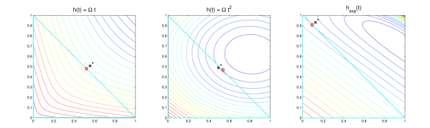
Figure 2: Contour plots of $f=h(\sqrt{x^{\top}Mx})-r^{\top}x$ for different risk-weighting functions.

5 Conclusions

We presented a branch-and-bound algorithm for a large class of convex mixed-integer minimization problems arising in portfolio optimization. Dual bounds are obtained by a modified version of the Frank-Wolfe method. This is motivated mainly by two reasons. On the one hand, the Frank-Wolfe algorithm, at each iteration, gives a valid dual bound for the original mixed-integer problem, therefore it may allow an early pruning of the node. On the other hand, the cost per iteration is very low, since the computation of the descent direction and the update of the objective function can be performed in a very efficient way. Furthermore, the devised Frank-Wolfe method benefits from the use of a non-monotone Armijo line search. Within the branch-and-bound scheme, we propose different warmstarting strategies. The branch-and-bound algorithm has been tested on a set of real-world instances for the capital budgeting problem, considering different classes of risk-weighting functions. Experimental results show that the proposed approach significantly outperforms the MISOCP solver of CPLEX 12.6 for instances where a linear risk-weighting function is considered.

6 Appendix

Proof of Lemma 2:

Proof.

First note that the definition of $\bar{f}^{k}$ ensures $\bar{f}^{k}\leq f(x^{0})$ and hence $f(x^{k})\leq f(x^{0})$ for all $k$, which proves (i). For (ii), we have that

$$\bar{f}^{k+1}=\max\limits_{0\leq i\leq\min\{p_{nm},k+1\}}f(x^{k+1-i})\leq\max\{\bar{f}^{k},f(x^{k+1})\}.$$

Since $f(x^{k+1})<\bar{f}^{k}$ by the definition of the line search, we derive $\bar{f}^{k+1}\leq\bar{f}^{k}$, which proves that the sequence $\{\bar{f}^{k}\}_{k\in\mathbb{N}}$ is non-increasing. By (i), this sequence is bounded from below by the minimum of $f$ on $\mathcal{L}(x^{0})\cap S$, which exists by Lemma 1, and hence converges.

∎

Proof of Lemma 3:

Proof.

For each $k\in\mathbb{N}$, choose $t^{k}\in\{k-\min(k,p_{nm}),\dots,k\}$ with $\bar{f}^{k}=f(x^{t^{k}})$. We prove by induction that for any fixed integer $i\geq 0$ we have

$$\lim_{k\rightarrow\infty}f(x^{t^{k}-i})=\lim_{k\rightarrow\infty}f(x^{t^{k}})=\lim_{k\rightarrow\infty}\bar{f}^{k}=\bar{f}.$$ (13)

Suppose at first $i=0$. Then (13) follows from Lemma 2.

We now assume that (13) holds for $i\geq 0$ and we prove that it holds for index $i+1$. We have

$$f(x^{t^{k}-i})\leq\bar{f}^{t^{k}-i-1}+\gamma_{1}\alpha^{t^{k}-i-1}\nabla f(x^{t^{k}-i-1})^{\top}d^{t^{k}-i-1}-\gamma_{2}(\alpha^{t^{k}-i-1})^{2}\|d^{t^{k}-i-1}\|^{2},$$

so that the same reasoning as before yields

$$f(x^{t^{k}-i})-\bar{f}^{t^{k}-i-1}\leq-\gamma_{2}(\alpha^{t^{k}-i-1})^{2}\|d^{t^{k}-i-1}\|^{2}.$$ (14)

The left hand side of (14) converges to zero since (13) holds for $i$ and the term $f(x^{t^{k}-i})$ converges to $\bar{f}$ (by the inductive hypothesis), as well as $\bar{f}^{t^{k}-i-1}$ because of Lemma 2 (and the fact that $k-(t^{k}-i-1)$ is bounded by $p_{nm}+i+1$). Then,

$$\lim_{k\rightarrow\infty}(\alpha^{t^{k}-i-1})^{2}\|d^{t^{k}-i-1}\|^{2}=0,$$

so that $\lim_{k\rightarrow\infty}\|x^{t^{k}-i}-x^{t^{k}-i-1}\|=0$. Again, uniform continuity of $f(x)$ over $\mathcal{L}(x^{0})\cap S$ yields (13) for index $i+1$.

To conclude the proof, let $T^{k}=t^{k+p_{nm}+1}$ and note that for any $k$ we can write

$$f(x^{k})=f(x^{T^{k}})-\sum_{i=0}^{T^{k}-k-1}(f(x^{T^{k}-i})-f(x^{T^{k}-i-1})).$$

Therefore, since the summation vanishes and $f(x^{T^{k}})=\bar{f}^{k+p_{nm}+1}$ converges to $\bar{f}$ from Lemma 2, taking the limit for $k\rightarrow\infty$ and observing $T^{k}-k-1\leq p_{nm}$ we obtain the result.

∎

Proof of Lemma 4:

Proof.

First note that $\nabla f(x^{k})^{\top}d^{k}<0$ for all $k\in\mathbb{N}$. Let $\alpha^{k}$ be the stepsize used by NM-MFW at iteration $k$. Then,

$$\bar{f}^{k}-f(x^{k}+\alpha^{k}d^{k})\geq\gamma_{1}\,\alpha^{k}\,|\nabla f(x^{k})^{\top}d^{k}|+\gamma_{2}\,(\alpha^{k})^{2}\,\|d^{k}\|^{2}\geq\gamma_{1}\,\alpha^{k}\,|\nabla f(x^{k})^{\top}d^{k}|\geq 0.$$

By Lemma 3, the left hand side converges to zero, hence

$$\lim_{k\rightarrow\infty}\alpha^{k}\,|\nabla f(x^{k})^{\top}d^{k}|=0.$$ (15)

Since $f$ is continuously differentiable on the compact set $\mathcal{L}(x^{0})\cap S$ by Lemma 1 and $d^{k}$ is bounded on $S$, the sequence $\nabla f(x^{k})^{\top}d^{k}$ is bounded. It thus suffices to show that any convergent subsequence of $\nabla f(x^{k})^{\top}d^{k}$ converges to zero.

We assume by contradiction that a subsequence exists with

$$\lim_{i\rightarrow\infty}\nabla f(x^{k_{i}})^{\top}d^{k_{i}}=-\eta<0.$$

Since the sequences $\{x^{k}\}_{k\in\mathbb{N}}$ and $\{d^{k}\}_{k\in\mathbb{N}}$ are bounded, we can switch to an appropriate subsequence and assume that $\lim_{k\rightarrow\infty}x^{k}=\bar{x}$ and $\lim_{k\rightarrow\infty}d^{k}=\bar{d}$ exist. From (15) we obtain

$$\lim_{k\rightarrow\infty}\alpha^{k}=0,$$ (16)

and the continuity of the gradient in $\mathcal{L}(x^{0})\cap S$ implies

$$\nabla f(\bar{x})^{\top}\bar{d}=\lim_{k\rightarrow\infty}\nabla f(x^{k})^{\top}d^{k}=-\eta<0.$$

Since $\alpha_{max}\geq\beta>0$ and the sequence $\alpha^{k}$ is converging to zero, a value $\bar{k}\in\mathbb{N}$ exists such that $\alpha^{k}<\alpha_{max}$, for $k\geq\bar{k}$. In other words, for $k\geq\bar{k}$ the stepsize $\alpha^{k}$ cannot be set equal to the maximum stepsize and, taking into account the non-monotone Armijo line search, we can write

$$f\Big{(}x^{k}+\frac{\alpha^{k}}{\delta}d^{k}\Big{)}>\bar{f}^{k}+\gamma_{1}\,\frac{\alpha^{k}}{\delta}\,\nabla f(x^{k})^{\top}d^{k}-\gamma_{2}\,\Big{(}\frac{\alpha^{k}}{\delta}\Big{)}^{2}\,\|d^{k}\|^{2}.$$

Hence, due to the fact that $\bar{f}^{k}\geq f(x^{k})$, we get

$$f\Big{(}x^{k}+\frac{\alpha^{k}}{\delta}d^{k}\Big{)}-f(x^{k})>\gamma_{1}\,\frac{\alpha^{k}}{\delta}\,\nabla f(x^{k})^{\top}d^{k}-\gamma_{2}\,\Big{(}\frac{\alpha^{k}}{\delta}\Big{)}^{2}\,\|d^{k}\|^{2}.$$ (17)

Since $f$ is continuously differentiable in $\mathcal{L}(x^{0})\cap S$, we can apply the Mean Value Theorem and we have that $s_{k}\in[0,1]$ exists such that

$$f\Big{(}x^{k}+\frac{\alpha^{k}}{\delta}d^{k}\Big{)}=f(x^{k})+\frac{\alpha^{k}}{\delta}\nabla f\Big{(}x^{k}+s_{k}\frac{\alpha^{k}}{\delta}d^{k}\Big{)}^{\top}d^{k}.$$ (18)

In particular, we have $\lim_{k\rightarrow\infty}x^{k}+s_{k}\frac{\alpha^{k}}{\delta}d^{k}=\bar{x}$, by (16) and since $s_{k}$ and $d^{k}$ are bounded. By substituting (18) within (17) we have

$$\nabla f\Big{(}x^{k}+s\frac{\alpha^{k}}{\delta}d^{k}\Big{)}^{\top}d^{k}>\gamma_{1}\,\nabla f(x^{k})^{\top}d^{k}-\gamma_{2}\,\frac{\alpha^{k}}{\delta}\,\|d^{k}\|^{2}.$$

Considering the limit on both sides we get

$$-\eta=\nabla f(\bar{x})^{\top}\bar{d}>\gamma_{1}\,\nabla f(\bar{x})^{\top}\bar{d}=-\gamma_{1}\eta$$

which is a contradiction since $\gamma_{1}\in(0,\frac{1}{2})$ and $-\eta<0$.

∎

Proof of Theorem 1:

Proof.

If NM-MFW does not stop in a finite number of iterations at an optimal solution, from Lemma 4 we have that

$$\lim_{k\rightarrow\infty}\nabla f(x^{k})^{\top}d^{k}=0.$$

Let $x^{\star}$ be any limit point of $\{x^{k}\}_{k\in\mathbb{N}}$. Since the sequence $\{d^{k}\}_{k\in\mathbb{N}}$ is bounded, we can switch to an appropriate subsequence and assume that

$$\lim_{k\rightarrow\infty}x^{k}=x^{\star};\quad\lim_{k\rightarrow\infty}d^{k}=d^{\star}.$$

Therefore

$$\nabla f(x^{\star})^{\top}d^{\star}=\lim_{k\rightarrow\infty}\nabla f(x^{k})^{\top}d^{k}=0.$$

From the definition of $d^{k}$ (implied by (10) and the definition of $d^{TS}$) we have

$$\nabla f(x^{k})^{\top}d^{k}\leq\nabla f(x^{k})^{\top}(x-x^{k})\quad\forall\;x\in S.$$

Taking the limit for $k\rightarrow\infty$ yields

$$0=\nabla f(x^{\star})^{\top}d^{\star}\leq\nabla f(x^{\star})^{\top}(x-x^{\star})\quad\forall\;x\in S,$$

showing that $x^{\star}$ is an optimal solution for Problem (5).

∎

References

- Atamtürk and Narayanan [2008] A. Atamtürk and V. Narayanan. Polymatroids and mean-risk minimization in discrete optimization. Operations Research Letters, 36(5):618–622, 2008.
- Baumann et al. [2014] F. Baumann, C. Buchheim, and A. Ilyina. Lagrangean decomposition for mean-variance combinatorial optimization. In International Symposium on Combinatorial Optimization – ISCO 2014, volume 8596 of LNCS, pages 62–74, 2014.
- Bertsimas and Sim [2004] D. Bertsimas and M. Sim. Robust discrete optimization under ellipsoidal uncertainty sets. Technical report, MIT, 2004.
- Buchheim et al. [2016] C. Buchheim, M. De Santis, S. Lucidi, F. Rinaldi, and L. Trieu. A feasible active set method with reoptimization for convex quadratic mixed-integer programming. SIAM Journal on Optimization, 26(3):1695–1714, 2016.
- Cesarone et al. [2013] F. Cesarone, A. Scozzari, and F. Tardella. A new method for mean-variance portfolio optimization with cardinality constraints. Annals of Operations Research, 205(1):213–234, 2013.
- Clarke [1990] F. H. Clarke. Optimization and nonsmooth analysis, volume 5. Philadelphia: SIAM., 1990.
- Clarkson [2010] K. L. Clarkson. Coresets, sparse greedy approximation, and the Frank-Wolfe algorithm. ACM Transactions on Algorithms, 6(4):63, 2010.
- Dolan et al. [2002] E. Dolan and J. Moré. Benchmarking optimization software with performance profiles, Mathematical Programming, 91:201–213, 2002.
- Duchi et al. [2008] J. Duchi, S. Shalev-Shwartz, Y. Singer, and T. Chandra. Efficient projections onto the l1-ball for learning in high dimensions. In Proceedings of the 25th International Conference on Machine Learning, ICML - 08, pages 272–279, 2008.
- Dunn [1980] J. C. Dunn. Convergence rates for conditional gradient sequences generated by implicit step length rules. SIAM Journal on Control and Optimization, 18(5):473–487, 1980.
- Frank and Wolfe [1956] M. Frank and P. Wolfe. An algorithm for quadratic programming. Naval research logistics quarterly, 3(1-2):95–110, 1956.
- Freund and Grigas [2014] R. M. Freund and P. Grigas. New analysis and results for the Frank-Wolfe method. Mathematical Programming, pages 1–32, 2014.
- Gao [2004] Z. Gao, W. H. K. Lam, S. C. Wong and H. Yang. The Convergence of Equilibrium Algorithms with Non-monotone Line Search Technique. Applied Mathematics and Computation, 148(1): 1–13, 2004
- Grippo et al. [1986] L. Grippo, F. Lampariello, and S. Lucidi. A nonmonotone line search technique for newton’s method. SIAM Journal on Numerical Analysis, 23(4):707–716, 1986.
- Grippo et al. [1989] L. Grippo, F. Lampariello, and S. Lucidi. A truncated newton method with nonmonotone line search for unconstrained optimization. Journal of Optimization Theory and Applications, 60(3):401–419, 1989.
- Grippo and Sciandrone [2002] L. Grippo and M. Sciandrone. Nonmonotone globalization techniques for the Barzilai-Borwein gradient method. Computational Optimization and Applications, 23(2):143–169, 2002.
- Guélat and Marcotte [1986] J. Guélat and P. Marcotte. Some comments on Wolfe’s “away step”. Mathematical Programming, 35(1):110–119, 1986.
- Held et al. [1974] M. Held, P. Wolfe, and H. Crowder. Validation of subgradient optimization. Mathematical Programming, 6(1):62–88, 1974.
- Jaggi [2013] M. Jaggi. Revisiting Frank-Wolfe: Projection-free sparse convex optimization. In Proceedings of the 30th International Conference on Machine Learning, ICML - 13, pages 427–435, 2013.
- Julstrom [2005] B. A. Julstrom. Greedy, genetic, and greedy genetic algorithms for the quadratic knapsack problem. In GECCO, pages 607–614, 2005.
- Lacoste-Julien and Jaggi [2013] S. Lacoste-Julien and M. Jaggi. An affine invariant linear convergence analysis for Frank-Wolfe algorithms. arXiv preprint arXiv:1312.7864, 2013.
- Markowitz [1952] H. Markowitz. Portfolio selection. The Journal of Finance, 7(1):77–91, 1952.