Time-dependent phase shift of a retrieved pulse in off-resonant EIT-based light storage

Abstract

We report measurements of the time-dependent phases of the leak and retrieved pulses obtained in EIT storage experiments with metastable helium vapor at room temperature. In particular, we investigate the influence of the optical detuning at two-photon resonance, and provide numerical simulations of the full dynamical Maxwell-Bloch equations, which allow us to account for the experimental results.

I Introduction

Because they do not interact with each other and can be guided via optical fibers over long distances with relatively low losses, photons appear as ideal information carriers and are therefore put forward as the "flying qubits" in most of quantum communication protocols. The design of memories able to reliably store and retrieve photonic states is, however, still an open problem. The most commonly studied protocol, considered to implement such a quantum memory, is electromagnetically induced transparency (EIT) BIH91 . This protocol was implemented in various systems such as cold atoms, gas cells, or doped crystals LDB01 ; PFM01 ; HLL10 . Although the Doppler broadening might seem to lead to strong limitations, EIT-based light storage in warm alkali vapors gives good results and is still a subject of active investigation NWX12 . In the last years, some experiments were also performed in a Raman configuration, using pulses which are highly detuned from the optical resonances in gas cells RNL10 ; RML11 ; RNJ12 .

The EIT-based storage protocol in a $\Lambda$ atomic system relies on the long-lived Raman coherence between the two ground states which are optically coupled to the excited level. When a strong coupling beam is applied along one of the two transitions, a narrow transparency window limited by the Raman coherence decay rate is opened along the other leg of the system. Because of the slow-light effect associated with such a dramatic change of the medium absorption properties, a weak probe pulse on the second transition is compressed while propagating through the medium. When this pulse has fully entered the atomic medium, it can be mapped onto the Raman coherences which are excited by the two-photon process by suddenly switching off the coupling beam. It can be safely stored during times smaller than the lifetime of Raman coherence. Finally, the signal pulse can be simply retrieved by switching on the coupling beam again. In the Raman configuration, the coupling and probe pulses are optically far off-resonance but still fulfill the two-photon transition condition. The advantage is a large bandwidth, that allows to work with data rates higher than in the usual EIT regime RNL10 .

Atoms at room temperature in a gas cell are particularly attractive for light storage because of the simplicity of their implementation. The effects of the significant Doppler broadening can be minimized using co-propagating coupling and probe beams, so that the two-photon resonance condition can be verified for all velocity classes: all the atoms can thus participate to the EIT phenomenon as soon as they are pumped in the probed level. As a consequence, handy simple gas cells have turned out to be attractive for slow or even stopped light experiments NWX12 . In a previous work MLM14 , we have reported on an added phase shift recorded for EIT-based light storage experiments carried out in a helium gas at room temperature when the coupling beam is detuned from the center of the Doppler line. The simple model that we have derived could not satisfactorily account for our observations that were recorded for intermediate detunings, e.g. close to the Doppler broadening of the transition. In the present paper, we come back to this problem and provide new experimental results, i.e. time-dependent measurements of the retrieved signal phase shift, as well as numerical results obtained through the simulation of the full system of Maxwell-Bloch equations. The behaviour of these phase shifts with the coupling detuning seems satisfactorily accounted for by our simulations. We also perform numerical calculations in the Raman regime.

The paper is organized as follows. In Section II we present the system and setup and describe how to measure the time-dependent phase shift of the retrieved pulse with respect to the coupling beam. We also briefly recall the system of Maxwell-Bloch equations which governs our system and describe their numerical integration. In Section III, we provide our experimental and numerical results and show that they qualitatively agree. We also apply our simulations to the far off-resonant Raman case. Finally, we conclude in Section IV and give possible perspectives of our work.

II Experimental setup and numerical simulations

II.1 EIT storage experimental setup

The atoms preferably used for EIT storage experiments are alkali atoms, mainly rubidium and sometimes sodium or caesium. We choose here to work with metastable ⁴He atoms, which have the advantage of a very simple structure without hyperfine levels: transitions are thus far enough one from another to investigate the effect of detunings of the coupling and probe beams on light storage and retrieval.

In our setup represented in Fig. 1, a $6$-cm-long cell is filled up with $1$ Torr of helium atoms which are continuously excited to their metastable state $2^{3}S_{1}$ by a radio-frequency (rf) discharge at 27 MHz. Each of the metastable ground states $\left|2^{3}S_{1},m_{J}=0,\pm 1\right\rangle$ is hence fed with the same rate, denoted by $\frac{\Lambda}{3}$. The cell is isolated from magnetic field gradients by a three-layer $\mu$-metal shield to avoid spurious dephasing effects on the different Zeeman components. A strong circularly-polarized field, called the control beam, propagates along the quantization axis $z$. Its power is set at $18$ mW for a beam diameter of $3$ mm. As shown in Fig. 2, the coupling field drives the transitions $\left|2^{3}S_{1},m_{J}=-1\right\rangle\leftrightarrow\left|2^{3}P_{1},m_{J}=0\right\rangle$ and $\left|2^{3}S_{1},m_{J}=0\right\rangle\leftrightarrow\left|2^{3}P_{1},m_{J}=1\right\rangle$. Owing to the spontaneous transitions $\left|2^{3}P_{1},m_{J}=0\right\rangle\rightarrow\left|2^{3}S_{1},m_{J}=\pm 1\right\rangle$ and $\left|2^{3}P_{1},m_{J}=1\right\rangle\rightarrow\left|2^{3}S_{1},m_{J}=0,1\right\rangle$, the atoms end up in the state $\left|1\right\rangle\equiv\left|2^{3}S_{1},m_{J}=1\right\rangle$ within a few pumping cycles after the coupling beam has been switched on. As the atoms are at room temperature, the Doppler broadening in the cell is $W_{D}/2\pi\approx 1\,\mbox{GHz}$. We denote by $\Delta_{c}\equiv\omega_{c}-\omega_{0}$ the detuning of the coupling frequency $\omega_{c}$ with respect to the natural frequency $\omega_{0}/(2\pi)\approx 2.8\times 10^{14}\,\mbox{Hz}$ of the transition $2^{3}S_{1}\leftrightarrow 2^{3}P_{1}$, at the center of the Doppler line.

Once optical pumping is achieved, a weak signal pulse is sent through the atomic medium along the $z$ axis. Its polarization is circular and orthogonal to that of the coupling beam: the signal therefore couples the state $\left|1\right\rangle$ to $\left|e\right\rangle\equiv\left|2^{3}P_{1},m_{J}=0\right\rangle$ and we denote by $\Delta_{s}\equiv\omega_{s}-\omega_{0}$ the detuning of the signal frequency $\omega_{s}$ from the center of the Doppler profile. Both signal and coupling beams are derived from the same laser diode, and their frequencies and amplitudes are controlled by two acousto-optic modulators. Due to the efficiency of optical pumping through the coupling beam, we assume that the state $\left|2^{3}S_{1},m_{J}=0\right\rangle$ remains essentially unpopulated during the whole process and we accordingly neglect the driving of the transition $\left|2^{3}S_{1},m_{J}=0\right\rangle\leftrightarrow\left|2^{3}P_{1},m_{J}=-1\right\rangle$ by the signal field. Submitted to the coupling and signal fields, the atoms therefore essentially evolve in the three-level $\Lambda$ system $\left\{\left|-1\right\rangle\equiv\left|2^{3}P_{1},m_{J}=-1\right\rangle,\left|e\right\rangle,\left|1\right\rangle\right\}$ (see Fig. 2) as long as the detunings $\Delta_{c,s}=\omega_{c,s}-\omega_{0}$, of the coupling and signal fields respectively, are small enough to avoid exciting neighbouring transitions. Thanks to the absence of hyperfine structure, the range of allowed values for $\Delta_{c,s}$ is, however, much larger than in alkali vapor experiments: indeed, on the positive detuning side the nearest state (${}^{3}P_{0}$) is $30$ GHz away from optical resonance $\Delta_{c,s}=0$, while, on the negative detuning side, the nearest state (${}^{3}P_{2}$) is $2.29$ GHz away.

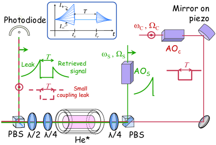
Figure 1: Experimental setup for EIT storage in metastable helium. The coupling and signal beams are derived from the same laser diode. They are initially linearly and orthogonally polarized, of optical frequencies $\omega_{c}$ and $\omega_{s}$ and Rabi frequencies $\Omega_{c}$ and $\Omega_{s}$, respectively. Acousto-optic modulators are used to control the frequencies and amplitudes of the beams. Polarizing Beam Splitters (PBS) allow to separate or recombine the beams. Circular orthogonal polarizations are obtained by a quarter wave-plate. The cell is contained into a $\mu$-metal shielding. After the cell, polarization optics select mainly the probe beam with some remaining coupling beam.The phase of the coupling beam is scanned thanks to a mirror on a piezo-electric tranducer.

Under EIT conditions, the coupling beam opens a transparency window for the weak signal beam, which can therefore propagate without absorption through the medium if its spectrum is not too wide FIM05 . In the experimental results we present hereafter, we used a signal pulse, which consists of a smoothly increasing exponential followed by an abruptly decaying exponential of respective characteristic times $2\,\mu\mbox{s}$ and $150$ ns. Its maximum power is about $170\,\mu\mbox{W}$ and the beam diameter is about $3$ mm. Different dissipative mechanisms influence the width of the EIT window besides spontaneous emission, such as collisions and transit of the atoms in and out of the beams. These phenomena result in the decay of atomic coherences at the rates $\gamma_{-11}/2\pi\approx 14\,$kHz for the Raman coherence $\sigma_{-11}$ and $\gamma_{e1}/2\pi\approx 22.8\mbox{ MHz}$ for the optical coherence $\sigma_{e1}$. We have shown previously that velocity changing collisions redistribute the pumping of the atoms over an effective width sligthly smaller than the Doppler linewidth GGG09 . In our conditions, with a coupling power of 18 mW, this effective width is experimentally estimated to be $\Gamma_{D}/2\pi\approx 0.8\,$GHz. Due to power broadening, the width of the transparency window is then of the order of $500$ kHz.

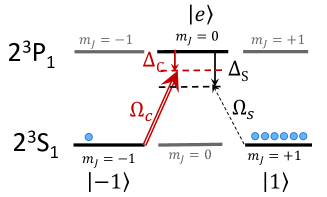
Figure 2: Atomic structure scheme for the D1 transition of metastable helium. The relevant states which constitute the three-level $\Lambda$ system are shown in black. $\Delta_{c}$ and $\Delta_{s}$ are the optical detunings, and $\Omega_{c}$ and $\Omega_{s}$ the Rabi frequencies of the coupling and signal beams, respectively. The two photon resonance is achieved for $\Delta_{c}=\Delta_{s}$.

The highly dispersive character of the medium under EIT conditions can be used furthermore to store and retrieve a weak signal pulse: due to EIT dispersion, the signal pulse indeed travels with a reduced group velocity and is temporally contracted. Once the pulse has entered the cell, the coupling beam can be switched off: information about the signal pulse is then stored into the Raman coherences. After a storage time $T$, the control beam is switched on again, which releases the signal from the atomic coherence and ensures EIT absorption-free propagation. Note that in our experimental setup, the optical depth is only about 3.5 and the pulse can thus not be fully compressed in the cell. Due to the finite width of the transparency window and the finite length of the cell, a part, typically $10$ % of the incoming signal energy, leaks out before the coupling beam is turned off and the storage period begins NWX12 . A typical experimental record is given in Fig. 3b. The first part of the detected signal is the leak and after a storage time $T\approx 0.6\,\mu$s, once the coupling beam is turned on again, the retrieved signal is clearly visible.

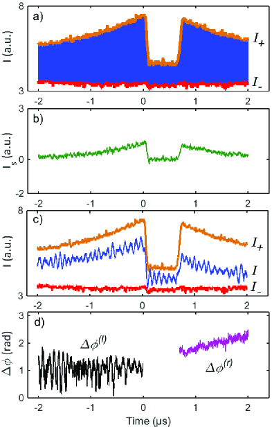
Figure 3: (Color online) Experimental plots showing the data processing steps. The coupling beam is switched off between times $t=0$ and $t=0.6\,\mu$s. The optical detunings are set at $\Delta_{c,s}=1$ GHz. The same vertical scale is used in graphs a, b and c. a) Accumulated plot of the interference signal $I(t)$ between the probe and coupling beams (blue). Upper and lower envelopes $I_{\pm}\left(t\right)$ are shown in orange and red, respectively. b) Signal intensity $I_{s}\left(t\right)$ at the exit of the cell, deduced from the previous accumulated plot a) and from a measurement of the coupling intensity $I_{c}$. c) Interference signal $I(t)$ between the probe and coupling beams (blue). It is contained between the upper and lower envelopes $I_{\pm}\left(t\right)$, shown in orange and red, respectively. One can note the presence of spurious oscillations generated by the acousto-optic modulators. d) Relative phases $\Delta\phi^{(l)}(t)$ (black) and $\Delta\phi^{(r)}(t)$ (purple) between the signal and coupling beams on the writing and retrieval parts, respectively. Notice that $\Delta\phi^{(l)}(t)$ is indeed constant.

II.2 Phase measurement setup

In MLM14 , we investigated the relative phase $\Delta\phi$ of the signal with respect to the coupling beam, and showed the existence of an optical detuning dependent extra phase shift $\varphi_{EIT}$ between the incident and retrieved pulse. This quantity can be measured through mixing the signal emerging from the cell with a small fraction of the control beam, via polarization optics. The resulting intensity thus takes the form

$$I=I_{c}+I_{s}+\alpha\sqrt{I_{c}I_{s}\left(t\right)}\cos\left[\Delta\phi\right].$$ (1)

In Eq. (1), the contrast factor $\alpha$, which ideally equals $2$, accounts for non-perfect alignment of the beams and is measured for each set of data. $I_{c}$ denotes the intensity of the small fraction of the coupling field which is mixed and interferes with the signal field. It takes the same constant value $I_{c}$ during the writing and retrieval periods, while it vanishes during the storage time. The value $I_{c}$ is measured in the absence of the signal (one assumes that the introduction of the signal pulse does not substantially affect the measurement of $I_{c}$). The phase of the coupling beam is varied via a piezoelectric actuator from one experimental run to another: the scan is slow enough so that it is assumed to be constant during both the writing or retrieval steps. $I_{s}\left(t\right)$ is the time-dependent intensity of the signal beam emerging from the cell. We denote by $I_{s}^{(l)}(t)$ and $I_{s}^{(r)}(t)$ the intensities of the leak and retrieved pulses, respectively. Accordingly, we introduce $\Delta\phi^{(l)}(t)$ and $\Delta\phi^{(r)}(t)$, the relative phases of the leak and retrieved pulses, with respect to the coupling beam.

To obtain the extra phase shift $\varphi_{EIT}$ between the incident and retrieved pulses, we measure the relative phases $\Delta\phi^{(l)}$, $\Delta\phi^{(r)}$ by homodyne detection. Repeating the same writing-storage-retrieval sequence for many different postions of the piezoelectric actuator, we obtain an accumulated plot whose upper/lower envelopes correspond respectively to $I_{\pm}\left(t\right)=I_{c}+I_{s}\left(t\right)\pm\alpha\sqrt{I_{c}I_{s}\left(t\right)}$ (see Fig. 3a). Given the previously measured value of $I_{c}$, one can infer $I_{s}\left(t\right)$ from $\left(I_{+}+I_{-}\right)$ and $\alpha$ from $\left(I_{+}-I_{-}\right)$ (see Fig. 3b). For a given position of the piezo-actuator, one can then obtain $\Delta\phi^{(l)}(t)$ and $\Delta\phi^{(r)}(t)$ through fitting the experimental record with Eq. (1) at each time $t$ (see Figs. 3c, d). It was verified both experimentally and numerically that the phase of the leak is constant ($\Delta\phi^{(l)}(t)\equiv\Delta\phi^{(l)}$) and can therefore be taken as a reference for the time-dependent relative phase of the retrieved pulse $\Delta\phi^{(r)}(t)$. This time independence of the leak phase is ensured by the fact that its spectral content is much narrower than the EIT bandwidth. This is obtained thanks to the shape of the signal pulse: a slow exponential increase, followed by a sharp decrease. The part of the pulse which contains only low frequencies enters first and gives form to a leak, whose phase is constant. The “extra phase shift” is then measured as $\left[\Delta\phi^{(r)}(t)-\Delta\phi^{(l)}\right]\equiv\varphi_{EIT}(t)$. Let us stress that in MLM14 , we assumed that the relative phases $\Delta\phi^{\left(l,r\right)}$ of the leak and retrieved pulses were time-independent: therefore, we directly extracted effective “averaged” values for $\alpha$ and $\varphi_{EIT}$ by performing a two-parameter fit of the data with Eq. (1). Here, by contrast, we measure the time-dependence of the phases and provide experimental plots for $\varphi_{EIT}(t)$, without any assumption on its behaviour.

II.3 Numerical simulation principles

For numerical simulations, we described the system in the one-dimensional approximation. On the dimensions of the atomic sample, the coupling and probe transverse profiles are assumed to remain constant. These fields can therefore be cast under the form

$$\mathbf{E}_{c,s}\left(z,t\right) = \Re\left[\mathcal{E}_{c,s}\left(z,t\right)\mathbf{e}_{\pm}e^{-\mathrm{i}\left(\omega_{c,s}t-k_{c,s}z\right)}\right]\mbox{, }$$

where $\mathcal{E}_{c,s}\left(z,t\right)$ denote the respective slowly-varying amplitudes of the control and signal fields, $\omega_{c,s}$ and $k_{c,s}$ stand for their respective frequencies and wavenumbers, while $\mathbf{e}_{\pm}\equiv(\mathbf{e}_{x}\pm\mbox{i}\mathbf{e}_{y})/\sqrt{2}$ ($\mathbf{e}_{x}$ and $\mathbf{e}_{y}$ define an arbitrary basis in the plane perpendicular to the propagation direction $\mathbf{e}_{z}$).

Following e.g. GAL07 , we model the atomic sample as a continuous medium of uniform linear density $n_{at}$, and define the average density matrix of the slice $\left[z,z+\Delta z\right]$ by

$$\mathbf{\hat{\sigma}}\left(z,t\right)\equiv\frac{1}{n_{at}\Delta z}\sum_{z\leq z_{i}\leq z+\Delta z}\hat{\sigma}_{i}\left(t\right)\mbox{. }$$

We moreover define the density matrix elements $\sigma_{ij}=\left\langle i\left|\hat{\sigma}\right|j\right\rangle$ where $i,\,j$ refer to the atomic levels and can take the values $-1,\,1$ or $e$ (see Fig. 2). We introduce the slowly-varying coherences $\tilde{\sigma}_{e1},\,\tilde{\sigma}_{e-1}$ and $\tilde{\sigma}_{-11}$ defined by:

$$\tilde{\sigma}_{e1} =e^{\textrm{\mbox{\mbox{i}}}\omega_{s}\left(t-\frac{z}{c}\right)}\sigma_{e1},$$

$$\tilde{\sigma}_{e-1} \equiv e^{\textrm{\mbox{\mbox{i}}}\omega_{c}\left(t-\frac{z}{c}\right)}\sigma_{e-1},$$

$$\tilde{\sigma}_{-11} \equiv e^{\textrm{\mbox{\mbox{\mbox{\mbox{i}}}}}\Delta_{R}\left(t-\frac{z}{c}\right)}\sigma_{-11},$$

and write the Bloch equations in the rotating wave approximation, for the class of velocity which is at the center of the Doppler profile:

$$\partial_{t}\sigma_{-1-1} = \frac{\gamma_{t}}{3}-\gamma_{t}\sigma_{-1-1}+\frac{\Gamma_{0}}{2}\sigma_{ee}+\mbox{i}\left(\Omega_{c}^{*}\tilde{\sigma}_{e-1}-\Omega_{c}\tilde{\sigma}_{-1e}\right),$$ (2)

$$\partial_{t}\sigma_{ee} = -\left(\Gamma_{0}+\gamma_{t}\right)\sigma_{ee}+\mbox{i}\left(\Omega_{c}\tilde{\sigma}_{-1e}-\Omega_{c}^{*}\tilde{\sigma}_{e-1}+\Omega_{s}\tilde{\sigma}_{1e}-\Omega_{s}^{*}\tilde{\sigma}_{e1}\right),$$ (3)

$$\partial_{t}\sigma_{11} = \frac{2\gamma_{t}}{3}-\gamma_{t}\sigma_{11}+\frac{\Gamma_{0}}{2}\sigma_{ee}+\mbox{i}\left(\Omega_{s}^{*}\tilde{\sigma}_{e1}-\Omega_{s}\tilde{\sigma}_{1e}\right),$$ (4)

$$\partial_{t}\tilde{\sigma}_{-11} = -\left(\gamma_{-11}-\mbox{i}\Delta_{R}\right)\tilde{\sigma}_{-11}+\mbox{i}\left(\Omega_{c}^{*}\tilde{\sigma}_{e1}-\Omega_{s}\tilde{\sigma}_{-1e}\right),$$ (5)

$$\partial_{t}\tilde{\sigma}_{-1e} = -\left(\gamma_{-1e}+\mbox{i}\Delta_{c}\right)\tilde{\sigma}_{-1e}+\mbox{i}\left[\Omega_{c}^{*}\left(\sigma_{ee}-\sigma_{-1-1}\right)-\Omega_{s}^{*}\tilde{\sigma}_{-11}\right],$$ (6)

$$\partial_{t}\tilde{\sigma}_{1e} = -\left(\gamma_{1e}+\mbox{i}\Delta_{s}\right)\tilde{\sigma}_{1e}+\mbox{i}\left\{\Omega_{s}^{*}\left(\sigma_{ee}-\sigma_{11}\right)-\Omega_{c}^{*}\tilde{\sigma}_{1-1}\right\}.$$ (7)

Here, $\Gamma_{0}$ is the population decay rate of the state $\left|e\right\rangle$, and the Rabi frequencies $\Omega_{c,s}$ are defined by

$$\hbar\Omega_{c,s} \equiv \frac{1}{2}d_{c,s}\mathcal{E}_{c,s}\left(z,t\right)\mbox{, }$$

where $d_{c,s}\equiv\left\langle e\left|\hat{\mathbf{d}}.\mathbf{e}_{\pm}\right|\mp 1\right\rangle$ are the relevant matrix elements of the dipole operator $\hat{\boldsymbol{d}}$.

To take into account all the atoms that are distributed in different velocity classes over the Doppler linewidth, we developed a simple model, in which the optical coherence decay rates $\gamma_{1e}=\gamma_{-1e}$ are replaced by the effective Doppler width $\Gamma_{D}$. This gives satisfactory results thanks to the redistribution of the pumping by velocity changing collisions GGD08 ; FVA06 . All our simulations were performed using this purely homogeneous broadening model. Consequently, we call $\Delta_{c,s}$ the optical detuning, implicitly defined with respect to the center of the Doppler profile.

To ensure that the full population remains constant, the discharge-assisted ground-state feeding rate $\Lambda$ has been set to $\gamma_{t}$, the transit rate of the atoms through the laser beam. Moreover, while the state $\left|-1\right\rangle$ is fed with the rate $\frac{\Lambda}{3}=\frac{\gamma_{t}}{3}$, the state $\left|1\right\rangle$ is effectively fed with the rate $\approx\frac{2\Lambda}{3}=\frac{2\gamma_{t}}{3}$. As can be checked by considering the full 6-level system including not only the $\Lambda$ system of interest but also the states $\left|2^{3}S_{1},m_{J}=0\right\rangle,\left|2^{3}P_{1},m_{J}=\pm 1\right\rangle$, the state $\left|1\right\rangle$ is indeed directly fed by the rf discharge with the rate $\frac{\Lambda}{3}$, but also indirectly via the state $\left|2^{3}S_{1},m_{J}=0\right\rangle$ whose population is (almost) immediately transferred to $\left|1\right\rangle$ through optical pumping.

Finally, in the medium, the fields propagate according to the Helmholtz equation, written in the slowly-varying envelope approximation

$$\left(\frac{\partial}{\partial z}+\frac{1}{c}\frac{\partial}{\partial t}\right)\Omega_{c,s}\left(z,t\right)=\mathrm{i}\eta_{c,s}\tilde{\sigma}_{e\mp 1}\left(z,t\right),$$ (8)

where $\eta_{c,s}\equiv(n_{at}k_{c,s}|d_{c,s}|^{2})/(2\hbar\epsilon_{0})$.

The set of Maxwell-Bloch equations Eqs (2-8) was numerically solved in Matlab using the Lax discretization method NumRec . The medium was split into $100$ spatial steps of $0.6\mbox{ mm}$ while the whole storage/retrieval sequence was split into $6\times 10^{6}$ timesteps of $2$ ps. We present and discuss our numerical results in the following section.

III Results and discussion

All the experimental results and simulations are performed at two-photon resonance, which means that the coupling and signal optical detunings are equal. Fig. 4 shows experimental records for the time-dependent extra phase shift $\varphi_{EIT}(t)$, achieved with different values of the optical detunings $\Delta=\Delta_{c}=\Delta_{s}$, between $0$ and $2$ GHz. The detunings are set here on the positive side, where the nearest state (${}^{3}P_{0}$) is nearly $30$ GHz away. Each curve is obtained after averaging over 15 sets of data, recorded at different times, for different positions of the homodyne detection piezo-actuator. The traces recorded on the oscilloscope present some spurious oscillations at a period of about $90$ ns. This noise is generated by the acousto-optic modulators and could be removed by numerically filtering the spurious frequencies during the data processing. In Fig. 4, the time origin corresponds to the begining of the retrieval, when the coupling beam is turned on again. At that time, the probe intensity starts increasing to form the retrieved pulse. We only plot the evolution of the extra phase shift $\varphi_{EIT}(t)$ when the signal intensity is high enough, typically from roughly $100$ ns to $1\,\mu\mbox{s}$ after the start of the retrieval. One can see that $\varphi_{EIT}(t)$ is not constant over the retrieval, and its magnitude increases with the optical detuning $\Delta$.

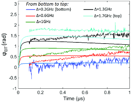
Figure 4: Temporal evolution of the extra phase shift $\varphi_{EIT}(t)$. Experimental data, recorded from bottom to top: for $\Delta=0.2$ GHz (blue, bottom), $0.6$ GHz (red), $1$ GHz (green), $1.3$ GHz (black), $1.7$ GHz (cyan, top). Corresponding simulations are shown as continuous lines. The time origin corresponds to the begining of the retrieval, when the coupling is switched on again. The storage time is set at $T=0.6\,\mu$s.

The experimental plots are compared with numerical simulations of the full Maxwell-Bloch equations derived as explained in the previous section. These simulations are in good agreement with experimental results: both present the same general shape for $\varphi_{EIT}\left(t\right)$, and the same qualitative behaviour with the optical detuning $\Delta$. One possible source for the observed discrepancies is our oversimplified treatment of the velocity distribution in the Doppler profile. Here, we indeed assumed that velocity changing collisions are efficient enough to instantaneously and perfectly redistribute atoms pumped in the probed level $\left|1\right\rangle$ over the effective Doppler profile so that all these atoms contribute coherently to the storage process as if the broadening were homogeneous. Although this approximation is commonly used (see GGD08 ; FVA06 ), it might be severely questioned here, especially in optically detuned conditions that change the thermal equilibrium. In particular, the absorption of the coupling beam measured experimentally could not be well reproduced by the simulations. This should also have an effect on the storage efficiency and on the temporal shape of the phase. Note that in the simulation program, in order to “minimize” this problem, we use an averaged coupling intensity over the length of the cell as the input parameter, instead of the real coupling intensity measured at the entrance of the cell. Note also that we have checked our numerical results agree with the analytic approximate solutions presented in GAL07 .

To understand better the physical origin of the extra phase-shift $\varphi_{EIT}(t)$, we compared the time-dependent relative phase $\Delta\phi\left(t\right)$ between the signal and coupling beams at the exit of the cell, obtained: i) during the storage and retrieval of a weak signal pulse ($\Delta\phi(t)=\Delta\phi^{(l)}(t)$ before $t=0$ and $\Delta\phi(t)=\Delta\phi^{(r)}(t)$ after the storage time $T=0.6\,\mu\mbox{s})$, and ii) during the direct EIT-propagation of the same weak pulse in the medium, while the coupling amplitude remains constant. To compute $\Delta\phi(t)$ in case i), we used the full simulation of Maxwell-Bloch set of equations, whereas in case ii) we simply propagated each spectral component $\omega$ of the incoming pulse with the corresponding susceptibility $\chi\left(\omega\right)$. Fig. 5 simultaneously displays the results we obtained in both cases, for two different values of the optical detuning $\Delta=0.2,\,1.7\mbox{ GHz}$. The shape and order of magnitude for $\Delta\phi\left(t\right)$ are clearly the same in cases i, ii): the main effect of the storage is to introduce a delay corresponding to the storage time $T$ . Here we chose $T=0.6\,\mu\mbox{s},$ but we checked both experimentally and theoretically that this phase shift does not depend on this storage time. This suggests that the observed extra phase shift $\varphi_{EIT}$ is essentially due to the propagation under EIT conditions. Indeed, the stored part presents a sharp decrease associated with many frequency components, and is thus very sensitive to dispersive effects. This problem should be taken into account for high speed information applications, like experiments performed in the Raman configuration RNL10 ; RML11 ; RNJ12 . We have thus performed simulations in the far detuned regime as presented on Fig. 6. The simulation results shown here are plotted for three different optical detunings $\Delta=10$ GHz, $\Delta=15$ GHz, $\Delta=20$ GHz, much higher than the $\Gamma_{D}\approx 0.8\,$GHz Doppler broadening. They were obtained for a number of atoms $n_{at}$ which is $10$ times higher than in our experimental case, and for a coupling power of $200$ mW. These simulation results demonstrate a similar effect on the retrieved signal pulse phase, even slightly stronger than in our experimental conditions. We have also checked that our numerical results in the Raman configuration agree with the analytic approximate solutions presented in GAL07 .

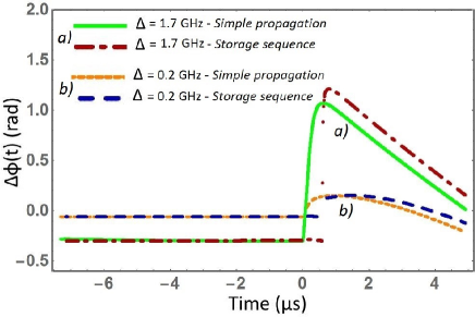
Figure 5: Temporal evolution of the relative phase $\Delta\phi(t)$ during the direct propagation of a weak signal pulse through the medium under EIT conditions (“Simple propagation”) and during the storage and retrieval of the same pulse (“Storage sequence”), for two different optical detunings: a) $1.7$ GHz and b) $0.2$ GHz. The time origin is arbitrarily chosen as the starting of the storage period.

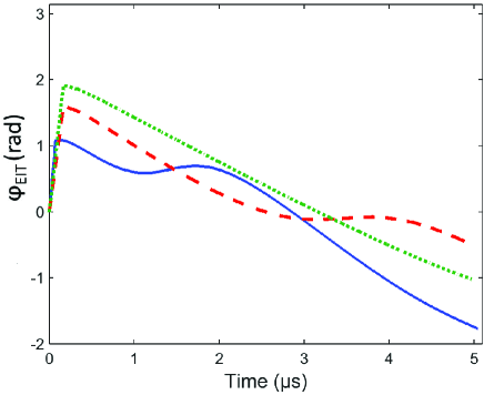
Figure 6: Temporal evolution of the phase shift $\varphi_{EIT}(t)$, for different optical detunings in the Raman regime: $\Delta=10$ GHz (blue, full line), $\Delta=15$ GHz (red, dashed line), $\Delta=20$ GHz (green, dotted line). These curves are obtained with the full simulation of Maxwell-Bloch set of equations, for ten times more atoms than in our experimental case, and for a coupling power of $200$ mW. The time origin is chosen as the starting of the retrieval period.

IV Conclusion

In this paper, we have experimentally investigated a time-dependent extra phase shift that appears in a storage-retrieval experiment, performed in a room temperature atomic cell, in optically detuned conditions. This phase shift varies with time and does not depend on the storage time. We have provided numerical simulations which qualitatively agree with the experimental results: in particular, it appears that the magnitude of the relative phase depends on the optical detuning, while its temporal shape is mainly given by the spectrum of the incoming pulse. We explain the existence of this extra-phase by propagation effects that can be understood by a simple propagation model under EIT conditions with optically detuned beams. Discrepancies may be due to an approximate treatment of Doppler broadening in the cell.

The results presented here might be of importance, particularly for light storage experiments performed in the far-detuned Raman regime, as reported in RML11 . How these results translate into the regime of quantum light is an intriguing feature that we intend to address in a future work.

- (1) K.-J. Boller, A. Imamoglu and S. E. Harris, Phys. Rev. Lett. 66, 2593 (1991).
- (2) C. Liu, Z. Dutton, C. H. Behroozi and L. V. Hau, Nature 409, 490 (2001).
- (3) D. F. Phillips, M. Fleischhauer, A. Mair, R. L. Walsworth and M. D. Lukin, Phys. Rev. Lett. 86, 783 (2001).
- (4) M. P. Hedges, J. J. Longdell, Y. Li and M. J. Sellars, Nature 465, 1052 (2010).
- (5) I. Novikova, R. L. Walsworth and Y. Xiao, Laser Photon. Rev. 6, 633 (2012).
- (6) K. F. Reim, J. Nunn, V. O. Lorenz, B. J. Sussman, K. C. Lee, N. K. Langford, D. Jaksch and I. A. Walmsley, Nature Photon. Lett. 4, 218-221 (2010).
- (7) K. F. Reim, P. Michelberger, K. C. Lee, J. Nunn, N. K. Langford and I. A. Walmsley, Phys. Rev. Lett. 107 053603, (2011).
- (8) K. F. Reim, J. Nunn, X.-M. Jin, P. S. Michelberger, T. F. M. Champion, D. G. England, K. C. Lee, W. S. Kolthammer, N. K. Langford and I. A. Walmsley, Phys. Rev. Lett. 108, 263602 (2012).
- (9) M.-A. Maynard, T. Labidi, M. Mukhtar, S. Kumar, R. Ghosh, F. Bretenaker and F. Goldfarb, EPL 105, 44002 (2014).
- (10) A. V. Gorshkov, A. André, M. D. Lukin and A. S. Sørensen, Phys. Rev. A 76, 033805 (2007).
- (11) M. Fleischhauer, A. Imamoglu and J. P. Marangos, Rev. Mod. Phys. 77, 633 (2005).
- (12) J. Ghosh, R. Ghosh, F. Goldfarb, J.-L. Le Gouët and F. Bretenaker, Phys. Rev. A 80, 023817 (2009).
- (13) A. V. Gorshkov, A. André, M. Fleischhauer, A. S. Sørensen, and M. D. Lukin, Phys. Rev. Lett. 98, 123601 (2007).
- (14) W. H. Press, S. A. Teukolsky, T. Vetterling, B. P. Flannery, “Numerical Recipes in C”, Cambridge University Press (1988).
- (15) F.Goldfarb, J. Ghosh, M. David, J. Ruggiero, T. Chanelière, J.-L. Le Gouët, H. Gilles, R. Ghosh, F. Bretenaker, EPL. 82, 54002 (2008).
- (16) E. Figueroa, F. Vewinger, J. Appel, A. I. Lvovsky, Opt. Lett. 31, 2625-2627 (2006).