Distributed Coordinated Control of Large-Scale Nonlinear Networks

Abstract

We provide a distributed coordinated approach to the stability analysis and control design of large-scale nonlinear dynamical systems by using a vector Lyapunov functions approach. In this formulation the large-scale system is decomposed into a network of interacting subsystems and the stability of the system is analyzed through a comparison system. However finding such comparison system is not trivial. In this work, we propose a sum-of-squares based completely decentralized approach for computing the comparison systems for networks of nonlinear systems. Moreover, based on the comparison systems, we introduce a distributed optimal control strategy in which the individual subsystems (agents) coordinate with their immediate neighbors to design local control policies that can exponentially stabilize the full system under initial disturbances. We illustrate the control algorithm on a network of interacting Van der Pol systems.

1 Introduction

Distributed coordinated control has recently provided powerful control solutions when the conventional centralized methods fail due to inevitable communication constraints and limited computational capabilities. Paradigmatic examples are provided by cooperative and coordinated control for autonomous multi-agent systems (see Bullo et al. (2009)) or large scale interconnected systems (see Zečević and Šiljak (2010)). Distributed coordinated control uses local communications between agents to achieve global objectives that reflect the desired behavior of the multi-agent system. Usually, a two-level hierarchical multi-agent system is employed, which consists of upper level agent for implementing coordinated control and lower level agents for implementing decentralized control. In this paper, we propose to use this conceptual framework to design distributed coordinated control of large scale interconnected system using vector Lyapunov functions (see Bellman (1962); Bailey (1966)) and comparison principles (see Brauer (1961); Beckenbach and Bellman (1961)). The formulations using vector Lyapunov functions are computationally very attractive because of their parallel structure and scalability. However computing these comparison equations, for a given interconnected system, still remained a challenge. In this work we use sum-of-squares (SOS) methods to study the stability of an interconnected system by computing the vector Lyapunov functions as well as the comparison equations. While this approach is applicable to any generic dynamical system, we choose a randomly generated network of modified Van der Pol oscillators for illustration. This network is decomposed into many interacting subsystems and each subsystem parameters are chosen so that individually each subsystem is stable, when the disturbances from neighbors are zero. SOS based expanding interior algorithm (see Jarvis-Wloszek (2003); Anghel et al. (2013)) is used to obtain estimate of region of attraction as sub-level sets of polynomial Lyapunov functions for each such subsystem. Finally SOS optimization is used to compute the stabilizing control policies, based on linear comparison systems, such that the closed-loop network is exponentially stable under initial disturbances.

Following some brief background in Section 2 we formulate the control design problem in Section 3. The sum-of-squares based distributed control algorithm is proposed in Section 4. In Section 5 we illustrate the control design on a network of Van der Pol systems, before concluding the article in Section 6.

2 Preliminaries

2.1 Stability and Control of Nonlinear Systems

Let us consider the dynamical systems of the form

$$\dot{x}\left(t\right)=f\left(x\left(t\right)\right)+u_{t}\,,\quad t\geq 0\,,~{}~{}f(0)=0\,,$$ (1)

where $x\!\in\!\mathbb{R}^{n}$ are the states, $u_{t}\!\in\!\mathbb{R}^{n}$ are the control input, $f:\mathbb{R}^{n}\rightarrow\mathbb{R}^{n}$ is locally Lipschitz and the origin is an equilibrium point of the ‘free’ system, i.e. the system with no control ($u_{t}\equiv 0$). Let us first review the important concepts on stability of the equilibrium point of the ‘free’ system.

Definition 1

The equilibrium point at the origin is called asymptotically stable in a domain $\mathcal{D}\!\subseteq\!\mathbb{R}^{n},\,0\!\in\!\mathcal{D},$ if

$$\left\|x(0)\!\right\|_{2}\ \!\!\!\!\in\!\!\mathcal{D}\implies\lim_{t\rightarrow\infty}\left\|x(t)\right\|_{2}\!=\!0\,,$$

and it is exponentially stable if there exists $b,c\!>\!0$ such that

$$\left\|x(0)\!\right\|_{2}\ \!\!\!\!\in\!\!\mathcal{D}\!\!\!\implies\!\!\!\!\left\|x(t)\right\|_{2}\!<\!ce^{-bt}\!\left\|x(0)\right\|_{2}~{}\forall t\!\geq\!0\,.$$

Lyapunov’s first or direct method (see Lyapunov (1892); Slotine et al. (1991)) can give a sufficient condition of stability through the construction a certain positive definite function.

Theorem 1

If there exists a domain $\mathcal{D}\!\!\in\!\!\mathbb{R}^{n}$, $0\!\!\in\!\!\mathcal{D}$, and a continuously differentiable positive definite function $\tilde{V}\!\!:\!\!\mathbb{R}^{n}\!\rightarrow\!\mathbb{R}$, called the ‘Lyapunov function’ (LF), then the equilibrium point of the ‘free’ system at the origin is asymptotically stable if $\nabla{\tilde{V}}^{T}\!\!f(x)$ is negative definite in $\mathcal{D}$, and is exponentially stable if $\nabla{\tilde{V}}^{T}\!\!f(x)\leq\!-c\,\tilde{V}~{}\forall x\!\in\!\mathcal{D}$, for some $c>0$.

When there exists such a $\tilde{V}\left(x\right)$, the region of attraction (ROA) of the equilibrium point at the origin can be estimated as

$$\mathcal{R}:= ~{}\left\{x\in\mathcal{D}\left|\,{V}(x)\leq 1\right.\right\},$$ (2a)

$$\text{where,}~{}{V}(x)= ~{}{\tilde{V}(x)}/{\gamma^{max}},~{}\text{and}$$ (2b)

$$\gamma^{max}:= ~{}\arg\max_{\gamma}~{}\left\{x\in\mathbb{R}^{n}\left|\tilde{V}(x)\leq\gamma\right.\right\}\subseteq\mathcal{D}.$$ (2c)

For systems under some control action $u_{t}$, the notion of ‘stabilizability’ becomes important. Specifically, we are interested in state-feedback control of the form $u_{t}=u_{t}\left(x\right)$.

Definition 2.1

The system (1) is called (exponentially) stabilizable if there exists a control policy $u_{t}\!=\!u_{t}\left(x\right)\!,\,\,t\geq 0$, such that the origin of the closed-loop system is (exponentially) stable, in which case $u_{t}$ is called a (exponentially) stabilizing control.

Courtesy to the works of Artstein (1983) and Sontag (1989), the concept of ‘control Lyapunov functions’ has been useful in the context of stabilizability.

Definition 2.2

A continuously differentiable positive definite function $V_{c}:\mathbb{R}^{n}\rightarrow\mathbb{R}$ is called a ‘control Lyapunov function’ (CLF) if for each $x\in\mathbb{R}^{n}\backslash\{0\}$, there exists a control $u_{t}$ such that $\nabla V_{c}^{T}\!\!\left(f(x)+u_{t}\right)<0$.

Similar definition holds for ‘exponentially stabilizing’ CLFs (see Ames et al. (2014); Zhang et al. (2009)). CLFs can easily accommodate ‘optimality’ in the control policies as well (see Freeman and Kokotovic (2008)). However, as with the LFs, it is often very difficult to find a CLF for a given system.

2.2 Sum-of-Squares and Positivstellensatz Theorem

In recent years, sum-of-squares (SOS) based optimization techniques have been successfully used in constructing LFs by restricting the search space to sum-of-squares polynomials (see Jarvis-Wloszek (2003); Parrilo (2000); Tan (2006); Anghel et al. (2013)). Let us denote by $\mathbb{R}\left[x\right]$ the ring of all polynomials in $x\in\mathbb{R}^{n}$. Then,

Definition 2.3

A multivariate polynomial $p\in\mathbb{R}[x]$, $x\in\mathbb{R}^{n}$, is called a sum-of-squares (SOS) if there exists $h_{i}\in\mathbb{R}[x]$, $i\in\left\{1,\dots,s\right\}$, for some finite $s$, such that $p(x)=\sum_{i=1}^{s}h_{i}^{2}(x)$. Further, the ring of all such SOS polynomials is denoted by $\Sigma[x]$.

Checking if $p\in\mathbb{R}[x]$ is an SOS is a semi-definite problem which can be solved with a MATLAB${}^{\text{\textregistered}}$ toolbox SOSTOOLS (see Papachristodoulou et al. (2013); Papachristodoulou and Prajna (2005)) along with a semidefinite programming solver such as SeDuMi (see Sturm (1999)). SOS technique can be used to search for polynomial LFs, by translating the conditions in Theorem 1 to equivalent SOS conditions (see Jarvis-Wloszek (2003); Wloszek et al. (2005); Prajna et al. (2005)). An important result from algebraic geometry called Putinar’s Positivstellensatz theorem (see Putinar (1993); Lasserre (2009)) helps in translating the SOS conditions into SOS feasibility problems.

Theorem 2

Let $\mathcal{K}\!\!=\!\left\{x\in\mathbb{R}^{n}\left|\,k_{1}(x)\geq 0\,,\dots,k_{m}(x)\geq 0\!\right.\right\}$ be a compact set, where $k_{j}\!\in\!\mathbb{R}[x]$, $\forall j\in\left\{1,\dots,m\right\}$. Suppose there exists a $\mu\!\in\!\left\{\sigma_{0}+{\sum}_{j=1}^{m}\sigma_{j}\,k_{j}\left|\,\sigma_{0},\sigma_{j}\in\Sigma[x]\,,\forall j\right.\right\}$ such that $\left\{\left.x\in\mathbb{R}^{n}\right|\,\mu(x)\geq 0\right\}$ is compact. Then, if $p(x)\!>\!0~{}\forall x\!\in\!\!\mathcal{K}$, then $p\!\in\!\left\{\sigma_{0}\!\!+\!\!\sum_{j}\sigma_{j}k_{j}\!\!\left|\,\sigma_{0},\sigma_{j}\!\!\in\!\Sigma[x],\forall j\!\right.\right\}$.

In many cases, especially for the $k_{i}\,\forall i$ used throughout this work, a $\mu$ satisfying the conditions in Theorem 2 is guaranteed to exist (see Lasserre (2009)), and need not be searched for.

2.3 Linear Comparison Principle

Before finishing this section, let us take a look at a nice result on the ordinary differential equations which helps form the framework of stability analysis of inter-connected systems via vector LFs. Noting that all the elements of the vector $e^{At},~{}t\geq 0$, where $A=\left[a_{ij}\right]\in\mathbb{R}^{m\times m}$, are non-negative if and only if $a_{ij}\geq 0,i\neq j$, the authors in Beckenbach and Bellman (1961); Bellman (1962) proposed the following result:

Lemma 2.4

Let $A=[a_{ij}]\in\mathbb{R}^{m\times m}$ have only non-negative off-diagonal elements, i.e. $a_{ij}\geq 0,~{}i\neq j$. Then

$$\dot{v}(t)\leq A\,v(t),~{}t\geq 0,~{}v\in\mathbb{R}^{n},~{}v(0)=v_{0},$$ (3)

implies $v(t)\leq r(t),~{}\forall t\geq 0$, where

$$\dot{r}(t)=A\,r(t),~{}t\geq 0,~{}r\in\mathbb{R}^{n},~{}r(0)=v(0)=v_{0}.$$ (4)

This result will henceforth be referred to as the ‘linear comparison principle’ and the differential equation in (4) as the ‘comparison equation’.

3 PROBLEM DESCRIPTION

The problem of interest for this work is to find state-feedback control $u_{t}=u_{t}\left(x\right)$ that exponentially stabilizes a large nonlinear system (1). One approach could be to find a suitable CLF (Definition 2.2), using computational methods, e.g. SOS technique. However, as noted in Anderson and Papachristodoulou (2012), such an approach will quickly become intractable as the system size increases. Instead, we seek distributed stabilizing control policies by modeling the large dynamical system as an interconnected network of $m$ ($\geq 2$) interacting subsystems,

$$\forall i=1,2, \dots,m,$$

$$\mathcal{S}_{i}:~{} \dot{x}_{i}=f_{i}(x_{i})+u_{t,i}+g_{i}(x),~{}x_{i}\!\in\!\mathbb{R}^{n_{i}},~{}x\!\in\!\mathbb{R}^{n}$$ (5a)

$$f_{i}({0})={0},$$ (5b)

$$g_{i}(\hat{x}_{i})={0},~{}\forall\hat{x}_{i}\in\left\{x\in\mathbb{R}^{n}\!\left|~{}x_{j}\!=\!0,\forall j\!\neq\!i\right.\right\}$$ (5c)

$$\text{where,}~{}x ={\bigcup}_{j=1}^{m}\left\{x_{j}\right\},~{}\text{and}~{}n\leq{\sum}_{j=1}^{m}n_{j}\,.$$ (5d)

We assume that the isolated ‘free’ subsystem dynamics $f_{i}\in\mathbb{R}[x_{i}]^{n_{i}}$, and the neighbor interactions $g_{i}\in\mathbb{R}[x]^{n_{i}}$ are vectors of polynomials. Further, $u_{t,i}=u_{t,i}\left(x_{i}\right)$ is a time-dependent local state-feedback control policy, with each $u_{t,i}\in\mathbb{R}[x_{i}]^{n_{i}}\,\,\forall t$. It is assumed that the ‘free’ isolated subsystems as well as the ‘free’ full system are (locally) stable. Note that, we allow over-lapping decomposition in which subsystems can have common state(s) Šiljak (1978); Jocic and Šiljak (1977). Let

$$\mathcal{N}_{i} :=\left\{i\right\}\cup\left\{j\left|\begin{array}[]{l}g_{i}(x)\neq 0~{}\text{for some $x$}\\ \text{with $x_{k}=0\,\forall k\neq i,j$}\end{array}\right.\right\},$$ (6c)

$$\text{and }~{}\bar{x_{i}} :={\bigcup}_{j\in\mathcal{N}_{i}}\,\left\{x_{j}\right\}$$ (6d)

denote the set of indices of the subsystems in the neighborhood of $\mathcal{S}_{i}$ (including the subsystem itself) and the states that belong to this neighborhood, respectively.

The goal is to compute the distributed control $u_{t,i}(x_{i})\,\forall i$ so that the full interconnected system (5) is exponentially stabilizable.

3.1 Comparison Equations and Exponential Stabiltiy

Let us first review the stability of the ‘free’ interconnected system, i.e. when $u_{t,i}\equiv 0\,\forall i$. Stability of each of the ‘free’ isolated (i.e. zero neighbor interaction) subsystems

$$\forall i\in\left\{1,2,\dots,m\right\},\quad \dot{x}_{i}=f_{i}(x_{i}),~{}x_{i}\in\mathbb{R}^{n_{i}}\,.$$ (7)

can be characterized by computing a polynomial LF $V_{i}(x_{i})\,\forall i\,$, and the corresponding estimate of the ROA as in (2). An SOS based expanding interior algorithm, (see Jarvis-Wloszek (2003); Anghel et al. (2013)), is used to iteratively enlarge the estimate of the ROA by finding a ‘better’ LF at each step of the algorithm. At the completion of this iterative algorithm, the stability of each ‘free’ isolated subsystem (7) is quantified by its LF $V_{i}(x_{i})$, with a corresponding estimate of the ROA as

$$\mathcal{R}_{i}^{0}:=\left\{x_{i}\in\mathbb{R}^{n_{i}}\left|V_{i}(x_{i})\leq 1\right.\right\},~{}\forall i=1,2,\dots,m\,.$$ (8)

Let us further define the domain

$$\mathcal{R}^{0} :=\left\{x\in\mathbb{R}^{n}\left|~{}x_{i}\in\mathcal{R}_{i}^{0},\,~{}\forall i=1,2,\dots,m\right.\right\}.$$ (9)

The equilibrium of the ‘free’ network at the origin corresponds to the zero level-sets, $V_{i}(0)=0\,\,\forall i\,$, and any initial condition away from this equilibrium would result in positive level-sets $V_{i}(x_{i}(0))\!=\!\gamma_{i}^{0}\!\in\!\left(0,1\right]$ for some or all of the subsystems.

An attractive and scalable approach for (exponential) stability analysis of the ‘free’ network uses a vector LF (see Bellman (1962); Bailey (1966))

$$V(x) :=\left[V_{1}(x_{1})~{}~{}V_{2}(x_{2})~{}~{}\dots~{}~{}V_{m}(x_{m})\right]^{T}$$ (10)

to construct a linear comparison equation (Lemma 2.4) whose states are the subsystem LFs (see Šiljak (1972); Weissenberger (1973); Araki (1978)). The aim is to seek an $A=[a_{ij}]\in\mathbb{R}^{m\times m}$ and a domain $\mathcal{D}\subset\mathcal{R}^{0}$, such that

$$\left.\dot{V}(x)\right| {}_{u_{t,i}\equiv 0\,\forall i}\,\leq~{}AV(x),~{}\forall x\in\mathcal{D}\subset\mathcal{R}^{0},$$ (11a)

where, $$a_{ij}\geq 0~{}\forall i\neq j\,,$$ (11b)

$$A=[a_{ij}]$$ is Hurwitz, and (11c)

$$\mathcal{D}$$ is invariant under the dynamics (1) , (11d)

and $$\left.\dot{V}(x)\right|_{u_{t,i}\equiv 0\,\forall i}=\left[\begin{array}[]{c}\nabla{V}_{1}^{T}\!\left(f_{1}(x_{1})+g_{1}(x)\right)\\ \vdots\\ \nabla{V}_{m}^{T}\!\left(f_{m}(x_{m})+g_{m}(x)\right)\end{array}\right].$$ (11h)

If there exist a ‘comparison matrix’ $A=[a_{ij}]$ and $\mathcal{D}\subset\mathcal{R}^{0}$ satisfying (11), then any $x(0)\in\mathcal{D}$ would guarantee exponential convergence of $V(x(t))$ to the origin thereby implying exponential convergence of the states themselves (see Šiljak (1972)).

3.2 Exponentially Stabilizing Control

The comparison principle can be used to design distributed controllers $u_{t,i}(x_{i})\,\forall i$ that exponentially stabilize the nonlinear network (5). In Section 4, we propose an SOS based algorithmic approach in which each of the subsystems $\mathcal{S}_{i}$ coordinates only with its immediate neighbors $\mathcal{S}_{j}\,,\,j\!\in\!\!\mathcal{N}_{i}\backslash\{i\}$, to compute a local and ‘optimal’ stabilizing control $u_{t,i}\,$.

We propose that the LFs for each ‘free’ (no control) and isolated (no interaction) subsystem (7) be pre-computed and communicated to the neighbors. Given any initial condition $x(0)\!\in\!\mathcal{R}^{0}$ we define the domain

$$\mathcal{D}:=\left\{x\in\mathcal{R}^{0}\left|\,V_{i}(x_{i})\leq V_{i}(x_{i}(0))\!=\!\gamma_{i}^{0}~{}~{}\forall i\right.\right\}.$$ (12)

Then any distributed control $u_{t,i}(x_{i})\,\forall i$ satisfying

$$\dot{V}(x)\, \leq~{}AV(x),~{}\forall x\in\mathcal{D}\subset\mathcal{R}^{0},$$ (13a)

s.t., conditions (11b), (11c) and (11d) , (13b)

where $$\dot{V}(x)=\left[\begin{array}[]{c}\nabla{V}_{1}^{T}\!\left(f_{1}(x_{1})+u_{t,1}(x_{1})+g_{1}(x)\right)\\ \vdots\\ \nabla{V}_{m}^{T}\!\left(f_{m}(x_{m})+u_{t,m}(x_{m})+g_{m}(x)\right)\end{array}\right].$$ (13f)

is an exponentially stabilizing control policy. In addition to satisfying (13), the ‘optimality’ of the control could be ascertained by minimizing the applied control efforts.

Remark 3.1

Note that we do not explicitly compute a CLF (Definition 2.2), because of the computational burden in large-scale networks. Instead, we propose an algorithm to design stabilizing control using the pre-computed subsystem LFs.

4 Distributed Control Algorithm

In designing the stabilizing control policies $u_{t,i}\,\forall i$ in (13) the conditions (11c) and (11d) have to be satisfied, which essentially demands availability of network-level information. However, the following two key observation can be useful in generating equivalent subsystem-level conditions.

Proposition 4.1

A matrix $A=[a_{ij}]\in\mathbb{R}^{m\times m}$ is Hurwitz if, for each $i\in\{1,2,\dots,m\}$, $a_{ii}+\sum_{j\neq i}\left|a_{ij}\right|<0$ .

Proof 4.2

From the Gershgorin’s Circle theorem (see in Bell (1965); Gershgorin (1931)), for every eigenvalue $\lambda\in\mathbb{C}$ of the matrix $A=[a_{ij}]$,

$$\exists\,k\in\left\{1,2,\dots,m\right\}~{}\text{such that,}~{}\left|\lambda-a_{kk}\right| \leq{\sum}_{j\neq k}\left|a_{kj}\right|\,.$$

Using $\sum_{j\neq k}\left|a_{kj}\right|<-a_{kk}$, it follows that $\text{Re}\{\lambda\}<0$. ∎

Additionally, we also note that (see Weissenberger (1973)),

Proposition 4.3

The domain $\mathcal{D}$ in (12) is invariant if $\sum_{j=1}^{m}a_{ij}\,\gamma_{i}^{o}\!\leq\!0$, where $A=[a_{ij}]$ satisfies the comparison equation (13a).

Proof 4.4

We note that whenever $V_{i}(x_{i}(\tau))=\gamma_{i}^{0}$, for some $i\,$, and $V_{k}(x_{k}(\tau))\leq\gamma_{k}^{0}~{}\forall k\!\neq\!i\,$, for some $\tau\geq 0$, we have

$$\left.\dot{V}_{i}\left(x_{i}\right)\right|_{t=\tau} \leq a_{ii}\gamma_{i}^{0}+{\sum}_{k\neq i}a_{ik}V_{k}\left(x_{k}(\tau)\right)\leq 0\,.$$

i.e. the (piecewise continuous) trajectories can never cross the boundaries defined as $\left\{x\in\mathcal{D}\left|~{}V_{i}\left(x_{i}\right)=\gamma_{i}^{0}~{}\forall i\right.\right\}\,$. ∎

Propositions 4.1 and 4.3 can be used to replace the network-level conditions (11c) and (11d), respectively, by their equivalent decentralized, albeit more conservative, conditions to facilitate design of distributed control policies $u_{t,i}\,\forall i\,$ that satisfy

$$\forall i: ~{}\nabla V_{i}^{T}\!\!\!\left(f_{i}(x_{i})\!+\!u_{t,i}(x_{i})\!+\!g_{i}(x)\!\right)\!\leq\!\!\sum_{j\in\mathcal{N}_{i}}\!\!a_{ij}V_{j}(x_{j}\!)~{}~{}\forall x\!\in\!\mathcal{D},$$ (14a)

$$\text{subject to:}~{}\left\{\begin{array}[]{l}a_{ij}\geq 0~{}~{}\forall j\!\in\!\!\mathcal{N}_{i}\backslash\{i\}\,,\\ {\sum}_{j\!\in\!\mathcal{N}_{i}}\,a_{ij}<0\,,~{}\text{and}\\ {\sum}_{j\!\in\!\mathcal{N}_{i}}\,a_{ij}\,\gamma_{j}^{0}\leq 0\,.\end{array}\right.$$ (14e)

Note that, $a_{ij}\!=\!0~{}\forall j\!\notin\!\!\mathcal{N}_{i}\,$. Using the Positivstellensatz theorem (Theorem 2), with $k_{i}=\!\left(\gamma_{i}^{0}\!\!-\!V_{i}(x_{i})\right)~{}\forall i\,$, and $\mathcal{K}\!\!=\!\mathcal{D}$, we can cast (14) into a set of SOS feasibility problems, for each $i\,$,

$$-\!\nabla V_{i}^{T}\!\!\left(f_{i}\!+u_{t,i}+\!g_{i}\right)+\!\!\!\sum_{j\in\mathcal{N}_{i}}\!\!\left(a_{ij}V_{j}\!-\sigma_{ij}\!\left(\gamma_{j}^{0}\!-\!V_{j}\right)\!\right)\!\in\Sigma[\bar{x}_{i}],$$ (15a)

$$-{\sum}_{j\!\in\!\mathcal{N}_{i}}\,a_{ij}\in\Sigma[0]\,,$$ (15b)

$$~{}\text{and}~{}\,-{\sum}_{j\!\in\!\mathcal{N}_{i}}\,a_{ij}\,\gamma_{j}^{0}\in\Sigma[0]\,,$$ (15c)

$$~{}\text{where}~{}\,u_{t,i}\in\mathbb{R}[x_{i}]^{n_{i}},~{}\sigma_{ij}\!\in\!\Sigma[\bar{x}_{i}]~{}\forall\!j\!\in\!\mathcal{N}_{i}\,,$$ (15d)

$$a_{ii}\!\in\!\mathbb{R}[0]\,,~{}\text{and}~{}\,a_{ij}\!\in\!\Sigma[0]~{}\forall\!j\!\in\!\mathcal{N}_{i}\backslash\{i\}\,.$$ (15e)

Here $\mathbb{R}[0]$ denotes scalar variables, $\Sigma[0]$ denotes non-negative scalar variables and $\bar{x}_{i}$ were defined in (6).

The set of SOS conditions (15) defines the control $u_{t,i}\in\mathbb{R}[x_{i}]^{n_{i}}$ as an $n_{i}$-vector of polynomials in $x_{i}$, of a chosen degree. But further restrictions can be imposed on the control design. In this work, we consider bounded control signals of the form

$$\forall i:\quad \left|\,u_{t,i,k}(x_{i})\right|\leq\bar{U}_{i,k}\quad\forall t\geq 0\,,~{}\forall k\!\in\!\{1,2,\dots,n_{i}\}$$ (16a)

$$\ \text{where},~{} \left\{\begin{array}[]{l}u_{t,i}=[\,u_{t,i,1}\,~{}u_{t,i,2}\,~{}\dots~{}\,u_{t,i,n_{i}}\,]^{T},\\ \bar{U}_{i,k}\geq 0\quad\forall k\!\in\!\{1,2,\dots,n_{i}\}\,.\end{array}\right.$$ (16d)

For the uncontrolled states, we set the corresponding control bounds to zero. Further, by declaring these bounds as design variables the control problem can be formulated as a minimization of the maximal control efforts as,

$$\forall i:~{} \underset{u_{t,i,k}\,,~{}a_{ij}}{\text{minimize}}~{}~{}{\sum}_{k=1}^{n_{i}}\bar{U}_{i,k}$$ (17a)

s.t., conditions (15), (17b)

$$\bar{U}_{i,k}\!-u_{t,i,k}-\!{\sigma}_{i,k}^{up}\!\left(\gamma_{i}^{0}\!-\!V_{i}\right)\in\Sigma[x_{i}]\,,~{}\forall k\!\in\!\{1,\!\dots\!,n_{i}\},$$ (17c)

$$\bar{U}_{i,k}\!+u_{t,i,k}-\!{\sigma}_{i,k}^{low}\!\left(\gamma_{i}^{0}\!-\!V_{i}\!\right)\in\Sigma[x_{i}]\,,~{}\forall k\!\in\!\!\{1,\!\dots\!,n_{i}\},$$ (17d)

$$\text{where,}~{}\,\bar{U}_{i,k}~{}\left\{\begin{array}[]{ll}\!=0\,,\!&\text{for the uncontrolled states, }\\ \!\in\Sigma[0]\,,\!&\text{for the controlled states.}\end{array}\!\right.$$ (17g)

$$\text{and}~{}\sigma_{i,k}^{up/low}\!\in\Sigma[x_{i}]~{}\forall k\in\{1,2,\dots,n_{i}\}\,.$$ (17h)

Given a choice of the degree of the control polynomials and an initial condition, (17) can be solved to find optimal, distributed, and exponentially stabilizing control policies. Algorithm 1 outlines the major steps in the proposed control design procedure.

It should be noted that for the subsystems that do not need to apply control the solution of the optimization (17) would result in $\bar{U}_{i,k}=0\,\forall k\!\in\!\{1,\!\dots\!,n_{i}\}$.

Algorithm 1 Distributed Stabilizing Control Design

procedure One-time Computation

     for each subsystem $i\in\left\{1,2,\dots,m\right\}$ do

         Compute the LF $V_{i}(x_{i})$ based on (7)

         Communicate $V_{i}$ to neighbors $\mathcal{S}_{j}~{}\forall\!j\!\in\!\mathcal{N}_{i}\backslash\{i\}$

         Receive and store the LFs $V_{j}(x_{j})~{}\forall\!j\!\in\!\mathcal{N}_{i}$

     end for

end procedure

procedure Real-time Computation

     for each subsystem $i\in\left\{1,2,\dots,m\right\}$ do

         Compute initial level-set $\gamma_{i}^{0}=V_{i}(x_{i}(0))$

         Communicate $\gamma_{i}^{0}$ to neighbors $\mathcal{S}_{j}~{}\forall\!j\!\in\!\mathcal{N}_{i}\backslash\{i\}$

         Receive $\gamma_{j}^{0}~{}\forall\!j\!\in\!\mathcal{N}_{i}\backslash\{i\}$ from neighbors

         Solve (17) for the optimal control input $u_{t,i}(x_{i})$

     end for

end procedure

Remark 4.5

Often in practical scenarios, the control bounds need to be strictly imposed due to physical considerations, in which case the degree of the control polynomials can be varied to find feasible control policies.

5 Example

We consider a network of nine Van der Pol ‘oscillators’ (see Van der Pol (1926)), with parameters of each oscillator chosen to make them individually (exponentially) stable (without the control). Each Van der Pol oscillator is treated as an individual subsystem, with the interconnections as shown below,

$$\begin{array}[]{lll}\mathcal{N}_{1}:\left\{1,2,5,9\right\}&\mathcal{N}_{2}:\left\{2,1,3\right\}&\mathcal{N}_{3}:\left\{3,2,8\right\}\\ \mathcal{N}_{4}:\left\{4,6,7\right\}&\mathcal{N}_{5}:\left\{5,1,6\right\}&\mathcal{N}_{6}:\left\{6,4,5\right\}\\ \mathcal{N}_{7}:\left\{7,4,8,9\right\}&\mathcal{N}_{8}:\left\{8,3,7\right\}&\mathcal{N}_{9}:\left\{9,1,7\right\}\,.\end{array}$$ (21)

Each subsystem $\mathcal{S}_{i}~{}\forall i\!\in\!\{1,2,\dots,9\}$ has two state variables, $x_{i}=\left[\,x_{i,1}~{}\,x_{i,2}\,\right]^{T}$. The subsystem dynamics, under the presence of the neighbor interactions and control input, is given by

$$\mathcal{S}_{i}:~{} \dot{x}_{i,1}=x_{i,2}\,,$$

$$\dot{x}_{i,2}=\alpha_{i}\,x_{i,2}\!\left(1\!-\!x_{i,1}^{2}\!\right)\!-\!x_{i,1}\!+u_{t,i,2}+x_{i,1}\!\!\!\!\!\!\sum_{k\in\mathcal{N}_{i}\backslash\left\{i\right\}}\!\!\!\!\!\!\beta_{ik}\,x_{k,2}\,.$$

where the subsystem parameters $\alpha_{i}\!\in\![-\!2\,,-\!1]\,\,\forall i$ and the interaction parameters $\beta_{ik}\!\in\![-0.8\,,\,0.8]~{}\forall i\,,\forall k\!\in\!\mathcal{N}_{i}\backslash\left\{i\right\}$, are chosen randomly. Note that, we have considered $u_{t,i,1}\equiv 0~{}\forall t\,\forall i\,$, i.e. the state variables $x_{i,1}\,\forall i\,$ are not (directly) controlled.

The goal is to apply the Algorithm 1 to compute distributed optimal controllers $u_{t,i,2}(x_{i,1},x_{i,2})~{}\forall i$ that guarantee exponential stabilization of the network of Van der Pol systems.

5.1 Pre-Computation of Lyapunov Functions

At first, we compute polynomial Lyapunov functions for the isolated (interaction free) and control-free subsystems

$$\forall i:~{} \dot{x}_{i,1}=x_{i,2}\,,$$ (23a)

$$\dot{x}_{i,2}=\alpha_{i}\,x_{i,2}\left(1\!-\!x_{i,1}^{2}\!\right)\!-\!x_{i,1}\,,$$ (23b)

using the expanding interior algorithm (Section 3.1). As an example, we show a quadratic Lyapunov function and the associated estimate of the ROA of the interaction-free and control-free subsystem $\mathcal{S}_{9}$,

$$\mathcal{R}_{9}^{0} =\left\{\left(x_{9,1},x_{9,2}\right)\left|~{}V_{9}\leq 1\right.\right\},$$ (24a)

$$\text{where,}~{}V_{9} =0.595\,x_{9,1}^{2}+0.227\,x_{9,1}\,x_{9,2}+0.520\,x_{9,2}^{2}\,.$$ (24b)

Fig. 1 shows a comparison of the estimated ROA using the quadratic LF in (24), another estimate using a quartic LF and the ‘true’ ROA computed numerically by simulating the isolated and free dynamics. Clearly, the estimate improves with higher order LFs. However, for computational ease, the rest of the analysis will be based on quadratic LFs.

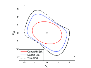
Figure 1: Estimated ROA for isolated and free subsystem $\mathcal{S}_{9}$.

Note that these LFs are computed only once for the network, and stored to be used for real-time control design.

5.2 Controller Design: Test Case

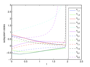
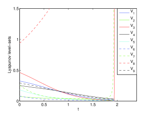
Figure 2: System states (selected) and Lyapunov functions starting from an unstable initial condition, without any control.

Figure 2 shows the evolution of the system state variables (belonging to subsystems $\mathcal{S}_{1}\,,\,\mathcal{S}_{3}\,,\,\mathcal{S}_{4}\,,\,\mathcal{S}_{5}\,,\,\mathcal{S}_{7}$ and $\mathcal{S}_{8}$) and the subsystem LFs, starting from an unstable initial condition. In particular, the state variables belonging to the subsystems $\mathcal{S}_{3}\,,\,\mathcal{S}_{7}$ and $\mathcal{S}_{8}$ ‘escape’ to infinity while other subsystems remain reasonably bounded, over the shown time window.

Algorithm 1 is used to compute distributed stabilizing linear controllers (with $\bar{U}_{i,1}=0~{}\forall i$), satisfying (15). Table 1 lists the results, while the trajectories after applying control are shown in Fig. 3. Interestingly, even though $\mathcal{S}_{3}$ was unbounded without control (Fig. 2), the algorithm finds that there is actually no need for control in $\mathcal{S}_{3}$ provided its neighbors $\mathcal{S}_{2}$ and $\mathcal{S}_{8}$ remain bounded by their initial level-sets (Fig. 3). On the other hand, $\mathcal{S}_{1}$ and $\mathcal{S}_{4}$ apply control, although they were bounded for over $t\!\in\![0,2)$ without control (Fig. 2).

The distributed control design is, however, conservative. For example, the maximum row-sum of the resulting comparison matrix (with control) is only marginally negative (Table 1), while its maximum eigenvalue actually turns out to be $-0.06$.

Table 1: Distributed Control Results

$i$	$\gamma_{i}^{0}$	$\sum_{j=1}^{9}a_{ij}$	$\sum_{j=1}^{9}a_{ij}\gamma_{j}^{0}$	$\bar{U}_{i,2}$	$u_{t,i,2}\left(x_{i,1},\,x_{i,2}\right)$
1	0.33	-0.000	-0.029	0.17	$-0.22\,x_{1,1}-0.10\,x_{1,2}$
2	0.08	-0.140	-0.000	0.00	—
3	0.46	-0.016	-0.005	0.00	—
4	0.25	-0.000	-0.011	0.12	$-0.18\,x_{4,1}-0.08\,x_{4,2}$
5	0.18	-0.048	-0.007	0.00	—
6	0.08	-0.101	-0.000	0.00	—
7	0.26	-0.094	-0.000	0.65	$-0.47\,x_{7,1}-0.89\,x_{7,2}$
8	0.94	-0.000	-0.109	3.88	$-0.56\,x_{8,1}-2.89\,x_{8,2}$
9	0.29	-0.020	-0.005	0.00	—

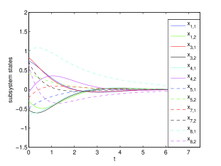
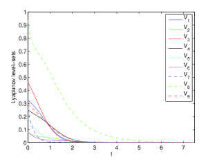
Figure 3: System states and Lyapunov functions with the same initial condition, after application of distributed stabilizing control.

6 Conclusion

The paper presents a distributed control strategy in which agents (subsystems) coordinate with their immediate neighbors to compute optimal local control strategies that exponentially stabilize the full nonlinear network. The proposed algorithm can be easily scalable to very large-scale, sparse, interconnected systems. Future work will explore ways to make the algorithm less conservative. One such way is to use a hierarchical two-level multi-agent control scheme, where the agents exchange some minimal information with a higher-level central agent. The central agent can perform minimal computations such as checking if the comparison matrix is Hurwitz (instead of the diagonally-dominant condition). Higher order polynomials for the subsystem Lyapunov functions could be used for potentially improved control design. It would be interesting to apply the proposed algorithm on some real-world system models, such as a network preserving power system network.

References

- Ames et al. (2014) Ames, A.D., Galloway, K., Sreenath, K., and Grizzle, J.W. (2014). Rapidly exponentially stabilizing control Lyapunov functions and hybrid zero dynamics. Automatic Control, IEEE Transactions on, 59(4), 876–891.
- Anderson and Papachristodoulou (2012) Anderson, J. and Papachristodoulou, A. (2012). A decomposition technique for nonlinear dynamical system analysis. Automatic Control, IEEE Transactions on, 57, 1516–1521.
- Anghel et al. (2013) Anghel, M., Milano, F., and Papachristodoulou, A. (2013). Algorithmic construction of Lyapunov functions for power system stability analysis. Circuits and Systems I: Regular Papers, IEEE Transactions on, 60(9), 2533–2546. 10.1109/TCSI.2013.2246233.
- Araki (1978) Araki, M. (1978). Stability of large-scale nonlinear systems quadratic-order theory of composite-system method using m-matrices. IEEE Transactions on Automatic Control, 23(2), 129 – 142.
- Artstein (1983) Artstein, Z. (1983). Stabilization with relaxed controls. Nonlinear Analysis: Theory, Methods & Applications, 7(11), 1163–1173.
- Bailey (1966) Bailey, F.N. (1966). The application of Lyapunov’s second method to interconnected systems. J. SIAM Control, 3, 443 – 462.
- Beckenbach and Bellman (1961) Beckenbach, E.F. and Bellman, R. (1961). Inequalities. Spring-Verlag, New York/Berlin.
- Bell (1965) Bell, H.E. (1965). Gershgorin’s theorem and the zeros of polynomials. American Mathematical Monthly, 292–295.
- Bellman (1962) Bellman, R. (1962). Vector Lyapunov functions. Journal of the Society for Industrial & Applied Mathematics, Series A: Control, 1(1), 32–34.
- Brauer (1961) Brauer, F. (1961). Global behavior of solutions of ordinary differential equations. Journal of Mathematical Analysis and Applications, 2(1), 145–158.
- Bullo et al. (2009) Bullo, F., Cortés, J., and Martinez, S. (2009). Distributed Control of Robotic Networks. Princeton University Press, Princeton, New Jersey.
- Freeman and Kokotovic (2008) Freeman, R.A. and Kokotovic, P.V. (2008). Robust nonlinear control design: state-space and Lyapunov techniques. Springer Science & Business Media.
- Gershgorin (1931) Gershgorin, S.A. (1931). Uber die abgrenzung der eigenwerte einer matrix. Izv. Akad. Nauk. USSR Otd. Fiz.-Mat. Nauk, 1(6), 749–754.
- Jarvis-Wloszek (2003) Jarvis-Wloszek, Z.W. (2003). Lyapunov Based Analysis and Controller Synthesis for Polynomial Systems using Sum-of-Squares Optimization. Ph.D. thesis, University of California, Berkeley, CA.
- Jocic and Šiljak (1977) Jocic, L. and Šiljak, D. (1977). On decomposition and transient stability of multimachine power systems. Richerche di Automatica, 8(1), 41–57.
- Lasserre (2009) Lasserre, J.B. (2009). Moments, Positive Polynomials and Their Applications, volume 1. World Scientific.
- Lyapunov (1892) Lyapunov, A.M. (1892). The General Problem of the Stability of Motion. Kharkov Math. Soc., Kharkov, Russia.
- Papachristodoulou et al. (2013) Papachristodoulou, A., Anderson, J., Valmorbida, G., Prajna, S., Seiler, P., and Parrilo, P.A. (2013). SOSTOOLS: Sum of squares optimization toolbox for MATLAB. Available from http://www.eng.ox.ac.uk/control/sostools.
- Papachristodoulou and Prajna (2005) Papachristodoulou, A. and Prajna, S. (2005). A tutorial on sum of squares techniques for systems analysis. In Proceedings of the 2005 American Control Conference, 2686–2700.
- Parrilo (2000) Parrilo, P.A. (2000). Structured Semidefinite Programs and Semialgebraic Geometry Methods in Robustness and Optimization. Ph.D. thesis, Caltech, Pasadena, CA.
- Prajna et al. (2005) Prajna, S., Papachristodoulou, A., Seiler, P., and Parrilo, P.A. (2005). Positive Polynomials in Control, chapter SOSTOOLS and Its Control Applications, 273–292. Springer-Verlag, Berlin, Heidelberg.
- Putinar (1993) Putinar, M. (1993). Positive polynomials on compact semi-algebraic sets. Indiana University Mathematics Journal, 42(3), 969–984.
- Slotine et al. (1991) Slotine, J.J.E., Li, W., et al. (1991). Applied Nonlinear Control, volume 199. Prentice-Hall Englewood Cliffs, NJ.
- Sontag (1989) Sontag, E.D. (1989). A ‘universal’ construction of artstein’s theorem on nonlinear stabilization. Systems & control letters, 13(2), 117–123.
- Sturm (1999) Sturm, J.F. (1999). Using SeDuMi 1.02, a MATLAB toolbox for optimization over symmetric cones. Optimization Methods and Software, 11-12, 625–653. Software available at http://fewcal.kub.nl/sturm/software/sedumi.html.
- Tan (2006) Tan, W. (2006). Nonlinear Control Analysis and Synthesis using Sum-of-Squares Programming. Ph.D. thesis, University of California, Berkeley, CA.
- Van der Pol (1926) Van der Pol, B. (1926). On relaxation-oscillations. The London, Edinburgh, and Dublin Philosophical Magazine and Journal of Science, 2(11), 978–992.
- Šiljak (1972) Šiljak, D.D. (1972). Stability of large-scale systems under structural perturbations. Systems, Man and Cybernetics, IEEE Transactions on, SMC-2(5), 657–663. 10.1109/TSMC.1972.4309194.
- Šiljak (1978) Šiljak, D.D. (1978). Large Scale Dynamic Systems: Stability and Structure. System Science and Engineering. North-Holland, New York.
- Weissenberger (1973) Weissenberger, S. (1973). Stability regions of large-scale systems. Automatica, 9(6), 653–663.
- Wloszek et al. (2005) Wloszek, Z.J., Feeley, R., Tan, W., Sun, K., and Packard, A. (2005). Positive Polynomials in Control, chapter Control Applications of Sum of Squares Programming, 3–22. Springer-Verlag, Berlin, Heidelberg.
- Zečević and Šiljak (2010) Zečević, A.I. and Šiljak, D.D. (2010). Control of Complex Systems: Structural Constraints and Uncertainty. Communications and Control Engineering. Springer, New York.
- Zhang et al. (2009) Zhang, W., Abate, A., Hu, J., and Vitus, M.P. (2009). Exponential stabilization of discrete-time switched linear systems. Automatica, 45(11), 2526–2536.