The Magnus expansion and the in-medium similarity renormalization group

Abstract

We present an improved variant of the in-medium similarity renormalization group (IM-SRG) based on the Magnus expansion. In the new formulation, one solves flow equations for the anti-hermitian operator that, upon exponentiation, yields the unitary transformation of the IM-SRG. The resulting flow equations can be solved using a first-order Euler method without any loss of accuracy, resulting in substantial memory savings and modest computational speedups. Since one obtains the unitary transformation directly, the transformation of additional operators beyond the Hamiltonian can be accomplished with little additional cost, in sharp contrast to the standard formulation of the IM-SRG. Ground state calculations of the homogeneous electron gas (HEG) and ¹⁶O nucleus are used as test beds to illustrate the efficacy of the Magnus expansion.

I Introduction

The quest to predict and understand the properties of exotic nuclei starting from the underlying nuclear forces represents a cornerstone of modern nuclear theory. Already for stable nuclei, there are computational and theoretical challenges that make the ab-initio description of nuclear structure quite difficult. Nevertheless, tremendous progress has been made over the past two decades, where it is now possible to perform quasi-exact calculations including three-nucleon interactions of nuclei up through Carbon or so in Quantum Monte Carlo (QMC) and No-Core Shell Model (NCSM) calculations, and $N=Z$ nuclei up through ²⁸Si in lattice effective field theory with Euclidean time projection Lovato et al. (2014); Barrett et al. (2013); Lähde et al. (2014).

Since exact methods scale unfavorably with system size, it is necessary to develop approximate, but systematically improvable methods to extend the reach of ab-initio theory beyond light nuclei. Over the past decade, Coupled Cluster (CC) theory, Self-Consistent Green’s Functions (SCGF), Auxiliary Field Diffusion Monte Carlo (AFDMC), and the In-Medium Similarity Renormalization Group (IM-SRG) have been successfully applied to calculate properties of selected medium mass nuclei and infinite nuclear matter Hagen et al. (2014a); Somá et al. (2014); Carbone et al. (2013); Hergert et al. (2014); Tsukiyama et al. (2011); Roth et al. (2012); Gandolfi et al. (2014). Early applications of these methods were limited primarily to ground state properties of stable nuclei near shell closures with two-nucleon forces only. In recent years, however, substantial progress has been made on including three-nucleon forces Hagen et al. (2007); Somá et al. (2014); Roth et al. (2012); Hergert et al. (2013a), targeting excited states and observables besides energy Ekströ m et al. (2014); Jansen (2013), and moving into the more challenging terrain of open-shell and unstable nuclei Tsukiyama et al. (2012); Jansen et al. (2014); Bogner et al. (2014); Soma et al. (2013); Hergert et al. (2013b).

The IM-SRG is a particularly appealing method due to its flexibility to target ground and excited state properties for closed- and open-shell systems. As discussed in Sec. II, the essence of the IM-SRG is to perform a continuous unitary transformation on the Hamiltonian (and all other observables of interest) to drive it to a diagonal or block-diagonal form. The transformation is implemented by solving a coupled set of flow equations for the matrix elements of the Hamiltonian and any other operators of interest

$$H(s)=U^{\dagger}(s)HU(s)\quad \Leftrightarrow \quad\frac{dH(s)}{ds}=[\eta(s),H(s)]$$

$$O(s)=U^{\dagger}(s)OU(s)\quad \Leftrightarrow \quad\frac{dO(s)}{ds}=[\eta(s),O(s)]\,,$$

where $s$ is a continuous flow parameter, and the choice of the generator $\eta(s)\equiv\frac{dU^{\dagger}}{ds}U$ implicitly defines the transformation $U(s)$. Despite the flexibility to tailor $\eta$ to a wide range of problems and the modest computational scaling with system size, the formulation in Eq. I suffers from the following difficulties:

• The coupled ODEs can become stiff for certain choices of generator and/or for systems with strong correlations.

• The numerical integration of Eq. I requires a high-order ODE solver to accurately preserve the eigenvalues of the evolved Hamiltonian. The use of a high-order solver consumes a large amount of memory since multiple copies of the solution vector (e.g., 15-20 for the predictor-corrector solver of Shampine and Gordon Shampine and Gordon (1975)) need to be stored at each time step.

• For each additional observable of interest, the number of coupled ODEs that need to be solved is roughly doubled, assuming a comparable level of truncation for the evolved operator as the Hamiltonian. Moreover, the flow equations for the additional observable(s) can exacerbate the problems with stiff ODEs, since the time scales for the operator evolution may be very different from those of the Hamiltonian.

In the present paper, we will demonstrate how these difficulties can be circumventedby using the Magnus expansion to recast Eq. I as a flow equation for the operator $\Omega(s)$, where $U(s)=e^{\Omega(s)}$. The unitary operator $U(s)$ is subsequently used to transform the Hamiltonian and any other operators of interest via the Baker-Cambell-Hausdorff (BCH) formula. We will show that in the Magnus expansion formulation, one can use a naive first-order forward Euler method to solve the flow equations for $\Omega(s)$ without any loss of accuracy. This provides a substantial reduction in memory consumption, and allows operators beside the Hamiltonian to be evolved with little additional cost, in sharp contrast to the original formulation of the IM-SRG based on direct integration of Eq. I.

The remainder of the paper is organized as follows: In Section II, we review the basic formalism of the SRG and illustrate how the Magnus expansion can be used to make its numerical implementation more efficient for a schematic model. In Section III, we give some implementation details of our IM-SRG and Magnus expansion calculations of the homogeneous electron gas (HEG) and ¹⁶O nucleus. Results are presented in Section IV, and conclusions are presented in Section V.

II Formalism

II.1 SRG

The similarity renormalization group consists of a continuous sequence of unitary transformations that gradually suppress off-diagonal matrix elements, driving the Hamiltonian towards a band- or block-diagonal form Glazek and Wilson (1993); Wegner (2001); Bogner et al. (2007); Binder et al. (2013). Writing the transformed Hamiltonian as

$$H(s) =U(s)HU^{\dagger}(s)\equiv H^{d}(s)+H^{od}(s),$$ (2)

where $H^{d}(s)$ and $H^{od}(s)$ are the arbitrarily defined “diagonal” and “off-diagonal” parts of the Hamiltonian, the evolution with the continuous flow parameter $s$ is given by

$$\frac{dH(s)}{ds} =[\eta(s),H(s)],$$ (3)

where the $\eta(s)\equiv U(s)dU^{\dagger}(s)/ds$ is the (anti-hermitian) generator of the transformation. The choice of the generator first suggested by Wegner,

$$\eta(s) =[H^{d}(s),H(s)]=[H^{d}(s),H^{od}(s)],$$ (4)

guarantees

$$\frac{d}{ds}Tr\left((H^{od})^{2}\right) =2Tr(\eta^{2})=-2Tr(\eta^{\dagger}\eta)\leq 0,$$ (5)

which demonstrates that the strength of $H^{od}$ decays with increasing $s$Wegner (2001). By analyzing the flow equations in the eigenbasis of $H^{d}(s)$ and defining $H^{d}_{ii}(s)\equiv\epsilon_{i}$, one can show that the Wegner generator gives a super-exponential decay of the off-diagonal matrix elements

$$H^{od}_{ij}(s)\sim e^{-s(\epsilon_{i}-\epsilon_{j})^{2}}H^{od}_{ij}(0)\,.$$ (6)

The SRG evolution with the Wegner generator closely resembles the conventional Wilsonian RG, since matrix elements between widely-separated energy scales are eliminated before moving inwards towards the diagonal. The Wegner generator is numerically very stable, but the different rates of decay for off-diagonal matrix elements can lead to stiff ODEs. To avoid this, two alternative classes of generators are commonly used in nuclear applications. The first alternative was proposed by White in Ref. White (2002)

$$\eta_{ij}(s)=\frac{H^{od}_{ij}(s)}{\epsilon_{i}-\epsilon_{j}}\,,$$ (7)

which leads to a uniform suppression of off-diagonal matrix elements

$$H^{od}_{ij}(s)\sim e^{-s}H^{od}_{ij}(0)\,.$$ (8)

The White generator is numerically very efficient for well-behaved problems, though it can become unstable when the energy denominator in Eq. 7 becomes too small. In Ref. Hergert et al. (2014), the so-called “imaginary time” generator was proposed as a compromise between the White and Wegner generators

$$\eta_{ij}(s)=sign\bigl{(}\epsilon_{i}-\epsilon_{j}\bigr{)}H^{od}_{ij}(s)\,,$$ (9)

where the leading behavior of the off-diagonal matrix elements is

$$H^{od}_{ij}(s)\sim e^{-s|\epsilon_{i}-\epsilon_{j}|}H^{od}_{ij}(0)\,.$$ (10)

In the present paper, all of our IM-SRG calculations were done using the White generator. However, we stress that the computational benefits of the Magnus expansion carry over irrespective of the specific choice of generator.

II.2 In-medium Evolution

Until recently, most SRG applications to nuclear interactions have been carried out in free space to “soften” two- and three-nucleon interactions to be used as input for ab-initio calculations Bogner et al. (2008, 2010); Binder et al. (2013). The free-space evolution is convenient, as it does not have to be performed for each different nucleus or nuclear matter density. However, it is necessary to consistently evolve three-nucleon (and possibly higher) interactions to be able to soften the interactions significantly and maintain approximate $s$-independence of $A\geqslant 3$ observables. The consistent SRG evolution of three-nucleon operators represents a significant technical challenge that has only recently been solved in recent years Jurgenson et al. (2009); Hebeler (2012); Wendt (2013).

An interesting alternative is to perform the SRG evolution in-medium (IM-SRG) for each $A$-body system of interest Bogner et al. (2010); Tsukiyama et al. (2011). Unlike the free-space evolution, the IM-SRG has the appealing feature that one can approximately evolve $3,...,A$-body operators using only two-body machinery by normal-ordering with respect to an $A$-body reference state. Moreover, with a suitable definition of the off-diagonal part of the Hamiltonian to be driven to zero, the IM-SRG can be used as an ab-initio method in and of itself, rather than simply to soften the Hamiltonian as in the free-space SRG.

Starting from a general second-quantized Hamiltonian with two- and three-body interactions,

$$\hat{H} =\sum_{qr}T_{qr}a_{q}^{\dagger}a_{r}+\frac{1}{2!^{2}}\sum_{qrst}V^{(2)}_{qrst}a_{q}^{\dagger}a_{r}^{\dagger}a_{t}a_{s}$$

$$+\frac{1}{3!^{2}}\sum_{qrstuv}V^{(3)}_{qrstuv}a_{q}^{\dagger}a_{r}^{\dagger}a_{s}^{\dagger}a_{v}a_{u}a_{t}+\cdots$$ (11)

all operators can be normal-ordered with respect to a finite-density Fermi vacuum $|\Phi\rangle$ (e.g., the Hartree-Fock ground state), as opposed to the zero-particle vacuum. Wick’s theorem can then be used to exactly write $H$ as

$$H =E+\sum_{qr}f_{qr}:{{a}}^{{\dagger}}_{q}a_{r}:+\frac{1}{4}\sum_{qrst}\Gamma_{qrst}:{{a}}^{{\dagger}}_{q}{{a}}^{{\dagger}}_{r}a_{t}a_{s}:$$

$$\hphantom{=}+\frac{1}{36}\sum_{qrstuv}W_{qrstuv}:{{a}}^{{\dagger}}_{q}{{a}}^{{\dagger}}_{r}{{a}}^{{\dagger}}_{s}a_{v}a_{u}a_{t}:\,,$$ (12)

where strings of normal-ordered operators obey the following relation.

$$\langle{\Phi}|\,{:{{a}}^{{\dagger}}_{q}\ldots a_{r}:}\,|{\Phi}\rangle=0\,,$$ (13)

and the terms in Eq. (II.2) are given by

$$E =\sum_{q}T_{qq}n_{q}\hphantom{=}+\frac{1}{2}\sum_{qr}\!V^{(2)}_{qrqr}n_{q}n_{r}$$

$$\hphantom{=}+\frac{1}{6}\sum_{qrs}V^{(3)}_{qrsqrs}n_{q}n_{r}n_{s}\,,$$ (14)

$$f_{qr} =T_{qr}+\sum_{s}\!V^{(2)}_{qsrs}n_{s}+\frac{1}{2}\sum_{st}V^{(3)}_{qstrst}n_{s}n_{t}\,,$$ (15)

$$\Gamma_{qrst} =\!V^{(2)}_{qrst}+\sum_{u}V^{(3)}_{qrustu}n_{u}\,,$$ (16)

$$W_{qrstuv} =V^{(3)}_{qrstuv}\,.$$ (17)

Here, the initial $n$-body interactions are denoted by $V^{(n)}$, and $n_{q}=\theta(\epsilon_{\rm F}-\epsilon_{q})$ are occupation numbers in the reference state $|\Phi\rangle$, with Fermi energy $\epsilon_{\rm F}$. It is evident that the normal-ordered $0$-, $1$-, and $2$-body terms include contributions from the three-body interaction $V^{(3)}$ through sums over the occupied single-particle states in the reference state $|\Phi\rangle$. Neglecting the residual three-body interaction leads to the normal-ordered two-body approximation (NO2B), which has been shown to be an excellent approximation in many nuclear systems Roth et al. (2012); Binder et al. (2013); Hagen et al. (2007). Truncating the in-medium SRG equations to normal-ordered two-body operators, which we denote by IM-SRG(2), will approximately evolve induced three- and higher-body interactions through the nucleus-dependent 0-, 1-, and 2-body terms.

Using Wick’s theorem to evaluate Eq. 3 with $H(s)=E_{0}(s)+f(s)+\Gamma(s)$ and $\eta(s)=\eta^{(1)}(s)+\eta^{(2)}(s)$ truncated to normal-ordered two-body operators, one obtains the coupled IM-SRG(2) flow equations

$$\frac{d{E}}{d{s}} =\sum_{qr}\eta_{qr}f_{rq}(n_{q}-n_{r})+\frac{1}{2}\sum_{qrst}\eta_{qrst}\Gamma_{stqr}n_{q}n_{r}\bar{n}_{s}\bar{n}_{t}\,,$$ (18)

$$\frac{d{f_{qr}}}{d{s}} =\sum_{s}(1+P_{qr})\eta_{qs}f_{sr}$$

$$\quad+\sum_{st}(n_{s}-n_{t})(\eta_{st}\Gamma_{tqsr}-f_{st}\eta_{tqsr})$$

$$\quad+\sum_{stu}(n_{s}n_{t}\bar{n}_{u}+\bar{n}_{s}\bar{n}_{t}n_{u})(1+P_{qr})\eta_{uqst}\Gamma_{stur}$$ (19)

$$\frac{d{\Gamma_{qrst}}}{d{s}} =\sum_{u}\left\{(1-P_{qr})(\eta_{qu}\Gamma_{urst}-f_{qu}\eta_{urst})\right\}$$

$$\quad-\sum_{u}\left\{(1-P_{st})(\eta_{us}\Gamma_{qrut}-f_{us}\eta_{qrut})\right\}$$

$$\quad+\frac{1}{2}\sum_{uv}(1-n_{u}-n_{v})(\eta_{qruv}\Gamma_{uvst}-\Gamma_{qruv}\eta_{uvst})$$

$$\quad-\sum_{uv}(n_{u}-n_{v})(1-P_{qr})(1-P_{st})\eta_{vrut}\Gamma_{uqvs}\,,$$ (20)

where $\bar{n}_{r}\equiv 1-n_{r}$ and the $s$-dependence has been suppressed for brevity.

Figure 1: Schematic representation of the initial and final Hamiltonians, $H(0)$ and $H(\infty)$, in the many-body Hilbert space spanned by particle-hole excitations of the reference state.

For the calculation of the ground state of a closed-shell system in the IM-SRG(2) approximation, it is simple to identify $H^{\rm od}=\{\Gamma_{abij},f_{ai},+h.c\}$, where $a,b$ denote particle (unoccupied) and $i,j$ hole (occupied) single particle states, as the relevant vertices which connect our chosen reference state $\,|{\Phi}\rangle$ with higher particle-hole excitations, see Fig. 1. By designing a generator to eliminate these terms, one finds that the 0-body term approaches the interacting ground state energy in the limit of large $s$,

$$\lim_{s\rightarrow\infty}E_{0}(s)=\langle\Phi|H(s)|\Phi\rangle=E_{gs}\,.$$ (21)

In the present paper we use the White generator White (2002), though we deviate slightly from recent implementations that use Epstein-Nesbett energy denominators Hergert et al. (2013a), opting for the simpler Møller-Plosset energy denominators

$$\eta =\sum_{ai}\frac{f_{ai}}{f_{a}-f_{i}}:{{a}}^{{\dagger}}_{a}a_{i}:$$

$$+\frac{1}{4}\sum_{abij}\frac{\Gamma_{abij}}{f_{a}+f_{b}-f_{i}-f_{j}}:{{a}}^{{\dagger}}_{a}{{a}}^{{\dagger}}_{b}a_{j}a_{i}:-\text{H.c.}\,,$$ (22)

where $f_{a}=f_{aa}$, etc. The use of Møller-Plosset denominators has minimal impact on the results of ground state IM-SRG(2) calculations, but it has the virtue of revealing the connection to MBPT. In a subsequent work, this connection will be used to develop approximations that go beyond the IM-SRG(2).

II.3 Magnus Expansion

IM-SRG calculations typically use ODE solvers based on high-order Runge-Kutta or predictor-corrector methods to solve Eq. 3. The use of a high-order method is essential as the accumulation of time-step errors will destroy the unitary equivalence between $H(s)$ and $H(0)$, even if no truncations are made in the flow equations. State-of-the-art solvers can require the storage of 15-20 copies of the solution vector in memory, which becomes problematic for large model spaces. The problem is exacerbated if one wants to calculate additional observables, roughly doubling the memory requirements assuming the same NO2B truncation as for the Hamiltonian. Moreover, the additional flow equations for each observable can evolve with rather different timescales than the Hamiltonian, which increases the likelihood of the ODEs becoming stiff.

To bypass these limitations, we now describe an alternative method to solving Eq. (3) using the Magnus expansion Magnus (1954). In the notation of our present problem, our starting point is the differential equation obeyed by the unitary transformation,

$$\frac{dU(s)}{ds}=-\eta(s)U(s)\,,$$ (23)

where $U(0)=1$ and $U^{\dagger}(s)U(s)=U(s)U^{\dagger}(s)=1$. This can be formally integrated and written as the time-ordered exponential

$$U(s) =T_{s}\bigl{\{}e^{-\int_{0}^{s}\eta(s^{\prime})ds^{\prime}}\bigr{\}}$$ (24)

$$\equiv 1-\int_{0}^{s}ds^{\prime}\eta(s^{\prime})+\int_{0}^{s}ds^{\prime}\int_{0}^{s^{\prime}}ds^{\prime\prime}\eta(s^{\prime})\eta(s^{\prime\prime})+\ldots$$

Eq. LABEL:eq:torderexp2 is not very useful in practical calculations since i) there is no guidance on how the series should be truncated, ii) one would need to store $\eta$ for multiple $s$-values, and iii) it is not obvious how to consistently transform the Hamiltonian and other observables in a fully linked, size-extensive manner with the truncated series.

The Magnus expansion is essentially a statement that, given a few technical requirements on $\eta(s)$, a solution of the form

$$U(s)=e^{\Omega(s)}$$ (26)

exists, where $\Omega^{\dagger}(s)=-\Omega(s)$ and $\Omega(0)=0$. In most previous applications of the Magnus expansion, one typically expands $\Omega(s)$ in powers of $\eta(s)$ as

$$\Omega=\sum_{n=1}^{\infty}\Omega_{n}\,.$$ (27)

For issues of convergence and mathematical details, see Refs. Blanes et al. (2009); Fel’dman (1984). Combining this with the formally exact derivative

$$\begin{split}\frac{d\Omega}{ds}=\sum_{k=0}^{\infty}\frac{B_{k}}{k!}ad_{\Omega}^{k}(\eta)\,\\ ad_{\Omega}^{0}(\eta)=\eta\\ ad_{\Omega}^{k}(\eta)=[\Omega,ad_{\Omega}^{k-1}(\eta)]\,,\end{split}$$ (28)

where $B_{k}$ are the Bernoulli numbers and $ad_{\Omega}^{k}(\eta)$ the recursively defined nested commutators, one can obtain explicit expressions for the $\Omega_{n}(s)$,

$$\begin{split}\Omega_{1}(s)&=-\int_{0}^{s}ds_{1}\eta(s_{1})\\ \Omega_{2}(s)&=\frac{1}{2}\int_{0}^{s}ds_{1}\int_{0}^{s_{1}}ds_{2}[\eta(s_{1}),\eta(s_{2})]\\ \vdots\end{split}$$ (29)

As expected, rewriting the time-ordered exponential as a true matrix exponential moves the complications of time ordering into the expression for $\Omega(s)$. The utility of the Magnus expansion lies in the fact that, even if $\Omega$ is truncated to low-orders in $\eta$, the resulting transformation in Eq. 26 using the approximate $\Omega$ is unitary, in contrast to any truncated version of Eq. 24.

For large-scale IM-SRG calculations, the expressions in Eq. 29 are of limited value since they require the storage of $\eta(s)$ over a range of $s$-values. Therefore, in the present work we instead construct $\Omega(s)$ by numerically integrating Eq. 28, subject to certain approximations discussed below. The transformed Hamiltonian, and any other operator of interest, can then be constructed by applying the Baker-Cambell-Hausdorff (BCH) formula,

$$H(s) =e^{\Omega}H\,e^{-\Omega}=\sum_{k=0}^{\infty}\frac{1}{k!}ad_{\Omega}^{k}(H)$$ (30)

$$O(s) =e^{\Omega}O\,e^{-\Omega}=\sum_{k=0}^{\infty}\frac{1}{k!}ad_{\Omega}^{k}(O)\,.$$ (31)

Before discussing how we truncate Eqs. 28 and 30 in practical calculations, it is instructive to study a simple matrix model that can be solved without any truncations. Consider the initial Hamiltonian

$$H=T+V=\begin{pmatrix}1&1\\ 1&-1\end{pmatrix}\,,$$ (32)

where the diagonal “kinetic energy” term is

$$T=\begin{pmatrix}1&0\\ 0&-1\end{pmatrix}\,.$$ (33)

Let us now try to diagonalize $H$ using the Wegner generator $\eta(s)=[T,H(s)]$, solving the SRG equations using the Magnus expansion and by direct integration of Eq. 3. Note that for this choice of initial $H$, both $\eta(s)$ and $\Omega(s)$ are real, antisymmetric matrices throughout the flow

$$\eta(s) =ig_{\eta}(s)\sigma_{2}$$ (34)

$$\Omega(s) =ig_{\Omega}(s)\sigma_{2}\,,$$ (35)

where $\sigma_{2}$ is the Pauli matrix. Consequently, Eq. 28 terminates at the first term and Eq. 30 can be summed up to all orders using the well-known properties of Pauli matrices. Since the large memory footprint of high-order adaptive solvers is the main computational challenge in large-scale SRG calculations, let us instead try to use a naive first-order Euler method to integrate Eqs. 3 and 28. The results are shown in Fig. 2, where we plot $|H_{11}(s)-E_{gs}|$ – which should go to zero at large $s$ – versus $s$ for different Euler step sizes $\delta s$. Unsurprisingly, we see that the direct integration of Eq. 3 accumulates large time-step errors, with the plateaus at large $s$ displaying a strong dependence on the Euler step size. The Magnus solution, on the other hand, converges to a final answer at large $s$ that is independent of step size and agrees with the exact result to within machine precision. The insensitivity to the time step size is due to the fact that while each Euler step in Eq. 28 gives an error of order $\mathcal{O}(\delta s^{2})$, the exponentiated operator at the end of the evolution is still unitary. This is the primary advantage of the Magnus expansion; by reformulating the problem to solve flow equations for $\Omega(s)$ instead of $H(s)$, one can use a simple first-order Euler method and dramatically reduce memory usage. Once $\Omega(s)$ is in hand, the transformation of $H(s)$ and any other observables of interest immediately follows from Eq. 30. In contrast to the direct integration of Eq. I, the dimensionality of the flow equations does not increase when one evolves additional observables.

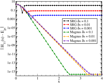
Figure 2: (Color online) $|H_{11}(s)-E_{\rm gs}|$ versus $s$ for different Euler step sizes calculated via direct integration of the SRG flow equation, Eq. 3, and using the Magnus expansion, Eqs. 28 and 30.

II.4 Magnus(2) Approximation

Having illustrated the advantages of the Magnus expansion in a simple model, we would now like to apply it in many-body calculations. Unlike in coupled cluster theory where the BCH formula for the similarity transformed Hamiltonian terminates at finite order, Eqs. 28 and 30 involve an infinite-order series of nested commutators that generate up to $A$-body operators. To make progress, we introduce the Magnus(2) truncation in which all commutators (as well as $\Omega(s),\eta(s)$ and $H(s)$) are truncated to the NO2B level. Even with this approximation, the expressions for $d\Omega/ds$ and $H(s)$ involve an infinite number of terms. However, for both Eqs. 28 and 30 at the NO2B level, we empirically find that the magnitude of terms decreases monotonically in $k$ for all systems studied thus far. Therefore, we numerically truncate Eqs. 28 at the $k^{\rm th}$ term if

$$\biggl{|}\frac{B_{k}\|ad_{\Omega}^{k}(\eta)\|}{k!\|\Omega\|}\biggr{|}<\epsilon_{\rm deriv}\,.$$ (36)

For the truncation of (30), we could use a similar criteria as for the derivative expression. However, since we are interested in the ground-state energy, we use a simpler condition where the series is truncated when the zero-body piece of the $k^{\rm th}$ term falls below some threshold,

$$\biggl{|}\frac{\{ad^{k}_{\Omega}(H)\}_{0b}}{k!}\biggr{|}<\epsilon_{\rm BCH}\,.$$ (37)

In the calculations presented below, we will find that the final results are insensitive to large variations in $\epsilon_{\rm deriv}$ and $\epsilon_{\rm BCH}$, which we take as an a posteriori justification for our truncations.

III Hamiltonians and Implementation

Before presenting the results of IM-SRG(2) and Magnus(2) calculations of the homogeneous electron gas (HEG) and ¹⁶O, we review some details of our implementations for both systems. For the homogeneous electron gas, we perform our calculations for the closed-shell configuration of $N=14$ electrons in a cubic box with periodic boundary conditions. Note that if one is interested in extrapolating to the thermodynamic limit, calculations should be done for a larger closed-shell configurations of $N=38,54,66,\ldots$ electrons, with finite-size corrections for the kinetic and potential energy taken into account. Here we neglect these corrections since our primary purpose is to demonstrate the effectiveness of the Magnus expansion, and the quasi-exact Full Configuration Interaction Quantum Monte Carlo (FCIQMC) results we compare against also neglect these corrections Shepherd et al. (2012). The relevant single particle orbitals are plane waves with quantized momenta

$$\psi_{\mathbb{k}\sigma}(\mathbb{r})=\frac{1}{\sqrt{L^{3}}}e^{i\mathbb{k}\cdot\mathbb{r}}\chi_{\sigma}\,,$$ (38)

where $L^{3}$ is the box volume, $\chi_{\sigma}$ is a spin eigenfunction, and $\mathbb{k}=\frac{2\pi}{L}(n_{x},n_{y},n_{z})$ where $n_{x},n_{y},$ and $n_{z}$ are integers. We follow common practice and use the Wigner-Seitz radius to characterize the density of the HEG,

$$r_{s}=\frac{r_{0}}{a_{0}}\,,$$ (39)

where $a_{0}$ is the Bohr radius and $r_{0}$ is defined in terms of the inverse density as

$$\frac{4}{3}\pi r_{0}^{3}=\frac{L^{3}}{N}\,.$$ (40)

We use a basis set truncation which keeps $M$ single particle states with energy less than some cutoff $E_{c}$, although other choices are possible Hagen et al. (2014b).

In the plane wave basis, the kinetic energy matrix elements are diagonal

$$T_{i,j}=\frac{1}{2}\mathbb{k_{i}}^{2}\delta_{ij}\,,$$ (41)

and the Coulomb matrix elements are given by

$$V_{ijkl}=\frac{1}{L^{3}}\frac{1}{q^{2}}\delta_{\sigma_{i},\sigma_{k}}\delta_{\sigma_{j},\sigma_{l}}\delta_{\mathbb{q},\mathbb{k}_{i}-\mathbb{k}_{k}}\delta_{\mathbb{q},\mathbb{k}_{l}-\mathbb{k}_{j}}.$$ (42)

Note that the $\mathbb{q}=0$ term is omitted due to its cancellation against the inert, uniform positively charged background that is needed to make the system charge neutral Fetter and Walecka (1971). Since we are interested primarily in the correlation energy, we have omitted the Madelung term in all of our calculations.

For the calculations of ¹⁶O, our starting point is the intrinsic nuclear $A$-body Hamiltonian

$$H=\biggl{(}1-\frac{1}{A}\biggr{)}T+T^{(2)}+V^{(2)}\,,$$ (43)

where $T^{(2)}$ is the two-body part of the intrinsic kinetic energy, and we restrict our attention to two-nucleon interactions only. Results are presented for input NN interactions derived from the N³LO (500 MeV) potential of Entem and Machleidt Entem and Machleidt (2003) at several different free-space SRG resolution scales, $\lambda=2.0,2.7$, and $3.0$ fm^-1.

For both systems, the Magnus(2) and IM-SRG(2) calculations start by normal ordering the Hamiltonian with respect to the HF ground state. In the case of the HEG, translational invariance implies the HF orbitals are plane waves. Therefore, the HF reference state is just a Slater determinant comprised of the lowest energy doubly occupied plane wave states for $N=14$ electrons. For ¹⁶O, we must self-consistently solve the Hartree-Fock equations by expanding the unknown HF orbitals in a harmonic oscillator basis truncated to oscillator states obeying $2n+l\leq e_{\rm max}$, where $e_{\rm max}$ is sufficiently large so that the results are approximately independent of the $\hbar\omega$ value of the underlying oscillator basis. For the NN interactions used in the present calculations, a cutoff of $e_{\rm max}=8$ is sufficiently large for most purposes. Once a converged HF ground-state is obtained, the Hamiltonian is normal-ordered w.r.t. to this solution, and the resulting in-medium zero-, one-, and two-body operators serve as the initial values for the Magnus(2) and IM-SRG(2) flow equations. These are subsequently integrated until sufficient decoupling is achieved, as determined by the size of the second-order many-body perturbation theory MBPT(2) contribution of the flowing Hamiltonian $H(s)$ to the ground state energy. We use a threshold of $10^{-6}$ Hartree (MeV) for the HEG (¹⁶O) calculations, respectively, which corresponds to relative changes in the flowing ground-state energy of $10^{-7}$ or less for both systems.

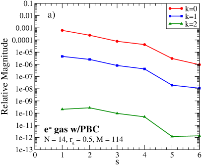
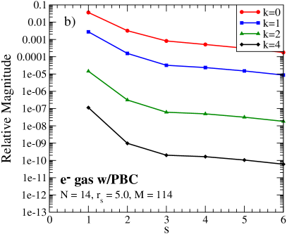
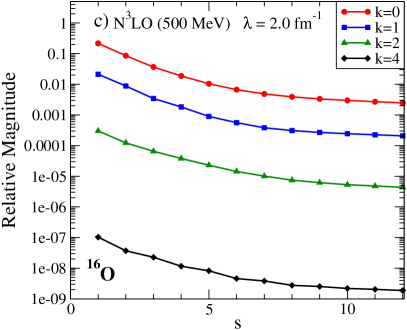
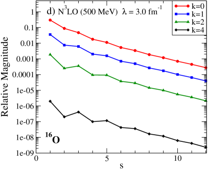
Figure 3: (Color online) Relative importance of the $k^{\rm th}$ term in the Magnus derivative as defined by the lefthand side of Eq. 36 evaluated in the NO2B approximation. The top row is for the homogeneous electron gas at Wigner-Seitz radii of a) $r_{s}=0.5$ and b) $r_{s}=5.0$. The bottom row is for ¹⁶O, starting from the chiral NN potential of Entem and Machleidt Entem and Machleidt (2003), softened by a free-space SRG evolution to (c) $\lambda=2.0$ fm^-1 and (d) $\lambda=3.0$ fm^-1. The electron gas calculations were done for $N=14$ electrons in a periodic box with $M=114$ single particle orbitals. The ¹⁶O calculations were done in an $e_{max}=8$ model space, with $\hbar\omega=24$ MeV for the underlying harmonic oscillator basis.

IV Results

We begin by examining the numerical evidence for truncating Eqs. 28 and 30 by hand. In Figure 3, we plot the lefthand side of Eq. 36 for the HEG (top row) and ¹⁶O (bottom row) as a function of the flow parameter. To assess the role of correlations, the HEG calculations were performed at two different Wigner-Seitz radii, $r_{s}=0.5$ and $r_{s}=5.0$, and the ¹⁶O calculations were done using NN interactions at two different resolution scales, $\lambda=2.0$ fm^-1 and $\lambda=3.0$ fm^-1. For the HEG, the $r_{s}=0.5$ contributions are completely negligible by the $k=2$ term, which is not surprising since the kinetic energy dominates in this weakly correlated high-density regime Fetter and Walecka (1971). Even for the $r_{s}=5.0$ case, where correlations and non-perturbative effects start to become sizable, one finds that the successive terms in Eq. 28 decrease monotonically, though the individual terms are substantially larger than for the $r_{s}=0.5$ case. Analogous results are found for ¹⁶O; the individual terms are larger for the harder $\lambda=3.0$ fm^-1 interaction since the system is more strongly correlated, but they systematically decrease with increasing order $k$.

Figure 4 tells a similar story for the BCH formula, where the lefthand side of Eq. 37 is plotted as a function of the flow parameter. In all cases, we see the importance of successive terms decreases monotonically. Reassuringly, we find that the final results in our calculations are essentially independent of the convergence criteria provided $\epsilon_{{\rm deriv}}\lesssim 10^{-4}$ and $\epsilon_{{\rm BCH}}\lesssim 10^{-4}$, where the latter is in units of Hartree (MeV) for the HEG (¹⁶O) calculations, respectively. For instance, raising both convergence criteria from $10^{-8}$ to $10^{-4}$ changes the ground state energy at the 1 eV ($10^{-7}$ Hartree) level in the ¹⁶O (HEG) calculations, respectively.

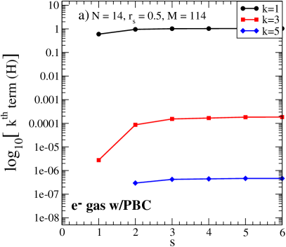
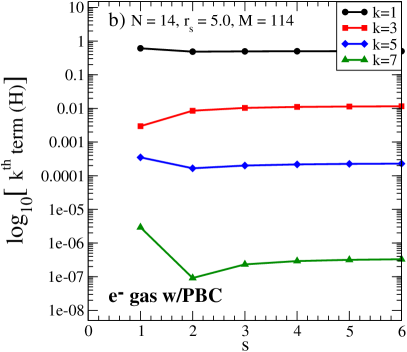
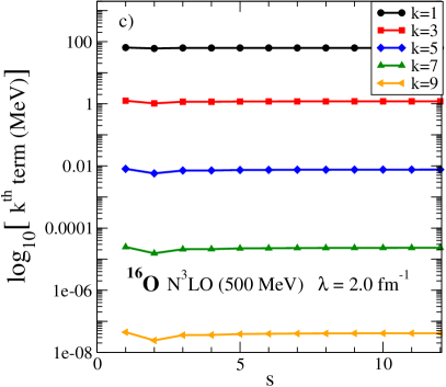
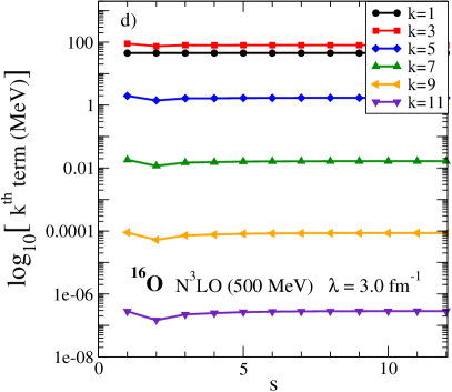
Figure 4: (Color online) Magnitude of the 0-body contributions of the $k^{\rm th}$ term in Eq. 30 evaluated in the NO2B approximation. The top row is for the electron gas at Wigner-Seitz radii of (a) $r_{s}=0.5$ and (b) $r_{s}=5.0$. The bottom row is for ¹⁶O, starting from the chiral NN potential of Entem and Machleidt Entem and Machleidt (2003), softened by a free-space SRG evolution to (c) $\lambda=2.0$ fm^-1 and (d) $\lambda=3.0$ fm^-1. The electron gas calculations were done for $N=14$ electrons in a periodic box with $M=114$ single particle orbitals. The ¹⁶O calculations were done in an $e_{max}=8$ model space, with $\hbar\omega=24$ MeV for the underlying harmonic oscillator basis.

As was illustrated for the toy model in Section II.3, the key advantage of the Magnus expansion is that one can use a first-order Euler method to accurately solve the flow equations. We now demonstrate that the same conclusion holds for realistic IM-SRG calculations. Referring to Figs. 5 and 6, we show the 0-body part of the flowing Hamiltonian $H(s)$ versus the flow parameter for the electron gas and ¹⁶O. The black solid lines denote the results of a standard IM-SRG(2) calculation using the adaptive ODE solver of Shampine and Gordon, while the other curves denote IM-SRG(2) and Magnus(2) calculations using a first-order Euler method with different step sizes $\delta s$. For the electron gas, the exact FCIQMC results Shepherd et al. (2012) are shown for reference. Unsurprisingly, the IM-SRG(2) Euler calculations are very poor, with the various step sizes converging to different large-$s$ limits. The Magnus(2) calculations, on the other hand, converge to the same large-$s$ limit in excellent agreement with the standard IM-SRG(2) results. The insensitivity to step size is due to the fact that the time step errors accumulate in $\Omega(s)$ as opposed to $H(s)$. At the end of the flow, $\Omega(s)$ is still an anti-hermitian operator, and the transformation in Eq. 30 is unitary, up to truncation errors in the NO2B approximation.

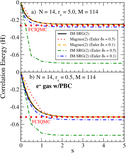
Figure 5: (Color online) Flowing IM-SRG(2) and Magnus(2) HEG correlation energy, $E_{0}(s)-E_{\rm HF}$, for Wigner-Seitz radii of a) $r_{s}=5.0$ and b) $r_{s}=0.5$. The solid black line corresponds to IM-SRG(2) results using an adaptive solver based on the Adams-Bashforth method, while the other lines correspond to Magnus(2) and IM-SRG(2) results using different Euler step sizes. The red circles denote the quasi-exact FCIQMC results of Ref. Shepherd et al. (2012).

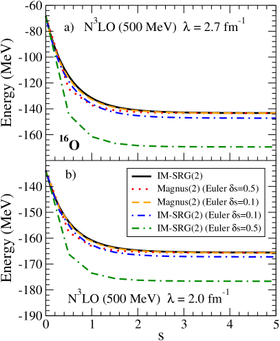
Figure 6: (Color online) Flowing IM-SRG(2) and Magnus(2) ground state energy, $E_{0}(s)$, for ¹⁶O starting from the N³LO NN interaction of Entem and Machleidt Entem and Machleidt (2003) evolved by the free-space SRG to a) $\lambda=2.7$ fm^-1 and $\lambda=2.0$ fm^-1. The solid black line corresponds to IM-SRG(2) results using an adaptive solver based on the Adams-Bashforth method, while the other lines correspond to Magnus(2) and IM-SRG(2) results using different Euler step sizes. The calculations were done in an $e_{max}=8$ model space, with $\hbar\omega=24$ MeV for the underlying harmonic oscillator basis.

Given that the Magnus(2) results are independent of step size over the range considered, one might try to keep increasing the step size to reach the ground state in fewer steps. This unfortunately is not possible, as the flow tends to diverge with too large of a time step. One of the strengths of the SRG approach is that the transformation is adapted as the Hamiltonian is transformed. With too large of a time step, we rob the method of this flexibility and run the risk of applying a “large rotation” of the Hamiltonian that induces large three- and higher-body components. This would not be a problem if we evaluated the BCH and Magnus derivative expressions without approximation; the method would find its way back since the large rotation is still unitary if no truncations are made. However, in the Magnus(2) approximation we make, the neglect of the induced three- and higher-body terms can lead to a lack of convergence. Empirically, we find that this difficulty is avoided by enforcing that at each time step the “off-diagonal” matrix norm $\|H^{\rm od}\|$ is decreasing. This can be implemented by using a simple mid-point integrator algorithm and decreasing the time step if $\|H^{\rm od}\|$ has increased between the first and second half of a step.

As a final demonstration of the utility of the Magnus expansion, we turn to the evolution of operators other than the Hamiltonian. In the conventional approach based on the direct integration of Eq. I, the dimensionality of the flow equations increases with each additional operator to be evolved. In contrast, in the Magnus expansion the dimensionality of the flow equations does not change; the additional computational expense shows up only in the evaluation of the BCH formula for the transformed operator, Eq. 31. For a given operator $O$, we have

$$\langle\Psi_{0}|O|\Psi_{0}\rangle=\lim_{s\rightarrow\infty}\langle\Phi|e^{\Omega(s)}Oe^{-\Omega(s)}|\Phi\rangle\,,$$ (44)

where $|\Phi\rangle$ is the reference state. Therefore, the 0-body piece of the transformed operator approaches the interacting ground state expectation value in the large-$s$ limit.

As a proof-of-principle, we perform a Magnus(2) evolution to evaluate the ground state expectation value of the momentum distribution operator $\hat{n}_{\bf k}\equiv a^{\dagger}_{\bf k}a_{\bf k}$ for the HEG, and the generalized center of mass (COM) Hamiltonian for the ¹⁶O nucleus,

$$H_{\rm cm}(\tilde{\omega})=T_{\rm cm}+\frac{1}{2}mA\tilde{\omega}^{2}R^{2}_{\rm cm}-\frac{3}{2}\hbar\tilde{\omega}\,.$$ (45)

Figure 7 shows the Magnus(2) ground state momentum distribution for a system of $N=14$ electrons in a periodic box for several different Wigner-Seitz radii. Even with the neglect of finite size corrections and the extremely coarse momentum grid due to the small box sizes considered, the qualitative behavior agrees with expectations for the electron gas; correlations become more important at larger $r_{s}$, leading to a stronger depletion of modes with $k<k_{F}$ and smaller discontinuity at the Fermi surface. We note that the Magnus(2) results are in good agreement with the IM-SRG(2) calculations based on Eq. I as well as results generated by the Feynman-Hellman theorem, but at a fraction of the cost. In addition to providing a memory-efficient means for evolving operators beyond the Hamiltonian, Fig. 8 shows that the Magnus(2) approximation gives a small but robust computational speedup for a range of basis sets, even including the additional effort of generating the momentum distributions, which were not computed in the IM-SRG(2) timings.

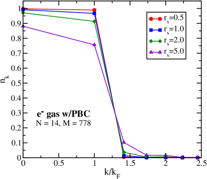
Figure 7: (Color online) (Color online) Electron gas momentum distributions calculated in the Magnus(2) approximation. The calculations were done for $N=14$ electrons in a periodic box with $M=778$ single particle orbitals.

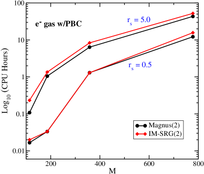
Figure 8: (Color online) Timing for Magnus(2) and IM-SRG(2) HEG calculations as the single particle basis is increased. The two bottom curves are for $r_{s}=.5$ and the top for $r_{s}=5$. For the Magnus(2) timing, this includes the calculations of the momentum distributions.

For our second illustration of operator evolution, we consider the generalized COM Hamiltonian, Eq. 45. In calculations of nuclei, the ground state expectation value of this quantity is useful to diagnose whether approximate solutions of the Schrödinger equation are contaminated by spurious COM motion. Since nuclei are self-bound objects governed by a translationally-invariant Hamiltonian, an exact solution of the Schrödinger equation must factorize into the product of a wave function for the physically relevant intrinsic motion times a wave function for the COM coordinate,

$$|\Psi\rangle=|\psi\rangle_{\rm in}\otimes|\psi\rangle_{\rm cm}\,.$$ (46)

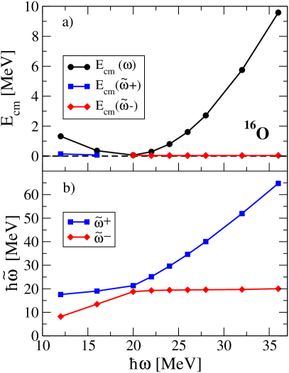
Figure 9: (Color online) (Color online) Center of mass diagnostics for Magnus(2) calculations of ¹⁶O starting from the N³LO NN interaction of Entem and Machleidt Entem and Machleidt (2003) evolved by the free-space SRG to $\lambda=2.0$ fm^-1. See the text for details. The calculations were done in an $e_{\rm max}=9$ model space.

As is well known, there are two strategies to rigorously guarantee this factorization; one can work in a translationally-invariant basis from the outset, or one can work in a so-called full $N\hbar\omega$ model space comprised of all $A$-particle harmonic oscillator Slater determinants with excitations up to and including $N\hbar\omega$. Neither choice is optimal since the former is limited to light nuclei due to the factorial scaling of the required antisymmetrization, while the latter limits the choice of the single particle orbitals to the harmonic oscillator basis and doesn’t carry over to methods that are capable of reaching heavier nuclei, such as coupled cluster theory and the IM-SRG where it is more natural to define the model space via an energy cutoff (e.g., $2n+1\leq e_{\rm max}$) on the single particle states. In the case of calculations with an $e_{\rm max}$ cutoff, there is no analytical guarantee that the COM and intrinsic wave functions factorize.

In Ref. Hagen et al. (2009), Hagen and collaborators gave an ingenious prescription to diagnose whether or not Eq. 46 is satisfied in such calculations. The basic idea is to assume that the factorized COM wave function is a Gaussian, and is therefore the ground state of $H_{\rm cm}(\tilde{\omega})$ with eigenvalue zero. Note that $\tilde{\omega}\neq\omega$ in general, where $\omega$ is the frequency of the underlying oscillator basis. The prescription to find $\tilde{\omega}$ involves solving a quadratic equation

$$\hbar\tilde{\omega}=\hbar\omega+\frac{2}{3}E_{\rm cm}(\omega)\pm\sqrt{\frac{4}{9}(E_{\rm cm}(\omega))^{2}+\frac{4}{3}\hbar\omega E_{\rm cm}(\omega)},$$ (47)

where

$$E_{\rm cm}(\omega) \equiv\langle\Psi|H_{\rm cm}(\omega)|\Psi\rangle$$ (48)

$$=\lim_{s\rightarrow\infty}\langle\Phi|e^{\Omega(s)}H_{\rm cm}(\omega)e^{-\Omega(s)}|\Phi\rangle$$ (49)

$$=\lim_{s\rightarrow\infty}\bigl{\{}e^{\Omega(s)}H_{\rm cm}(\omega)e^{-\Omega(s)}\bigr{\}}_{\rm 0b}\,.$$ (50)

Since there are two roots of Eq. 47, we choose the one that gives a smaller value for $E_{\rm cm}(\tilde{\omega})$. Applying this prescription to our calculations of ¹⁶O, we obtain the results shown in Fig. 9. In the top panel, we see that the expectation value of the COM Hamiltonian $H_{\rm cm}(\omega)$ is approximately zero for $\omega\approx 20$ MeV, but varies parabolically and becomes rather large away from this point. This suggests that if Eq. 46 is satisfied, the frequency of the factorized COM Gaussian should have $\tilde{\omega}\approx 20$ MeV. This is born out in the bottom panel, where the two roots of Eq. 47 are plotted as a function of $\hbar\omega$. Picking the root that minimizes $E_{\rm cm}(\tilde{\omega})$, we find that indeed $\tilde{\omega}\approx 20$ MeV over a wide range of $\omega$, and that $E_{\rm cm}(\tilde{\omega})\approx 0$. Since the excitation energy for the first spurious COM mode is $\hbar\tilde{\omega}\approx 20$ MeV, while $E_{\rm cm}(\tilde{\omega})$ ranges between $0.03$-$0.14$ MeV over the entire range of $\hbar\omega$, we conclude that the factorization of COM/intrinsic motion is satisfied to an excellent approximation.

V Summary and Outlook

In this paper, we have shown how the Magnus expansion can be used to bypass computational limitations arising from the large memory demands of high-order ODE solvers typically used in IM-SRG calculations. The success of the Magnus expansion derives from the fact that by reformulating Eq. I as a flow equation for the operator $\Omega(s)$, where $U(s)=e^{\Omega(s)}$, we are able to use a simple first-order Euler ODE solver without any loss of accuracy, resulting in substantial memory savings and a modest reduction in CPU time. In conventional formulations of the SRG, time step errors accumulate directly in the evolved $H(s)$, necessitating the use of a high-order solver to preserve an acceptable level of accuracy. In the Magnus expansion, even though sizable time step errors accumulate in $\Omega(s)$ with a first-order Euler method, upon exponentiation the transformation is still unitary, and the transformed $H(s)=U^{\dagger}(s)HU(s)$ is unitarily equivalent to the initial Hamiltonian modulo any truncations made (e.g., the NO2B approximation or numerical truncation of the infinite series) in evaluating the BCH formula.

After introducing the basic formalism of the Magnus expansion and illustrating its numerical virtues for a schematic matrix model, we turned to realistic many-body calculations of the homogeneous electron gas (HEG) and ¹⁶O. To make progress, we introduced the Magnus(2) approximation in which all operators ($H(s),\Omega(s),\eta(s)$) and commutators are truncated at the NO2B approximation, and the non-terminating Magnus derivative, Eq. 28, and BCH formula, Eq. 30, are truncated numerically. In all cases studied, our calculations converge to a final answer that is independent of step size and agrees well with IM-SRG(2) calculations using a high-order solver. Moreover, our final results are independent of the precise convergence criteria for truncating Eqs. 28 and 30 provided that $\epsilon_{\rm deriv}\lesssim 10^{-4}$ and $\epsilon_{\rm BCH}\lesssim 10^{-4}$ MeV (Hartree) for the ¹⁶O (HEG) calculations.

The evaluation of observables besides the Hamiltonian poses considerable challenges in the IM-SRG since the evolution of each additional observable roughly doubles the dimensionality of the flow equations. In the Magnus expansion formulation, the evolution of additional operators is trivial since one solves flow equations for the unitary transformation and then constructs the evolved observables by application of the BCH formula. The dimensionality of the flow equations is fixed, regardless of how many additional operators are being evolved. Proof-of-principle operator evolutions were carried out using the Magnus expansion for the momentum distribution in the HEG, and the generalized COM Hamiltonian in ¹⁶O. This opens the door for the ab-initio calculation of a variety of properties (radii, transition matrix elements, response functions, etc.) in addition to energies for medium-mass nuclei.

References

- Lovato et al. (2014) A. Lovato, S. Gandolfi, J. Carlson, S. C. Pieper, and R. Schiavilla, Phys.Rev.Lett. 112, 182502 (2014).
- Barrett et al. (2013) B. R. Barrett, P. Navrátil, and J. P. Vary, Prog.Part.Nucl.Phys. 69, 131 (2013).
- Lähde et al. (2014) T. A. Lähde, E. Epelbaum, H. Krebs, D. Lee, U.-G. Mei\textbetaner, and G. Rupak, Phys. Lett. B732, 110 (2014).
- Hagen et al. (2014a) G. Hagen, T. Papenbrock, M. Hjorth-Jensen, and D. J. Dean, Rep. Prog. Phys. 77, 096302 (2014a).
- Somá et al. (2014) V. Somá, A. Cipollone, C. Barbieri, P. Navrátil, and T. Duguet, Phys.Rev. C89, 061301 (2014).
- Carbone et al. (2013) A. Carbone, A. Polls, and A. Rios, Phys. Rev. C 88, 044302 (2013).
- Hergert et al. (2014) H. Hergert, S. Bogner, T. Morris, S. Binder, A. Calci, et al., Phys.Rev. C90, 041302 (2014).
- Tsukiyama et al. (2011) K. Tsukiyama, S. Bogner, and A. Schwenk, Phys.Rev.Lett. 106, 222502 (2011).
- Roth et al. (2012) R. Roth, S. Binder, K. Vobig, A. Calci, J. Langhammer, and P. Navrátil, Phys. Rev. Lett. 109, 052501 (2012).
- Gandolfi et al. (2014) S. Gandolfi, A. Lovato, J. Carlson, and K. E. Schmidt, Phys. Rev. C90, 061306 (2014).
- Hagen et al. (2007) G. Hagen, T. Papenbrock, D. J. Dean, A. Schwenk, A. Nogga, M. Włoch, and P. Piecuch, Phys. Rev. C 76, 034302 (2007).
- Hergert et al. (2013a) H. Hergert, S. Bogner, S. Binder, A. Calci, J. Langhammer, et al., Phys.Rev. C87, 034307 (2013a).
- Ekströ m et al. (2014) A. Ekströ m, G. Jansen, K. Wendt, G. Hagen, T. Papenbrock, et al., Phys.Rev.Lett. 113, 262504 (2014).
- Jansen (2013) G. R. Jansen, Phys.Rev. C88, 024305 (2013).
- Tsukiyama et al. (2012) K. Tsukiyama, S. Bogner, and A. Schwenk, Phys.Rev. C85, 061304 (2012).
- Jansen et al. (2014) G. Jansen, J. Engel, G. Hagen, P. Navratil, and A. Signoracci, Phys.Rev.Lett. 113, 142502 (2014).
- Bogner et al. (2014) S. Bogner, H. Hergert, J. Holt, A. Schwenk, S. Binder, et al., Phys.Rev.Lett. 113, 142501 (2014).
- Soma et al. (2013) V. Soma, C. Barbieri, and T. Duguet, Phys.Rev. C87, 011303 (2013).
- Hergert et al. (2013b) H. Hergert, S. Binder, A. Calci, J. Langhammer, and R. Roth, Phys.Rev.Lett. 110, 242501 (2013b).
- Shampine and Gordon (1975) L. F. Shampine and M. K. Gordon, Computer solution of ordinary differential equations: the initial value problem (W. H. Freeman, San Francisco, 1975).
- Evangelista (2014) F. A. Evangelista, The Journal of Chemical Physics 141, 054109 (2014).
- Glazek and Wilson (1993) S. D. Glazek and K. G. Wilson, Phys.Rev. D48, 5863 (1993).
- Wegner (2001) F. Wegner, Phys. Rep. 348, 77 (2001).
- Bogner et al. (2007) S. Bogner, R. Furnstahl, and R. Perry, Phys.Rev. C75, 061001 (2007).
- Binder et al. (2013) S. Binder, J. Langhammer, A. Calci, P. Navrátil, and R. Roth, Phys. Rev. C 87, 021303 (2013).
- White (2002) S. R. White, The Journal of Chemical Physics 117, 7472 (2002).
- Bogner et al. (2008) S. Bogner, R. Furnstahl, P. Maris, R. Perry, A. Schwenk, et al., Nucl.Phys. A801, 21 (2008).
- Bogner et al. (2010) S. Bogner, R. Furnstahl, and A. Schwenk, Prog.Part.Nucl.Phys. 65, 94 (2010).
- Jurgenson et al. (2009) E. Jurgenson, P. Navratil, and R. Furnstahl, Phys.Rev.Lett. 103, 082501 (2009).
- Hebeler (2012) K. Hebeler, Phys.Rev. C85, 021002 (2012).
- Wendt (2013) K. A. Wendt, Phys.Rev. C87, 061001 (2013).
- Magnus (1954) W. Magnus, Communications on Pure and Applied Mathematics 7, 649 (1954).
- Blanes et al. (2009) S. Blanes, F. Casas, J. Oteo, and J. Ros, Physics Reports 470, 151 (2009).
- Fel’dman (1984) E. B. Fel’dman, Physics Letters A 104, 479 (1984).
- Shepherd et al. (2012) J. J. Shepherd, G. H. Booth, and A. Alavi, The Journal of Chemical Physics 136, 244101 (2012).
- Hagen et al. (2014b) G. Hagen, T. Papenbrock, A. Ekstr m, K. Wendt, G. Baardsen, et al., Phys.Rev. C89, 014319 (2014b).
- Fetter and Walecka (1971) A. L. Fetter and J. D. Walecka, Quantum theory of many-particle systems, International series in pure and applied physics (McGraw-Hill, San Francisco, 1971).
- Entem and Machleidt (2003) D. Entem and R. Machleidt, Phys.Rev. C68, 041001 (2003).
- Hagen et al. (2009) G. Hagen, T. Papenbrock, and D. J. Dean, Phys. Rev. Lett. 103, 062503 (2009).