Self-assembly of colloidal bands driven by a periodic external field

Abstract

We study the formation of bands of colloidal particles driven by periodic external fields. Using Brownian dynamics, we determine the dependence of the band width on the strength of the particle interactions and on the intensity and periodicity of the field. We also investigate the switching (field-on) dynamics and the relaxation times as a function of the system parameters. The observed scaling relations were analyzed using a simple dynamic density-functional theory of fluids.

I Introduction

The possibility of obtaining materials with enhanced physical properties from the self-assembly of colloidal particles has motivated experimental and theoretical studies over decades Lash et al. (2015); van Blaaderen and Wiltzius (1995); van Blaaderen (2006); Kim et al. (2011). Initially, the focus was on identifying novel phases and constructing the equilibrium phase diagrams, based on the properties of the individual particles (shape, size, and chemistry) Damasceno et al. (2012); Sacanna et al. (2013); Dias et al. (2013a). However, the impressive advance of optical and lithographic techniques opened the possibility of exploring alternative routes as, for example, the use of substrates and interfaces Cadilhe et al. (2007); Araújo et al. (2008); Garbin (2013); Dias et al. (2013b); Cademartiri and Bishop (2015); Araújo et al. (2015), the control of the suspending medium Silvestre et al. (2014) or the assembly under flow Vezirov et al. (2015). More recently, there has been a sustained interest on the self-assembly under the presence of an electromagnetic (EM) field Swan et al. (2014a, b); Cattes et al. (2015); Löwen (2013); Dobnikar et al. (2013). Uniform EM fields couple to the rotational degrees of freedom of magnetic aspherical particles allowing to control their orientation Davies et al. (2014) or fine-tune the strength and directionality of the particle interactions Löwen (2013); Dobnikar et al. (2013); Dillmann et al. (2013). Space-varying periodic fields are employed to impose constraints on the particle position, forming virtual molds that induce spatial periodic patterns Demirörs et al. (2013); Evers et al. (2013); Erb et al. (2009).

Under external constraints, colloidal suspensions are usually driven out of equilibrium and the relaxation towards equilibrium results from the competition of various mechanisms occurring at different length and time scales. Thus, besides the identification of the equilibrium structures and their dependence on the experimental conditions, it is of paramount practical interest to characterize the kinetic pathways towards the desired structures and the timescales involved. Here, we study the prototypical example of field-driven self-assembly of colloidal particles. For simplicity, we consider the formation of colloidal bands driven by a periodic (sinusoidal) electromagnetic field and study how the equilibrium structures and the dynamics towards equilibrium depend on the field strength and periodicity, as well as on the particle interactions. We perform extensive Brownian dynamics simulations and complement the study with a coarse-grained analysis based on the dynamic density-functional theory of fluids (DDFT).

The paper is organized in the following way. In Section II, we present the model and simulation details. The dependence of the stationary state structure and relaxation dynamics on the model parameters is discussed in Section III. Finally, we draw some conclusions in Section IV.

II Model and Simulations 

We consider a two dimensional system of colloidal particles in the overdamped regime. The pairwise particle interactions are described by the repulsive Yukawa potential,

$$V_{ij}(r)=V_{0}\frac{\exp\left(-\alpha r\right)}{r},$$ (1)

where $r=|\vec{r}_{i}-\vec{r}_{j}|$ is the distance between particles $i$ and $j$. $V_{0}$ sets the energy scale and the screening parameter $\alpha$ sets the range of the potential. A characteristic particle radius, $r_{p}$, can be defined as $r_{p}=(2\alpha)^{-1}$, which we set as the unit of length. For simplicity, we consider only repulsive interactions ($V_{0}>0$). To quantify the pairwise interactions we define the integrated parameter $A=\int V_{ij}(\vec{r})d\vec{r}$ expressed in units of $k_{B}Tr^{2}_{p}$. In the numerical simulations we set $\alpha=1/2$ and change $A$ by varying $V_{0}$.

We consider an external field that is constant along the $y$-direction and periodic along the $x$-direction. The particle/field interaction is described by a periodic potential,

$$V_{ext}(x,y)=V_{ext}(x)=V_{E}\sin\left(\kappa x\right),$$ (2)

where $V_{E}$ is the strength of the potential and

$$\kappa=\frac{2\pi P}{L}$$ (3)

is the wave number. $P$ sets the number of minima of the potential in a system of linear length $L$.

We perform Brownian dynamics simulations where the equation of motion of the colloidal particle $i$ is

$$\gamma\frac{d\vec{r}_{i}}{dt}=-\vec{\nabla}_{i}\left[\sum_{j}V_{ij}(r)+V_{ext}(\vec{r}_{i})\right]+\vec{\xi}_{i},\qquad j\neq i$$ (4)

where $\gamma$ is the Stokes friction coefficient and the last term on the right-hand side $\vec{\xi}_{i}(t)$ is the Langevin force mimicking the particle/fluid interaction, which is randomly sampled from a Gaussian distribution of zero mean and second moment $\left\langle\xi_{i}^{k}(t)\xi_{i}^{l}(t^{\prime})\right\rangle=2k_{B}T\gamma\delta_{kl}\delta(t-t^{\prime})$. The indices $k$ and $l$ run over the spatial dimensions, $k_{B}$ is the Boltzmann constant and $T$ the thermostat temperature of the suspending fluid. Thus, the random force is uncorrelated in time and space.

We start our simulations with a uniform (random) distribution of colloidal particles and switch on the field at $t=0$. The simulations were performed inside square boxes of three different linear lengths $L=\{100,120,150\}$, in units of the particle radius. By fixing the density $\rho=0.0696$, we simulate $N=\{696,1000,1560\}$ colloidal particles, respectively.

Hereafter, the strength of the external potential $V_{E}$ is expressed in units of $k_{B}T$ and time is defined in units of the Brownian time $\tau=r^{2}_{p}\gamma(k_{B}T)^{-1}$, which is the time over which a colloidal particle diffuses over a region equivalent to its area. To integrate the stochastic differential equations of motion we followed the scheme proposed by Brańka and HeyesBrańka and Heyes (1999), which consists of a second-order stochastic Runge-Kutta scheme, with a time-step of $\Delta t=10^{-4}\tau$.

III Results 

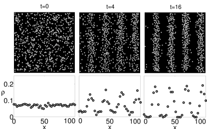
Figure 1: Snapshot of the system for $t=0$, $t=4$ and $t=16$. The plots correspond to the density profiles along the $x$-direction. Under the influence of the external potential the particles organize into bands. The linear length of the system is $L=100$, the interaction parameters are $V_{0}=5$ and $\alpha=1/2$. The strength of the field is $V_{E}=5$ and the number of minima is $P=4$.

In the absence of external fields the spatial distribution of the colloidal particles is homogeneous. When the external field is switched on the particles are dragged towards the closest minimum and self-organize into individual bands around it (see snapshots in Fig. 1). To quantify the spatial arrangement of the colloidal particles we measure the density, $\rho(\vec{r})$, defined as the number of particles per unit area. Given the symmetry of the external field (see Eq. (2)), we focus on the profile of the density along the $x$-direction. Figure 1 shows a snapshot and the density profile for a system with $L=100$ at three different times. The density profile has the symmetry of the external potential. The maxima of the density correspond to the minima of the potential. Similarly, the density vanishes at the maxima of the potential. We run the simulations for $6\times 10^{6}$ timesteps. After this time, the changes in the density profile are within the error bars and thus we consider that the stationary state has been reached. Simulations with different system sizes were preformed and we found no significant finite-size effects.

The collective dynamics and the band structure result from a complex interplay of the particle/fluid, particle/field and particle/particle interactions. Here, we analyze how the final structure and dynamics depend on the model parameters. We start with an analysis of the stationary state and proceed with the study of the dynamics.

III.1 Stationary State

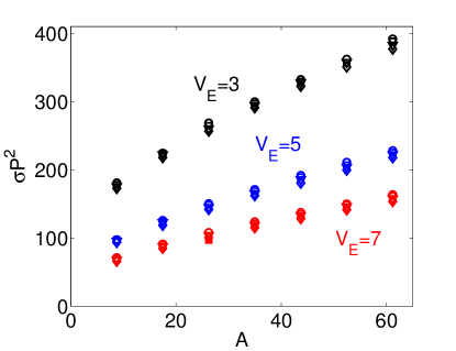
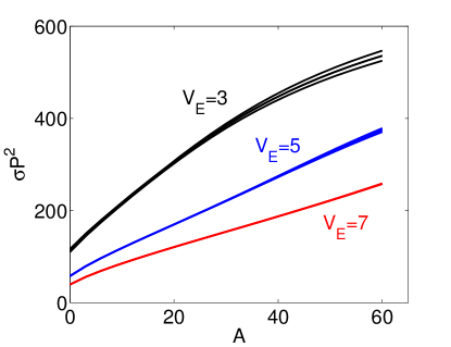
Figure 2: Mean square displacement of the particle position around the potential minima. On the left-hand side are the results obtained from the Brownian dynamics simulations and on the right-hand side those from the DFT calculations. The data is obtained by averaging over $25$ samples rescaled by $P^{-2}$. Black, blue and red represent respectively $V_{E}=\{3,5,7\}$ and the circle, square, triangle and diamond symbols correspond respectively to $P=\{1,2,3,4\}$. The error bars are smaller than the size of the symbols. The particle/particle and particle/field interactions have opposite effects on the final configuration. While the former promotes wider bands the latter favors thinner ones.

III.1.1 Numerical simulations.

We first characterize the stationary state that corresponds to the thermodynamic equilibrium configurations. For $P>L/2$ the average particle/field interaction vanishes, as the wave length of the potential is shorter than the particle diameter. The limit of no external field is then recovered. For $P<L/2$ and strong enough field, particles accumulate around the minima forming a band structure. Thermal noise and particle/particle interaction cause a broadening of the bands, giving them an effective thickness. This thickness is a property of the equilibrium configuration. To quantify it, we measure the mean square displacement of particles around the local minimum

$$\sigma=\langle x_{b}^{2}\rangle-\langle x_{b}\rangle^{2}$$ (5)

where the average is over particles in the same band, i.e., in between two consecutive maxima of the potential. $x_{b}$ is their position relative to the local minimum along the $x$-direction. The average displacement is zero as the distribution of particles is symmetrical with respect to the center of the band (minimum of the potential).

Figure 2 (left panel) shows the dependence of $\sigma$ on the model parameters. One clearly sees that, for a given thermostat temperature, the thickness of the bands results from the competition between particle/field and particle/particle interactions. The particle/field interaction promotes the formation of thin bands. The stronger the field ($V_{E}$) the thinner the band is. By contrast, the particle/particle repulsion tends to homogenize the spatial distribution of the particles and favors wider bands. Consequently, $\sigma$ increases monotonically with $A$. Note that when we rescale $\sigma$ by $P^{2}$ a data collapse is obtained for different $P$ values into a single curve that depends only on $V_{E}$ and $A$. In the next section we perform a density-functional theory (DFT) analysis to study these dependences.

III.1.2 Density-functional theory analysis.

An approximation for the Helmholtz free energy functional can be written as

$$\begin{split}&\mathcal{F}[\rho]=\int k_{B}T\rho(\vec{r})\left[\log\left(\rho(\vec{r})\Lambda^{2}\right)-1\right]d\vec{r}\\ &+\frac{1}{2}\int\int\rho(\vec{r})\rho(\vec{r}^{\prime})V_{pp}(\vec{r}-\vec{r}^{\prime})d\vec{r}^{\prime}d\vec{r}\\ &+\int\rho(\vec{r})V_{ext}(\vec{r})d\vec{r}.\end{split}$$ (6)

On the right-hand side, the first term is the free energy of the ideal gas where $\Lambda$ is the thermal de Broglie wavelength, the second term is the mean-field approximation to the contribution from the interactions and the last term is the external potential contribution. We use the local density approximation (LDA) by setting $\rho(\vec{r}^{\prime})\simeq\rho(\vec{r})$ which is a good assumption if the density is a smooth function of the position.

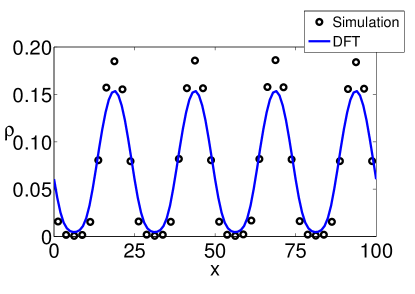
Figure 3: Density profile for $L=100$, $V_{E}=5$, $A=43.71$ and $P=4$. The dots are the numerical results obtained by averaging over $100$ samples and the line is the result of DFT. The theory is in good agreement with the simulations but it underestimates the density at the maxima.

Now we employ the definition of chemical potential, $\mu=\frac{\delta\mathcal{F}[\rho]}{\delta\rho(\vec{r})}$, to obtain

$$k_{B}T\log\left(\rho(\vec{r})\Lambda^{2}\right)+A\rho(\vec{r})+V_{ext}(\vec{r})=\mu.$$ (7)

where $A$ is the interaction parameter defined previously. Rearranging the last equation we find an expression for the density profile

$$\rho(x)=Z\exp[-\beta\left(V_{E}\sin(\kappa x)+A\rho(x)\right)]$$ (8)

where $\beta=(k_{B}T)^{-1}$ and $Z=\Lambda^{-2}e^{\beta\mu}$ is a normalization constant that represents the density of an ideal gas with chemical potential $\mu$. Recall that from the symmetry of the external potential the density is only a function of the $x$-coordinate. To solve this equation we impose an additional constraint $N=\int\rho(\vec{r})d\vec{r}$ arising from the conservation of the total number of particles.

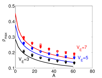
Figure 4: Maximum density of the profile. Each data point is an average over 25 samples and the lines are the DFT results. Black, blue and red represent respectively $V_{E}=\{3,5,7\}$ and the circle, square, triangle and diamond symbols correspond respectively to $P=\{1,2,3,4\}$. The error bars are smaller than the size of the symbols. Note that the density does not depend on $P$. The deviation of the theoretical curves from the simulation results increases particle interactions increase. The effect of $A$ and $V_{E}$ on the maximal density is opposite to their effect on the mean square displacement.

Figure 3 shows the density profile obtained from numerical simulation and DFT for the same set of parameters. The DFT results deviate from the simulation only at the maximal and minimal densitities. The maximal density is underestimated and the minimal is slightly overestimated. We evaluated how this deviation depends on the model parameters. Figure 4 shows the dependence on $A$ of the maximal density $\rho_{max}$, defined as the density in the center of the band, for different values of $V_{E}$ and $P$. We find that, while the deviation of the DFT calculation from the simulation increases slightly with $A$ it does not vary significantly with $V_{E}$ and $P$. This also leads to theoretical values of the mean square displacement $\sigma$, which are larger than those obtained by simulation. However, as shown in Fig. 2 (right panel) one recovers the same qualitative dependence on the model parameters and the values of $\sigma$ are of the same order of magnitude.

Since the density profile is symmetric with respect to the center of the band, the mean square displacement is given by,

$$\sigma=L\int_{-\frac{L}{2P}}^{\frac{L}{2P}}x^{2}\rho^{*}(x)dx.$$ (9)

where $\rho^{*}(x)=\rho(x)N^{-1}_{b}$ is the probability density function for particles in the band and $N_{b}=L\int_{-\frac{L}{2P}}^{\frac{L}{2P}}\rho(x)dx$. The $L$ outside of the integral accounts for the integration of the domain along the $y$-direction. Assuming that $\rho(x)$ is constant and $N_{b}=N/P$,

$$\sigma=\frac{L^{2}}{12P^{2}}\ \ .$$ (10)

Thus, $\sigma\sim P^{-2}$ as observed both from the simulations and the DFT analysis. Note that the maximal density (in Fig. 4) does not depend on $P$. From Eq. (8) we also conclude that, near the minima, the external potential and the interaction terms have different signs. Consequently, $V_{E}$ and $A$ have opposite effects on $\sigma$, as observed in the simulations and DFT calculations, see Fig. 2.

By taking the logarithm of Eq. (8) we obtain

$$\log(\rho(x))+\beta A\rho(x)=log(Z)-\beta V_{E}sin(\kappa x).$$ (11)

The dependence of the first term of the left-hand side on the density can be neglected with respect to the second term in two limiting cases: for strong particle/particle interactions or high enough densities. In the former, the strong particle/particle repulsion hinders the formation of bands and homogenizes the density. The external potential acts as a perturbation to the uniform distribution of particles, which is sinusoidal in space and linear on $V_{E}$. The contributions from the external potential and particle interactions are given by $\rho(x)$ which means that the dependence of the mean square displavement on the strength of the potential intensity is the same in both limits, as seen in Fig. 5(a) and (b). For weak particle interactions the curves are linear when the strength of the potential is also small. But as the particle/particle interaction increases, the potential intensity where the dependence deviates from linear also increases. Note that the curve for $A=0$ corresponds to the ideal gas where the dependence of $\rho(x)$ on the strength of the potential is exponential as expected from Eq. (8). For $V_{E}=0$ the density is uniform and the value of $\sigma$ is given by Eq. (10) and is the same for all curves.

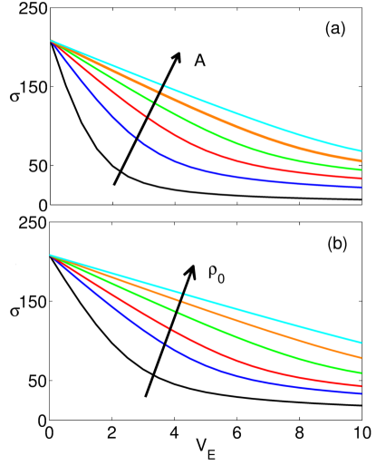
Figure 5: DFT results for the mean square displacement for $P=2$. The lines in (a) are for $A=\{0,20,40,60,80,100\}$ and the lines in (b) are for different initial densities $\rho_{0}=\{2.50,6.96,10.0,15.0,20.0,25.0\}\times 10^{-2}$. For strong inter-particle interactions and weak external potentials the dependence is linear in $V_{E}$. The linear dependence is also observed at high densities.

III.2 Relaxation Dynamics

III.2.1 Numerical simulations.

We analyze now the relaxation towards the stationary state shown in Fig. 1. Namely, we investigate how the relaxation time depends on the model parameters.

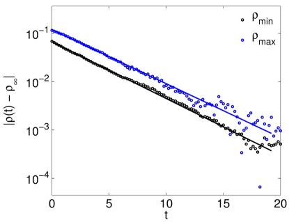
Figure 6: Evolution of the maximal and minimal densities. The relaxation into the stationary state is exponential. The scattered data are the numerical results and the lines the exponential fitting. The results shown are averages over $100$. The parameters are $L=100$, $V_{E}=5$, $A=43.71$ and $P=4$.

We start with a uniform spatial distribution of particles, $\rho(x)=\rho_{0}$. As the external potential is switched on the colloidal particles move accordingly and regions of high density of colloids are formed (bands). For a systematic analysis, we focus on the evolution of the positions of the minima, $\rho_{min}$, corresponding to the potential maxima, and the positions of maxima, $\rho_{max}$, corresponding to the potential minima. Figure 6 shows the convergence of these densities to their value in the stationary state, $\rho_{\infty}$, for a particular set of parameters. One clearly sees an exponential decay in time.

We define the relaxation time $\tau^{relax}$ as the inverse of the slopes of the evolution curves. Figures 7 and 8 show that the dependence on the model parameters is different for the minima and the maxima suggesting that the underlying relaxation mechanisms are different. In general, strong potentials favor short relaxation times while the dependence on the particle/particle interaction is not straightforward. Also, data collapse is observed when we rescale $\tau$ with $P^{2}$. We will now use DDFT to shed light on these findings.

III.2.2 Dynamic density-functional theory analysis.

If we consider that the system evolves adiabatically, the evolution equation of the local density can be written directly from the equilibrium Helmholtz free energy functional Marconi and Tarazona (1999); Rauscher (2010),

$$\gamma\frac{\partial\rho(\vec{r},t)}{\partial t}=\vec{\nabla}.\left[\rho(\vec{r},t)\vec{\nabla}\frac{\delta\mathcal{F}[\rho(\vec{r},t)]}{\delta\rho(\vec{r},t)}\right].$$ (12)

Using the functional defined in Eq. (6), we obtain a diffusion equation for the density,

$$\gamma\frac{\partial\rho}{\partial t}=\vec{\nabla}.\left[A\rho\vec{\nabla}\rho+V_{E}\kappa cos(\kappa x)\rho\right]+k_{B}T\nabla^{2}\rho\ \ ,$$ (13)

where the first and last terms are related to the particle/particle and particle/fluid interactions, respectively. They tend to smooth out any spatial variation of the density. The middle term is related to the particle/field interaction and promotes the formation of bands. Note that, when one applies $\vec{\nabla}.$ to the first term one gets $A\rho\nabla^{2}\rho$, a non-linear diffusion term where the coefficient increases with the density. It is the interplay of the thermostat temperature, external potential and particle/particle interactions that controls the kinetics of relaxation and defines the relaxation time towards the stationary state. A similar diffusion equation can also be obtained from the Fokker-Planck formalism Zapperi et al. (2001).

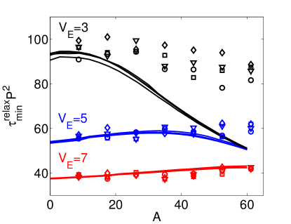
Figure 7: Relaxation time of the minimal density. The scattered data are the simulation results and the solid lines the ones from the DDFT calculations. Black, blue and red represent respectively $V_{E}=\{3,5,7\}$ and the circle, square, triangle and diamond symbols correspond respectively to $P=\{1,2,3,4\}$. The simulation results are averages over $45$ samples for $V_{E}=3$ and $25$ samples in the other cases. The relaxation time does not vary monotonically with the interaction strength. It exhibits a maximum that depends on the balance between $A$ and $V_{E}$. The relaxation time is proportional to $P^{-2}$.

We focus on the maximal and minimal densities where $\vec{\nabla}\rho=0$. Let us assume that $\nabla^{2}\rho=\rho_{2}$ is constant in time at these points. At the minimum $\rho_{2}\geq 0$ and at the maximum $\rho_{2}\leq 0$. By solving Eq. (13) we get

$$\rho_{\begin{subarray}{c}min\\ max\end{subarray}}(t)=-\frac{k_{B}T\rho_{2}}{A\rho_{2}\mp V_{E}\kappa^{2}}+K_{1}\exp\left[\frac{A\rho_{2}\mp V_{E}\kappa^{2}}{\gamma}t\right],$$ (14)

where the expression with the minus sign is for the density at the minimum and the plus sign for the density at the maximum. By fixing the initial density it is possible to calculate the constant

$$K_{1}=\frac{N}{L^{2}}+\frac{k_{B}T\rho_{2}}{A\rho_{2}\mp V_{E}\kappa^{2}}.$$ (15)

If we define the characteristic relaxation time as

$$\rho(t)-\rho_{\infty}\sim e^{-t/\tau^{relax}}$$ (16)

where $\rho_{\infty}$ is the density at the given point at equilibrium, we arrive at the following expression

$$\tau^{relax}_{\begin{subarray}{c}min\\ max\end{subarray}}=-\frac{\gamma}{A\rho_{2}\mp V_{E}\kappa^{2}}.$$ (17)

In the region of parameters where $\nabla^{2}\rho=const$ the relaxation time is inversely proportional to $A$ and $V_{E}$. The friction coefficient also plays a role on the dynamics and the relaxation time is a monotonic increasing function of the viscosity. Replacing $\kappa$ using Eq. (3) we conclude that $\tau^{relax}\sim P^{-2}$. The relaxation time decreases with the number of bands as, on average, particles have to travel a shorter distance to reach the nearest potential minimum. Eq. (13) is solved numerically using first order finite elements in the 2D square domain with periodic boundary conditions com . Figures 7 and 8 show the relaxation time of the minimal and maximal densities, respectively. They collapse for $P^{-2}$ but the inverse proportionality is only observed for high $A$ which is where our approximation holds.

The theoretical results underestimate the relaxation time by comparison with the data from the Brownian dynamics simulations, consistent with the fact that DDFT overestimates the diffusion coefficient Marconi and Tarazona (1999). The deviation is greater at low $V_{E}$ and high $A$, when the particle/particle interactions dominate the dynamics. Recall that the term for particle/particle interaction in Eq. (6) is the only approximate term.

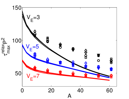
Figure 8: Relaxation time of the maximal density. The scattered data are the numerical results and the solid lines the ones from the DDFT calculations. Black, blue and red represent respectively $V_{E}=\{3,5,7\}$ and the circle, square, triangle and diamond symbols correspond respectively to $P=\{1,2,3,4\}$. The simulation results are averages over $45$ samples for $V_{E}=3$ and $25$ samples in the other cases. For strong interparticle interactions the relaxation time depends weakly on the external potential.

Note that the relaxation time is always positive. For the minimal density the curvature $\rho_{2}$ is typically small and the external potential term dominates. For the maximal density the curvature is negative and the particle/particle interaction term dominates over the external potential. In the minimum the particles try to escape and so the external potential is the relevant interaction leading to a decrease in the density. However, the process is still influenced by the presence of neighboring particles and the relaxation time increases with $A$ at low $A$, Fig. 7. For strong interparticle repulsions there is a broadening of the bands; the particles will then travel shorter distances to reach their equilibrium positions, decreasing $\tau^{relax}$ at the minimal density. By contrast, for the maximal density the repulsions strongly affect the dynamics.

The relaxation times obtained from the simulations and the theory coincide for strong potentials as the effect of the interparticle interactions is irrelevant. When $V_{E}$ decreases the particle/particle repulsion becomes relevant and the LDA approximation leads to increasing deviations from the simulation results. Equation (17) suggests that for high enough values of $A$ the relaxation times do not depend on $V_{E}$ and $P$ and converge to the same value in line with the results shown in Figs. 7 and 8. For lower $A$ at the maxima, where the particles are compressed, equilibrium takes longer to be reached.

IV Conclusions 

We studied the dependence of the structure and relaxation dynamics of the equilibrium state of a colloidal suspension on the external potential and the interpaticle interactions. The analysis based on density-functional theory was found to be in good agreement with the results from Brownian dynamics simulations.

In the stationary state the system exhibits a band-like structure. The thickness of the bands measured in terms of the mean square displacement, $\sigma$, decreases with the strength of the potential, which leads in turn to higher densities around the external potential minima. We also showed that $\sigma$ scales as $P^{-2}$, where $P$ is the number of bands. In the limit of weak external potentials, $\sigma$ increases linearly with the potential strength, $V_{E}$.

The relaxation towards the stationary extreme densities is exponential but the relaxation times are different. The system takes longer to reach equilibrium at the density maxima except when the external potential becomes significant weak in which case the relaxation time does not depend on the position. At the density maxima $\tau^{relax}$ decreases when both $V_{E}$ and $A$ increase but at the density minima it displays a more complex behavior and there is a maximum relaxation time that depends on the balance between $V_{E}$ and $A$.

Electromagnetic fields are used in the laboratory to promote the formation of a variety of colloidal structures. Our results quantify the relaxation times and the equilibrium structures of simple colloidal systems, which exhibit a rich behaviour that may be controlled in a straightforward manner.

V Acknowledgements

We acknowledge fruitful discussions with D. de las Heras and C. Dias, as well as financial support from the Portuguese Foundation for Science and Technology (FCT) under Contracts nos. EXCL/FIS-NAN/0083/2012, UID/FIS/00618/2013, and IF/00255/2013.

References

- Lash et al. (2015) M. H. Lash, M. V. Fedorchak, J. J. McCarthy, and S. R. Little, Soft Matter 11, 5597 (2015).
- van Blaaderen and Wiltzius (1995) A. van Blaaderen and P. Wiltzius, Science 270, 1177 (1995).
- van Blaaderen (2006) A. van Blaaderen, Nature 439, 545 (2006).
- Kim et al. (2011) S.-H. Kim, S. Y. Lee, and S.-M. Yang, NPG Asia Mater 3, 25 (2011).
- Damasceno et al. (2012) P. F. Damasceno, M. Engel, and S. C. Glotzer, Science 337, 453 (2012).
- Sacanna et al. (2013) S. Sacanna, D. J. Pine, and G.-R. Yi, Soft Matter 9, 8096 (2013).
- Dias et al. (2013a) C. S. Dias, N. A. M. Araujo, and M. M. Telo da Gama, Soft Matter 9, 5616 (2013a).
- Cadilhe et al. (2007) A. Cadilhe, N. A. M. Araújo, and V. Privman, Journal of Physics: Condensed Matter 19, 065124 (2007).
- Araújo et al. (2008) N. A. M. Araújo, A. Cadilhe, and V. Privman, Phys. Rev. E 77, 031603 (2008).
- Garbin (2013) V. Garbin, Phys. Today 66, 68 (2013).
- Dias et al. (2013b) C. S. Dias, N. A. M. Araújo, and M. M. Telo da Gama, Phys. Rev. E 87, 032308 (2013b).
- Cademartiri and Bishop (2015) L. Cademartiri and K. J. M. Bishop, Nat Mater 14, 2 (2015).
- Araújo et al. (2015) N. A. M. Araújo, C. S. Dias, and M. M. T. da Gama, Journal of Physics: Condensed Matter 27, 194123 (2015).
- Silvestre et al. (2014) N. M. Silvestre, Q. Liu, B. Senyuk, I. I. Smalyukh, and M. Tasinkevych, Phys. Rev. Lett. 112, 225501 (2014).
- Vezirov et al. (2015) T. A. Vezirov, S. Gerloff, and S. H. L. Klapp, Soft Matter 11, 406 (2015).
- Swan et al. (2014a) J. W. Swan, J. L. Bauer, Y. Liu, and E. M. Furst, Soft Matter 10, 1102 (2014a).
- Swan et al. (2014b) J. W. Swan, J. L. Bauer, Y. Liu, and E. M. Furst, Soft Matter 10, 1102 (2014b).
- Cattes et al. (2015) S. M. Cattes, S. H. L. Klapp, and M. Schoen, Phys. Rev. E 91, 052127 (2015).
- Löwen (2013) H. Löwen, The European Physical Journal Special Topics 222, 2727 (2013).
- Dobnikar et al. (2013) J. Dobnikar, A. Snezhko, and A. Yethiraj, Soft Matter 9, 3693 (2013).
- Davies et al. (2014) G. B. Davies, T. Krüger, P. V. Coveney, J. Harting, and F. Bresme, Advanced Materials 26, 6715 (2014).
- Dillmann et al. (2013) P. Dillmann, G. Maret, and P. Keim, The European Physical Journal Special Topics 222, 2941 (2013).
- Demirörs et al. (2013) A. F. Demirörs, P. P. Pillai, B. Kowalczyk, and B. A. Grzybowski, Nature 503, 99 (2013).
- Evers et al. (2013) F. Evers, R. Hanes, C. Zunke, R. Capellmann, J. Bewerunge, C. Dalle-Ferrier, M. Jenkins, I. Ladadwa, A. Heuer, R. Castañeda Priego, and S. Egelhaaf, The European Physical Journal Special Topics 222, 2995 (2013).
- Erb et al. (2009) R. M. Erb, H. S. Son, B. Samanta, V. M. Rotello, and B. B. Yellen, Nature 457, 999 (2009).
- Brańka and Heyes (1999) A. C. Brańka and D. M. Heyes, Phys. Rev. E 60, 2381 (1999).
- Marconi and Tarazona (1999) U. M. B. Marconi and P. Tarazona, The Journal of Chemical Physics 110, 8032 (1999).
- Rauscher (2010) M. Rauscher, Journal of Physics: Condensed Matter 22, 364109 (2010).
- Zapperi et al. (2001) S. Zapperi, A. A. Moreira, and J. S. Andrade, Phys. Rev. Lett. 86, 3622 (2001).
- (30) “The COMSOL Multiphysics software is used to implement the FEM.” .