Convergence of a Linearly Transformed Particle Method for Aggregation Equations

Martin Campos Pinto CNRS, UMR 7598, Laboratoire Jacques-Louis Lions, F-75005, Paris, France
Sorbonne Universités, UPMC Univ Paris 06, UMR 7598, Laboratoire Jacques-Louis Lions, F-75005, Paris, France
campos@ann.jussieu.fr
José A. Carrillo Department of Mathematics, Imperial College London, SW7 2AZ, United Kingdom carrillo@imperial.ac.uk Frédérique Charles Sorbonne Universités, UPMC Univ Paris 06, UMR 7598, Laboratoire Jacques-Louis Lions, F-75005, Paris, France
CNRS, UMR 7598, Laboratoire Jacques-Louis Lions, F-75005, Paris, France
charles@ann.jussieu.fr
 and  Young-Pil Choi Department of Mathematics, Imperial College London, SW7 2AZ, United Kingdom young-pil.choi@imperial.ac.uk
Abstract.

We study a linearly transformed particle method for the aggregation equation with smooth or singular interaction forces. For the smooth interaction forces, we provide convergence estimates in $L^{1}$ and $L^{\infty}$ norms depending on the regularity of the initial data. Moreover, we give convergence estimates in bounded Lipschitz distance for measure valued solutions. For singular interaction forces, we establish the convergence of the error between the approximated and exact flows up to the existence time of the solutions in $L^{1}\cap L^{p}$ norm.

Key words and phrases:
Aggregation equations, linearly transformed particle method, smooth and singular interaction potentials
2010 Mathematics Subject Classification:
65M12, 35R09, 35Q82, 35Q92, 35Q35, 82C22

1. Introduction

In this work, we are interested in showing the convergence of approximated particle schemes to the Cauchy problem for the so-called aggregation equation. This equation determines the evolution of a probability density $\rho(t,x)$ defined by

(1.1) $$\left\{\begin{array}[]{ll}\partial_{t}\rho(t,x)+\nabla\cdot(\rho u)(t,x)=0,\quad x\in\mathbb{R}^{d},\quad t>0,&\vspace{.2cm}\\ u(t,x)=-(\nabla W*\rho(t))(x),\quad x\in\mathbb{R}^{d},\quad t>0,&\vspace{.2cm}\\ \rho(0,x)=\rho^{0}(x)\geq 0,\quad x\in\mathbb{R}^{d}.&\end{array}\right.$$

Here, $-\nabla W(x-y)$ measures the interaction force that an infinitesimal particle located at $y\in\mathbb{R}^{d}$ will exert on a particle located at $x\in\mathbb{R}^{d}$. As a result, we will call $W$ the interaction potential. Since the total mass is preserved, without loss of generality, we assume

$$\int_{\mathbb{R}^{d}}\rho(t,x)\,dx=\int_{\mathbb{R}^{d}}\rho^{0}(x)\,dx=1\qquad\forall t\geq 0.$$

The microscopic dynamics of $\mathcal{N}$ particles $X_{i}$, $i=1,\dots,\mathcal{N}$, interacting through the potential $W$ are given by

(1.2) $$\dot{X}_{i}=-\sum_{j\neq i}m_{j}\;\nabla W(X_{i}-X_{j})\,,\qquad i=1,\dots,\mathcal{N}\,,$$

where the inertia term is assumed to be negligible compared to friction [45, 46]. The macroscopic dynamics (1.1) consists of a continuity equation where the velocity field is given by $u(t,x)=-(\nabla W*\rho(t))(x)$, which is the mean-field limit of the microscopic system when $\mathcal{N}\to\infty$ under certain conditions on the potential [32, 37, 18, 20].

Equation (1.1) has attracted lots of attention in the recent years for three reasons: its gradient flow structure [43, 26, 49, 1, 27], the blow-up dynamics for fully attractive potentials [7, 20, 9, 25], and the rich variety of steady states and their bifurcations both at the discrete (1.2) and the continuous (1.1) level of descriptions [35, 36, 6, 47, 22, 21, 9, 2, 3, 50, 51, 4, 15, 19]. Furthermore, these systems are ubiquitous in mathematical modelling appearing in granular media models [5, 43], swarming models for animal collective behavior [33, 42, 24], equilibrium states for self-assembly and molecules [34, 48, 52, 38], and mean-field games in socioeconomics [31, 11] among others.

We will focus the rest of the introduction on the well-posedness of the continuous equation (1.1) and the numerical methods proposed for its approximation. The equation (1.1) has the formal structure of being a gradient flow of a functional in the set of probability measures. Indeed, defining the interaction energy as

$$\mathcal{F}[\mu]:=\frac{1}{2}\int_{\mathbb{R}^{d}}\int_{\mathbb{R}^{d}}W(x-y)\,d\mu(x)\,d\mu(y)$$

for any probability measure $\mu$, we find $u=-\nabla\frac{\delta\mathcal{F}}{\delta\mu}$ where $\frac{\delta\mathcal{F}}{\delta\mu}$ is the formal variation of the functional $\mathcal{F}[\mu]$. This observation leads to a natural formal Lyapunov functional for the solutions of equation (1.1). In fact, we expect solutions to satisfy the identity

$$\frac{d}{dt}\mathcal{F}[\rho(t)]=-\int_{\mathbb{R}^{d}}|\nabla W\ast\rho(t)|^{2}\rho(t)\,dx$$

for all $t\geq 0$. This structure can be rendered fully rigorous for $C^{1}$-potentials [1] and it allows for mildly singular potentials at the origin [20, 21, 25] provided the interaction potential has some convexity property called $\lambda$-convexity.

On the other hand, global in time unique weak measure solutions can be constructed for any probability measure as initial data under suitable smoothness assumptions on the interaction potential. In this work, whenever we refer to smooth potentials, we mean that the interaction potential satisfies $\nabla W\in\mathcal{W}^{1,\infty}(\mathbb{R}^{d})$. For smooth potentials, the approach introduced by Dobrushin for the Vlasov equation [32] using the bounded Lipschitz distance between probability measures, see [37, 18, 14] for further details, gives a well-posedness theory of weak measure solutions.

However, many of the interesting features related to blow-up dynamics and stationary states happen for potentials that are singular at the origin. Typical examples to bear in mind are combinations of repulsive attractive power-law potentials of the form $W(x)=\tfrac{|x|^{a}}{a}-\tfrac{|x|^{b}}{b}$ with $-d\leq b<a$ and the convention $\tfrac{|x|^{0}}{0}=\log|x|$, or fully attractive potentials $W(x)=\tfrac{|x|^{a}}{a}$ with $a>-d$, suitably cut-off at infinity. In this work, whenever we refer to singular potentials we mean that the interaction potential is not smooth but satisfies

$$|\nabla W(x)|\leq\frac{C}{|x|^{\alpha}}\quad\textrm{and}\quad|D^{2}W(x)|\leq\frac{C}{|x|^{1+\alpha}}\quad\mbox{with}\quad-1<\alpha<d-1$$

for some constant $C>0$, and in addition we assume that $\nabla W$ is bounded away from the origin if $\alpha<0$. These conditions allow for singularities at the origin up to Newtonian but not including it. In particular, our singular potentials are such that $\nabla W\in\mathcal{W}^{1,q}_{\rm loc}(\mathbb{R}^{d})$ with a range depending on $\alpha$: $1\leq q<\frac{d}{\alpha+1}$. Note that the power-law potentials satisfy locally the conditions of being a singular potential in the range $2-d<b<2$ for repulsive-attractive and in the range $2-d<a<2$ for fully attractive. The various well-posedness theories for measure solutions fail as soon as the potential becomes singular at the origin. However, weak solutions in Lebesgue spaces can be obtained. A local-in-time well-posedness theory was obtained in [10, 18] for initial data in $(L^{1}\cap L^{p})(\mathbb{R}^{d})$ with $p=q^{\prime}$ the conjugate exponent of $q$, and in [7, 9] a local-in-time well-posedness theory for initial data in $(L^{1}\cap L^{\infty})(\mathbb{R}^{d})$ was developed for singularities up to and including a Newtonian singularity at the origin, corresponding to $\alpha=d-1$. In this work, we will use the setting introduced in [18]. The Newtonian case is very specific because of the relation between the divergence of the velocity field and the density becomes local.

Under the above assumptions of either smooth or singular potentials, the proofs of the global-in-time well-posedness of weak measure solutions and the local-in-time well-posedness of weak solutions for initial data in $(L^{1}\cap L^{p})(\mathbb{R}^{d})$ spaces are essentially based on the fact that the velocity field is regular enough to have meaningful characteristics. It is proved in [32, 37, 10, 18] that the velocity field of the constructed solutions is continuous in time and Lipschitz continuous in space. Then, the flow map $\Phi_{t}(x)$, defined by the unique solution of the characteristic system

$$\left\{\begin{aligned} &\frac{dX}{dt}(t)=u(t,X(t)),\\ &X(s)=x,\end{aligned}\right.$$

is a diffeomorphism for all times $t\geq 0$. In all cases, the solution built in [32, 37, 10, 18] is obtained by characteristics and given by $\rho(t)=\Phi_{t}\#\rho^{0}$. Here, $\mathcal{T}\#\mu$ denotes the push-forward of a measure through a measurable map $\mathcal{T}:\mathbb{R}^{d}\longrightarrow\mathbb{R}^{d}$ defined as $\mathcal{T}\#\mu[K]:=\mu[\mathcal{T}^{-1}(K)]$ for all Borel sets $K\subset\mathbb{R}^{d}$, or equivalently

$$\int_{\mathbb{R}^{d}}\varphi\,d(\mathcal{T}\#\mu)=\int_{\mathbb{R}^{d}}(\varphi\circ\mathcal{T})\,d\mu\qquad\mbox{for all }\varphi\in C_{b}(\mathbb{R}^{d})\,.$$

A very interesting question is the rigorous derivation of the continuum description (1.1) starting from the microscopic dynamics (1.2) for both regular and singular potentials. This is the so-called mean-field limit problem. The mean-field limit results contain as a by-product convergence results for the classical particle method. More precisely, proving that (1.1) is the mean-field limit of the system (1.2) as $\mathcal{N}\to\infty$ is equivalent to show that the empirical measure

$$\mu_{\mathcal{N}}(t)=\frac{1}{\mathcal{N}}\sum_{i=1}^{\mathcal{N}}\delta_{X_{i}(t)}$$

converges weakly in measure sense to the solution of (1.1) provided that this weak convergence holds initially. Even if the particle method is proved to be convergent of order $\frac{1}{\mathcal{N}}$, the convergence error is only controlled in the bounded Lipschitz or Wasserstein-type distances between measures [32, 37, 18, 20].

Vortex-blob methods, originally introduced for the 2D Euler equations for incompressible fluids, see [44] and the references therein, have also been adapted recently to the aggregation equation [8] with fixed shapes, where the approximate densities are shown to converge with arbitrary orders but only in negative Sobolev norms.Particle methods were also used in plasma physics for the Vlasov-Poisson system [30], where they are usually called smooth Particle In Cell (PIC) methods.

In the Linearly Transform Particle (LTP) method, introduced by Campos Pinto in [12] following an idea of Cohen and Perthame [29], particles are pushed on to discrete times according to an approximation of the exact flow as in standard particle methods. Moreover, particles have their own shape, which is transformed in the discrete evolution in order to better approach the local flow using a linearization of the exact flow. To our knowledge the LTP method has only been used for a linear transport equation [29] or for a Vlasov-Poisson system [13] involving measure-preserving characteristic flows. The technical difficulties posed by the deformation of the flows in our present case have been overcome by detailed estimates of the Jacobian matrices and determinants. These estimates have allowed us to control the error on the densities via the errors of the flows to finally obtain the convergence results. Certain Sobolev regularity is needed on the initial data to obtain convergence of the LTP method in Lebesgue spaces for both smooth and singular potentials. However, a general result of convergence for weak measure solutions is obtained in an appropriate distance for measures.

Let us finally mention that other numerical methods have been proposed in the literature for the aggregation equation. In [16], the authors proposed a finite volume scheme which is shown to be energy preserving, i.e., it keeps the property that the energy functional is dissipated along the semidiscrete flow. Finite volume and finite difference schemes have been shown to be convergent to weak measure solutions of the aggregation equations for mildly singular potentials in [41, 25].

In this work, we extend the LTP method to the aggregation equation seen as one of the most important representatives of a class of nonlinear continuity equations with non divergence free velocity fields in any dimensions. We start by summarizing the basic ideas of the numerical LTP method in Section 2 together with the preliminaries and notations used in this work. Section 3 is devoted to give convergence results for smooth potentials in Lebesgue spaces. Depending on the regularity of the initial data, we will be able for smooth potentials to control errors in $L^{1}$ and $L^{\infty}$. For initial data just being a probability measure, we will show in Section 4 the convergence in bounded Lipschitz distance. In the case of singular potentials, we will control in Section 5 the error upto the existence time of the solution of (1.1) in $L^{1}$ and $L^{p}$ with $p$ suitably chosen. We finally show in Section 6 the performance of this method in one dimension validating the numerical implementation with explicit solutions and making use of it to study certain not well-known qualitative features of the evolution of (1.1) with several smooth and singular potentials.

2. Preliminaries

2.1. Basic properties of the exact flow

In the setting of our main results, the velocity field of the exact solution to (1.1) is always continuous in $t$ and Lipschitz continuous in $x$. The solution of the characteristic system

$$\left\{\begin{aligned} &\frac{dX}{dt}(t)=u(t,X(t))\\ &X(s)=x,\end{aligned}\right.$$

is well-defined and it has unique global in time solutions for all initial data $x\in\mathbb{R}^{d}$. Moreover, the general solution of the characteristic system is a diffeomorphism in $\mathbb{R}^{d}$. The general flow map will be denoted by $F^{s,t}(x)$ for all $t,s\in\mathbb{R}$ and $x\in\mathbb{R}^{d}$.

As discussed in the introduction, the solutions to (1.1) can always be expressed as $\rho(t)=F^{0,t}\#\rho^{0}$ or equivalently as

$$\rho(t,x)=\rho^{0}\left(F^{t,0}(x)\right)j^{t,0}(x)\quad\textrm{with}\quad j^{t,0}(x)=\det(J^{t,0}(x)),\quad J^{t,0}(x)=DF^{t,0}(x)\,.$$

The flow map satisfies

(2.1) $$F^{s,t}(x)=x+\int_{s}^{t}u(\tau,F^{s,\tau}(x))d\tau=x-\int_{s}^{t}(\nabla W*\rho(\tau))(F^{s,\tau}(x))d\tau,$$

and the Jacobian matrix and its determinant satisfy the differential equations

(2.2) $$\frac{d}{dt}J^{s,t}(x)=Du(t,F^{s,t}(x))J^{s,t}(x)\quad\mbox{and}\quad\frac{d}{dt}j^{s,t}(x)=\nabla\cdot u(t,F^{s,t}(x))j^{s,t}(x).$$

Using $u(\tau,y)=-(\nabla W*\rho(\tau))(y)$, this yields

$\displaystyle J^{s,t}(x)-I_{d}$ $\displaystyle=\int_{s}^{t}\!Du(\tau,F^{s,\tau}(x))J^{s,\tau}(x)d\tau$
(2.3) $\displaystyle=-\int_{s}^{t}\!(D^{2}W*\rho(\tau))(F^{s,\tau}(x))J^{s,\tau}(x)d\tau$

and

$\displaystyle j^{s,t}(x)$ $\displaystyle=\exp\left(-\int_{s}^{t}\nabla\cdot u(\tau,F^{s,\tau}(x)d\tau\right)$
(2.4) $\displaystyle=\exp\left(-\int_{s}^{t}(\Delta_{x}W*\rho(\tau))(F^{s,\tau}(x))d\tau\right).$

Estimates are then easily derived when $u\in L^{\infty}(0,\infty;\mathcal{W}^{1,\infty}(\mathbb{R}^{d}))$. We will write $L:=\sup_{t\in[0,\infty)}\|u(t,\cdot)\|_{\mathcal{W}^{1,\infty}}$. For instance, using (2.2) and $J^{s,s}(x)=I_{d}$ we find

(2.5) $$\sup_{x\in\mathbb{R}^{d}}\lvert J^{s,t}(x)\rvert\leq\exp\left(CL\lvert t-s\rvert\right),$$

and in particular the characteristic flow is Lipschitz (relative to any norm in $\mathbb{R}^{d}$),

(2.6) $$|F^{s,t}|_{Lip}\leq\exp\left(CL\lvert t-s\rvert\right).$$

Furthermore, we derive from (2.3) and (2.5) that

(2.7) $$\sup_{x\in\mathbb{R}^{d}}\lvert I_{d}-J^{s,t}(x)\rvert\leq(t-s)\exp\left(CL\lvert t-s\rvert\right)$$

and using (2.4) we also find

(2.8) $$\exp\left(-CL\lvert t-s\rvert\right)\leq j^{s,t}(x)\leq\exp\left(CL\lvert t-s\rvert\right)\quad\text{ for }\quad x\in\mathbb{R}^{d}$$

and

(2.9) $$\|j^{s,t}-1\|_{L^{\infty}}\leq CL|t-s|\exp\left(CL(t-s)\right).$$

Let us remark that the previous estimates (2.5)-(2.9) can also be obtained in a time interval $[0,T]$ for locally Lipschitz velocity fields $u\in L^{\infty}(0,T;\mathcal{W}^{1,\infty}(\mathbb{R}^{d}))$ for some $T>0$, with constant $L_{T}:=\sup_{t\in[0,T]}\|u(t,\cdot)\|_{\mathcal{W}^{1,\infty}}$. These estimates will be used in Section 5, where the dependence on T of the Lipschitz constant will be omitted for the sake of simplicity.

2.2. Linearly Transformed Particles

As in standard particle methods, the density $\rho$ is represented with weighted macro-particles, and as in smooth particle methods, particles have here a finite and smooth shape. Thus, we approximate the initial density $\rho^{0}$ on a Cartesian grid of size $h>0$ by

(2.10) $$\rho_{h}^{0}(x)=\sum_{k\in\mathbb{Z}^{d}}\omega_{k}\varphi_{h,k}^{0}(x)$$

with particle shapes obtained by scaling and translating a reference function, i.e.,

(2.11) $$\varphi_{h,k}^{0}(x)=\frac{1}{h^{d}}\varphi\left(\frac{x-x_{k}^{0}}{h}\right),\qquad x_{k}^{0}=kh.$$

Here the reference shape is assumed to have a compact support $\operatorname{supp}(\varphi)\subset B(0,R_{o})$, be bounded and satisfy

$$\sum_{k\in\mathbb{Z}^{d}}\varphi(x-k)=1\quad\text{for $x\in\mathbb{R}^{d}$}\qquad\text{ and }\qquad\int_{\mathbb{R}^{d}}\varphi=1.$$

In this work we will require that the shape functions are Lipschitz, and we can either consider for the reference shape the tensor-product hat function

(2.12) $$\varphi(x)=\prod_{1\leq i\leq d}\max(1-|x_{i}|,0).$$

or the B3-spline

(2.13) $$\varphi(x)=\frac{1}{6}\left\{\begin{array}[]{cc}\left(2-|x|\right)^{3}&\textrm{if }1\leq|x|<2,\\ \displaystyle 4-6x^{2}+3|x|^{3}&\textrm{if }0\leq|x|<1,\\ 0&\textrm{otherwise.}\end{array}\right.$$

As for the weights $\omega_{k}=\omega_{k}(h,\rho^{0})$, they are usually defined as

(2.14) $$\omega_{k}=\int_{x_{k}^{0}+\left[-\frac{h}{2},\frac{h}{2}\right]^{d}}\rho^{0}(x)dx,$$

however this will not be sufficient to prove the convergence of our particle scheme without additional smoothness assumptions on the initial density $\rho^{0}$. Indeed, using standard arguments (see e.g. [12, 28]) based on the fact that the approximation $\rho^{0}\mapsto\rho^{0}_{h}=\sum_{k\in\mathbb{Z}^{d}}\omega_{k}\varphi_{h,k}^{0}$ is local, bounded in any $L^{p}$ space and preserves the affine functions, one easily verifies the following estimate.

Proposition 1.

If $\rho^{0}_{h}$ is initialized as in (2.10) with weights and shape function given by (2.14) and (2.11), respectively, then we have

(2.15) $$\lVert\rho^{0}-\rho^{0}_{h}\rVert_{L^{p}}\leq Ch^{s}\lVert\rho^{0}\rVert_{\mathcal{W}^{s,p}}$$

for $s\in\{0,1,2\}$, $1\leq p\leq\infty$ and a constant $C$ independent of $\rho^{0}$.

In our analysis we will need second-order estimates which are then available for $\rho^{0}\in\mathcal{W}^{2,p}(\mathbb{R}^{d})$. However, if we allow negative weights then second-order estimates are also available in a dual norm, as follows. Consider weights defined as

(2.16) $$\omega_{k}=\int_{\mathbb{R}^{d}}\tilde{\varphi}_{h,k}^{0}(x)\rho^{0}(x)dx$$

with integration kernels bi-orthogonal to the shape functions in the sense that

(2.17) $$\int_{\mathbb{R}^{d}}\varphi_{h,k}^{0}\tilde{\varphi}_{h,k^{\prime}}^{0}=\delta_{k,k^{\prime}}$$

holds with $\delta_{k,k^{\prime}}$ the Kronecker symbol. Similar to the shape functions, they can be obtained by scaling and translating a reference $\tilde{\varphi}$ (assumed again compactly supported, bounded and satisfying (2.2)) with a different normalization, namely

(2.18) $$\tilde{\varphi}_{h,k}^{0}(x)=\tilde{\varphi}\left(\frac{x-x_{k}^{0}}{h}\right).$$

For instance if $\varphi$ is the above tensor-product hat function (2.12) then for the integration kernel we may take $\tilde{\varphi}(x)=\prod_{i\leq d}\big{(}\frac{3}{2}{\mathbbm{1}}_{[-\frac{1}{2},\frac{1}{2}]}-\tfrac{1}{2}{\mathbbm{1}}_{[-1,-\frac{1}{2}]\cup[\frac{1}{2},1]}\big{)}(x_{i}),$ see Figure 1.

Refer to caption
Figure 1. A piecewise affine shape function and its bi-orthogonal kernel (dotted line). Both functions vanish outside $[-1,1]$.

Notice that estimate (2.15) still holds with these weights. Now, from the duality (2.17) we can derive a convenient second-order estimate which only relies on the first-order smoothness of $\rho^{0}$. It is expressed in the dual norm

$$\displaystyle\lVert w\rVert_{\mathcal{W}^{-1,p}}:=\sup_{v\in\mathcal{W}^{1,q}(\mathbb{R}^{d})}\langle w,v\rangle/\lVert v\rVert_{\mathcal{W}^{1,q}}\,,$$

where $q$ is the conjugate exponent of $p$ and $\langle w,v\rangle$ is the duality pair that coincides with the integral of the product $wv$ as soon as the latter is integrable.

Proposition 2.

If $\rho^{0}_{h}$ is initialized as in (2.10) with shape functions and weights satisfying properties (2.11)-(2.2) and (2.16)-(2.18), we have

(2.19) $$\lVert\rho^{0}-\rho^{0}_{h}\rVert_{\mathcal{W}^{-1,p}}\leq Ch^{2}\lVert\rho^{0}\rVert_{\mathcal{W}^{1,p}}$$

for $1\leq p\leq\infty$, with a constant $C$ independent of $h$.

Proof.

It follows from the duality relation (2.17) that $\langle\rho^{0}-\rho^{0}_{h},\tilde{\varphi}_{h,k}^{0}\rangle=0$ for all $k$. In particular, given $v\in\mathcal{W}^{1,\infty}(\mathbb{R}^{d})$ we have

$$\langle\rho^{0}-\rho^{0}_{h},v\rangle=\langle\rho^{0}-\rho^{0}_{h},v-\tilde{v}_{h}\rangle$$

with $\tilde{v}_{h}:=\sum_{k\in\mathbb{Z}^{d}}\langle v,\varphi_{h,k}^{0}\rangle\tilde{\varphi}_{h,k}^{0}$ and standard arguments show that the approximation $v\mapsto\tilde{v}_{h}$ satisfies an error estimate similar to (2.15) for $s=1$. Using the Hölder inequality this gives

$$\langle\rho^{0}-\rho^{0}_{h},v\rangle\leq\lVert\rho^{0}-\rho^{0}_{h}\rVert_{L^{p}}\lVert v-\tilde{v}_{h}\rVert_{L^{q}}\leq Ch^{2}\lVert\rho^{0}\rVert_{\mathcal{W}^{1,p}}\lVert v\rVert_{\mathcal{W}^{1,q}}$$

and the proof is completed due to the definition of the $\mathcal{W}^{-1,p}(\mathbb{R}^{d})$ norm. ∎

We observe that both the above initializations yield

(2.20) $$\sup_{k\in\mathbb{Z}^{d}}\lvert\omega_{k}\rvert\leq Ch^{d/q}\|\rho^{0}\|_{L^{p}}\qquad\text{ where }\qquad\tfrac{1}{q}+\tfrac{1}{p}=1\,,$$

and since the shape functions are assumed to be non-negative, (2.2) gives

(2.21) $$\|\rho_{h}^{0}\|_{L^{1}}\leq\sum_{k\in\mathbb{Z}^{d}}\lvert\omega_{k}\rvert\leq C\|\rho^{0}\|_{L^{1}}\leq C\,,$$

with a constant depending only on $\tilde{\varphi}$.

We now describe the LTP method. As mentioned in the introduction, compared to standard particle methods, the LTP method follows the shape of smooth particles. Therefore we need to track not only the particle positions but also their deformations given by the Jacobian matrices. Given discrete trajectories $x^{n}_{k}$ approximating the exact ones $F^{0,t_{n}}(x^{0}_{k})$ on the discrete times

$$t_{n}:=n\Delta t,\qquad n=0,1,\ldots,N:=T/\Delta t,$$

and non singular approximations $J^{n}_{k}$ of the forward Jacobian matrices $J^{t_{n},t_{n+1}}(x^{n}_{k})$, the particle shapes $\varphi^{n+1}_{h,k}$ are recursively defined as the push-forward of $\varphi^{n}_{h,k}$ along the affine flow

(2.22) $$F_{h,k}^{n}:\,x\mapsto x_{k}^{n+1}+J_{k}^{n}(x-x_{k}^{n})\,,$$

which approximates the exact flow $F^{t_{n},t_{n+1}}$ around $x_{k}^{n}$. Here $x_{k}^{n+1}$ can also be seen as an approximation to $F^{t_{n},t_{n+1}}(x_{k}^{n})$, as will be specified below. In short, we define

$$\varphi^{n+1}_{h,k}:=F_{h,k}^{n}\#\varphi^{n}_{h,k}=\frac{1}{j_{k}^{n}}\varphi^{n}_{h,k}\circ(F_{h,k}^{n})^{-1}\,,$$

where $j_{k}^{n}:=\det(J_{k}^{n})>0$. Starting from $\varphi^{0}_{h,k}$ defined as in (2.11), this gives particles of the form

(2.23) $$\varphi_{h,k}^{n}(x):=\frac{1}{h_{k}^{n}}\varphi\left(\frac{D_{k}^{n}(x-x_{k}^{n})}{h}\right)\,,$$

where the deformation matrix $D_{k}^{n}$ and the particle volume $h_{k}^{n}$ are defined by

(2.24) $$\begin{cases}D_{k}^{n+1}:=D_{k}^{n}\left(J_{k}^{n}\right)^{-1}\\ h_{k}^{n+1}:=j_{k}^{n}h_{k}^{n}=\det(J_{k}^{n})h_{k}^{n}\end{cases}\text{ with }\quad\begin{cases}D_{k}^{0}:=I_{d}\\ h_{k}^{0}:=h^{d}\end{cases}\,.$$

It follows from the above process that $D_{k}^{n}$ is an approximation to the backward Jacobian matrix $J^{t_{n},0}(x^{n}_{k})$, whereas $h_{k}^{n}$ approximates the elementary volume $h^{d}$ multiplied by the Jacobian determinant of the forward flow $F^{0,t_{n}}$ at $x^{0}_{k}$. Moreover, the particle shape $\varphi_{h,k}^{n}$ is the push-forward of $\varphi^{0}_{h,k}$ along the integrated flow

(2.25) $$\overline{F}_{h,k}^{n}:=F^{n-1}_{h,k}\circ\cdots\circ F^{0}_{h,k}:x\mapsto x^{n}_{k}+\overline{J}^{n}_{k}(x-x^{0}_{k})\quad\text{ where }\quad\overline{J}^{n}_{k}:=(D^{n}_{k})^{-1}$$

which can be seen as a linearization of $F^{0,t_{n}}$ around $x^{0}_{k}$ (for $n=0$ we set $\overline{F}_{h,k}^{0}=I$ since $D^{0}_{k}=I_{d}$). Indeed, it follows from the above definitions that

(2.26) $$\varphi_{h,k}^{n}=\overline{F}_{h,k}^{n}\#\varphi^{0}_{h,k}\,,$$

and we easily verify that

$$h_{k}^{n}=h^{d}\det(J_{h,k}^{n-1})\,\cdots\,\det(J_{h,k}^{0})=\frac{h^{d}}{\det(D_{h,k}^{n})}\approx h^{d}\det(J^{0,t_{n}}(x^{0}_{k})).$$

Finally, the LTP approximation of the density at time $t_{n}$ is defined as

(2.27) $$\rho_{h}^{n}(x):=\sum_{k\in\mathbb{Z}^{d}}\omega_{k}\varphi_{h,k}^{n}(x)$$

with weights $\omega_{k}$ constant in time and computed as in (2.14) or (2.16). According to (2.26), we have $\int\varphi^{n}_{h,k}=\int\varphi_{h,k}^{0}=\int\varphi$, and thus the conservation of mass ($\int\rho_{h}^{n}=\int\rho_{h}^{0}$) holds at the discrete level. Moreover, using the fact that the particle shapes are non-negative, we find as in (2.21)

(2.28) $$\|\rho_{h}^{n}\|_{L^{1}}\leq\sum_{k\in\mathbb{Z}^{d}}\lVert\omega_{k}\varphi^{n}_{h,k}\rVert_{L^{1}}=\sum_{k\in\mathbb{Z}^{d}}\lvert\omega_{k}\rvert\leq C\|\rho^{0}\|_{L^{1}}=C,\qquad n\geq 0.$$

2.3. Approximated Jacobian matrices and particle positions

To complete the description of the numerical method (2.23)-(2.24), (2.27), we are left to specify how to compute the particle center $x^{n+1}_{k}$ and the discrete Jacobian matrix $J^{n}_{k}$ involved in the affine flow (2.22). Before doing so we observe that if the matrices $D^{2}W(x)$ and $D^{2}W(y)$ commute for all $x$ and $y$, then the exact solution to the ODE (2.2) takes an exponential form. However, in the general case the matrix $J^{t_{n},t_{n+1}}(x)$ is not equal to

(2.29) $$\tilde{J}^{t_{n},t_{n+1}}(x):=\exp\left(-\int_{t_{n}}^{t_{n+1}}(D^{2}W*\rho(\tau))(F^{t_{n},\tau}(x))d\tau\right)$$

but the difference is small, as shown next.

Proposition 3.

If $u\in L^{\infty}(0,T;\mathcal{W}^{1,\infty}(\mathbb{R}^{d}))$, then we have

$$\lvert\tilde{J}^{t_{n},t_{n+1}}(x)-J^{t_{n},t_{n+1}}(x)\rvert\leq C(\Delta t)^{2}\quad\text{ for }\quad x\in\mathbb{R}^{d},$$

with a constant $C$ independent of $n\leq N-1$ and $\Delta t$.

Proof.

Given $n\leq N-1$ and $x\in\mathbb{R}^{d}$, we denote for simplicity

$$B(\tau)=B(\tau,t_{n},x):=(D^{2}W*\rho(\tau))(F^{t_{n},\tau}(x))$$

and we observe that $\lvert B(\tau)\rvert\leq L=\sup_{t\leq T}\lvert u(t)\rvert_{\mathcal{W}^{1,\infty}}$ for all $\tau\in[t_{n},t_{n+1}]$. From (2.3) we have $J^{t_{n},t_{n+1}}(x)=I_{d}-\int_{t_{n}}^{t_{n+1}}B(\tau)d\tau+\int_{t_{n}}^{t_{n+1}}B(\tau)(I_{d}-J^{t_{n},\tau}(x))d\tau$, hence the difference $E(x):=\tilde{J}^{t_{n},t_{n+1}}(x)-J^{t_{n},t_{n+1}}(x)$ can be decomposed into

$$E(x)=\underbrace{\sum_{m=2}^{\infty}\frac{(-1)^{m}}{m!}\left(\int_{t_{n}}^{t_{n+1}}\mspace{-10.0mu}B(\tau)d\tau\right)^{m}}_{=:(a)}+\underbrace{\int_{t_{n}}^{t_{n+1}}\mspace{-10.0mu}B(\tau)(I_{d}-J^{t_{n},\tau}(x))d\tau}_{=:(b)}.$$

From the above bound for $B$ we readily find $(a)\leq\sum_{m=2}^{\infty}\frac{1}{m!}(C\Delta t)^{m}\leq C(\Delta t)^{2}$. Turning to $(b)$, we use again (2.3) to write

$$\lvert(b)\rvert=\left|\int_{t_{n}}^{t_{n+1}}\mspace{-10.0mu}B(\tau)\left(\int_{t_{n}}^{\tau}\mspace{-5.0mu}B(t)J^{t_{n},t}(x)dt\right)d\tau\right|\leq C\int_{t_{n}}^{t_{n+1}}\int_{t_{n}}^{\tau}\lvert J^{t_{n},t}(x)\rvert dtd\tau\leq C(\Delta t)^{2}$$

where we have used (2.5) in the last inequality. The result follows. ∎

At time $t_{n+1}$, $x_{k}^{n+1}$ is an approximation of $F^{t_{n},t_{n+1}}(x_{k}^{n})$ which is the solution at time $t_{n+1}$ of the ODE

(2.30) $$\left\{\begin{aligned} &\frac{d\tilde{X}_{k}(t)}{dt}=u(t,\tilde{X}_{k}(t))=-(\nabla W*\rho(t))(\tilde{X}_{k}(t)),\\ &\tilde{X}_{k}(t_{n})=x_{k}^{n}.\end{aligned}\right.$$

Then we can define $x_{k}^{n+1}$ as the approximation given by a numerical scheme discretizing (2.30) when replacing the exact density $\rho$ at discrete times in $[t_{n},t_{n+1}]$ by its LTP approximation $\rho_{h}^{n}$. In the convergence analysis, we consider particle trajectories $x_{k}^{n}$ and approached Jacobian matrices $J_{k}^{n}$ defined by an explicit Euler scheme:

(2.31) $$\left\{\begin{aligned} &x_{k}^{n+1}:=x_{k}^{n}-\Delta t\,(\nabla W*\rho_{h}^{n})(x_{k}^{n}),\\ &J_{k}^{n}:=e^{-\Delta t\,(D^{2}W*\rho_{h}^{n})(x_{k}^{n})}=\sum_{m=0}^{\infty}\frac{(-1)^{m}}{m!}\left[\Delta t\,((D^{2}W*\rho^{n}_{h})(x_{k}^{n})\right]^{m}.\end{aligned}\right.$$

Note that this expression can be seen as an approximation to (2.29) using a rectangular rule in the time integral (here will not take into account the approximation error of convolution products). Accordingly, we set

(2.32) $$j_{k}^{n}=\det(J_{k}^{n})=\exp\left(-\Delta t(\Delta_{x}W*\rho^{n}_{h})(x_{k}^{n})\right).$$

Using (3.1) and the $L^{1}$ bound (2.28) on $\rho^{n}_{h}$, we see that this approximation yields

$$|J_{k}^{n}-I_{d}|=\left|\sum_{m=1}^{\infty}\frac{(-1)^{m}}{m!}(\Delta t)^{m}((D^{2}W*\rho^{n}_{h})(x_{k}^{n}))^{m}\right|\leq\sum_{m=1}^{\infty}\frac{1}{m!}(C\Delta t)^{m}\leq C\Delta te^{C\Delta t}.$$

Clearly, higher-order time discretizations are also possible.

Remark 1.

When $d>1$, computing the exponential of a $d\times d$ matrix is costly. Another possibility is to approximate $J^{t_{n},t_{n+1}}(x_{k}^{n})$ by

$$\tilde{J_{k}^{n}}=I_{d}-\Delta t\,(D^{2}W*\rho^{n}_{h})(x_{k}^{n})\,.$$

It is easily verified that the difference between these approximations satisfies

$$\sup_{0\leq n\leq\frac{T}{\Delta t}}\sup_{k\in\mathbb{Z}}\left\|\tilde{J_{k}^{n}}-J_{k}^{n}\right\|={\mathcal{O}}\left({\Delta t^{2}}\right)$$

as long as we have $\nabla W\in\mathcal{W}^{1,q}(\mathbb{R}^{d})$ and $\sup_{0\leq n\leq\frac{T}{\Delta t}}\|\rho_{h}^{n}\|_{L^{p}}\leq C$ with $p=q^{\prime}$.

2.4. General strategy of the convergence proofs

In order to establish error estimates for the approximation of the density $\rho(t_{n})$ by $\rho^{n}_{h}$ we will use Gronwall arguments that involve errors on the flows and on the Jacobian determinants. Since the velocity fields depend nonlinearly on the densities, we need to couple these errors with the density approximation error, and since the $k$-th particle is pushed forward by the approximated flow $F_{h,k}^{n}$ during the time interval $[t_{n},t_{n+1}]$, we need to control the local error between this approximation and the exact flow $F^{t_{n},t_{n+1}}$. To this end we define a first error term on the support of the smooth particles,

(2.33) $$e_{F}^{n}:=\sup_{k\in\mathbb{Z}^{d}}\|F^{t_{n},t_{n+1}}-F_{h,k}^{n}\|_{L^{\infty}(S^{n}_{h,k})}\quad\text{ with }\quad S^{n}_{h,k}:=\operatorname{supp}\big{(}\varphi_{h,k}^{n}\big{)}\,.$$

In our analysis, we shall also need to track the error on an extended domain which accounts for the deformation of the particle support by the exact flow, namely

(2.34) $$\tilde{e}_{F}^{n}:=\sup_{k\in\mathbb{Z}^{d}}\|F^{t_{n},t_{n+1}}-F_{h,k}^{n}\|_{L^{\infty}(\tilde{S}^{n}_{h,k})}\,\,\text{ with }\,\,\tilde{S}^{n}_{h,k}:=S^{n}_{h,k}\cup F^{t_{n+1},t_{n}}(S^{n+1}_{h,k}).$$

The error corresponding to the integrated flow (2.25) is then defined as

$$\overline{e_{F}}^{n}:=\sup_{k\in\mathbb{Z}^{d}}\|F^{0,t_{n}}-\overline{F}_{h,k}^{n}\|_{L^{\infty}(S^{0}_{h,k})}.$$

Using the fact that the exact flow is Lipschitz, see (2.6), it is easy to bound this term by accumulating the local flow errors, $\overline{e_{F}}^{n}\leq C\exp(CT)(e^{0}_{F}+\cdots+e^{n-1}_{F})$, but in the analysis we will need a finer control, see Lemma 4 below. We will also need to control the error of the Jacobian determinants for each particle, thus we define

(2.35) $$e_{j}^{n}:=\sup_{k\in\mathbb{Z}^{d}}\left\|\frac{1}{j^{t_{n},t_{n+1}}(x)}-\frac{1}{j_{k}^{n}}\right\|_{L^{\infty}(S^{n}_{h,k})}.$$

Finally we will need to track carefully the particles that affect the local value of the approximated density. For this purpose, we let

$$\mathcal{K}_{n}(x):=\{k\in\mathbb{Z}^{d}:\,x\in S^{n}_{h,k}\}.$$

3. $L^{1}$ and $L^{\infty}$ convergence for smooth potentials

In this section we assume that the potential is smooth, as defined in the introduction. This means that $\nabla W\in\mathcal{W}^{1,\infty}(\mathbb{R}^{d})$. In this case, the Lipschitz norm of $u$ is bounded by $\|\nabla W\|_{\mathcal{W}^{1,\infty}}$: indeed letting $\lvert\cdot\rvert$ denote the Euclidean norm in $\mathbb{R}^{d}$ as well as its associated matrix norm, we have for all $x\in\mathbb{R}^{d}$, $t\in[0,T]$,

(3.1) $\displaystyle\begin{aligned} \lvert Du(t,x)\rvert&=\lvert(D^{2}W*\rho(t))(x)\rvert\\ &\leq C\max_{1\leq i,j\leq d}\lvert(\partial_{ij}W*\rho(t))(x)\rvert\leq C\|\rho^{0}\|_{L^{1}}\|\nabla W\|_{\mathcal{W}^{1,\infty}}.\end{aligned}$

and similarly for $u$, so that estimates (2.5)-(2.9) hold with $L=C\|\nabla W\|_{\mathcal{W}^{1,\infty}}$. However, to obtain convergence rates in $L^{p}$-spaces we need more regularity on the solutions. In turn we assume that $\rho^{0}\in\mathcal{W}^{1,1}_{+}(\mathbb{R}^{d})$ in this section and we compute the weights with the formula (2.16) involving the dual kernels. According to the propagation of regularity of solutions to (1.1) in Proposition 9 in the Appendix, this ensures that the unique solution to (1.1) satisfies $\rho\in L^{\infty}(0,T;\mathcal{W}^{1,1}(\mathbb{R}^{d}))$ for all $T>0$.

Given the solution $\rho$ to (1.1), we will use the shortcut notation, $\rho^{n}(x):=\rho(t_{n},x)$ for $x\in\mathbb{R}^{d}$. From now on, $C$ denotes a generic constant independent of $h$ and $\Delta t$, depending only on $L=\sup_{t\leq T}\lvert u(t)\rvert_{\mathcal{W}^{1,\infty}}$, $d$ and the exact solution.

Moreover, we assume that both $h$ and $\Delta t$ are bounded by an absolute constant. We denote by

(3.2) $$\theta_{n}:=\|\rho^{n}-\rho^{n}_{h}\|_{L^{1}},\qquad\tilde{\theta}_{n}:=\max_{0\leq m\leq n}\theta_{m},\quad\mbox{and}\quad\varepsilon_{n}:=\|\rho^{n}-\rho^{n}_{h}\|_{L^{\infty}}$$

the errors in $L^{1}$ and $L^{\infty}$ norms.

3.1. Estimates on the flows and related terms

We first control the particle overlapping from the approximation error on the flow.

Lemma 1.

There exists a constant $C$ independent on $h$ and $\Delta t$ such that

(3.3) $$\kappa_{n}:=\sup_{x\in\mathbb{R}^{d}}\,\#\mathcal{K}_{n}(x)\leq C\left(1+\frac{\overline{e_{F}}^{n}}{h}\right)^{d}.$$
Proof.

Given $x\in\mathbb{R}^{d}$ and $k\in\mathcal{K}_{n}(x)$, we denote $z=F^{t_{n},0}(x)$ and $z_{k}=\big{(}\overline{F}_{h,k}^{n}\big{)}^{-1}(x)$. From (2.25) we see that $z_{k}\in S^{0}_{h,k}$. Using the Lipschitz bound (2.6) we then write

$\displaystyle|z-kh|$ $\displaystyle\leq|z-z_{k}|+|z_{k}-kh|\leq\left|F^{t_{n},0}\left(\overline{F}_{h,k}^{n}(z_{k}))-F^{0,t_{n}}(z_{k})\right)\right|+|z_{k}-x_{k}^{0}|$
$\displaystyle\leq\left|F^{t_{n},0}\right|_{Lip}\overline{e_{F}}^{n}+Ch\leq C(\overline{e_{F}}^{n}+h).$

This gives $\left|k-\frac{z}{h}\right|\leq C\big{(}1+\frac{\overline{e_{F}}^{n}}{h}\big{)},$ and the result follows. ∎

Using the formulas (2.31), (2.32) and the a priori $L^{1}$ bound (2.28) on the approximated densities $\rho^{n}_{h}$ we easily derive uniform estimates for the approximated Jacobian matrices and the particle supports.

Lemma 2.

The approximated Jacobian determinants satisfy

$$e^{-C\|\Delta_{x}W\|_{L^{\infty}}\Delta t}\leq j_{k}^{n}\leq e^{C\|\Delta_{x}W\|_{L^{\infty}}\Delta t}\,$$

for a constant uniform in $k$ and $n\leq N$. In particular, $J_{k}^{n}$ is always invertible and

(3.4) $$e^{-C\|\Delta_{x}W\|_{L^{\infty}}T}\leq\frac{h_{k}^{n}}{h^{d}}\leq e^{C\|\Delta_{x}W\|_{L^{\infty}}T}.$$

As for the deformation matrices $D^{n}_{k}=(J^{n-1}_{k}\cdots J^{0}_{k})^{-1}$, they satisfy

(3.5) $$\max(|D_{k}^{n}|,|(D_{k}^{n})^{-1}|)\leq C$$

for another constant uniform in $k$ and $n\leq N$.

We next show that the support of the particle approximation is of order $h$.

Lemma 3.

If $\nabla W\in\mathcal{W}^{1,\infty}(\mathbb{R}^{d})$, then we have

(3.6) $$|x-x_{k}^{n}|\leq Ch\qquad\text{ for }x\in S^{n}_{h,k}$$

and

(3.7) $$|x-x_{k}^{n}|\leq C(h+\Delta t)\qquad\text{ for }x\in\tilde{S}^{n}_{h,k}$$

with constants $C$ independent of $\Delta t$ and $h$.

Proof.

From $\operatorname{supp}(\varphi)\subset B(0,c)$, we easily infer that $\big{|}D_{k}^{n}(x-x_{k}^{n})\big{|}\leq ch$ holds on $\operatorname{supp}(\varphi^{n}_{h,k})$, see (2.23), thus (3.6) holds for $n\leq N$, using (3.5). To complete the proof we then observe that (2.1) gives

$$\lvert x^{n+1}_{k}-F^{t_{n},t_{n+1}}(x^{n}_{k})\rvert=\lvert\int_{t_{n}}^{t_{n+1}}(\nabla W*\rho_{h}^{n})(x_{k}^{n})-(\nabla W*\rho(\tau))(F^{t_{n},\tau}(x^{n}_{k}))d\tau\rvert\leq C\Delta t,$$

so that if $x$ is such that $F^{t_{n},t_{n+1}}(x)\in\operatorname{supp}(\varphi^{n+1}_{h,k})$, we have

$\displaystyle\lvert x-x^{n}_{k}\rvert$ $\displaystyle=\lvert F^{t_{n+1},t_{n}}(F^{t_{n},t_{n+1}}(x))-F^{t_{n+1},t_{n}}(F^{t_{n},t_{n+1}}(x^{n}_{k}))\rvert$
$\displaystyle\leq\lvert F^{t_{n},t_{n+1}}\rvert_{Lip}\big{(}\lvert F^{t_{n},t_{n+1}}(x)-x^{n+1}_{k}\rvert+\lvert x^{n+1}_{k}-F^{t_{n},t_{n+1}}(x^{n}_{k})\rvert\big{)}$
$\displaystyle\leq C(h+\Delta t),$

by using the Lipschitz estimate (2.6) and the bound (3.6) on $S^{n+1}_{h,k}$. ∎

To control the approximation errors for the velocity and the Jacobian matrices, we next introduce the generic error

(3.8) $$\tilde{\xi}_{n}(K):=\sup_{\tau\in[t_{n},t_{n+1}]}\sup_{k\in\mathbb{Z}^{d}}\,\sup_{x\in\tilde{S}^{n}_{h,k}}\left|(K*\rho(\tau))(F^{t_{n},\tau}(x))-(K*\rho_{h}^{n})\ (x_{k}^{n})\right|,$$

for some given $K\in\mathcal{W}^{1,\infty}(\mathbb{R}^{d})$ and $0\leq n\leq N=T/\Delta t$.

Proposition 4.

The discrete velocity $u^{n}_{k}:=-(\nabla W*\rho^{n}_{h})(x_{k}^{n})$ satisfies

(3.9) $$|u(\tau,F^{t_{n},\tau}(x_{k}^{n}))-u^{n}_{k}|\leq C(h^{2}\lVert\rho^{0}\rVert_{\mathcal{W}^{1,1}}+\Delta t+\overline{e_{F}}^{n})$$

for $\tau\in[t_{n},t_{n+1}]$, $0\leq n\leq N-1$ and with a constant $C$ independent of $\Delta t$ and $h$.

Proof.

Using that $u(\tau,y)=-(\nabla W*\rho(\tau))(y)=-(\nabla W*(F^{0,\tau}\#\rho^{0}))(y)$, we write

$\displaystyle u(\tau,F^{t_{n},\tau}(x^{n}_{k}))$ $\displaystyle=-\int_{\mathbb{R}^{d}}\nabla W(F^{t_{n},\tau}(x^{n}_{k})-y)\rho(\tau,y)dy$
$\displaystyle=-\int_{\mathbb{R}^{d}}\nabla W(F^{t_{n},\tau}(x^{n}_{k})-F^{0,\tau}(z))\rho^{0}(z)dz$
$\displaystyle=(a)+(b)+(c)-\int_{\mathbb{R}^{d}}\nabla W(x_{k}^{n}-y)\rho_{h}^{n}(y)dy$

with

$\displaystyle(a):=-\int_{\mathbb{R}^{d}}\left[\nabla W(F^{t_{n},\tau}(x^{n}_{k})-F^{0,\tau}(z))-\nabla W(x_{k}^{n}-F^{0,t_{n}}(z))\right]\rho^{0}(z)dz$
$\displaystyle(b):=-\int_{\mathbb{R}^{d}}\nabla W(x_{k}^{n}-F^{0,t_{n}}(z))\left[\rho^{0}(z)-\rho_{h}^{0}(z)\right]dz$
$\displaystyle(c):=-\sum_{l\in\mathbb{Z}^{d}}\omega_{l}\int_{S^{n}_{h,l}}\left[\nabla W(x_{k}^{n}-F^{0,t_{n}}((\overline{F}_{h,l}^{n-1})^{-1}(y)))-\nabla W(x_{k}^{n}-y)\right]\varphi_{h,l}^{n}(y)dy,$

so that $\left|u(\tau,F^{t_{n},\tau}(x_{k}^{n}))-u^{n}_{k}\right|\leq|(a)|+|(b)|+|(c)|$. For the first term we write

$$|(a)|\leq\|\nabla W\|_{\mathcal{W}^{1,\infty}}\int_{\mathbb{R}^{d}}\lvert A(z)\rvert\rho^{0}(z)dz\leq C\lVert A\rVert_{L^{\infty}}$$

with $A(z):=(F^{t_{n},\tau}(x_{k}^{n})-F^{0,\tau}(z))-(x_{k}^{n}-F^{0,t_{n}}(z))$. Using the expression (2.1) for the exact flow, estimate (3.7) and the equality $\lVert\rho(s)\rVert_{L^{1}}=1$ gives then

$$\lvert A(z)\rvert\leq\int_{t_{n}}^{\tau}\left\lvert(\nabla W*\rho(s))(F^{t_{n},s}(x^{n}_{k}))+(\nabla W*\rho(s))(F^{0,s}(z))\right\rvert ds\leq 2\Delta t\lVert\nabla W\rVert_{L^{\infty}}$$

so that $\lvert(a)\rvert\leq C\Delta t$. For $(b)$, using the Lipschitz regularity of the flow (2.6) and the error bound (2.19) on the initial data we find

$\displaystyle|(b)|$ $\displaystyle\leq e^{CT}\lVert\nabla W\rVert_{\mathcal{W}^{1,\infty}}\lVert\rho_{h}^{0}-\rho^{0}\rVert_{\mathcal{W}^{-1,1}}\leq Ch^{2}\lVert\rho^{0}\rVert_{\mathcal{W}^{1,1}}.$

Finally, we observe that for $y\in S^{n}_{h,l}$ we have $(\overline{F}_{h,l}^{n})^{-1}(y)\in{S^{0}_{h,l}}$ from (2.25), and

$$\left|F^{0,t_{n}}\left((\overline{F}_{h,l}^{n})^{-1}(y)\right)-y\right|\leq\left|F^{0,t_{n}}\left((\overline{F}_{h,l}^{n})^{-1}(y)\right)-\overline{F}_{h,l}^{n}\left((\overline{F}_{h,l}^{n})^{-1}(y)\right)\right|\leq\overline{e_{F}}^{n},$$

and arguing as in (2.28) this gives

$\displaystyle|(c)|$ $\displaystyle\leq\|\nabla W\|_{\mathcal{W}^{1,\infty}}\sum_{l\in\mathbb{Z}^{d}}\lvert\omega_{l}\rvert\int_{S^{n}_{h,l}}\left|F^{0,t_{n}}\left((\overline{F}_{h,l}^{n})^{-1}(y)\right)-y\right|\varphi_{h,l}^{n}(y)dy$
$\displaystyle\leq C\overline{e_{F}}^{n}\sum_{l\in\mathbb{Z}^{d}}\lvert\omega_{l}\rvert\leq C\overline{e_{F}}^{n}.$

By gathering the above estimates, we complete the proof. ∎

Proposition 5.

If the initial density satisfies $\rho^{0}\in\mathcal{W}^{1,1}_{+}(\mathbb{R}^{d})$, then the estimate

$$\tilde{\xi}_{n}(D^{2}W)\leq C\left(\theta_{n}+\Delta t+h\right)$$

holds with a constant $C$ depending only on $d$, $T$, $L$, and $\|\rho^{0}\|_{\mathcal{W}^{1,1}}$. Moreover, at $x=x_{k}^{n}$, we have

$$\sup_{k\in\mathbb{Z}^{d}}\,\sup_{\tau\in[t_{n},t_{n+1}]}\left|(D^{2}W*\rho(\tau))(F^{t_{n},\tau}(x_{k}^{n}))-(D^{2}W*\rho_{h}^{n})\ (x_{k}^{n})\right|\leq C\left(\theta_{n}+\Delta t\right).$$
Proof.

Given $x\in\tilde{S}^{n}_{h,k}$ and $\tau\in[t_{n},t_{n+1}]$, we write

$\displaystyle\begin{aligned} &\left|(D^{2}W*\rho(\tau))(F^{t_{n},\tau}(x))-(D^{2}W*\rho_{h}^{n})\ (x_{k}^{n})\right|\cr&\qquad=\int_{\mathbb{R}^{d}}D^{2}W(y)\left[\rho(\tau,F^{t_{n},\tau}(x)-y)-\rho_{h}^{n}(x_{k}^{n}-y)\right]dy=(a)+(b),\end{aligned}$

with

$$(a):=\int_{\mathbb{R}^{d}}D^{2}W(y)\left[\rho(\tau,F^{t_{n},\tau}(x)-y)-\rho(t_{n},x_{k}^{n}-y)\right]dy,$$
$$(b):=\int_{\mathbb{R}^{d}}D^{2}W(y)\left[\rho(t_{n},x_{k}^{n}-y)-\rho_{h}^{n}(x_{k}^{n}-y)\right]dy.$$

The second term is estimated by

$$|(b)|\leq\|D^{2}W\|_{L^{\infty}}\|\rho(t_{n},\cdot)-\rho_{h}^{n}\|_{L^{1}}\leq L\theta_{n}.$$

And using $\rho(\tau)=F^{t_{n},\tau}\#\rho(t_{n})$ we rewrite the first term as $(a)=(c)+(d)$ with

$\displaystyle(c)$ $\displaystyle:=\int_{\mathbb{R}^{d}}D^{2}W(y)\rho(t_{n},F^{\tau,t_{n}}(F^{t_{n},\tau}(x)-y))\left[j^{\tau,t_{n}}(F^{t_{n},\tau}(x)-y)-1\right]dy$
$\displaystyle(d)$ $\displaystyle:=\int_{\mathbb{R}^{d}}D^{2}W(y)[\rho(t_{n},F^{\tau,t_{n}}(F^{t_{n},\tau}(x)-y))-\rho(t_{n},x_{k}^{n}-y)]\,dy.$

For $(c)$ we use the one-to-one mapping $\Phi:y\mapsto F^{\tau,t_{n}}(F^{t_{n},\tau}(x)-y)$ with Jacobian determinant $\lvert\det\Phi(y)\rvert=j^{\tau,t_{n}}(F^{t_{n},\tau}(x)-y)$. The change of variable formula yields

$$\int_{\mathbb{R}^{d}}\rho(t_{n},F^{\tau,t_{n}}(F^{t_{n},\tau}(x)-y))dy\leq C\int_{\mathbb{R}^{d}}\rho(t_{n},\Phi(y))\lvert\det\Phi(y)\rvert dy=C\lVert\rho(t_{n})\rVert_{L^{1}}\leq C$$

where we have used (2.8) in the first inequality. Using (2.9) this allows to bound

$$\lvert(c)\rvert\leq C\Delta t\|D^{2}W\|_{L^{\infty}}\int_{\mathbb{R}^{d}}\rho(t_{n},F^{\tau,t_{n}}(F^{t_{n},\tau}(x)-y))dy\leq C\Delta t.$$

Turning next to the $(d)$ term, we introduce

$$\Xi_{\alpha}:y\mapsto\alpha(F^{\tau,t_{n}}(F^{t_{n},\tau}(x)-y))+(1-\alpha)(x_{k}^{n}-y)\quad\text{for}\quad\alpha\in[0,1],$$

so that

$\displaystyle\lvert(d)\rvert$ $\displaystyle\leq\|D^{2}W\|_{L^{\infty}}\int_{\mathbb{R}^{d}}\lvert\rho(t_{n},\Xi_{1}(y))-\rho(t_{n},\Xi_{0}(y))\rvert dy$
$\displaystyle\leq C\int_{\mathbb{R}^{d}}\int_{0}^{1}\lvert\nabla\rho(\Xi_{\alpha}(y))\rvert\lvert F^{\tau,t_{n}}(F^{t_{n},\tau}(x)-y)-(x_{k}^{n}-y)\rvert\,d\alpha dy$
$\displaystyle\leq C(h+\Delta t)\int_{\mathbb{R}^{d}}\int_{0}^{1}\lvert\nabla\rho(\Xi_{\alpha}(y))\rvert\,d\alpha dy$

where in the last inequality we have used (see (2.1) and Lemma 3)

$\displaystyle|F^{\tau,t_{n}}(F^{t_{n},\tau}(x)-y)-(x_{k}^{n}-y)|$
$\displaystyle\quad=\left|F^{t_{n},\tau}(x)-x^{n}_{k}-\int_{\tau}^{t_{n}}(\nabla W*\rho(s))(F^{\tau,s}(F^{t_{n},\tau}(x)-y))ds\right|$
$\displaystyle\quad\leq(\lvert x-x^{n}_{k}\rvert+2\Delta t\|\nabla W\|_{L^{\infty}})\leq C(h+\Delta t).$

To end the proof we will show that up to a sign and a translation, $\Xi_{\alpha}$ is uniformly close to the identity mapping. Let $G(y):=(F^{\tau,t_{n}}-I)(F^{t_{n},\tau}(x)-y)$ so that $\Xi_{\alpha}(y)=-y+\alpha G(y)+(1-\alpha)x^{n}_{k}+\alpha F^{t_{n},\tau}(x)$. From (2.7) we infer

$$\lvert DG(y)\rvert=\lvert I_{d}-J^{\tau,t_{n}}(F^{t_{n},\tau}(x)-y)\rvert\leq C\Delta t$$

hence there exists a constant $\gamma$ independent of $h$, $\Delta t$ and $n$, such that

$$\lvert G(y)-G(y^{\prime})\rvert\leq\gamma\Delta t\lvert y-y^{\prime}\rvert.$$

This shows that $\Xi_{\alpha}$ is injective for $\Delta t$ small enough, indeed if $\Xi_{\alpha}(y)=\Xi_{\alpha}(y^{\prime})$ for $y\neq y^{\prime}$ then $y-y^{\prime}=\alpha(G(y)-G(y^{\prime}))$ leads to a contradiction for $\gamma\Delta t<1$. Moreover, using $D\Xi_{\alpha}(y)=-I_{d}+\alpha DG(y)$ and the Jacobi formula for $\partial_{\alpha}\det(D\Xi_{\alpha})$ we find

$$\lvert\det(D\Xi_{\alpha})(y)+1\rvert\leq C\Delta t\,,$$

which shows that for $\Delta t$ small enough, $\lvert\det(D\Xi_{\alpha})\rvert$ is bounded from below by a positive constant $\tilde{\gamma}$. Using again the change of variable theorem this gives

$$\tilde{\gamma}\int_{\mathbb{R}^{d}}\lvert\nabla\rho(\Xi_{\alpha}(y))\rvert dy\leq\int_{\mathbb{R}^{d}}\lvert\nabla\rho(\Xi_{\alpha}(y))\rvert\lvert\det(D\Xi_{\alpha})(y)\rvert dy\leq\int_{\mathbb{R}^{d}}\lvert\nabla\rho(z)\rvert dz\leq\lVert\rho\rVert_{\mathcal{W}^{1,1}}\,.$$

The desired bound $\lvert d\rvert\leq C(h+\Delta t)$ follows by gathering the above steps. ∎

We can now compute an estimate for the error of the Jacobian determinants.

Corollary 1.

Assume that $\rho^{0}\in\mathcal{W}^{1,1}_{+}(\mathbb{R}^{d})$, then the following estimate holds

(3.10) $$e_{j}^{n}\leq C\Delta t\left(\theta_{n}+\Delta t+h\right)\quad\mbox{for all}\quad 0\leq n\leq N,$$

where $C$ is a positive constant depending only on $T$, $L$, and $\|\rho\|_{L^{\infty}(0,T:\mathcal{W}^{1,1})}$.

Proof.

According to (2.4) and (2.32), we have

$\displaystyle\frac{1}{j_{k}^{n}}-\frac{1}{j^{t_{n},t_{n+1}}(x)}$ $\displaystyle=\exp(\beta^{n}_{k})-\exp(\beta^{n}(x))$
$\displaystyle=(\beta^{n}_{k}-\beta^{n}(x))\int_{0}^{1}\exp\big{(}r\beta^{n}_{k}+(1-r)\beta^{n}(x)\big{)}dr$

with $\beta^{n}_{k}:=\Delta t(\Delta_{x}W*\rho_{h}^{n})(x_{k}^{n})$ and $\beta^{n}(x):=\int_{t_{n}}^{t_{n+1}}(\Delta_{x}W*\rho(\tau))(F^{t_{n},\tau}(x))d\tau$. Since $e_{j}^{n}$ involves the above difference for $x\in S^{n}_{h,k}\subset\tilde{S}^{n}_{h,k}$, see (2.35), we infer from (3.8) that $\lvert\beta^{n}_{k}-\beta^{n}(x)\rvert\leq C\Delta t\,\tilde{\xi}_{n}(D^{2}W)$. Using the $L^{1}$ bound (2.28) on $\rho^{n}_{h}$ this yields

$$e_{j}^{n}\leq C\Delta t\,\tilde{\xi}_{n}(D^{2}W)\exp\left(C\Delta t\|\Delta_{x}W\|_{L^{\infty}}\right)\,,$$

so that Proposition 5 gives the desired result. ∎

From Proposition 5 we also derive an estimate for the error between Jacobian matrices.

Corollary 2.

If $\rho^{0}\in\mathcal{W}^{1,1}_{+}(\mathbb{R}^{d})$, then for $0\leq n\leq N$ the following estimate holds

$$|J_{k}^{n}-J^{t_{n},t_{n+1}}(x)|\leq C\Delta t\left(\theta_{n}+h+\Delta t\right)\qquad\mbox{for }x\in S^{n}_{h,k},$$

with a constant $C$ independent of $\Delta t$ and $h$. At $x=x_{k}^{n}$, we have

(3.11) $$|J_{k}^{n}-J^{t_{n},t_{n+1}}(x_{k}^{n})|\leq C\Delta t\left(\theta_{n}+\Delta t\right).$$
Proof.

Using the matrix $\tilde{J}^{t_{n},t_{n+1}}(x)$ defined by (2.29), Proposition 3 gives

$$\lvert J_{k}^{n}-J^{t_{n},t_{n+1}}(x)\rvert\leq\lvert J_{k}^{n}-\tilde{J}^{t_{n},t_{n+1}}(x)\rvert+C(\Delta t)^{2}$$

and to bound the remaining error we proceed as in the proof of Corollary 1: denoting $B^{n}_{k}:=-\Delta t\,(D^{2}W*\rho_{h}^{n})(x_{k}^{n})$ and $B^{n}(x):=-\int_{t_{n}}^{t_{n+1}}(D^{2}W*\rho(\tau))(F^{t_{n},\tau}(x))d\tau$, we use the exponential matrix expressions (2.31) and (2.29) to compute

$\displaystyle J_{k}^{n}-J^{t_{n},t_{n+1}}(x)$ $\displaystyle=\exp(B^{n}_{k})-\exp(B^{n}(x))$
$\displaystyle=(B^{n}_{k}-B^{n}(x))\int_{0}^{1}\exp\big{(}rB^{n}_{k}+(1-r)B^{n}(x)\big{)}dr.$

For $x\in S^{n}_{h,k}$ we have $\lvert B^{n}_{k}-B^{n}(x)\rvert\leq C\Delta t\,\xi_{n}(D^{2}W)$ and using (2.28) this yields

$$|J_{k}^{n}-J^{t_{n},t_{n+1}}(x)|\leq C\Delta t\,\xi_{n}(D^{2}W)\exp\left(C\Delta t\|D^{2}W\|_{L^{\infty}}\right)$$

so that the desired result follows again from Proposition 5. ∎

Remark 2.

If $\rho^{0}$ is only assumed to be an $L^{1}(\mathbb{R}^{d})$ function (or a Radon measure), then $\xi_{n}(D^{2}W)$ can be bounded by a constant using the $L^{1}$ bound on $\rho^{n}_{h}$, see (2.28), and the $\mathcal{W}^{1,\infty}(\mathbb{R}^{d})$ smoothness of $\nabla W$. Arguing as in the proof above we then find an error estimate for the Jacobian matrices on the order of $\Delta t$.

We next turn to the approximation errors involving the forward characteristic flows and we establish a series of estimates.

Lemma 4.

For $0\leq n\leq N-1$, the following estimate holds

(3.12) $$\overline{e_{F}}^{n+1}\leq e^{C\Delta t}\overline{e_{F}}^{n}+\tilde{e}_{F}^{n}$$

with a constant $C$ independent of $\Delta t$ and $h$.

Proof.

Given $x\in S^{0}_{k,h}$ we write $y=F^{0,t_{n}}(x)$ and $\tilde{y}_{k}=\overline{F}_{h,k}^{n}(x)\in S^{n}_{h,k}$. We have

$\displaystyle\left|\overline{F}_{h,k}^{n+1}(x)-F^{0,t_{n+1}}(x)\right|$ $\displaystyle=\left|F_{h,k}^{n}(\tilde{y}_{k})-F^{t_{n},t_{n+1}}(y)\right|$
$\displaystyle\leq\left|F^{t_{n},t_{n+1}}(\tilde{y}_{k})-F^{t_{n},t_{n+1}}(y)\right|+\left|F^{t_{n},t_{n+1}}(\tilde{y}_{k})-F_{h,k}^{n}(\tilde{y}_{k})\right|$
$\displaystyle\leq\left|F^{t_{n},t_{n+1}}\right|_{Lip}|\tilde{y}_{k}-y|+\|F^{t_{n},t_{n+1}}-F_{h,k}^{n}\|_{L^{\infty}(S^{n}_{h,k})}$
$\displaystyle\leq e^{C\Delta t}\overline{e_{F}}^{n}+\tilde{e}_{F}^{n}$

by using $S^{n}_{h,k}\subset\tilde{S}^{n}_{h,k}$ and the Lipschitz bound (2.6) on the exact flow. ∎

Proposition 6.

If $\rho^{0}\in\mathcal{W}^{1,1}_{+}(\mathbb{R}^{d})$, then the following estimate holds

(3.13) $$\tilde{e}_{F}^{n}\leq C\Delta t(\Delta t+h^{2}+(h+\Delta t)\theta_{n}+\overline{e_{F}}^{n})\quad\mbox{for}\quad 0\leq n\leq N,$$

with a constant $C$ independent of $\Delta t$ and $h$.

Proof.

Given $x\in\tilde{S}^{n}_{h,k}$, we rewrite the linearized flow (2.22) as follows,

$\displaystyle F_{h,k}^{n}(x)$ $\displaystyle=F_{h,k}^{n}(x_{k}^{n})+J_{k}^{n}(x-x_{k}^{n})=(a)+(b)+(c)+F^{t_{n},t_{n+1}}(x)$

with

$\displaystyle(a):=F_{h,k}^{n}(x_{k}^{n})-F^{t_{n},t_{n+1}}(x_{k}^{n})$
$\displaystyle(b):=\left(J_{k}^{n}-J^{t_{n},t_{n+1}}(x_{k}^{n})\right)(x-x_{k}^{n})$
$\displaystyle(c):=F^{t_{n},t_{n+1}}(x_{k}^{n})+J^{t_{n},t_{n+1}}(x_{k}^{n})(x-x_{k}^{n})-F^{t_{n},t_{n+1}}(x).$

Using (2.31) and the expression (2.1) for the exact flow, we then compute

$$|(a)|=\int_{t_{n}}^{t_{n+1}}\left|(\nabla W*\rho^{n}_{h})(x_{k}^{n})+u(\tau,F^{t_{n},\tau}(x_{k}^{n}))\right|d\tau\leq C\Delta t\left(h^{2}+\Delta t+\overline{e_{F}}^{n}\right)$$

where the inequality follows from (3.9) (note that here $C$ depends on $\lVert\rho^{0}\rVert_{\mathcal{W}^{1,1}}$). For $(b)$, we easily get using estimate (3.11) in Corollary 2 and Lemma 3 that

$\displaystyle|(b)|\leq\lvert J_{k}^{n}-J^{t_{n},t_{n+1}}(x_{k}^{n})\rvert\lvert x-x_{k}^{n}\rvert\leq C\Delta t(\theta_{n}+\Delta t)(h+\Delta t).$

Turning to $(c)$ we next differentiate (2.3) and obtain for $1\leq i,j,m\leq d$,

$\displaystyle\partial_{m}\left(J^{t_{n},t_{n+1}}\right)_{ij}$ $\displaystyle=-\sum_{l=1}^{d}\int_{t_{n}}^{t_{n+1}}(\partial_{il}W*\nabla\rho(\tau))(F^{t_{n},\tau}(x))\partial_{m}F^{t_{n},\tau}(x)\left(J^{t_{n},\tau}(x)\right)_{lj}d\tau$
$\displaystyle\quad-\sum_{l=1}^{d}\int_{t_{n}}^{t_{n+1}}(\partial_{il}W*\rho(\tau))(F^{t_{n},\tau}(x))\partial_{m}\left(J^{t_{n},\tau}(x)\right)_{lj}d\tau.$

This yields

$\displaystyle\lvert\partial_{m}J^{t_{n},t_{n+1}}(x)\rvert\leq C\Delta t+C\int_{t_{n}}^{t_{n+1}}\lvert\partial_{m}J^{t_{n},\tau}(x)\rvert d\tau,$

where we used that $\rho\in L^{\infty}(0,T;\mathcal{W}^{1,1}(\mathbb{R}^{d}))$, $\nabla W\in\mathcal{W}^{1,\infty}(\mathbb{R}^{d})$ and $|\partial_{m}F^{t_{n},\tau}|\leq C$ for some $C$, see (2.5). Invoking the Gronwall Lemma, we then obtain

$$\lvert\partial_{m}J^{t_{n},t_{n+1}}(x)\rvert\leq C\Delta te^{C\Delta t},\qquad m=1,\cdots,d,$$

where $C$ only depends on $d$, $T$, $L$ and $\lVert\rho^{0}\rVert_{\mathcal{W}^{1,1}}$. With a Taylor expansion this gives

$$|(c)|\leq\frac{1}{2}\left|D^{2}F^{t_{n},t_{n+1}}(\eta_{k}^{n})\right||x-x_{k}^{n}|^{2}\leq C\Delta t(h+\Delta t)^{2}$$

for some $\eta_{k}^{n}$ between $x$ and $x_{k}^{n}$ and a constant $C$ that only depends on $d$, $T$, $L$ and $\lVert\rho^{0}\rVert_{\mathcal{W}^{1,1}}$. Combining the above estimates yields the desired result. ∎

We finally provide estimates for $\overline{e_{F}}^{n}$ and $\tilde{e}_{F}^{n}$.

Corollary 3.

If $\rho^{0}\in\mathcal{W}^{1,1}_{+}(\mathbb{R}^{d})$, then the following estimates hold for $0\leq n\leq N$,

$$\overline{e_{F}}^{n}\leq C(h^{2}+\Delta t+h\tilde{\theta}_{n-1})\quad\text{and}\quad\tilde{e}_{F}^{n}\leq C\Delta t(h^{2}+\Delta t+h\tilde{\theta}_{n-1}),$$

with $\tilde{\theta}_{n}:=\max_{m\leq n}\theta_{m}$, see (3.2), and a constant $C$ independent of $\Delta t$ and $h$.

Proof.

Using (3.12), (3.13) and the fact that $e^{C\Delta t}+C\Delta t\leq e^{2C\Delta t}$, we find

$$\overline{e_{F}}^{n+1}\leq e^{2C\Delta t}\overline{e_{F}}^{n}+C\Delta t(h^{2}+\Delta t+h\tilde{\theta}_{n}),$$

hence

$$\overline{e_{F}}^{n+1}\leq e^{2CN\Delta t}(\overline{e_{F}}^{0}+N\Delta t(h^{2}+\Delta t+h\tilde{\theta}_{n}))\leq C(h^{2}+\Delta t+h\tilde{\theta}_{n}),\quad n\leq N-1,$$

follows by a summation using $\overline{e_{F}}^{0}=0$. The bound on $\tilde{e}_{F}^{n}$ is obtained with (3.13). ∎

3.2. Proof of $L^{1}$ and $L^{\infty}$ convergence results

Theorem 1.

Assume $\Delta t\leq Ch$. If $\rho^{0}\in\mathcal{W}^{1,1}_{+}(\mathbb{R}^{d})$ and $\nabla W\in\mathcal{W}^{1,\infty}(\mathbb{R}^{d})$, then

$$\max_{0\leq n\leq N}\|\rho(t_{n})-\rho^{n}_{h}\|_{L^{1}}\leq C\left(\|\rho^{0}-\rho^{0}_{h}\|_{L^{1}}+\frac{\Delta t}{h}+h\right)$$

holds with a constant $C$ depending only on $d$, $T$, $L$, and $\lVert\rho^{0}\rVert_{\mathcal{W}^{1,1}}$.

Proof.

Let $y\in\mathbb{R}^{d}$. Using the relation $\rho(t_{n})=F^{t_{n},t_{n-1}}\#\rho(t_{n-1})$ and the form (2.27) of the approximate solution together with the fact that $h^{n}_{k}=h^{n-1}_{k}j^{n-1}_{k}$, we decompose the error $\rho(t_{n},y)-\rho_{h}^{n}(y)$ into three parts as

(3.14) $\displaystyle\rho(t_{n},y)-\rho_{h}^{n}(y)$ $\displaystyle=\underbrace{\left[\rho\left(t_{n-1},F^{t_{n},t_{n-1}}(y)\right)-\rho_{h}^{n-1}\left(F^{t_{n},t_{n-1}}(y)\right)\right]j^{t_{n},t_{n-1}}(y)}_{A_{n}(y)}$
$\displaystyle+\underbrace{\sum_{k\in\mathbb{Z}^{d}}\frac{\omega_{k}}{h_{k}^{n-1}}\varphi\left(\frac{D_{k}^{n-1}}{h}\left(F^{t_{n},t_{n-1}}(y)-x_{k}^{n-1}\right)\right)\left[j^{t_{n},t_{n-1}}(y)-\frac{1}{j_{k}^{n-1}}\right]}_{B_{n}(y)}$
$\displaystyle+\underbrace{\sum_{k\in\mathbb{Z}^{d}}\frac{\omega_{k}}{h_{k}^{n}}\left[\varphi\left(\frac{D_{k}^{n-1}}{h}(F^{t_{n},t_{n-1}}(y)-x_{k}^{n-1})\right)-\varphi\left(\frac{D_{k}^{n}}{h}(y-x_{k}^{n})\right)\right]}_{C_{n}(y)}.$

$\diamond$ Estimate of $\|A_{n}\|_{L^{1}}$: Using the one-to-one change of variable $x=F^{t_{n},t_{n-1}}(y)$, we easily find that

$$\int_{\mathbb{R}^{d}}|A_{n}(y)|dy=\int_{\mathbb{R}^{d}}|\rho(t_{n-1},x)-\rho_{h}^{n-1}(x)|dx=\theta_{n-1}.$$

$\diamond$ Estimate of $\|B_{n}\|_{L^{1}}$: By means of the same change of variable and the relation $j^{t_{n},t_{n-1}}(y)=(j^{t_{n-1},t_{n}}(x))^{-1}$, we obtain

$\displaystyle\int_{\mathbb{R}^{d}}|B_{n}(y)|dy$ $\displaystyle\leq\int_{\mathbb{R}^{d}}\sum_{k\in\mathbb{Z}^{d}}\lvert\omega_{k}\rvert\varphi_{h,k}^{n-1}(x)\left|\frac{1}{j^{t_{n-1},t_{n}}(x)}-\frac{1}{j_{k}^{n-1}}\right|j^{t_{n-1},t_{n}}(x)dx$
$\displaystyle\leq e_{j}^{n-1}\lVert j^{t_{n-1},t_{n}}\rVert_{L^{\infty}}\int_{\mathbb{R}^{d}}\sum_{k\in\mathbb{Z}^{d}}\lvert\omega_{k}\rvert\varphi_{h,k}^{n-1}(x)dx\leq Ce_{j}^{n-1},$

due to (2.5), (2.28) and (2.35), indeed $x$ can be taken in $S^{n-1}_{h,k}$ in the $k$-th term.

$\diamond$ Estimate of $\|C_{n}\|_{L^{1}}$: Writing again $x=F^{t_{n},t_{n-1}}(y)$, we observe that in the $k$-th term, we must consider the cases where $y\in S^{n}_{h,k}$ and those where $x\in S^{n-1}_{h,k}$. Thus, $x$ must be taken in the extended particle support $\tilde{S}^{n-1}_{h,k}$, see (2.34). Using the incremental relation (2.24) we then estimate

$$\lvert D_{k}^{n-1}(x-x_{k}^{n-1})-D_{k}^{n}(y-x_{k}^{n})\rvert=\lvert D^{n}_{k}(x_{k}^{n}+J^{n-1}_{k}(x-x^{n-1}_{k})-F^{t_{n-1},t_{n}}(x))\rvert\leq\lvert D^{n}_{k}\rvert\tilde{e}^{n-1}_{F}$$

see (2.22), (2.33). To obtain a global bound we next observe that the measure of $\tilde{S}^{n-1}_{h,k}$ is of order $(h+\Delta t)^{d}\leq Ch^{d}$ according to Lemma 3 and the assumption $\Delta t\leq Ch$, as well as that of $F^{t_{n-1},t_{n}}(\tilde{S}^{n-1}_{h,k})$ according to (2.8). Using the above observations and the fact that the reference shape $\varphi$ is assumed to be Lipschitz, we find

(3.15) $$\int_{\mathbb{R}^{d}}|C_{n}(y)|dy\leq Ch^{d}\sum_{k\in\mathbb{Z}^{d}}\frac{\lvert\omega_{k}\rvert}{h_{k}^{n}}\frac{\lvert D^{n}_{k}\rvert}{h}\tilde{e}^{n-1}_{F}\leq C\frac{\tilde{e}^{n-1}_{F}}{h},$$

where the last inequality follows from the uniform bounds on the matrices $D^{n}_{k}$ and their determinants (Lemma 2), and from the estimates inside (2.28).

$\diamond$ Conclusion: We now combine all the estimates above and (3.10) in Corollary 1 to obtain

$$\theta_{n}\leq\theta_{n-1}+Ce_{j}^{n-1}+C\frac{\tilde{e}_{F}^{n-1}}{h}\leq(1+C\Delta t)\theta_{n-1}+C\Delta t(\Delta t+h)+C\frac{\tilde{e}_{F}^{n-1}}{h}.$$

Using Corollary 3 to estimate the flow error yields

$$\tilde{\theta}_{n}\leq(1+C\Delta t)\tilde{\theta}_{n-1}+C\Delta t\left(\Delta t+h+\frac{\Delta t}{h}\right).$$

Since $h\leq 1$, we conclude that

$$\tilde{\theta}_{n}\leq e^{CN\Delta t}\theta_{0}+e^{CN\Delta t}\left(h+\frac{\Delta t}{h}\right)\leq C\left(h+\theta_{0}+\frac{\Delta t}{h}\right).$$

We next derive $L^{\infty}$-estimates. Here the required regularity propagates in time. As proved in the Appendix, Proposition 9, the unique solution to (1.1) belongs to $\rho\in L^{\infty}(0,T;(\mathcal{W}^{1,1}_{+}\cap L^{\infty})(\mathbb{R}^{d}))$ provided that $\rho^{0}\in(\mathcal{W}^{1,1}_{+}\cap L^{\infty})(\mathbb{R}^{d})$.

Theorem 2.

If $\Delta t\leq Ch$, $\rho^{0}\in\mathcal{W}^{1,1}_{+}(\mathbb{R}^{d})\cap L^{\infty}(\mathbb{R}^{d})$ and $\nabla W\in\mathcal{W}^{1,\infty}(\mathbb{R}^{d})$, then

$$\max_{0\leq n\leq N}\|\rho(t_{n})-\rho^{n}_{h}\|_{L^{\infty}}\leq C\left(h+\|\rho^{0}-\rho^{0}_{h}\|_{L^{\infty}}+\|\rho^{0}-\rho^{0}_{h}\|_{L^{1}}+\frac{\Delta t}{h}\right)$$

holds with a constant independent of $h$ and $\Delta t$.

Proof.

Given $y\in\mathbb{R}^{d}$, we decompose $\rho(t_{n},y)-\rho_{h}^{n}(y)$ into three terms as in (3.14).

$\diamond$ Estimate of $\|A_{n}\|_{L^{\infty}}$: Using the bound (2.8) on the exact Jacobian determinant, we find

$$\|A_{n}\|_{L^{\infty}}\leq e^{C\Delta t}\varepsilon_{n-1}.$$

$\diamond$ Estimate of $\|B_{n}\|_{L^{\infty}}$: Writing again $x=F^{t_{n},t_{n-1}}(y)$, we observe that the $k$-th term vanishes if $x\not\in S^{n-1}_{h,k}$. In particular, the sum can be restricted to the indices $k$ in the set $\mathcal{K}_{n-1}(x)$. Gathering the bounds (3.4) on $h^{n}_{k}$, (2.20) on $\omega_{k}$ and (3.3) on $\kappa_{n}:=\sup_{x\in\mathbb{R}^{d}}\#(\mathcal{K}_{n-1}(x))$, we compute

$$|B_{n}(y)|\leq C\#(\mathcal{K}_{n-1}(x))\lVert\rho^{0}\rVert_{L^{\infty}}\lVert\varphi\rVert_{L^{\infty}}e^{n-1}_{j}\leq C\left(1+\frac{\overline{e_{F}}^{n}}{h}\right)^{d}e^{n-1}_{j}.$$

$\diamond$ Estimate of $\|C_{n}\|_{L^{\infty}}$: Similarly as in the proof of Theorem 1, we observe that the $k$-th summand in $C_{n}(y)$ must be considered when $y\in S^{n}_{h,k}$ or when $x\in S^{n-1}_{h,k}$ (or both). Clearly the cardinality of the corresponding index set satisfies

$$\#(\{k\in\mathbb{Z}^{d}:y\in S^{n}_{h,k}\text{ or }x\in S^{n-1}_{h,k}\})\leq\#(\mathcal{K}_{n}(y))+\#(\mathcal{K}_{n-1}(x))\leq\kappa_{n}+\kappa_{n-1}.$$

Using the Lipschitz smoothness of the reference shape function $\varphi$ as in (3.15), and again the bounds (3.4) on $h^{n}_{k}$, (2.20) on $\omega_{k}$ and (3.3) on $\kappa_{n}$, we write

$$|C_{n}(y)|\leq C(\kappa_{n}+\kappa_{n-1})\frac{\tilde{e}^{n-1}_{F}}{h}\leq C\left(\left(1+\frac{\overline{e_{F}}^{n}}{h}\right)^{d}+\left(1+\frac{\overline{e_{F}}^{n-1}}{h}\right)^{d}\right)\frac{\tilde{e}_{F}^{n-1}}{h}.$$

$\diamond$ Conclusion: Combining the estimates above, we have

(3.16) $$\varepsilon_{n}\leq e^{C\Delta t}\varepsilon_{n-1}+C\left(1+\frac{\overline{e_{F}}^{n-1}}{h}\right)^{d}e_{j}^{n-1}+C\left(1+\frac{\overline{e_{F}}^{n}+\overline{e_{F}}^{n-1}}{h}\right)^{d}\frac{\tilde{e}_{F}^{n-1}}{h}.$$

Now, with the assumptions made here Theorem 1 applies, hence Corollaries 1 and 3 provide error estimates for the Jacobian and flow errors. Specifically, we have

$$e_{j}^{n-1}\leq C\Delta t(\Delta t+h),\quad\overline{e_{F}}^{n}\leq C(h^{2}+\Delta t+h\theta_{0}),\quad\tilde{e}_{F}^{n-1}\leq C\Delta t(h^{2}+\Delta t+h\theta_{0})\,.$$

Plugging these estimates into (3.16) yields then

$$\varepsilon_{n}\leq e^{C\Delta t}\varepsilon_{n-1}+C\Delta t\left(h+\theta_{0}+\frac{\Delta t}{h}\right),$$

due to $\Delta t\lesssim h\lesssim 1$ and $\theta_{0}\leq 2$. We again conclude with the discrete Gronwall Lemma. ∎

Remark 3.

Under the condition $\Delta t\leq Ch$ in the convergence theorems, we have obtained the convergence estimates in $L^{1}$ and $L^{\infty}$ with the terms of the form $\Delta t/h$. We obviously need the assumption $\Delta t=o(h)$ to get the convergence results.

4. Convergence for measure solutions with smooth potentials

In this part, we consider measure valued solutions to the system (1.1) using the bounded Lipschitz distance. More precisely, let $\rho_{1},\rho_{2}\in\mathcal{M}(\mathbb{R}^{d})$ be two Radon measures. Then the bounded Lipschitz distance $d_{BL}(\rho_{1},\rho_{2})$ between $\rho_{1}$ and $\rho_{2}$ is given by

$$d_{BL}(\rho_{1},\rho_{2}):=\sup\left\{\left|\int_{\mathbb{R}^{d}}\psi d\rho_{1}-\int_{\mathbb{R}^{d}}\psi d\rho_{2}\right|:\psi\in\mathcal{W}^{1,\infty}(\mathbb{R}^{d})\leavevmode\nobreak\ \leavevmode\nobreak\ \mbox{and}\leavevmode\nobreak\ \leavevmode\nobreak\ \|\psi\|_{\mathcal{W}^{1,\infty}}\leq 1\right\}.$$

Since the interaction potential $W$ satisfies $\nabla W\in\mathcal{W}^{1,\infty}(\mathbb{R}^{d})$, a well-posedness theory for measure valued solutions to (1.1) can be developed by using the classical results of Dobrushin [32], see [37, 18] for related results.

To estimate the error between the exact flow and its local linearizations we now revisit some results from the previous section, namely Proposition 6, given the low regularity of the solutions. As in the previous section, we denote $\rho^{n}=\rho(t_{n})$.

Proposition 7.

Let $\rho^{0}$ be an initial Radon measure on $\mathbb{R}^{d}$, and $\rho^{n}_{h}$ be the approximation constructed in (2.27). If $W$ satisfies $\nabla W\in\mathcal{W}^{1,\infty}(\mathbb{R}^{d})$, then the flow error defined on the particles support (2.33)

$$e_{F}^{n}\leq C\Delta t\left(d_{BL}(\rho^{n},\rho^{n}_{h})+h+\Delta t\right)$$

holds for $0\leq n\leq N$ with a constant $C$ independent of $h$ and $\Delta t$.

Proof.

Let $x\in S^{n}_{h,k}$. We decompose the linearized flow as in Proposition 6,

$$F_{h,k}^{n}(x)=F_{h,k}^{n}(x_{k}^{n})+J_{k}^{n}(x-x_{k}^{n})=(a)+(b)+(c)+F^{t_{n},t_{n+1}}(x)$$

with

$\displaystyle(a):=F_{h,k}^{n}(x_{k}^{n})-F^{t_{n},t_{n+1}}(x_{k}^{n})$
$\displaystyle(b):=\left(J_{k}^{n}-J^{t_{n},t_{n+1}}(x_{k}^{n})\right)(x-x_{k}^{n})$
$\displaystyle(c):=F^{t_{n},t_{n+1}}(x_{k}^{n})+J^{t_{n},t_{n+1}}(x_{k}^{n})(x-x_{k}^{n})-F^{t_{n},t_{n+1}}(x).$

We next rewrite $(a)=\int_{t_{n}}^{t_{n+1}}\left((\nabla W*\rho^{n}_{h})(x_{k}^{n})-(\nabla W*\rho(\tau))(F^{t_{n},\tau}(x_{k}^{n}))\right)d\tau$ using (2.31) and (2.1), and estimate the integrand by

$\displaystyle(\nabla W*\rho^{n}_{h})(x_{k}^{n})-(\nabla W*\rho(\tau))(F^{t_{n},\tau}(x_{k}^{n}))$
$\displaystyle\qquad=\int_{\mathbb{R}^{d}}\nabla W(x_{k}^{n}-y)\rho^{n}_{h}(y)-\nabla W(F^{t_{n},\tau}(x_{k}^{n})-y)\rho(\tau,y)\,dy$
$\displaystyle\qquad=\int_{\mathbb{R}^{d}}\nabla W(x_{k}^{n}-y)\left(\rho^{n}_{h}(y)-\rho^{n}(y)\right)dy$
$\displaystyle\qquad\quad+\int_{\mathbb{R}^{d}}\nabla W(x_{k}^{n}-y)\rho^{n}(y)-\nabla W(F^{t_{n},\tau}(x_{k}^{n})-y)\rho(\tau,y)\,dy$
$\displaystyle\qquad=:(d)+(e).$

From $\nabla W\in\mathcal{W}^{1,\infty}(\mathbb{R}^{d})$, we infer $|(d)|\leq Cd_{BL}(\rho^{n},\rho^{n}_{h})$. Using next a change of variable and the relation $\rho(\tau)=F^{t_{n},\tau}\#\rho^{n}$ we get

$\displaystyle(e)$ $\displaystyle=\int_{\mathbb{R}^{d}}\left(\nabla W(x_{k}^{n}-y)-\nabla W(F^{t_{n},\tau}(x_{k}^{n})-F^{t_{n},\tau}(y))\rho^{n}(y)\right)dy$
$\displaystyle\leq\int_{\mathbb{R}^{d}}\|D^{2}W\|_{L^{\infty}}\left|x_{k}^{n}-y-(F^{t_{n},\tau}(x_{k}^{n})-F^{t_{n},\tau}(y))\right|\rho^{n}(y)\,dy\leq C\Delta t.$

Combining the estimates above, we obtain

$$|(a)|\leq C\Delta t\left(d_{BL}(\rho^{n},\rho^{n}_{h})+\Delta t\right).$$

For the estimate of $(b)$, we easily get from Remark 2 that $|(b)|\leq Ch\Delta t$. Finally, we observe that $(c)$ cannot be estimated as in the proof of Proposition 6, due to the lesser regularity of the densities. We then proceed as follows,

$\displaystyle|(c)|$ $\displaystyle=\left|(x_{k}^{n}-x)\left(I_{d}-J^{t_{n},t_{n+1}}(x_{k}^{n})\right)+\int_{t_{n}}^{t_{n+1}}\left[u(\tau,F^{t_{n},\tau}(x_{k}^{n}))-u(\tau,F^{t_{n},\tau}(x))\right]d\tau\right|$
$\displaystyle\leq|x_{k}^{n}-x|\|I_{d}-J^{t_{n},t_{n+1}}(\cdot)\|_{L^{\infty}}+\|D^{2}W\|_{L^{\infty}}\int_{t_{n}}^{t_{n+1}}\left|F^{t_{n},\tau}(x_{k}^{n})-F^{t_{n},\tau}(x)\right|d\tau$
$\displaystyle\leq Ch\,\Delta t+C\int_{t_{n}}^{t_{n+1}}\left|F^{t_{n},\tau}\right|_{Lip}|x_{k}^{n}-x|d\tau\leq Ch\,\Delta t,$

where we used estimate (3.6) for $x\in S^{n}_{h,k}$, and the estimates (2.6) and (2.7). ∎

Theorem 3.

Let $\rho^{0}$ be an initial probability measure on $\mathbb{R}^{d}$, and $\rho^{n}_{h}$ be the approximation constructed in (2.27). Assume that the interaction potential $W$ satisfies $\nabla W\in\mathcal{W}^{1,\infty}(\mathbb{R}^{d})$, then the estimate

$$\max_{0\leq n\leq\tfrac{T}{\Delta t}}d_{BL}(\rho^{n},\rho^{n}_{h})\leq C(d_{BL}(\rho^{0},\rho^{0}_{h})+h+\Delta t)$$

holds, where $C$ depends only on $d$ and $L$.

Remark 4.

Observe that a convergence condition on the approximation of the initial data in Theorem 3 such as $d_{BL}(\rho^{0},\rho^{0}_{h})\lesssim h$ is easily achieved by using a uniform quadrangular mesh of size $h^{d}$ and approximating the initial data $\rho^{0}$ by a sum of Dirac deltas via transporting the mass of $\rho^{0}$ inside each $d$-dimensional cube to its center. A cut-off procedure to leave small mass outside a large ball allows us to reduce to a finite number of Dirac deltas in this approximation. Finally, the error produced between smoothed particles and Dirac deltas is obviously of order $h$ in the $d_{BL}$ distance.

Proof of Theorem 3.

Since $\rho^{n}=F^{t_{n-1},t_{n}}\#\rho^{n-1}$ and $\varphi^{n}_{h,k}=F^{n-1}_{h,k}\#\varphi^{n-1}_{h,k}$, we obtain

$$\int_{\mathbb{R}^{d}}\psi(x)d\rho^{n}(x)=\int_{\mathbb{R}^{d}}\psi(F^{t_{n-1},t_{n}}(x))d\rho^{n-1}(x),$$

and

$$\int_{\mathbb{R}^{d}}\psi(x)d\rho^{n}_{h}(x)=\sum_{k\in\mathbb{Z}^{d}}\omega_{k}\int_{\mathbb{R}^{d}}\psi(x)\varphi^{n}_{h,k}(x)\,dx=\sum_{k\in\mathbb{Z}^{d}}\omega_{k}\int_{\mathbb{R}^{d}}\psi(F^{n-1}_{h,k}(x))\varphi^{n-1}_{h,k}(x)\,dx,$$

for $\psi\in\mathcal{W}^{1,\infty}(\mathbb{R}^{d})$ with $\|\psi\|_{\mathcal{W}^{1,\infty}}\leq 1$. Thus, we deduce

$\displaystyle\int_{\mathbb{R}^{d}}\psi(x)\left(d\rho^{n}(x)-d\rho^{n}_{h}(x)\right)$
$\displaystyle\quad=\int_{\mathbb{R}^{d}}\psi(F^{t_{n-1},t_{n}}(x))\left(d\rho^{n-1}(x)-d\rho^{n-1}_{h}(x)\right)$
$\displaystyle\qquad+\sum_{k\in\mathbb{Z}^{d}}\omega_{k}\int_{\mathbb{R}^{d}}\left(\psi(F^{t_{n-1},t_{n}}(x))-\psi(F^{n-1}_{h,k}(x))\right)\varphi^{n-1}_{h,k}(x)\,dx$
$\displaystyle\quad=:(a)+(b).$

Using $\lVert\nabla(\psi\circ F^{t_{n-1},t_{n}})\rVert_{L^{\infty}}\leq\lVert(J^{t_{n-1},t_{n}})^{\sf T}\rVert_{L^{\infty}}\lVert\nabla\psi\rVert_{L^{\infty}}$, it next follows from (2.5) that $\lvert(a)\rvert\leq d_{BL}(\rho^{n-1},\rho^{n-1}_{h})e^{L\Delta t}$ and we estimate $(b)$ with

$\displaystyle\lvert(b)\rvert$ $\displaystyle\leq\sum_{k\in\mathbb{Z}^{d}}\lvert\omega_{k}\rvert\int_{S^{n-1}_{h,k}}\Big{|}\psi(F^{t_{n-1},t_{n}}(x))-\psi(F^{n-1}_{h,k}(x))\Big{|}\varphi^{n-1}_{h,k}(x)\,dx$
$\displaystyle\leq e_{F}^{n-1}\sum_{k\in\mathbb{Z}^{d}}\lvert\omega_{k}\rvert\int_{S^{n-1}_{h,k}}\varphi^{n-1}_{h,k}(x)\,dx\leq Ce_{F}^{n-1}$

where the last inequality uses the estimates inside (2.28). This leads to

$$d_{BL}(\rho^{n},\rho^{n}_{h})\leq d_{BL}(\rho^{n-1},\rho^{n-1}_{h})e^{L\Delta t}+Ce_{F}^{n-1}$$

and using Lemma 7 we obtain

$$d_{BL}(\rho^{n},\rho^{n}_{h})\leq d_{BL}(\rho^{n-1},\rho^{n-1}_{h})e^{C\Delta t}+C\Delta t(h+\Delta t)$$

with constants independent of $\Delta t$ and $h$. The proof is then completed using Gronwall’s inequality as in Theorem 1.

5. $L^{1}$ and $L^{p}$ convergence for singular potentials

In this part, we are interested in $L^{p}$-convergence between the solution and its approximation allowing for more singular potentials. With this aim, we consider the solutions of the equation (1.1) in $L^{\infty}(0,T;L^{\infty}(\mathbb{R}^{d})\cap\mathcal{W}^{1,1}(\mathbb{R}^{d})\cap\mathcal{W}^{1,p}(\mathbb{R}^{d}))$ with $1\leq p\leq\infty$ to be determined depending on the singularity of the potential. Since we are dealing with both attractive and repulsive potentials, we can only expect local in time existence and uniqueness of solutions as in [10, 18]. In those references, a local in time well-posedness theory in $L^{\infty}(0,T;L^{1}(\mathbb{R}^{d})\cap L^{p}(\mathbb{R}^{d}))$ was developed under suitable assumptions on the potentials. The solutions are constructed by characteristics since the velocity fields are still Lipschitz continuous in $x$. However, to prove convergence rates we need more regularity on the solutions. For the existence of solutions to (1.1) in $L^{\infty}(0,T;L^{\infty}(\mathbb{R}^{d})\cap\mathcal{W}^{1,1}(\mathbb{R}^{d})\cap\mathcal{W}^{1,p}(\mathbb{R}^{d}))$, we provide a priori estimates in Appendix A, Proposition 10. These estimates combined with the existing literature [18, 10] show the well-posedness of solutions in the desired class. In our presentation we will follow the setting of local existence introduced in [18].

Let us remind the set of hypotheses on the interaction potential called singular potentials in the introduction. We assume that there exists $\tilde{L}>0$ such that

(5.1) $$|\nabla W(x)|\leq\frac{\tilde{L}}{|x|^{\alpha}}\quad\textrm{and}\quad|D^{2}W(x)|\leq\frac{\tilde{L}}{|x|^{1+\alpha}}\quad\mbox{with}\quad 0\leq\alpha<d-1,$$

and for $-1\leq\alpha<0$

(5.2) $$|\nabla W(x)|\leq\tilde{L}\min\left\{\frac{1}{|x|^{\alpha}},1\right\}\quad\mbox{and}\quad|D^{2}W(x)|\leq\frac{\tilde{L}}{|x|^{1+\alpha}}.$$

In particular, singular potentials satisfy $\nabla W\in\mathcal{W}^{1,q}_{\rm loc}(\mathbb{R}^{d})$ for all $1\leq q<\frac{d}{\alpha+1}$. Note that (5.1) implies (see [18, 39])

(5.3) $$|\nabla W(x)-\nabla W(y)|\leq\frac{C|x-y|}{\min(|x|,|y|)^{\alpha+1}}.$$

We remind the reader that these assumptions are enough to guarantee that the velocity fields are bounded and Lipschitz continuous with respect to $x$ locally in time for densities in $(L^{1}\cap L^{p})(\mathbb{R}^{d})$ where $p$ is the conjugate exponent of $q$. Note that $q=p^{\prime}<\frac{d}{\alpha+1}$ is equivalent to $\alpha<-1+\frac{d}{p^{\prime}}$, giving us the condition on the initial data for the well-posedness theory. Indeed, it follows from (5.1) that

$\displaystyle\|Du(t,\cdot)\|_{L^{\infty}}$ $\displaystyle\leq\int_{\mathbb{R}^{d}}|D^{2}W(x-y)|\rho(y)\,dy\leq\int_{\mathbb{R}^{d}}\frac{\tilde{L}\rho(y)}{|x-y|^{\alpha+1}}\,dy$
(5.4) $\displaystyle\leq\left(\int_{|x-y|\geq 1}+\int_{|x-y|\leq 1}\right)\frac{\tilde{L}\rho(y)}{|x-y|^{\alpha+1}}\,dy\leq C(\|\rho(t,\cdot)\|_{L^{1}}+\|\rho(t,\cdot)\|_{L^{p}}),$

for some constant $C$ depending on $\tilde{L}$, $q$ and $d$, and a similar estimate holds for $u$ using (5.2) and the fact that $\nabla W$ is bounded away from the origin.

Let $T^{*}$ be the maximal time of existence of weak solutions $\rho\in L^{\infty}(0,T;(L^{1}\cap L^{p})(\mathbb{R}^{d}))$ with $T<T^{*}$ constructed in [18]. Additional regularity will be needed on these solutions ensured by Proposition 10 of Appendix A under suitable initial data assumptions. In this section we consider $T<T^{*}$, and we denote again $t_{n}=n\Delta t$ with $0\leq n\leq N$ and $\Delta t=T/N$ for some given positive integer $N$. We introduce the following notations:

$\displaystyle\begin{aligned} \|\cdot\|&:=\|\cdot\|_{L^{1}}+\|\cdot\|_{L^{p}},\quad\Gamma^{n}_{h}&:=\|\rho^{n}-\rho^{n}_{h}\|,\quad\mbox{and}\quad\widetilde{\Gamma^{n}_{h}}:=\sup_{0\leq m\leq n}\Gamma^{m}_{h}.\end{aligned}$

As for the convergence analysis, we point out that the proof of Section 3 cannot be directly applied. Indeed, it is not obvious to obtain an a piori bound on

$$\displaystyle\sup_{0\leq n\leq N}\|\rho_{h}^{n}\|_{L^{p}}$$

uniformly in $h$ and $\Delta t$, which we need to estimate $(\nabla W*\rho_{h}^{n})$ and $(D^{2}W*\rho_{h}^{n})$. In order to do that, we will prove by induction that there is some $h_{*}>0$ for which

$$\sup_{0<h\leq h_{*}}\,\widetilde{\Gamma^{N}_{h}}=\sup_{0<h\leq h_{*}}\,\sup_{0\leq n\leq N}\Gamma^{n}_{h}\leq 1.$$

We remind the reader that our error analysis between exact and approximated solutions for singular potentials requires non-negative weights for the particles, and this imposes us to give higher regularity on the initial data $\rho^{0}\in\mathcal{W}^{2,p}(\mathbb{R}^{d})$, see Proposition 1. Using the results in [18] and Appendix A, we can obtain the existence and uniqueness of a solution $\rho\in L^{\infty}(0,T;(L^{1}\cap W^{2,p})(\mathbb{R}^{d}))$. However, in the next results we need less regularity in the solutions than on the initial data. Therefore, we prefer to keep both the assumptions stating the needed properties on the solution $\rho$ and the initial data $\rho^{0}$ to emphasize this fact.

Under the (induction) assumption that $\widetilde{\Gamma^{n}_{h}}$ is bounded uniformly in $h$ and $\Delta t$, we can derive the following estimates.

Lemma 5.

If $M>0$ and $n\leq N$ are such that $\widetilde{\Gamma^{n}_{h}}\leq M$, and if the solution to (1.1) satisfies $\rho\in L^{\infty}(0,T;(L^{1}\cap L^{p})(\mathbb{R}^{d}))$, then we have

$$\sup_{0\leq m\leq n}\|\rho^{m}_{h}\|\leq C_{M}\quad\mbox{and}\quad\sup_{0\leq m\leq n}\left(\sup_{x\in\tilde{S}^{m}_{h,k}}|x-x_{k}^{m}|\right)\leq C_{M}(h+\Delta t),$$

with a constant $C_{M}$ depending on $M$ but not on $h$ and $\Delta t$.

Proof.

A straightforward computation yields

$$\sup_{0\leq m\leq n}\|\rho^{m}_{h}\|\leq\widetilde{\Gamma^{n}_{h}}+\sup_{0\leq t\leq T}\|\rho(t)\|\leq C_{M}.$$

In a similar way to (5.4), we also bound products like $\lVert D^{(i)}W*\rho^{m}_{h}\rVert_{\mathrm{L}^{\infty}}$ by $C_{W}\|\rho^{m}_{h}\|$ with $C_{W}=\max(\lVert D^{(i)}W\rVert_{L^{q}(B(0,1))},\lVert D^{(i)}W\rVert_{L^{\infty}(\mathbb{R}^{d}\setminus B(0,1))})$, $i\in\{1,2\}$, from which we derive estimates similar to those of Lemma 2. In particular, following the proof of Lemma 3 we find that for $x\in S^{m}_{h,k}$,

(5.5) $$|x-x^{m}_{k}|\leq\tilde{L}h\lvert(D^{m}_{k})^{-1}\rvert\leq\tilde{L}h\exp\left(\Delta t\sum_{l=0}^{m-1}\left|(D^{2}W*\rho^{l}_{h})(x_{k}^{l})\right|\right)\leq C_{M}h,$$

and for $x\in\tilde{S}^{m}_{h,k}$ we find $|x-x^{m}_{k}|\leq C_{M}(h+\Delta t)$. Note that this latter estimate involves bounding (5.5) on $S^{m+1}_{h,k}$ which only requires the norm $\lVert\rho^{l}_{h}\rVert$ for $l\leq m$, so that the resulting estimate indeed involves a constant depending on $M$. ∎

We next give the estimates of $u(\tau,F^{t_{m},\tau})-u_{k}^{m}$ for $\tau\in[t_{m},t_{m+1}]$ and $\tilde{\xi}_{m}(D^{2}W)$ for $0\leq m\leq n-1$. The proof can be obtained by using similar arguments as in Proposition 5 with the help of Lemma 5 and a second-order estimate provided either by Proposition 2 or by a standard $L^{p}$ error estimate as described in Proposition 1. We omit its proof, but point out that the crucial point is the smoothness assumptions (5.3) on the singular potential and the Lipschitz bound (5.4) on the velocity field.

Lemma 6.

If $M>0$ and $n\leq N$ are such that $\widetilde{\Gamma^{n}_{h}}\leq M$, and if the solution $\rho\in L^{\infty}(0,T;\mathcal{W}^{1,1}(\mathbb{R}^{d})\cap\mathcal{W}^{1,p}(\mathbb{R}^{d}))$ to (1.1) with initial data $\rho^{0}\in\mathcal{W}^{2,p}(\mathbb{R}^{d})$, then we have

$$\sup_{\tau\in[t_{m},t_{m+1}]}|u(\tau,F^{t_{m},\tau}(x_{k}^{m}))-u_{k}^{m}|\leq C_{M}\left(h^{2}+\Delta t+\bar{e}_{F}^{n}\right)$$

and

$$\tilde{\xi}_{m}(D^{2}W)\leq C_{M}\left(h+\Delta t+\Gamma^{m}_{h}\right)$$

for $0\leq m\leq n$, with constants $C_{M}$ depending on $M$ but not on $h$ and $\Delta t$.

We can also adapt the proof of Corollary 1, Lemma 6, and Proposition 6 to obtain the following result.

Lemma 7.

If $M>0$ and $n\leq N$ are such that $\widetilde{\Gamma^{n}_{h}}\leq M$, and if the solution $\rho\in L^{\infty}(0,T;\mathcal{W}^{1,1}(\mathbb{R}^{d})\cap\mathcal{W}^{1,p}(\mathbb{R}^{d}))$ to (1.1) with initial data $\rho^{0}\in\mathcal{W}^{2,p}(\mathbb{R}^{d})$, then we have

$$e_{j}^{m}\leq C_{M}\Delta t(h+\Delta t+\Gamma^{m}_{h})$$

and

(5.6) $$\tilde{e}_{F}^{m}\leq C_{M}\Delta t\left(h^{2}+\Delta t+\overline{e_{F}}^{m}+(h+\Delta t)\Gamma^{m}_{h}\right)$$

for $0\leq m\leq n$, with constants $C_{M}$ depending on $M$ but not on $h$ and $\Delta t$.

We finally connect the errors to the $L^{1}\cap L^{p}$ bounds on the densities.

Lemma 8.

If $M>0$ and $n\leq N$ are such that $\widetilde{\Gamma^{n}_{h}}\leq M$, and if the solution $\rho\in L^{\infty}(0,T;\mathcal{W}^{1,1}(\mathbb{R}^{d})\cap\mathcal{W}^{1,p}(\mathbb{R}^{d}))$ to (1.1) with initial data $\rho^{0}\in\mathcal{W}^{2,p}(\mathbb{R}^{d})$, then we have

$$\overline{e_{F}}^{m+1}\leq C_{M}(h^{2}+\Delta t+h\widetilde{\Gamma^{m}_{h}}),$$

and

$$\tilde{e}_{F}^{m}\leq C_{M}\Delta t\left(h^{2}+\Delta t+(h+\Delta t)\widetilde{\Gamma^{m}_{h}}\right)$$

for all $0\leq m\leq n$, with constants $C_{M}$ depending on $M$ but not on $h$ and $\Delta t$.

Proof.

Since Lemma 4 only relies on the Lipschitz smoothness of the exact flow, we have

$$\overline{e_{F}}^{m+1}\leq e^{C\Delta t}\overline{e_{F}}^{m}+\tilde{e}_{F}^{m}$$

for all $m$. Then from (5.6) we derive

$$\overline{e_{F}}^{m+1}\leq e^{(C+C_{M})\Delta t}\overline{e_{F}}^{m}+C_{M}\Delta t\left(h^{2}+\Delta t+h\Gamma^{m}_{h}\right)$$

for $m\leq n$, so that Gronwall’s inequality (together with $\widetilde{\Gamma^{m}_{h}}=\max_{m^{\prime}\leq m}\Gamma^{m^{\prime}}_{h}$) yields

$$\overline{e_{F}}^{m+1}\leq C_{M}(h^{2}+\Delta t+h\widetilde{\Gamma^{m}_{h}})$$

due to $\overline{e_{F}}^{0}=0$. Using this together with (5.6) completes the proof. ∎

We are now in a position to show the uniform $L^{1}\cap L^{p}$ bounds on the density.

Proposition 8.

Assume that the interaction potential $W$ is singular in the sense of (5.1)-(5.2), and let $\rho$ be a solution to the equation (1.1) up to time $T>0$, such that $\rho\in L^{\infty}(0,T;(\mathcal{W}^{1,1}\cap\mathcal{W}^{1,p}\cap L^{\infty})(\mathbb{R}^{d}))$ with initial data $\rho^{0}\in\mathcal{W}^{2,p}(\mathbb{R}^{d})$, $-1\leq\alpha<-1+d/p^{\prime}$, and $1<p\leq\infty$. Assume in addition that $\Delta t\lesssim h^{2}\leq 1$. Then for all $M>0$, there exists $h_{*}(M)>0$ such that

$$\sup_{0<h\leq h_{*}(M)}\,\sup_{0\leq n\leq N}\Gamma^{n}_{h}\leq M.$$
Proof.

We use an induction argument on $n$. Since $\widetilde{\Gamma^{0}_{h}}=\Gamma^{0}_{h}\lesssim h^{2}$, clearly there exists $h_{0}(M)$ such that $\Gamma^{0}_{h}\leq M$ for all $h<h_{0}(M)$. We then assume that $n<N$ and $h_{n}(M)>0$ are such that

$$\sup_{0<h\leq h_{n}(M)}\widetilde{\Gamma^{n}_{h}}\leq M.$$

For the remaining of the proof we then consider $m\leq n$ and $h\leq h_{n}(M)$. In particular, we observe that the Lemmas above can be used with this value of $M$. Decomposing the error as in Theorem 1, we write

$\displaystyle\rho^{m+1}(y)-\rho_{h}^{m+1}(y)$
$\displaystyle\quad=\underbrace{\left[\rho\left(t_{m},F^{t_{m+1},t_{m}}(y)\right)-\rho_{h}^{m}\left(F^{t_{m+1},t_{m}}(y)\right)\right]j^{t_{m+1},t_{m}}(y)}_{A_{m+1}(y)}$
$\displaystyle\quad+\underbrace{\sum_{k\in\mathbb{Z}^{d}}\frac{\omega_{k}}{h_{k}^{m}}\varphi\left(\frac{D_{k}^{m}}{h}\left(F^{t_{m+1},t_{m}}(y)-x_{k}^{m}\right)\right)\left[j^{t_{m+1},t_{m}}(y)-\frac{1}{j_{k}^{m}}\right]}_{B_{m+1}(y)}$
$\displaystyle\quad+\underbrace{\sum_{k\in\mathbb{Z}^{d}}\frac{\omega_{k}}{h_{k}^{m+1}}\left[\varphi\left(\frac{D_{k}^{m}}{h}(F^{t_{m+1},t_{m}}(y)-x_{k}^{m})\right)-\varphi\left(\frac{D_{k}^{m+1}}{h}(y-x_{k}^{m+1})\right)\right]}_{C_{m+1}(y)}.$

Using arguments similar than in Theorem 1 we find

$$\|A_{m+1}\|_{L^{p}}\leq e^{C\Delta t}\|\rho_{h}^{m}-\rho^{m}\|_{L^{p}}\quad\mbox{and}\quad\|B_{m+1}\|_{L^{p}}\leq Ce_{j}^{m}\|\rho^{m}_{h}\|_{L^{p}}\leq C_{M}e_{j}^{m}.$$

For the estimate of $C_{m+1}(y)$, we use the interpolation inequality and the estimates in Theorems 1 and 2 to get

$\displaystyle\|C_{m+1}\|_{L^{p}}$ $\displaystyle\leq\|C_{m+1}\|_{L^{1}}^{1/p}\|C_{m+1}\|_{L^{\infty}}^{1/q}$
$\displaystyle\leq C_{M}\frac{(\tilde{e}_{F}^{m})^{1/p}}{h^{1/p}}\left(1+\frac{\overline{e_{F}}^{m}+\overline{e_{F}}^{m+1}}{h}\right)^{d/q}\frac{(\tilde{e}_{F}^{m})^{1/q}}{h^{1/q}}$
$\displaystyle=C_{M}\left(1+\frac{\overline{e_{F}}^{m}+\overline{e_{F}}^{m+1}}{h}\right)^{d/q}\frac{\tilde{e}_{F}^{m}}{h}.$

Using Lemma 8 and the fact that $\widetilde{\Gamma^{m}_{h}}\leq M$ and $\Delta t\lesssim h$ we find that both $\overline{e_{F}}^{m}$ and $\overline{e_{F}}^{m+1}$ are bounded by $C_{M}h$, thus

$$\|C_{m+1}\|_{L^{p}}\leq C_{M}\frac{\tilde{e}_{F}^{m}}{h},$$

and the above estimates yield

$$\|\rho^{m+1}-\rho_{h}^{m+1}\|_{L^{p}}\leq e^{C\Delta t}\|\rho^{m}-\rho_{h}^{m}\|_{L^{p}}+C_{M}\left(e_{j}^{m}+\frac{\tilde{e}_{F}^{m}}{h}\right).$$

We also observe that in the proof of Theorem 1, all the steps leading to the estimate

$$\theta_{m+1}\leq\theta_{m}+C_{M}\left(e_{j}^{m}+\frac{\tilde{e}_{F}^{m}}{h}\right)$$

(where we remind that $\theta_{m}=\|\rho^{m}-\rho_{h}^{m}\|_{L^{1}}$) are valid in the case of singular potentials. This yields

$$\Gamma^{m+1}_{h}\leq e^{C\Delta t}\Gamma^{m}_{h}+C_{M}\left(e_{j}^{m}+\frac{\tilde{e}_{F}^{m}}{h}\right).$$

On the other hand, it follows from Lemmas 7 and 8 that

$$e_{j}^{m}\leq C_{M}\Delta t(h+\Delta t+\Gamma^{m}_{h})\leq C_{M}\Delta t\left(h+\Gamma^{m}_{h}\right),$$

and

$$\frac{\tilde{e}_{F}^{m}}{h}\leq C_{M}\Delta t\left(h+\frac{\Delta t}{h}+\left(1+\frac{\Delta t}{h}\right)\widetilde{\Gamma^{m}_{h}}\right)\leq C_{M}\Delta t(h+\widetilde{\Gamma^{m}_{h}}),$$

where we used the assumption $\Delta t\lesssim h^{2}$. Thus we find

$$\widetilde{\Gamma^{m+1}_{h}}\leq e^{(C+C_{M})\Delta t}\widetilde{\Gamma^{m}_{h}}+C_{M}h\Delta t.$$

Since this is valid for all $m\leq n$, it follows from Gronwall’s lemma that $\widetilde{\Gamma^{n+1}_{h}}\leq C_{M}h$ holds for some constant $C_{M}>0$. We remind the reader that $C_{M}$ is the generic constant depending on $M$ but independent of $h$ and $\Delta t$. In particular, setting $h_{n+1}(M):=\min(h_{n}(M),M/C_{M})$ allows to write

$$\sup_{0<h\leq h_{n+1}(M)}\widetilde{\Gamma^{n+1}_{h}}\leq M.$$

This ends the induction argument and the proof, by taking $h_{*}(M)=h_{N}(M)$. ∎

Putting together all the results in this section, we obtain the main convergence result in $(L^{1}\cap L^{p})(\mathbb{R}^{d})$.

Theorem 4.

Assume that the interaction potential $W$ is singular in the sense of (5.1)-(5.2), and let $\rho$ be a solution to the equation (1.1) up to time $T>0$, such that $\rho\in L^{\infty}(0,T;(\mathcal{W}^{1,1}\cap\mathcal{W}^{1,p}\cap L^{\infty})(\mathbb{R}^{d}))$ with initial data $\rho^{0}\in\mathcal{W}^{2,p}(\mathbb{R}^{d})$, $-1\leq\alpha<-1+d/p^{\prime}$, and $1<p\leq\infty$. Assume in addition that $\Delta t\lesssim h^{2}\leq 1$. Then

$$\sup_{0<h\leq h_{*}}\sup_{0\leq n\leq N}\|\rho_{h}^{n}-\rho^{n}\|\leq Ch$$

holds with $h_{*}=h_{*}(1)$ given by Proposition 8 and a constant $C$ independent of $h$ and $\Delta t$.

6. Numerical Results

We will present in this Section some numerical examples in one dimension, with different interaction potentials and initial densities to showcase some of the features already observed in numerical and theoretical analysis of the aggregation equation (1.1) in [35, 36, 6, 40, 9, 3]. In this way, we first validate our numerical implementation in order to explore some less-known properties about the behavior of its solutions in one dimension. A further more complete numerical study in 2D of this method will be reported elsewhere. These examples already show the wide range of different behaviors of solutions to the aggregation equation.

6.1. Numerical method: validation and implementation

We have implemented the numerical method described in Section 2.2 using Python. We use different initial conditions depending on the behaviors we would like to show. Specifically, we consider as initial densities

(6.1) $$\rho^{0}_{1}(x)=(e^{-30(x-0.5)^{2}}+2e^{-50(x+0.3)^{2}}){\mathbbm{1}}_{[-1,1]}(x),$$
(6.2) $$\rho^{0}_{2}(x)={\mathbbm{1}}_{[-1,1]}(x),$$
(6.3) $$\rho^{0}_{3}(x)=e^{(x^{2}-1)^{-1}}{\mathbbm{1}}_{[-1,1]}(x),$$

in order to have asymmetric, discontinuous symmetric and compactly supported smooth initial data respectively. These initial densities have been normalized to have unit mass.

Refer to caption
Refer to caption
Figure 2. Comparisons for $W(x)=x^{2}$, at $t=0.5$ with initial data (6.1) and $\Delta t=10^{-4}$. Left Figure: Comparison between the exact solution $\rho(t,x)$ given by (6.4) and $\rho_{h}^{n}$ computed by LTP method for various $h$. Right Figure: Approximated values $\rho_{h}^{n}$ obtained with a classical Smooth Particle (SP) method for $h=0.01$ and different fixed particle sizes $\varepsilon$.

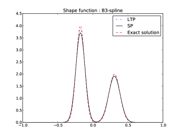
Shape functions for the particle method are here B3-splines given by (2.13). We first examine the validation of our code by comparison of the numerical solution and the exact solution of (1.1) with $W(x)=x^{2}$. Due to the conservation of the center of mass,

$$\forall t\geq 0,\qquad\int_{\mathbb{R}}x\rho(t,x)dx=\int_{\mathbb{R}}x\rho^{0}(x)dx:=\lambda\,,$$

the solution is explicitly given by

(6.4) $$\rho(t,x)=\rho^{0}\left((x-\lambda)e^{2t}+\lambda\right)e^{2t}\,,$$

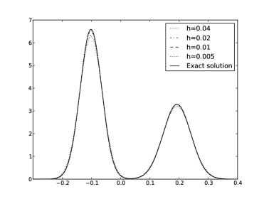
using the method of characteristics. Figure 2 (left) shows the exact solution of (1.1) with initial data (6.1) and the numerical solution computed with the LTP method, together with the $L^{1}$ and $L^{\infty}$ errors with respect to $h$.

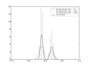
Let us now compare the results with classical particle methods. One of the drawbacks of classical particle methods in which the density is reconstructed with shape function of same size

$$\rho_{\varepsilon}^{n}(x)=\sum_{k\in\mathbb{Z}}\omega_{k}\frac{1}{\varepsilon}\varphi\left(\frac{x-x_{k}^{n}}{\varepsilon}\right)\,,$$

is the need to choose adequate values of $\varepsilon$. Indeed, if $\varepsilon$ is too small compared to the distance between two particles, the reconstructed density will vanish between particles and is thus irrelevant; and if $\varepsilon$ is too large the reconstructed density will be too spread out and the results lack accuracy, as it is demonstrated in Figure 2 (right).
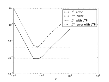
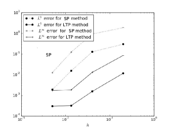
Refer to caption
Refer to caption
Figure 3. Left Figure: Log-Log Plot of the $L^{1}$ and $L^{\infty}$ errors of the SP method using various values for the particle radius $\varepsilon$, versus those of the LTP method (both using $h=0.01$ and $\Delta t=0.01$). Right Figure: Log-Log Plot of the $L^{1}$ and $L^{\infty}$ errors for the SP and LTP methods with $\Delta t=0.0001$ and different values of $h=\varepsilon$. In both cases, $W(x)=x^{2}$ and $\rho^{0}$ is given by (6.1) with errors computed at $t=0.5$.

Figure 3 presents the $L^{1}$ and $L^{\infty}$ errors between a standard Smooth Particle (SP) method (with different values of $\varepsilon$) and our LTP method for the potential $W(x)=x^{2}$ for which solutions are explicit by the method of characteristics, see (6.4). On the left picture, we observe that the optimal $\varepsilon$, at this instant $t$, for a classical particle method is well captured with the LTP method.

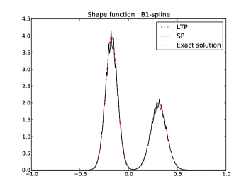
One could object that the gain is not significantly better with the LTP method. However, since particles aggregate, the average distance between two particles decreases exponentially in time, and consequently the optimal size $\varepsilon$ for reconstruction in classical particle method is not the same during the whole simulation. Therefore, an evolution in time of $\varepsilon$ is much better adapted. Notice that the case of potential $W(x)=x^{2}$ is not particularly the best example to show the higher accuracy of the LTP method with respect to the classical particle method since all particles have the same size at time $t$ because $j_{\mathrm{ex}}^{0,t}(x)=e^{-2t}$, see (6.4). Moreover, the gain of accuracy with the LTP method is even clearer while using B1-spline as shape functions instead of B3-spline, as it is demonstrated on Figure 4.

Refer to caption
Refer to caption
Figure 4. Comparisons between exact solution (at $t=0.5$) and approximated solutions $\rho_{h}^{n}$ with LTP method and SP method, with $W(x)=x^{2}/2$, $\rho^{0}$ given by (6.1), $h=1/25$ and $\Delta t=10^{-3}$. On the left Figure, the shape function $\varphi$ is a hat function, whereas on the right Figure, $\varphi$ is a B3-spline.

6.2. Numerical Simulations

We now take advantage of the method to explore the behavior for other attractive potentials of type $W(x)=\tfrac{|x|^{a}}{a}$, $a>1$. Notice that for $a\geq 2$ the potential is smooth while for $1<a<2$ is singular once $W$ is cut-off at infinity or if the initial data is compactly supported since the effective values of the potential lie on a bounded set and $W$ can be cut-off at infinity without changing the solution. Figure 5 presents the numerical results obtained by the LTP method in the case of $a=1.5$ and $a=2.5$. We represent the approximation of the density $\rho_{h}^{n}$, and also the reconstructed velocity $u_{h}^{n}$ and the reconstructed size of particles $h^{n}$ by piecewise linear interpolation such that

$$u_{h}^{n}(x_{k}^{n})=-\nabla W*\rho_{h}^{n}(x_{k}^{n}),\qquad\mbox{and}\qquad h^{n}(x_{k}^{n})=h\prod_{m=0}^{n-1}j_{k}^{m}.$$
$a=1.5$ $a=2.5$
Potential $W$ Refer to caption Refer to caption
Density $\rho_{h}^{n}$ Refer to caption Refer to caption
Velocity $\nabla W\ast\rho_{h}^{n}$ Refer to caption Refer to caption
Size of particles $h_{k}^{n}$ Refer to caption Refer to caption
Figure 5. Approximated density and reconstructed velocity and size of particles computed by the LTP method with $h=0.01$ for $W(x)=\tfrac{|x|^{a}}{a}$, with $a=1.5$ or $a=2.5$ and $\rho^{0}$ given by (6.2) with the number of time-steps $N=200$.

Potentials and their derivatives are also represented. In both cases, we observe that the density converges to a Dirac mass. Figure 5 also shows that for $a=2.5$, $W^{\prime\prime}\in L_{loc}^{\infty}$, no finite-time blow-up in $L^{\infty}$ appears, opposite to the case $a=1.5$ in agreement with the results proved in [7]. Notice also the different qualitative behavior in their trend to blow-up as studied in [40].

$b=1.1$ $b=1.5$ $b=2.5$
Potential $W$ Refer to caption Refer to caption Refer to caption
Density $\rho_{h}^{n}$ Refer to caption Refer to caption Refer to caption
Velocity $\nabla W\ast\rho_{h}^{n}$ Refer to caption Refer to caption Refer to caption
Size of particles $h_{k}^{n}$ Refer to caption Refer to caption Refer to caption
Figure 6. Approximated density and reconstructed velocity and size of particles computed by the LTP method with $h=0.01$ for $W(x)=\frac{|x|^{a}}{a}-\frac{|x|^{b}}{b}$, with $a=3$ and $b=1.5$ or $b=2.5$ and $\rho^{0}$ given by (6.2) with the number of time-steps $N=200$.

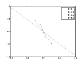
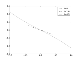
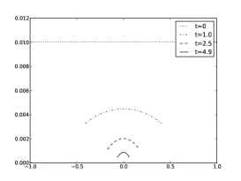
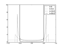
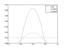
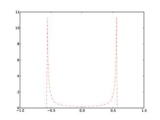
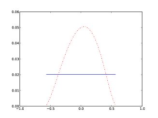
Now, we further analyse the blow-up behavior by looking at the case of attractive-repulsive potentials $W(x)=\tfrac{|x|^{a}}{a}-\tfrac{|x|^{b}}{b}$, $1<b<a$. Notice again that for $b\geq 2$ the potential is smooth while for $1<b<2$ is singular once $W$ is cut-off at infinity or if the initial data is compactly supported as discussed above. Figure 6 presents the approximated density $\rho_{h}^{n}$, reconstructed velocity $u_{h}^{n}$ and size of particles $h^{n}$ obtained by the LTP method in the case of the attractive-repulsive potentials with $(a,b)=(3,1.5)$ and $(a,b)=(3,2.5)$. In this case $\rho^{0}$ is given by (6.2).

We observe that the long time asymptotics for $b=2.5$ are characterized by the concentration of mass equally onto Dirac deltas at two points in infinite time, while for $b=1.5$ we obtain a convergence in time towards a steady $L^{1}$ density profile seemingly diverging at the boundary of the support. This last behavior has been reported in several simulations and related problems [6]. However, it has not been rigorously proven yet. Let us point out that the set of stationary states when the interaction potential is analytic in 1D consists of a finite number of Dirac deltas as proven in [35, 36]. This result also holds for $W(x)=\tfrac{|x|^{a}}{a}-\tfrac{|x|^{b}}{b}$, $2<b<a$, as it will be reported in [23].

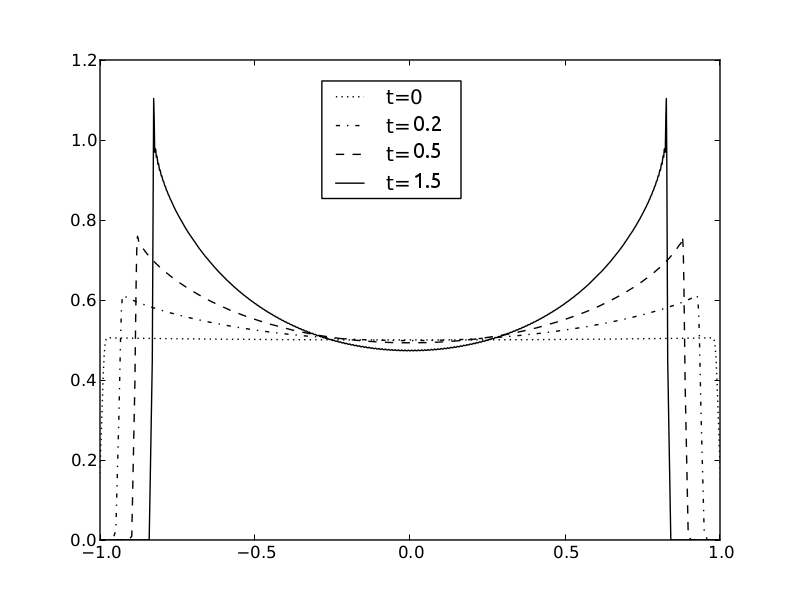
Figure 7 also represents the time evolution of the approximated density for $(a,b)=(3,2.5)$, with $\rho^{0}$ given by (6.3). Solutions in the range $2<b<a$ for initial data in $L^{1}\cap L^{\infty}$ exist globally in time, see [37]. The numerical evidence shows that all solutions converge towards stationary states consisting of finite number of Dirac Deltas as $t\to\infty$ in this range.

Refer to caption
Figure 7. Time evolution of the density for $W(x)=\frac{|x|^{a}}{a}-\frac{|x|^{b}}{b}$, with $a=3$, $b=2.5$ and $\rho^{0}$ given by (6.3) with $N=100$.

Finally, we show in Figure 8 the results of the stationary state of the SP method versus the LTP method for the potential $(a,b)=(4,2.5)$ with $N=100$. We observe how the good local adaption of the size of the particles makes our approximation much better with no oscillations with respect to the SP method showing the good performance of the LTP method in this case and its good properties at work. As mentioned in the introduction, vortex-blob type methods have been shown to converge for the aggregation equation (1.1). They obtained convergence estimates in suitable $L^{p}$ norms for the velocity fields and the associated characteristics fields while the error for the densities was controlled in suitable $W^{-1,p}$-norms in [8, Th. 3.8]. The error estimates for vortex-blob and SP methods depend as usual on the regularization of particles and the fixed particle size related in a suitable way to get convergence. We have proven that the LTP method has in contrast direct error estimates for the densities in $L^{p}$ depending on the initial mesh size showing that the local adaptation of the shape has this benefit on the error estimates too.

Refer to caption
Refer to caption
Refer to caption
Figure 8. Densities at steady state for $W(x)=\frac{|x|^{a}}{a}-\frac{|x|^{b}}{b}$, with $a=4$, $b=2.5$ and $\rho^{0}$ given by (6.2). Left Top: SP method (solid line), right top: LTP method (dotted line), bottom: size of particles (SP versus LTP) with $N=100$.

Appendix A A priori estimates on the regularity of solutions

In this part, we deduce a priori estimates on the regularity of equation (1.1) that combined with the global/local in time well posedness theory obtained in [32, 37, 10, 18], leads to the existence of solutions with the desired properties to apply the convergence results of previous sections.

As we remind the reader in the introduction and in several places along the text, there are two different well-posedness settings: for smooth and for singular potentials. In both cases under the assumptions on the initial data the velocity fields are continuous in time and Lipschitiz continuous in space. In the smooth potential case, this property holds globally in time leading to unique global in time measure solutions [32, 37]. In the singular potential case, this property holds locally in time only since there exist blowing-up of solutions for fully atractive potentials, see [7, 10, 18]. In both cases, the flow map associated to the velocity field is well-defined and solutions are obtained by pushing forward the initial data through the flow map.

In this Appendix, we present first a global-in-time propagation of regularity result in the smooth potential case adapted to our hypotheses on the convergence results. On the other hand, we show a local-in-time propagation of regularity result in the singular potential case.

Proposition 9.

Assume that the interaction potential $W$ satisfies $\nabla W\in\mathcal{W}^{1,\infty}(\mathbb{R}^{d})$. Let $T>0$ be given and $\rho$ be the unique weak solution to the system (1.1) with initial data $\rho^{0}\in\mathcal{W}_{+}^{1,1}(\mathbb{R}^{d})$ obtained in [32, 37], then

$$\sup_{0\leq t\leq T}\|\rho(t,\cdot)\|_{\mathcal{W}_{+}^{1,1}}\leq C,$$

where $C$ is a positive constant depending only on $T$, $L$, and $\|\rho^{0}\|_{\mathcal{W}_{+}^{1,1}}$. Furthermore, if we assume that the initial data $\rho^{0}\in(L^{\infty}\cap\mathcal{W}_{+}^{1,1})(\mathbb{R}^{d})$, then

$$\sup_{0\leq t\leq T}\|\rho(t,\cdot)\|_{L^{\infty}\cap\mathcal{W}^{1,1}_{+}}\leq C,$$

where $C$ is a positive constant depending only on $T$, $L$, and $\|\rho^{0}\|_{L^{\infty}\cap\mathcal{W}_{+}^{1,1}}$.

Proof.

It follows from the conservation of mass and our assumption on the initial data $\rho^{0}$ that

$$\int_{\mathbb{R}^{d}}\rho(t,x)\,dx=\int_{\mathbb{R}^{d}}\rho^{0}(x)\,dx=1.$$

For the estimate of $\|\rho\|_{L^{\infty}(0,T;\dot{\mathcal{W}}^{1,1})}$, we take $\nabla$ to (1.1) to get

(A.1) $\displaystyle\begin{aligned} \partial_{t}\nabla\rho(t,x)&+D^{2}\rho(t,x)u(t,x)+\nabla u(t,x)\nabla\rho(t,x)\cr&\quad+\nabla(\nabla\cdot u(t,x))\rho(t,x)+\nabla\cdot u(t,x)\nabla\rho(t,x)=0.\end{aligned}$

We next multiply (A.1) by $\nabla\rho(t,x)/|\nabla\rho(t,x)|$ to obtain

(A.2) $\displaystyle\begin{aligned} \partial_{t}|\nabla\rho|&+u\cdot\nabla|\nabla\rho(t,x)|+\nabla\cdot u|\nabla\rho(t,x)|=\cr&\quad-\nabla u\nabla\rho\cdot\frac{\nabla\rho}{|\nabla\rho|}-\nabla(\nabla\cdot u)\rho\cdot\frac{\nabla\rho}{|\nabla\rho|},\end{aligned}$

due to the symmetry of $D^{2}\rho$. By integrating (A.2) over $\mathbb{R}^{d}$ and using integration by parts, we deduce

(A.3) $\displaystyle\begin{aligned} \frac{d}{dt}\int_{\mathbb{R}^{d}}|\nabla\rho|\,dx=&-\int_{\mathbb{R}^{d}}\nabla u\nabla\rho\cdot\frac{\nabla\rho}{|\nabla\rho|}\,dx\cr&-\int_{\mathbb{R}^{d}}\nabla(\nabla\cdot u)\rho\cdot\frac{\nabla\rho}{|\nabla\rho|}\,dx\leq 2L|\nabla\rho|\,dx,\end{aligned}$

where we used $\|\nabla u(t,x)\|_{L^{\infty}}\leq\|\nabla W\|_{\mathcal{W}^{1,\infty}}=L$ and

$$\|\nabla(\nabla\cdot u)\|_{L^{\infty}}\leq L\int_{\mathbb{R}^{d}}|\nabla\rho|\,dx.$$

Thus we have

$$\sup_{0\leq t\leq T}\|\nabla\rho(t,\cdot)\|_{L^{1}}\leq\|\nabla\rho^{0}\|_{L^{1}}\exp\left(2LT\right).$$

Finally, we estimate $\|\rho\|_{L^{\infty}}$. For this, we recall that the flow map $F^{0,t}(x)$ satisfies

$$\frac{dF^{0,t}(x)}{dt}=u(t,F^{0,t}(x))\quad\mbox{with}\quad F^{0,0}(x)=x.$$

Using that $\rho(t)=F^{0,t}\#\rho^{0}$, we can write

$$\frac{\partial}{\partial t}\rho(t,F^{0,t}(x))=-\nabla\cdot u(t,F^{0,t}(x))\rho(t,F^{0,t}(x)),$$

and this yields

$$\rho(t,F^{0,t}(x))=\rho^{0}(x)\exp\left(-\int_{0}^{t}\nabla\cdot u(s,F^{0,s}(x))\,ds\right).$$

Since $u\in\mathcal{W}^{1,\infty}(\mathbb{R}^{d})$, we obtain

(A.4) $$\sup_{0\leq t\leq T}\|\rho(t,\cdot)\|_{L^{\infty}}\leq\|\rho^{0}\|_{L^{\infty}}\exp\left(LT\right).$$

This completes the proof. ∎

Remark 5.

If we further assume that $\rho^{0}\in\mathcal{W}_{+}^{1,\infty}(\mathbb{R}^{d})$, we have

$$\sup_{0\leq t\leq T}\|\rho(t,\cdot)\|_{\mathcal{W}^{1,\infty}}\leq C,$$

where $C$ is a positive constant depending only on $T$, $L$, and $\|\rho^{0}\|_{\mathcal{W}^{1,\infty}_{+}}$. Indeed, we can similarly find from (A.1) that for $i=1,\cdots,d$

$\displaystyle\frac{\partial}{\partial t}\partial_{i}\rho(t,F^{0,t}(x))$ $\displaystyle=-\partial_{i}u(t,F^{0,t}(x))\nabla\rho(t,F^{0,t}(x))-\nabla\cdot u(t,F^{0,t}(x))\partial_{i}\rho(t,F^{0,t}(x))$
$\displaystyle\quad-\rho(t,F^{0,t}(x))\nabla\cdot\partial_{i}u(t,F^{0,t}(x)).$

This implies

$\displaystyle\|\nabla\rho(t,\cdot)\|_{L^{\infty}}$ $\displaystyle\leq\|\nabla\rho_{0}\|_{L^{\infty}}\exp\left(C\int_{0}^{t}\|\nabla u(s,\cdot)\|_{L^{\infty}}\,ds\right)$
$\displaystyle\quad+\exp\left(C\int_{0}^{t}\|\nabla u(s,\cdot)\|_{L^{\infty}}\,ds\right)\int_{0}^{t}\|\rho(s,\cdot)\|_{L^{\infty}}\|D^{2}u(s,\cdot)\|_{L^{\infty}}\,ds,$
$\displaystyle\leq C\|\nabla\rho_{0}\|_{L^{\infty}}+C\int_{0}^{t}\|D^{2}u(s,\cdot)\|_{L^{\infty}}\,ds$

where we used $u\in\mathcal{W}^{1,\infty}(\mathbb{R}^{d})$ and the estimate (A.4). On the other hand, $\|D^{2}u(s,\cdot)\|_{L^{\infty}}$ can be estimated by

$$\|D^{2}u(s,\cdot)\|_{L^{\infty}}\leq\|\nabla W\|_{\mathcal{W}^{1,\infty}}\|\nabla\rho(s,\cdot)\|_{L^{\infty}}.$$

Hence, we have

$$\|\nabla\rho(t,\cdot)\|_{L^{\infty}}\leq C\|\nabla\rho_{0}\|_{L^{\infty}}+C\int_{0}^{t}\|\nabla\rho(s,\cdot)\|_{L^{\infty}}\,ds,$$

and by applying Gronwall’s inequality to conclude the desired result. Similar arguments were used in [2] to construct classical solutions.

We next provide the a priori estimate of solutions to the system (1.1) in $\mathcal{W}^{1,1}_{+}(\mathbb{R}^{d})\cap\mathcal{W}^{1,p}(\mathbb{R}^{d})$. For notational simplicity, we set

$$\widetilde{\mathcal{W}}^{k,p}_{+}(\mathbb{R}^{d}):=\mathcal{W}^{k,1}_{+}(\mathbb{R}^{d})\cap\mathcal{W}^{k,p}(\mathbb{R}^{d})\quad\mbox{for}\quad k\geq 0.$$
Proposition 10.

Assume that the interaction potential $W$ satisfies (5.1) for some $1\leq q\leq\frac{d}{\alpha+1}$. Let $\rho$ be the unique local-in-time solution to (1.1) constructed in [18] with initial data $\rho^{0}$ satisfying $\rho^{0}\in(L^{\infty}\cap\widetilde{\mathcal{W}}_{+}^{1,p})(\mathbb{R}^{d})$ where $p$ is the Sobolev conjugate of $q$. Then there exists a $T^{*}>0$ such that

$$\sup_{0\leq t\leq T^{*}}\|\rho(t,\cdot)\|_{\widetilde{\mathcal{W}}^{1,p}_{+}}\leq C,$$

where $C$ is a positive constant depending only on $T^{*}$, $\alpha$, $p$, and $\|\rho^{0}\|_{\widetilde{\mathcal{W}}^{1,p}_{+}}$.

Proof.

The local-in-time well-posedness theory in [18] that

(A.5) $$\frac{d}{dt}\|\rho\|_{\widetilde{\mathcal{W}}^{0,p}_{+}}\leq C\|\rho\|_{\widetilde{\mathcal{W}}^{0,p}_{+}}^{2}\,.$$

It also follows from (A.1)-(A.3) that

$$\frac{d}{dt}\|\nabla\rho\|_{L^{1}}\lesssim\|\rho\|_{\widetilde{\mathcal{W}}^{0,p}_{+}}\|\nabla\rho\|_{L^{1}}+\|\nabla\rho\|_{\widetilde{\mathcal{W}}^{0,p}_{+}}\leq\|\rho\|_{\widetilde{\mathcal{W}}^{1,p}_{+}}^{2},$$

where we used $\|D^{k}u(t,x)\|_{L^{\infty}}\leq C\|D^{k-1}\rho\|_{\widetilde{\mathcal{W}}^{0,p}_{+}}$ for $k\geq 1$ and $\|\rho\|_{\widetilde{\mathcal{W}}^{0,p}_{+}}\geq 1$. For the estimate of $\|\nabla\rho\|_{L^{p}}$, we obtain

$\displaystyle\frac{d}{dt}\int_{\mathbb{R}^{d}}|\nabla\rho|^{p}dx$ $\displaystyle=-p\int_{\mathbb{R}^{d}}|\nabla\rho|^{p-2}\nabla\rho\cdot\left(D^{2}\rho u+\nabla u\nabla\rho+\nabla(\nabla\cdot u)\rho+\nabla\cdot u\nabla\rho\right)dx$
$\displaystyle=(a)+(b)+(c)+(d),$

where $(a),(b),(c)$, and $(d)$ are estimated as follows.

$\displaystyle(a)$ $\displaystyle=-\int_{\mathbb{R}^{d}}u\cdot\nabla|\nabla\rho|^{p}dx=\int_{\mathbb{R}}\nabla\cdot u|\nabla\rho|^{p}dx\lesssim\|\rho\|_{\widetilde{\mathcal{W}}^{0,p}_{+}}\|\nabla\rho\|_{L^{p}}^{p},$
$\displaystyle(b)$ $\displaystyle\leq p\int_{\mathbb{R}^{d}}|\nabla u||\nabla\rho|^{p}dx\lesssim\|\rho\|_{\widetilde{\mathcal{W}}^{0,p}_{+}}\|\nabla\rho\|_{L^{p}}^{p},$
$\displaystyle(c)$ $\displaystyle\leq p\|\nabla^{2}u\|_{L^{\infty}}\|\rho\|_{L^{p}}\|\nabla\rho\|_{L^{p}}^{p-1}\lesssim\|\nabla\rho\|_{\widetilde{\mathcal{W}}^{0,p}_{+}}\|\rho\|_{L^{p}}\|\nabla\rho\|_{L^{p}}^{p-1},$
$\displaystyle(d)$ $\displaystyle\leq p\int_{\mathbb{R}^{d}}|\nabla\cdot u||\nabla\rho|^{p}dx\lesssim\|\rho\|_{\widetilde{\mathcal{W}}^{0,p}_{+}}\|\nabla\rho\|_{L^{p}}^{p}.$

Thus, we get

(A.6) $$\frac{d}{dt}\|\nabla\rho\|_{L^{p}}\leq C\|\rho\|_{\widetilde{\mathcal{W}}^{1,p}_{+}}^{2}.$$

Now, we combine (A.5) and (A.6) to deduce

$$\frac{d}{dt}\|\rho\|_{\widetilde{\mathcal{W}}^{1,p}_{+}}\leq C\|\rho\|_{\widetilde{\mathcal{W}}^{1,p}_{+}}^{2},$$

and this concludes that there exists a $T^{*}>0$ such that

$$\sup_{0\leq t\leq T}\|\rho(t,\cdot)\|_{\widetilde{\mathcal{W}}^{1,p}_{+}}\leq C,$$

where $C$ is a positive constant depending only on $T^{*}$, $\alpha$, $p$, and $\|\rho^{0}\|_{\widetilde{\mathcal{W}}^{1,p}_{+}}$.

Acknowledgments

JAC was partially supported by the project MTM2011-27739-C04-02 DGI (Spain) and from the Royal Society by a Wolfson Research Merit Award. JAC and YPC were supported by EPSRC grant with reference EP/K008404/1. This work was partially done when FC was visiting Imperial College funded by the EPSRC EP/I019111/1 (platform grant).

References

  • [1] L.A. Ambrosio, N. Gigli, and G. Savaré, Gradient flows in metric spaces and in the space of probability measures, Lectures in Mathematics, Birkhäuser, 2005.
  • [2] D. Balagué, J. A. Carrillo, T. Laurent, and G. Raoul. Nonlocal interactions by repulsive-attractive potentials: Radial ins/stability, Physica D, 260, (2013), 5–25.
  • [3] D. Balagué, J. A. Carrillo, T. Laurent, and G. Raoul, Dimensionality of local minimizers of the interaction energy, Arch. Rat. Mech. Anal., 209, (2013), 1055–1088.
  • [4] D. Balagué, J. A. Carrillo, and Y. Yao, Confinement for repulsive-attractive kernels, Disc. Cont. Dyn. Sys.-B, 19, (2014), 1227–1248.
  • [5] D. Benedetto, E. Caglioti, and M. Pulvirenti, A kinetic equation for granular media, RAIRO Modél. Math. Anal. Numér., 31, (1997), 615–641.
  • [6] A. J. Bernoff and C. M. Topaz, A primer of swarm equilibria, SIAM J. Appl. Dyn. Syst., 10, (2011), 212–250.
  • [7] A. Bertozzi, J. A. Carrillo, and T. Laurent, Blowup in multidimensional aggregation equations with mildly singular interaction kernels, Nonlinearity, 22, (2009), 683–710.
  • [8] A.L. Bertozzi and K. Craig, A blob method for the aggregation equation, to appear in Math. Comp.
  • [9] A. L. Bertozzi, T. Laurent, and F. Léger, Aggregation and spreading via the newtonian potential: the dynamics of patch solutions, Math. Models Methods Appl. Sci., 22(supp01):1140005, 2012.
  • [10] A.L. Bertozzi, T. Laurent, and J. Rosado, $L^{p}$ theory for the multidimensional aggregation equation, Comm. Pure Appl. Math., 43, (2010), 415–430.
  • [11] A. Blanchet and G. Carlier, From Nash to Cournot-Nash equilibria via the Monge-Kantorovich problem, Phil. Trans. R. Soc. A, 372: 20130398, 2014.
  • [12] M. Campos Pinto, Towards smooth particle methods without smoothing, J. Sci. Comput., (2014).
  • [13] M. Campos Pinto, F. Charles, Uniform convergence of a linearly transformed particle method for the Vlasov-Poisson system, preprint (2014).
  • [14] J.A. Cañizo, J.A. Carrillo, and J. Rosado, A well-posedness theory in measures for some kinetic models of collective motion, Math. Mod. Meth. Appl. Sci., 21, (2011), 515–539.
  • [15] J. A. Cañizo, J. A. Carrillo, F. S. Patacchini, Existence of Global Minimisers for the Interaction Energy, Arch. Rat. Mech. Anal., 217, (2015), 1197–1217.
  • [16] J. A. Carrillo, A. Chertock, and Y. Huang, A Finite-Volume Method for Nonlinear Nonlocal Equations with a Gradient Flow Structure, Comm. Comp. Phys., 17, (2015), 233–258.
  • [17] J. A. Carrillo, M. Chipot, and Y. Huang, On global minimizers of repulsive-attractive power-law interaction energies, Phil. Trans. R. Soc. A, 372:20130399, 2014.
  • [18] J. A. Carrillo, Y.-P. Choi, and M. Hauray, The derivation of swarming models: Mean-field limit and Wasserstein distances, Collective Dynamics from Bacteria to Crowds: An Excursion Through Modeling, Analysis and Simulation Series, CISM International Centre for Mechanical Sciences, 553, (2014), 1–46.
  • [19] J. A. Carrillo, M. G. Delgadino, and A. Mellet, Regularity of local minimizers of the interaction energy via obstacle problems, preprint, (2014).
  • [20] J. A. Carrillo, M. Di Francesco, A. Figalli, T. Laurent, and D. Slepčev, Global-in-time weak measure solutions and finite-time aggregation for nonlocal interaction equations, Duke Math. J., 156, (2011), 229–271.
  • [21] J. A. Carrillo, M. Di Francesco, A. Figalli, T. Laurent, and D. Slepčev, Confinement in nonlocal interaction equations, Nonlinear Anal., 75, (2012), 550–558.
  • [22] J. A. Carrillo, L. C. F. Ferreira, J. C. Precioso, A mass-transportation approach to a one dimensional fluid mechanics model with nonlocal velocity, Adv. Math., 231, (2012), 306–327.
  • [23] J. A. Carrillo, A. Figalli, F. S. Patacchini, work in progress.
  • [24] J. A. Carrillo, Y. Huang, S. Martin, Nonlinear stability of flock solutions in second-order swarming models, Nonlinear Analysis: Real World Applications, 17, (2014), 332–343.
  • [25] J. A. Carrillo, F. James, F. Lagoutière, N. Vauchelet, The Filippov characteristic flow for the aggregation equation with mildly singular potentials, preprint (2014).
  • [26] J. A. Carrillo, R. J. McCann, and C. Villani, Kinetic equilibration rates for granular media and related equations: entropy dissipation and mass transportation estimates, Rev. Mat. Iberoamericana, 19, (2003), 971–1018.
  • [27] J. A. Carrillo, R. J. McCann, and C. Villani, Contractions in the $2$-wasserstein length space and thermalization of granular media, Arch. Rat. Mech. Anal., 179, (2006), 217–263.
  • [28] P. G. Ciarlet, Basic error estimates for elliptic problems, vol. 2 of Handbook of Numerical Analysis. Elsevier, North-Holland, (1991), 17–351.
  • [29] A. Cohen, B. Perthame, Optimal Approximations of Transport Equations by Particle and Pseudoparticle Methods, SIAM J. on Math. Anal., 32, (2000), 616–636.
  • [30] G.-H. Cottet, P.-A. Raviart, Particle methods for the one-dimensional Vlasov-Poisson equations, SIAM J. Numer. Anal. 21, (1984), 52–76.
  • [31] P. Degond, J.-G. Liu, and C. Ringhofer, Evolution of the distribution of wealth in an economic environment driven by local Nash equilibria, J. Stat. Phys., 154, (2014), 751–780.
  • [32] R. Dobrushin, Vlasov equations, Funct. Anal. Appl., 13, (1979), 115–123.
  • [33] M. R. D’Orsogna, Y. Chuang, A. Bertozzi, and L. Chayes, Self-propelled particles with soft-core interactions: patterns, stability and collapse, Phys. Rev. Lett., 96(104302), 2006.
  • [34] J. P. K. Doye, D. J. Wales, and R. S. Berry, The effect of the range of the potential on the structures of clusters, J. Chem. Phys., 103, (1995), 4234–4249.
  • [35] K. Fellner and G. Raoul, Stable stationary states of non-local interaction equations, Math. Models Methods Appl. Sci., 20, (2010), 2267–2291.
  • [36] K. Fellner and G. Raoul, Stability of stationary states of non-local equations with singular interaction potentials, Math. Comput. Modelling, 53, (2011), 1436–1450.
  • [37] F. Golse, The Mean-Field Limit for the Dynamics of Large Particle Systems, Journées équations aux dérivées partielles, 9, (2003), 1–47.
  • [38] M. F. Hagan and D. Chandler, Dynamic pathways for viral capsid assembly, Biophysical Journal, 91, (2006), 42–54.
  • [39] M. Hauray, Wasserstein distances for vortices approximation of Euler-type equations, Math. Mod. Meth. Appl. Sci., 19, (2009), 1357–1384.
  • [40] Y. Huang, A. L. Bertozzi, Self-similar blowup solutions to an aggregation equation in $\mathbb{R}^{n}$, SIAM J. Appl. Math., 70, (2010), 2582–2603.
  • [41] F. James, N. Vauchelet, Chemotaxis: from kinetic equations to aggregate dynamics, NoDEA Nonlinear Differential Equations Appl., 20, (2013), 101–127.
  • [42] T. Kolokolnikov, J. A. Carrillo, A. Bertozzi, R. Fetecau, M. Lewis, Emergent behaviour in multi-particle systems with non-local interactions, Physica D: Nonlinear Phenomena, 260, (2013), 1–4.
  • [43] H. Li and G. Toscani, Long-time asymptotics of kinetic models of granular flows, Arch. Rat. Mech. Anal., 172, (2004), 407–428.
  • [44] A. J. Majda, A. L. Bertozzi, Vorticity and incompressible flow, Cambridge Texts in Applied Mathematics 27, Cambridge University Press, Cambridge 2002.
  • [45] A. Mogilner and L. Edelstein-Keshet, A non-local model for a swarm, J. Math. Bio., 38, (1999), 534–570.
  • [46] A. Mogilner, L. Edelstein-Keshet, L. Bent, and A. Spiros, Mutual interactions, potentials, and individual distance in a social aggregation, J. Math. Biol., 47, (2003), 353–389.
  • [47] G. Raoul, Non-local interaction equations: Stationary states and stability analysis, Differential Integral Equations, 25, (2012), 417–440.
  • [48] M. C. Rechtsman, F. H. Stillinger, and S. Torquato, Optimized interactions for targeted self-assembly: application to a honeycomb lattice, Phys. Rev. Lett., 95, (2005).
  • [49] C. Villani, Topics in optimal transportation, vol. 58 of Graduate Studies in Mathematics. Amer. Math. Soc., Providence, RI, 2003.
  • [50] J. von Brecht and D. Uminsky, On soccer balls and linearized inverse statistical mechanics, J. Nonlinear Sci., 22, (2012), 935–959.
  • [51] J. von Brecht, D. Uminsky, T. Kolokolnikov, and A. Bertozzi, Predicting pattern formation in particle interactions, Math. Mod. Meth. Appl. Sci., 22:1140002, 2012.
  • [52] D. J. Wales, Energy landscapes of clusters bound by short-ranged potentials, Chem. Eur. J. Chem. Phys., 11, (2010), 2491–2494.