Krylov approximation of ODEs with
polynomial parameterization

Abstract

We propose a new numerical method to solve linear ordinary differential equations of the type $\frac{\partial u}{\partial t}(t,\varepsilon)=A(\varepsilon)\,u(t,\varepsilon)$, where $A:\mathbb{C}\rightarrow\mathbb{C}^{n\times n}$ is a matrix polynomial with large and sparse matrix coefficients. The algorithm computes an explicit parameterization of approximations of $u(t,\varepsilon)$ such that approximations for many different values of $\varepsilon$ and $t$ can be obtained with a very small additional computational effort. The derivation of the algorithm is based on a reformulation of the parameterization as a linear parameter-free ordinary differential equation and on approximating the product of the matrix exponential and a vector with a Krylov method. The Krylov approximation is generated with Arnoldi’s method and the structure of the coefficient matrix turns out to have an independence on the truncation parameter so that it can also be interpreted as Arnoldi’s method applied to an infinite dimensional matrix. We prove the superlinear convergence of the algorithm and provide a posteriori error estimates to be used as termination criteria. The behavior of the algorithm is illustrated with examples stemming from spatial discretizations of partial differential equations.

1 Introduction

Let $A_{0}$, $A_{1}$, …, $A_{N}\in\mathbb{C}^{n\times n}$ be given matrices and consider the parameterized linear time-independent ordinary differential equation

(1.1) $$\frac{\partial u}{\partial t}(t,\varepsilon)=A(\varepsilon)\,u(t,\varepsilon),\quad u(0,\varepsilon)=u_{0},$$

where $A$ is the matrix polynomial $A(\varepsilon):=A_{0}+\varepsilon A_{1}+\cdots+\varepsilon^{N}A_{N}$. Although most of our results are general, the usefulness of the approach is more explicit in a setting where $N$ is not very large and the matrices $A_{0}$, …, $A_{N}$ are large and sparse, e.g., stemming from a spatial finite-element semi-discretization of a parameterized partial-differential equation of evolutionary type.

We present a new iterative algorithm for the parameterized ODE (1.1), which gives an explicit parameterization of the solution. This parameterization is explicit in the sense that after executing the algorithm we can find a solution to the ODE (1.1) for many different values of $\varepsilon$ and $t>0$ without essential additional computational effort. Such explicit parameterizations of solutions are useful in various settings, e.g., in parametric model order reduction and in the field of uncertainty quantification (with a single model parameter); see the discussion of model reduction below and the references in [3].

The parameterization of the solution is represented as follows. Let the coefficients of the Taylor expansion of the solution with respect to the parameter $\varepsilon$ be denoted by $c_{0}(t)$, $c_{1}(t)$, …, i.e.,

(1.2) $$u(t,\varepsilon)=\exp(tA(\varepsilon))\,u_{0}=\sum\limits_{\ell=0}^{\infty}\varepsilon^{\ell}c_{\ell}(t).$$

As $\,\exp\left(tA(\varepsilon)\right)\,$ is an entire function of a matrix polynomial, the expansion (1.2) exists for all $\varepsilon\in\mathbb{C}$.

Consider the approximation stemming from the truncation of the Taylor series (1.2) and a corresponding approximation of the Taylor coefficients

$$u_{k}(t,\varepsilon) :=\sum\limits_{\ell=0}^{k-1}\varepsilon^{\ell}c_{\ell}(t)$$

(1.3) $$\approx\sum\limits_{\ell=0}^{k-1}\varepsilon^{\ell}\widetilde{c}_{\ell}(t)=:\widetilde{u}_{k}(t,\varepsilon).$$

Our approach gives an explicit parameterization with respect $t$ of the approximate coefficients $\widetilde{c}_{0}(t)$,…,$\widetilde{c}_{k-1}(t)$ which, via (1.3), gives an approximate solution with an explicit parameterization with respect to $\varepsilon$ and $t$.

The derivation of our approach is based on an explicit characterization of the time-dependent coefficients $c_{0}(t)$,…,$c_{m-1}(t)$. We prove in Section 2 that they are solutions to the linear ordinary differential equation of size $nm$,

(1.4) $$\frac{\hskip 1.0pt{\rm d}\hskip 0.5pt}{\hskip 1.0pt{\rm d}\hskip 0.5ptt}\begin{bmatrix}c_{0}(t)\\ \vdots\\ c_{m-1}(t)\end{bmatrix}=L_{m}\begin{bmatrix}c_{0}(t)\\ \vdots\\ c_{m-1}(t)\end{bmatrix},\qquad\begin{bmatrix}c_{0}(0)\\ \vdots\\ c_{m-1}(0)\end{bmatrix}=\begin{bmatrix}u_{0}\\ 0\\ \vdots\\ 0\end{bmatrix}.$$

The matrix $L_{m}$ in (1.4) is a finite-band block Toeplitz matrix and also a lower block triangular matrix.

Since (1.4) is a standard linear ODE, we can in principle apply any numerical method to compute the solution which results in approximate coefficients $\widetilde{c}_{0}(t)$,…,$\widetilde{c}_{m-1}(t)$. Exponential integrators combined with Krylov approximation of matrix functions have recently turned out to be an efficient class of methods for large-scale (semi)linear ODEs arising from PDEs [11, 12]. See also [13] for a recent summary of exponential integrators. Krylov approximations of matrix functions have a feature which is suitable in our setting: after one run they give parameterized approximations with respect to the time-parameter.

Our derivation is based on approximating the solution of (1.4), i.e., a product of the matrix exponential and a vector, using a Krylov method. This is done by exploiting the structure of the coefficient matrix $L_{m}$. We show that when we apply Arnoldi’s method to construct a Krylov subspace corresponding to (1.4), the block Toeplitz and lower block triangular property of $L_{m}$ result in a particular structure in the basis matrix given by Arnoldi’s method.

The structure of $L_{m}$ is such that, in a certain sense, the algorithm can be equivalently extended to infinity. For example when $N=1$, the basis matrix is extended with one block row as well as a a block column in every iteration. This is analogous to the infinite Arnoldi method which has been developed for nonlinear eigenvalue problems [15] and linear inhomogeneous ODEs [16]. This feature implies that the algorithm does not require an a priori choice of the truncation parameter $m$.

We prove convergence of the algorithm (in Section 3) and also provide a termination criteria by giving a posteriori error estimates in Section 4.

The results can be interpreted and related to other approaches from a number of different perspectives. From one viewpoint, our result is related to recent work on computations and theory for Fréchet derivatives of matrix functions, e.g., [10, 19, 18]. As an illustration of a relation, consider the special case $N=1$. The first-order expansion of the matrix exponential in (1.2) and [9, Chapter 3.1] gives

$$u(t,\varepsilon) =\exp(t(A_{0}+\varepsilon A_{1}))\,u_{0}$$

$$=\exp(tA_{0})\,u_{0}+L_{\exp}(tA_{0},\varepsilon tA_{1})\,u_{0}+o(|\varepsilon|\,|t|\,\|A_{1}\|),$$

where $L_{\exp}$ is the Fréchet derivative of the matrix exponential. Since the Fréchet derivative is linear in the second parameter, the first coefficient is explicitly given by $c_{1}(t)=L_{\exp}(tA_{0},tA_{1})\,u_{0}$. The higher order terms $c_{2},c_{3},\ldots$ have corresponding relationships with the higher order Fréchet derivatives. An analysis of higher order Fréchet derivatives is given in [20]. In contrast to the current Fréchet derivative approaches, our approach is an iterative Krylov method with a focus on large and sparse matrices and a specific starting vector, which unfortunately does not appear to be easily constructed within the Fréchet derivative framework.

The general approach to compute parameterized solutions to parameterized problems is very common in the field of model order reduction (MOR). See the recent survey papers [3, 2]. In the terminology of MOR, our approach can be interpreted as a time-domain model order reduction technique for parameterized linear dynamical systems, without input or output. Parametric MOR is summarized in [3]; see also [17, 23]. Our approach is a Krylov method to compute a moment matching approximation in the model parameter $\varepsilon$. There are time-domain Krylov methods, e.g., those described in PhD thesis [6]. To our knowledge, none of these methods can be interpreted as exponential integrators.

We use the following notation in this paper. We let $\#S$ denote the number of elements in the set $S$, and $\operatorname{vec}(B)$ denote vectorization, i.e., $\operatorname{vec}(B)=[b_{1}^{T},\ldots,b_{k}^{T}]^{T}\in\mathbb{C}^{nk}$, where $B=[b_{1},\ldots,b_{k}]\in\mathbb{C}^{n\times k}$. By $I_{n}$ we indicate the identity matrix of dimension $n$. The set of eigenvalues of a matrix $A$ is denoted by $\Lambda(A)$ and the positive integers by $\mathbb{N}_{+}$. The logarithmic norm (or numerical abscissa) $\mu:\mathbb{C}^{n\times n}\rightarrow\mathbb{R}$ is defined by

(1.5) $$\mu(A):=\max\left\{\lambda\in\mathbb{R}\,:\,\lambda\in\Lambda\left(\frac{A+A^{*}}{2}\right)\right\}.$$

2 Derivation of the algorithm

2.1 Representation of the coefficients using the matrix exponential

To derive the algorithm, we first show that the time-dependent coefficients $c_{0}(t)$, …, $c_{m-1}(t)$ are solutions to a linear time-independent ODE of the form (1.4), i.e., they are explicitly given by the matrix exponential.

Theorem 1 (Explicit formula with matrix exponential).

The Taylor coefficients $c_{0}(t),\ldots,c_{m-1}(t)$ in (1.2) are explicitly given by

(2.1) $$\operatorname{vec}(c_{0}(t),\ldots,c_{m-1}(t))=\exp(tL_{m})\,\widetilde{u}_{0},$$

where

(2.2) $$L_{m}:=\begin{bmatrix}A_{0}&&&&&\\ A_{1}&\ddots&&&&\\ \vdots&\ddots&\ddots&&&\\ A_{\widehat{N}}&\ddots&\ddots&\ddots&&\\ &\ddots&\ddots&\ddots&\ddots&\\ &&A_{\widehat{N}}&\ldots&A_{1}&A_{0}\\ \end{bmatrix}\in\mathbb{C}^{mn\times mn}\quad\textrm{and}\quad\widetilde{u}_{0}=\begin{bmatrix}u_{0}\\ 0\\ \vdots\\ 0\end{bmatrix}\in\mathbb{C}^{mn},$$

and $\widehat{N}=\min(m-1,N)$.

Proof.

The proof is based on explicitly forming an associated ODE. The result can also be proven using a similar result [18, Theorem 4.1]. We give here an alternative shorter proof for the case of the matrix exponential, since some steps of the proof are needed in other parts of this paper. Differentiating (1.2) yields that for any $j\geq 0$,

(2.3) $$\frac{1}{j!}\frac{\partial^{j}}{\partial\varepsilon^{j}}u(t,\varepsilon)\bigg{|}_{\varepsilon=0}=c_{j}(t).$$

By evaluating (2.3) at $t=0$, and noting that $u(0,\varepsilon)=u_{0}$ is independent of $\varepsilon$, it follows that $c_{0}(0)=u_{0}$ and $c_{\ell}(0)=0$ for $\ell>0$. The initial value problem (1.1) and the expansion of its solution (1.2) imply that

(2.4) $$c_{j}^{\prime}(t) =\frac{1}{j!}\frac{\partial^{j}}{\partial\varepsilon^{j}}\frac{\partial}{\partial t}u(t,\varepsilon)\bigg{|}_{\varepsilon=0}=\frac{1}{j!}\frac{\partial^{j}}{\partial\varepsilon^{j}}\left(\sum\limits_{i=0}^{N}\varepsilon^{i}A_{i}\right)\,u(t,\varepsilon)\bigg{|}_{\varepsilon=0}$$

$$=\frac{1}{j!}\frac{\partial^{j}}{\partial\varepsilon^{j}}\sum\limits_{i=0}^{N}\varepsilon^{i}A_{i}\sum\limits_{\ell=0}^{\infty}\varepsilon^{\ell}c_{\ell}(t)\bigg{|}_{\varepsilon=0}$$

$$=\sum\limits_{i=0}^{N}\sum\limits_{\ell=0}^{\infty}\left(\frac{1}{j!}\frac{\partial^{j}}{\partial\varepsilon^{j}}\varepsilon^{i+\ell}\bigg{|}_{\varepsilon=0}\right)A_{i}c_{\ell}(t)$$

$$=\sum\limits_{i=0}^{\min(N,j)}A_{i}c_{j-i}(t).$$

From (2.3) and (2.4) it follows that the vector $\operatorname{vec}(c_{0}(t),\ldots,c_{m-1}(t))$ satisfies the linear ODE (1.4) with a solution given by (2.1). ∎

Input : $u_{0}\in\mathbb{C}^{n}$, $A_{0}$,…,$A_{N}\in\mathbb{C}^{n\times n}$

Output : Matrices $Q_{p}\in\mathbb{C}^{n(1+N(p-1))\times p}$ and $H_{p}\in\mathbb{C}^{p\times p}$ representing approximations of the coefficients $c_{0}$, …, $c_{p-1}$ via (2.7)

1 Let $\beta=\|u_{0}\|$, $Q_{1}=u_{0}/\beta$, $\underline{H}_{0}=[\ ]$

for $\ell=1,2,\ldots,p$ do

      2 Let $x=Q(:,\ell)\in\mathbb{C}^{n+(\ell-1)nN}$

      3 Compute $y:=\operatorname{vec}(y_{1},\dots,y_{1+(\ell-1)N})\in\mathbb{C}^{n+(\ell-1)nN}$ with (2.6)

      4 Let $\underline{Q}_{\ell}:=\begin{bmatrix}Q_{\ell}\\ 0\end{bmatrix}\in\mathbb{C}^{\ell\times(n+\ell nN)}$

      5 Compute $h=\underline{Q}_{\ell}^{*}w$

      6 Compute $y_{\perp}:=y-\underline{Q}_{\ell}h$

      7 Repeat Steps 1–1 if necessary

      8 Compute $\alpha=\|y_{\perp}\|$

      9 Let $\underline{H}_{\ell}=\begin{bmatrix}\underline{H}_{\ell-1}&h\\ 0&\alpha\\ \end{bmatrix}$

      10 Let $Q_{\ell+1}:=[\underline{Q}_{\ell},y_{\perp}/\alpha]\in\mathbb{C}^{(n+(\ell-1)nN)\times(\ell+1)}$

end for

11Let $H_{p}\in\mathbb{R}^{p\times p}$ be the leading submatrix of $\underline{H}_{p}\in\mathbb{R}^{(p+1)\times p}$

Algorithm 1 Infinite Arnoldi algorithm for polynomial uncertain ODEs

2.2 Algorithm

Theorem 1 can be used to compute the coefficients $c_{\ell}(t)$ if we can compute the matrix exponential of $L_{m}$ times the vector $\widetilde{u}_{0}$. We use a Krylov approximation which exploits the structure of the problem. See, e.g., [11, 12] for literature on Krylov approximations of matrix functions.

The Krylov approximation of $v(t)=\exp(tB)v_{0}$, consists of $p$ steps of the Arnoldi iteration for the matrix $B$ initiated with the vector $v_{0}$. This results in the Arnoldi relation

$$BQ_{p}=Q_{p+1}\underline{H}_{p},$$

where $\underline{H}_{p}\in\mathbb{C}^{(p+1)\times p}$ is a Hessenberg matrix and $Q_{p}$ is an orthogonal matrix spanning the Krylov subspace $\mathcal{K}_{p}(B,v_{0})=\operatorname{span}(v_{0},Bv_{0},\ldots,B^{p-1}v_{0})$. The Krylov approximation of $\exp(tB)v_{0}$ is given by

$$v(t)=\exp(tB)v_{0}\approx Q_{p}\exp(tH_{p})e_{1}\,\|v_{0}\|,$$

where $H_{p}\in\mathbb{C}^{p\times p}$ is the leading submatrix of $\underline{H}_{p}$, and $e_{1}$ is the first unit basis vector.

The only way $B$ appears in the Arnoldi algorithm is in the form of matrix vector products. Moreover, the Arnoldi algorithm is initiated with the vector $v_{0}$. Suppose we apply this Arnoldi approximation to (2.1). In the first step we need to compute the matrix vector product

(2.5) $$L_{m}\operatorname{vec}(u_{0},0,\dots,0)=\operatorname{vec}(A_{0}\,u_{0},\dots,A_{N}\,u_{0},0,\dots,0),$$

which is more generally given as follows.

Lemma 2 (Matrix vector product).

Suppose $x=\operatorname{vec}(x_{1},\dots,x_{j},0,\dots,0)=\operatorname{vec}(X)\in\mathbb{C}^{nm}$, where $x_{1},\ldots,x_{j}\in\mathbb{C}^{n}$ and $m>j+N$. Then,

$$L_{m}x=\operatorname{vec}(y_{1},\ldots,y_{j+N},0,\ldots,0),$$

where

(2.6) $$y_{\ell}=\sum_{i=\max(0,\ell-k)}^{\min(N,\ell-1)}A_{i}x_{\ell-i},\;\;\ell=1,\ldots,j+N.$$

Proof.

Suppose $S\in\mathbb{R}^{m\times m}$ is the shift matrix $S:=\sum_{\ell=1}^{m-1}e_{\ell+1}e_{\ell}^{T}$ which satisfies $(S^{i})^{T}=\sum_{\ell=1}^{m-i}e_{\ell}e_{\ell+i}^{T}$. We have

$$L_{m}x =\sum_{i=0}^{N}(S^{i}\otimes A_{i})\operatorname{vec}(X)=\sum_{i=0}^{N}\operatorname{vec}(A_{i}X(S^{i})^{T})$$

$$=\sum_{i=0}^{N}\sum_{\ell=1}^{m-i}\operatorname{vec}(A_{i}Xe_{\ell}e_{\ell+i}^{T}).$$

Note that $Xe_{\ell}=x_{\ell}$ if $\ell\leq j$ and $Xe_{\ell}=0$ if $\ell>j$. Hence, by using the assumption $m>j+N$, and reordering the terms in the sum we find the explicit formula $L_{m}x=\sum_{i=0}^{N}\sum_{\ell=1}^{j}\operatorname{vec}(A_{i}x_{\ell}e_{\ell+i}^{T})=\sum_{\ell=1}^{j+N}\sum_{i=\max(0,\ell-j)}^{\min(N,\ell-1)}\operatorname{vec}(A_{i}x_{\ell-i}e_{\ell}^{T})$. ∎

Since the Arnoldi method consists of applying matrix vector products and orthogonalizing the new vector against previous vectors, we see from (2.5) that the second vector in the Krylov subspace will consist of $N+1$ nonzero blocks. Repeated application of Lemma 2 results in a structure where the $j$th column in the basis matrix consists of $(j-1)N+1$ nonzero blocks, under the condition that $m$ is sufficiently large. It is natural to store only the nonzero blocks of the basis matrix. By only storing the nonzero blocks, the Arnoldi method for (2.1) reduces to Algorithm 1.

Note that our construction is equivalent to the Arnoldi method and the output of the algorithm is a basis matrix and a Hessenberg matrix which together form the approximation of the coefficients $c_{0},\ldots,c_{k-1}$

(2.7) $$\operatorname{vec}(c_{0}(t),\ldots,c_{k-1}(t))\approx\operatorname{vec}(\widetilde{c}_{0}(t),\ldots,\widetilde{c}_{k-1}(t)):=Q_{p}\exp(tH_{p})e_{1}\,\|u_{0}\|,$$

where by construction $k=N(p-1)$. The approximation of the solution is denoted as (1.3), i.e.,

$$\widetilde{u}_{k,p}(t):=\sum\limits_{\ell=0}^{k-1}\varepsilon^{\ell}\,\widetilde{c}_{\ell}(t),$$

where we added an index $p$ to stress the dependence on iteration. A feature of this construction is that the algorithm does not explicitly dependend on $m$, such that it in a sense can be extended to infinity, i.e., it is equivalent to Arnoldi’s method on an infinite dimensional operator. The result can be summarized as follows.

Theorem 3.

The following procedures generate identical results.

• $p$ iterations of Algorithm 1 started with $u_{0}$ and $A_{0}$, …, $A_{N}$;

• $p$ iterations of Arnoldi’s method applied to $L_{m}$ with starting vector $e_{1}\otimes u_{0}\in\mathbb{C}^{nm}$ for any $m\geq Np$;

• $p$ iterations of Arnoldi’s method applied to the infinite matrix $L_{\infty}$ with the infinite starting vector $e_{1}\otimes u_{0}\in\mathbb{C}^{\infty}$.

3 A priori convergence theory

To show the validity of our approach we now bound the total error after $p$ iterations, which is separated into two terms as

(3.1) $$\operatorname{err}_{p}(t,\varepsilon) :=\|u(t,\varepsilon)-\widetilde{u}_{N(p-1),p}(t,\varepsilon)\|$$

$$\,\,\leq\operatorname{err}_{{\rm K},N(p-1),p}(t,\varepsilon)+\operatorname{err}_{{\rm T},N(p-1)}(t,\varepsilon),$$

where

(3.2) $$\operatorname{err}_{{\rm K},k,p}(t,\varepsilon) :=\|\widetilde{u}_{k,p}(t,\varepsilon)-u_{k}(t,\varepsilon)\|$$

(3.3) $$\operatorname{err}_{{\rm T},k}(t,\varepsilon) :=\|u(t,\varepsilon)-u_{k}(t,\varepsilon)\|.$$

A bound of $\operatorname{err}_{{\rm K},k,p}$, which corresponds to the Krylov approximation of the expansion coefficients $c_{0},\ldots,c_{k-1}$, is given in Section 3.1 and a bound on $\operatorname{err}_{{\rm T},k}$, which corresponds to the truncation of the series, is given in Section 3.2. After combining the main results of Section 3.1 and Section 3.2, in particular formulas (3.8) and (3.9), we reach the conclusion that

(3.4) $$\operatorname{err}_{p}(t,\varepsilon)\leq\\ C_{1}(t,\varepsilon)\sum\limits_{\ell=0}^{N-1}\frac{C_{2}(t,\varepsilon)^{p+\ell-1}{\rm e}\hskip 1.0pt^{C_{2}(t,\varepsilon)}}{(p+\ell-2)!}\|u_{0}\|+2\sqrt{\frac{1-\left|\varepsilon\right|^{2N(p-1)}}{1-\left|\varepsilon\right|^{2}}}\frac{(t\alpha)^{p}{\rm e}\hskip 1.0pt^{t\gamma}}{p!}\|u_{0}\|,$$

where $\alpha$ and $\gamma$ are given in (3.6), and $C_{1}(t,\varepsilon)$ and $C_{2}(t,\varepsilon)$ are given in (3.10). Due to the factorial in the denominator of (3.4), for fixed $\varepsilon$ and $t>0$, the total error approaches zero superlinearly with respect to the iteration count $p$.

3.1 A bound on the Krylov error

We first study the error generated by the Arnoldi method to approximate the coefficients $c_{0}(t)$,…,$c_{k-1}(t)$. We define

(3.5) $$E_{k,p}(t)=[c_{0}(t),\ldots,c_{k-1}(t)]-[\widetilde{c}_{0}(t),\ldots,\widetilde{c}_{k-1}(t)].$$

where $\widetilde{c}_{0}$, …, $\widetilde{c}_{k}$ are the approximations given by the Arnoldi method, i.e., by the vector

$$\widehat{c}_{k}(t):=\begin{bmatrix}\widetilde{c}_{0}(t)\\ \vdots\\ \widetilde{c}_{k-1}(t)\end{bmatrix}=Q_{p}\exp(tH_{p})e_{1}\,\|u_{0}\|.$$

Using existing bounds for the Arnoldi approximation of the matrix exponential [8], we get a bound for the error of this approximation, as follows.

Lemma 4 (Krylov coefficient error bound).

Let $t>0$, $A_{0}$,…,$A_{N}\in\mathbb{C}^{n\times n}$, and $u_{0}\in\mathbb{C}^{n}$. Let $\widetilde{c}_{0}(t)$,…,$\widetilde{c}_{k-1}(t)$ be the result of Algorithm 1, and let $E_{k,p}(t)$ be defined by (3.5). Then, the total error in the coefficients $\|\operatorname{vec}(E_{k}(t))\|$ satisfies

$$\|\operatorname{vec}(E_{k,p}(t))\|=\|\exp(tL_{k})\widetilde{u}_{0}-\widehat{c}_{k}(t)\|\leq 2\,\frac{(t\alpha)^{p}}{p!}\,e^{t\max\{1,\beta\}}\,\|u_{0}\|$$

where

(3.6) $$\alpha=\sum_{\ell=0}^{N}\|A_{\ell}\|\quad\quad\textrm{and}\quad\quad\beta=\mu(A_{0})+\sum_{\ell=1}^{N}\|A_{\ell}\|,$$

and $\mu(B)$ denotes the logarithmic norm defined in (1.5)

Proof.

The result follows directly from [8, Thm. 2.1], and Lemma 8 and Corollary 10 in Appendix A. ∎

The coefficient error bound in Lemma 4, implies the following bound on the error $\operatorname{err}_{{\rm K},k,p}$, via the relation

(3.7) $$\operatorname{err}_{{\rm K},k,p}(t,\varepsilon)=\|E_{k,p}(t)[1,\varepsilon,\ldots,\varepsilon^{k-1}]^{T}\|.$$

Theorem 5 (Krylov error bound).

Let $\operatorname{err}_{{\rm K},k,p}$ be defined in (3.2) corresponding to applying $p$ steps of Algorithm 1 to $A_{0}$,…,$A_{N}\in\mathbb{C}^{n\times n}$ and $u_{0}\in\mathbb{C}^{n}$. Then,

(3.8) $$\operatorname{err}_{{\rm K},k,p}(t,\varepsilon)\leq 2\,\sqrt{\frac{1-\left|\varepsilon\right|^{2k}}{1-\left|\varepsilon\right|^{2}}}\ \frac{(t\alpha)^{p}{\rm e}\hskip 1.0pt^{t\max\{1,\beta\}}}{p!}\,\|u_{0}\|$$

where $\alpha$ and $\beta$ are given in (3.6).

Proof.

By (3.7) and the Cauchy–Schwarz inequality we have that

$$\operatorname{err}_{{\rm K},k,p}(t,\varepsilon) =\|\sum\limits_{\ell=0}^{k-1}\varepsilon^{\ell}({c}_{\ell}(t)-\widetilde{c}_{\ell}(t))\|$$

$$\leq\sqrt{\sum\limits_{\ell=0}^{k-1}\left|\varepsilon^{\ell}\right|^{2}}\ \sqrt{\sum\limits_{\ell=0}^{k-1}\|{c}_{\ell}(t)-\widetilde{c}_{\ell}(t)\|^{2}}$$

$$=\sqrt{\frac{1-\left|\varepsilon\right|^{2k}}{1-\left|\varepsilon\right|^{2}}}\ \|\operatorname{vec}(E_{k,p}(t))\|.$$

The claim follows now from Lemma 4. ∎

3.2 A bound on the truncation error

The previous subsection gives us an estimate for the error in the coefficient vectors $c_{\ell}(t)$. To characterize the total error of our approach, we now analyze the second term in the error splitting (3.1), i.e., the remainder

$$\operatorname{err}_{{\rm T},k}(t,\varepsilon):=\|u(t,\varepsilon)-\sum\limits_{\ell=0}^{k-1}\varepsilon^{\ell}c_{\ell}(t)\|.$$

Lemma 13 of Appendix gives a bound for the norms of $c_{\ell}(t)$ and can be used to derive the following theorem which bounds $\operatorname{err}_{{\rm T},k}(t,\varepsilon)$.

Theorem 6 (Remainder bound).

Let $c_{0}$,$c_{1}$,…be the coefficients of the $\varepsilon$-expansion (1.2) of $u(t,\varepsilon)$ when $N\geq 1$. Then, the error $\operatorname{err}_{{\rm T},k}(t,\varepsilon)$ is bounded as

(3.9) $$\operatorname{err}_{{\rm T},k}(t,\varepsilon)\leq C_{1}(t,\varepsilon)\sum\limits_{\ell=0}^{N-1}\frac{C_{2}(t,\varepsilon)^{\lfloor\frac{k}{N}\rfloor+\ell}}{(\lfloor\frac{k}{N}\rfloor+\ell-1)!},$$

where

(3.10) $$C_{1}(t,\varepsilon) =\left|\varepsilon\right|^{\mathrm{sign}(\left|\varepsilon\right|-1)}{\rm e}\hskip 1.0pt^{t(\mu(A_{0})+{\rm e}\hskip 1.0ptNa)+C_{2}(t,\varepsilon)-1}\|u_{0}\|,$$

$$C_{2}(t,\varepsilon) =\left|\varepsilon\right|^{N}{\rm e}\hskip 1.0ptNta.$$

Proof.

From Lemma 13 it follows that

$$\operatorname{err}_{{\rm T},k}(t,\varepsilon)=\|\sum_{\ell=k}^{\infty}\varepsilon^{\ell}c_{\ell}(t)\|\leq\sum_{\ell=k}^{\infty}\left|\varepsilon\right|^{\ell}\|c_{\ell}(t)\|\leq\widetilde{C}_{1}(t,\varepsilon)\sum\limits_{\ell=k}^{\infty}\left|\varepsilon\right|^{\ell}\frac{({\rm e}\hskip 1.0ptNta)^{\lceil\frac{\ell}{N}\rceil}}{(\lceil\frac{\ell}{N}\rceil-1)!},$$

where $\widetilde{C}_{1}(t,\varepsilon)={\rm e}\hskip 1.0pt^{t(\mu(A_{0})+{\rm e}\hskip 1.0ptNa)-1}\|u_{0}\|$.

Setting $\widetilde{k}=k-N\lfloor\frac{k}{N}\rfloor$ and using the bound $c^{\ell}=(c^{N})^{\frac{\ell}{N}}\leq(c^{N})^{\lceil\frac{\ell}{N}\rceil}c^{\mathrm{sign}(c-1)}$ for $c>0$, we get

$$\sum\limits_{\ell=k}^{\infty}\left|\varepsilon\right|^{\ell}\frac{({\rm e}\hskip 1.0ptNta)^{\lceil\frac{\ell}{N}\rceil}}{(\lceil\frac{\ell}{N}\rceil-1)!} \leq\left|\varepsilon\right|^{\mathrm{sign}(\left|\varepsilon\right|-1)}\sum\limits_{\ell=\widetilde{k}}^{\infty}\frac{(\left|\varepsilon\right|^{N}{\rm e}\hskip 1.0ptNta)^{\lceil\frac{\ell}{N}\rceil}}{(\lceil\frac{\ell}{N}\rceil-1)!}$$

$$=\left|\varepsilon\right|^{\mathrm{sign}(\left|\varepsilon\right|-1)}\sum\limits_{j=0}^{N-1}\sum\limits_{\ell=\lfloor\frac{k}{N}\rfloor+j}^{\infty}\frac{(\left|\varepsilon\right|^{N}{\rm e}\hskip 1.0ptNta)^{\ell}}{(\ell-1)!}.$$

Using the inequality [21, Lemma 4.2]

(3.11) $$\sum\limits_{\ell=k}^{\infty}\frac{x^{\ell}}{\ell!}\leq\frac{x^{k}{\rm e}\hskip 1.0pt^{x}}{k!}\quad\textrm{for}\quad x>0,$$

the claim follows. ∎

We also give a bound for the special case $N=1$ since it is in this case considerably lower than the one given in Theorem 6.

Theorem 7 (Remainder bound $N=1$).

Let $N=1$. Then the remainder $\operatorname{err}_{{\rm T},k}$ is bounded as

(3.12) $$\operatorname{err}_{{\rm T},k}(t,\varepsilon)\leq\frac{{\rm e}\hskip 1.0pt^{t(\mu(A_{0})+\left|\varepsilon\right|\|A_{1}\|)}(\left|\varepsilon\right|\|tA_{1}\|)^{k}}{k!}\|u_{0}\|.$$

Proof.

From Lemma 11 and (B.3) we see that $c_{\ell}(t)$ consists now of one integral term which can be bounded by Lemma 12 giving

$$\|c_{\ell}(t)\|\leq\frac{\|tA_{1}\|^{k}}{k!}\,{\rm e}\hskip 1.0pt^{t\mu(A_{0})}\,\|u_{0}\|.$$

Therefore

$$\operatorname{err}_{{\rm T},k}(t,\varepsilon)\leq\sum_{\ell=k}^{\infty}\left|\varepsilon\right|^{\ell}\,\|c_{\ell}(t)\|\leq{\rm e}\hskip 1.0pt^{t\mu(A_{0})}\sum_{\ell=k}^{\infty}\frac{(\left|\varepsilon\right|\|tA_{1}\|)^{\ell}}{\ell!}\|u_{0}\|,$$

and the claim follows from the inequality (3.11). ∎

4 An a posteriori error estimate for the Krylov approximation

Although the previous section provides a proof of convergence the final bound is not very useful to estimate the error. We therefore also propose the following a posteriori error estimates, which appear to work well in the simulations in Section 5.

Let $Q_{p}\exp(H_{p})e_{1}$ be the approximation of ${\rm e}\hskip 1.0pt^{A}b$, $\|b\|=1$, by $p$ steps of the Arnoldi method. Then, due to the fact that our algorithm is equivalent to the standard Arnoldi method, the following expansion holds [21]

(4.1) $${\rm e}\hskip 1.0pt^{A}b-Q_{p}\exp(H_{p})e_{1}=h_{p+1,p}\sum\limits_{\ell=1}^{\infty}e_{p}^{T}\varphi_{\ell}(H_{p})e_{1}\,A^{\ell-1}q_{p+1},$$

where $\varphi_{\ell}(z)=\sum_{j=0}^{\infty}\tfrac{z^{j}}{(j+\ell)!}$ and $q_{p+1}$ is the $(p+1)$st basis vector given by the Arnoldi iteration.

We estimate the error of the Arnoldi approximation of $\exp(tL_{k})\,\widetilde{u}_{0}$, i.e., the approximation of the vector $\operatorname{vec}(E_{k,p}(t))$, by using the norm of the first two terms in (4.1). This gives us the estimate

(4.2) $$\operatorname{vec}(E_{k,p}(t)) \approx h_{p+1,p}\big{(}e_{p}^{T}\varphi_{1}(tH_{p})e_{1}\,q_{p+1}+e_{p}^{T}\varphi_{2}(tH_{p})e_{1}\,(tL_{k})q_{p+1}\big{)}\|u_{0}\|$$

$$:=\widetilde{\mathrm{err}}_{k,p}(t).$$

Then, for the Krylov error $\operatorname{err}_{{\rm K},k,p}(t,\varepsilon)$ in the total error (3.1), we obtain an estimate $\widetilde{\mathrm{err}}_{\mathrm{K},k,p}(t,\varepsilon)$ directly using (3.7):

(4.3) $$\operatorname{err}_{{\rm K},k,p}(t,\varepsilon) =\|E_{k,p}(t)[1,\varepsilon,\ldots,\varepsilon^{k-1}]^{T}\|$$

$$=\|\big{(}I_{n}\otimes[1,\varepsilon,\ldots,\varepsilon^{k-1}]\big{)}\operatorname{vec}(E_{k,p}(t))\|$$

$$\approx\|\big{(}I_{n}\otimes[1,\varepsilon,\ldots,\varepsilon^{k-1}]\big{)}\,\widetilde{\mathrm{err}}_{k,p}(t)\|=:\widetilde{\mathrm{err}}_{\mathrm{K},k,p}(t,\varepsilon),$$

where $k=1+(N-1)p$. Notice that the scalars $e_{p}^{T}\varphi_{1}(tH_{p})e_{1}$ and $e_{p}^{T}\varphi_{2}(tH_{p})e_{1}$ in (4.2) can be obtained with a small extra cost using the fact that [1, Thm. 2.1]

$$\begin{bmatrix}I_{p}&0\end{bmatrix}\exp\left(\begin{bmatrix}H_{p}&e_{1}&e_{1}\\ 0&0&0\\ 0&1&0\end{bmatrix}\right)=\begin{bmatrix}\exp(H_{p})&\varphi_{1}(H_{p})e_{1}+\varphi_{2}(H_{p})e_{1}&\varphi_{1}(H_{p})e_{1}\end{bmatrix}.$$

Since the a priori bound given by Theorem 6 is rather pessimistic in practice, in numerical experiments we only use the Krylov error estimate (4.3) as a total error estimate when $N\geq 2$. For $N=1$, we use also the truncation bound given in Theorem 7, i.e., the total estimate is then

$$\|u(t,\varepsilon)-\widetilde{u}_{k,p}(t,\varepsilon)\| \leq\operatorname{err}_{{\rm T},k}(t,\varepsilon)+\operatorname{err}_{{\rm K},k,p}(t,\varepsilon)$$

(4.4) $$\approx\widetilde{\operatorname{err}}_{{\rm K},k,p}(t,\varepsilon)+\frac{{\rm e}\hskip 1.0pt^{t\left(\mu(A_{0})+\left|\varepsilon\right|\|A_{1}\|\right)}\left(\left|\varepsilon\right|\|tA_{1}\|\right)^{p}}{p!}.$$

5 Numerical examples

The behavior of the algorithm is now illustrated for two test problems: one stemming from spatial discretization of an advection-diffusion equation and the other one appearing in the literature [17] corresponding to the discretization of a damped wave equation.

5.1 Scaling of $L_{m}$

It turns out that the performance of the algorithm can be improved by performing a transformation which scales the coefficient matrices. This scaling can be carried out as follows. Let $A_{0}$, $A_{1}$, …, $A_{N}\in\mathbb{C}^{n\times n}$ and $L_{m}$ be the corresponding block-Toeplitz matrix of the form (2.2). Let $\gamma>0$ and define $\Sigma_{m}:=\textrm{diag}(1,\gamma,\ldots,\gamma^{m-1})\otimes I_{n}$. Then it clearly holds

$$\widehat{c}(t)=\exp(tL_{m})\,\widetilde{u}_{0} =\Sigma_{m}\exp(t\Sigma_{m}^{-1}L_{m}\Sigma_{m})\,\widetilde{u}_{0}$$

$$=\Sigma_{m}\exp(t\widehat{L}_{m})\,\widetilde{u}_{0},$$

where $\widehat{L}_{m}$ is the matrix (2.2) corresponding to $A_{0},\gamma^{-1}A_{1},\ldots,\gamma^{-N}A_{N}$.

Thus, we see that using this scaling strategy corresponds to the changes

(5.1) $$\epsilon\rightarrow\gamma\epsilon\quad\textrm{and}\quad A_{\ell}\rightarrow\gamma^{-\ell}A_{\ell}$$

when performing the Arnoldi approximation of the product $\exp(t\widehat{L}_{m})\,\widetilde{u}_{0}$. This is also evident from the original ODE (1.1).

The performance of the algorithm appears to improve when we scale the norms of coefficients $A_{\ell}$, $1\leq\ell\leq N$, such that they are of the order 1 or less. To balance the norms, we used the heuristic choice

(5.2) $$\gamma=\max\limits_{1\leq\ell\leq N}\ \|A_{\ell}\|^{1/\ell}.$$

This was found to work well in all of our numerical experiments, giving both good convergence and a posteriori error estimates.

We note that scaling has also been exploited for polynomial eigenvalue problems, e.g., in [7]. Our scaling (5.2) can be interpreted as a slight variation of the scaling proposed in [4, Thm. 6.1]. Another related scaling, one for the matrix exponential of an augmented matrix, can be found in [1, p. 492].

5.2 Advection-diffusion operator

Consider the 1-d advection-diffusion equation

(5.3) $$\frac{\partial}{\partial t}y(t,x)=a\,\frac{\partial^{2}}{\partial x^{2}}y(t,x)+\varepsilon\,\frac{\partial}{\partial x}y(t,x),\quad y(0,x)=y_{0}(x)$$

with Dirichlet boundary conditions on the interval $[0,1]$ and $y_{0}(x)=16\,((1-x)x)^{2}$. The spatial discretization using central finite differences gives the ordinary differential equation $u^{\prime}=(A_{0}+\varepsilon A_{1})\,u$, $u(0)=u_{0}\in\mathbb{R}^{n}$, where the matrices $A_{0}$ and $A_{1}$ are of the form

$$A_{0}=\frac{a}{(\Delta x)^{2}}\begin{bmatrix}-2&1&&&\\ 1&-2&1&&\\ &\ddots&\ddots&\ddots&\\ &&1&-2&1\\ &&&1&-2\end{bmatrix},\,\,A_{1}=\frac{1}{2\Delta x}\begin{bmatrix}&-1&&&\\ 1&&-1&&\\ &\ddots&\ddots&\ddots&\\ &&1&&-1\\ &&&1&\end{bmatrix},$$

where $\Delta x=(n+1)^{-1}$ and $u_{0}$ is the discretization of $y_{0}(x)$. We set $n=200$ and $a=3\cdot 10^{-4}$, and approximate at $t=0.5$. Then, $\|tA_{0}\|\approx 95$. We compute the approximations $\widetilde{u}_{k,p}(t,\varepsilon)$ for $\varepsilon=10^{-3},1.5\cdot 10^{-2}$, and $3\cdot 10^{-2}$. Then, respectively, $\|t\varepsilon A_{1}\|\approx 0.4,6.0$ and $12.0$. Figure 1 shows the 2-norm errors of these approximations and the corresponding a posteriori error estimates using (4.4). We observe superlinear convergence for the error and the estimate.

Figure 1: 2-norm errors of approximations $\widetilde{u}_{k,p}(t,\varepsilon)$ and the estimate (4.4) when $\varepsilon$ has the values $\varepsilon_{1}=1\cdot 10^{-3}$, $\varepsilon_{2}=1.5\cdot 10^{-2}$ and $\varepsilon_{3}=3\cdot 10^{-2}$.

To illustrate the generality of our approach we now consider the case $N=2$, namely a modification of (5.3)

(5.4) $$\frac{\partial}{\partial t}y(t,x)=a\frac{\partial^{2}}{\partial x^{2}}y(t,x)+\varepsilon\frac{\partial}{\partial x}y(t,x)+\varepsilon^{2}b\,y(t,1-x),\quad y(0,x)=y_{0}(x);$$

the extra term can be interpreted as a non-localized feedback. We set the parameter $a=3\cdot 10^{-4}$ and $b=2\cdot 10^{2}$. The spatial discretization with finite differences gives the ODE $u^{\prime}=(A_{0}+\varepsilon A_{1}+\varepsilon^{2}A_{2})\,u$, $u(0)=u_{0}\in\mathbb{R}^{n}$, where $u_{0}$ and the matrices $A_{0}$ and $A_{1}$ are as above, and

$$A_{2}=b\cdot\begin{bmatrix}&&1\\ &\mathinner{\mkern 1.0mu\raise 1.0pt\vbox{\kern 7.0pt\hbox{.}}\mkern 2.0mu\raise 4.0pt\hbox{.}\mkern 2.0mu\raise 7.0pt\hbox{.}\mkern 1.0mu}&\\ 1&&\end{bmatrix}.$$

We compute the approximations $\widetilde{u}_{k,p}(t,\varepsilon)$ for $\varepsilon=10^{-3},1.5\cdot 10^{-2}$ and $3\cdot 10^{-2}$, for which respectively, $\|t\varepsilon^{2}A_{2}\|\approx 5.0\cdot 10^{-4}$, $0.11$, and $0.45$. Figure 2 shows the 2-norm errors of these approximations and the corresponding a posteriori error estimates using (4.4).

In Figure 3 we illustrate the dependence of the convergence on the scaling. Clearly the choice (5.2) results in the fastest convergence for this example. Simulations with $\gamma$ larger than what is suggested by (5.2) did not result in substantial improvement of the convergence.

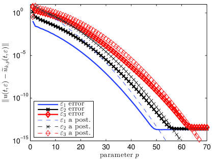
Figure 2: 2-norm errors of approximations $\widetilde{u}_{k,p}(t,\varepsilon)$ for the equation (5.4) and the error estimate (4.3) when $\varepsilon$ has the values $\varepsilon_{1}=1\cdot 10^{-3}$, $\varepsilon_{2}=1.5\cdot 10^{-2}$ and $\varepsilon_{3}=3\cdot 10^{-2}$.

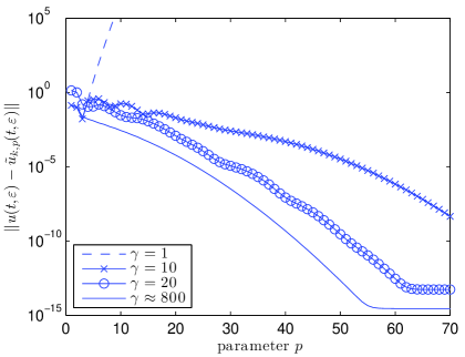
Figure 3: 2-norm errors of approximations $\widetilde{u}_{k,p}(t,\varepsilon)$, when $\varepsilon=1.5\cdot 10^{-2}$ using different scalings (5.1). The last option corresponds to the scaling (5.2).

5.3 Wave equation

Consider next the damped wave equation inside the 3D unit box given in [17, Section 5.2]. The governing $2n$-dimensional first-order differential equation is given by

(5.5) $$\frac{\hskip 1.0pt{\rm d}\hskip 0.5pt}{\hskip 1.0pt{\rm d}\hskip 0.5ptt}\begin{bmatrix}u(t)\\ u^{\prime}(t)\end{bmatrix}\begin{bmatrix}0&I\\ -M^{-1}K&-M^{-1}C(\gamma)\end{bmatrix}\begin{bmatrix}u(t)\\ u^{\prime}(t)\end{bmatrix},\quad\begin{bmatrix}u(0)\\ u^{\prime}(0)\end{bmatrix}=\begin{bmatrix}u_{0}\\ u_{0}^{\prime}\end{bmatrix}\in\mathbb{R}^{2n},$$

where $C(\gamma_{1},\gamma_{2})=\gamma_{1}C_{1}+\gamma_{2}C_{2}.$ The model is obtained by finite differences with 15 discretization points in each dimension, i.e., $n=15^{3}$. The matrix $K$ denotes the discretized Laplacian, $C(\gamma_{1},\gamma_{2})$ the damping matrix stemming from Robin boundary conditions, and $M$ the mass matrix. We carry out numerical experiments for parameter values $\gamma_{1}=0,1,2$ and $\gamma_{2}=0,1,2$.

We reformulate (5.5) in the form (1.1) by setting

$$A_{0}=\begin{bmatrix}0&I\\ -M^{-1}K&-M^{-1}\gamma_{1}C_{1}\end{bmatrix},\quad A_{1}=\begin{bmatrix}0&0\\ 0&-M^{-1}C_{2}\end{bmatrix}.$$

Then, the variable $\varepsilon$ in (1.1) corresponds to $\gamma_{2}$. This means that by running the algorithm for a fixed value of $\gamma_{1}$, we may efficiently obtain solutions for different values of $t$ and $\gamma_{2}$.

Figures 4 show the contour plots of the numerical solutions of (5.5) at $t=9$ on the plane $\{(x,y,z)\in[0,1]^{3}\,:\,z=0.5\}$ for different values of $(\gamma_{1},\gamma_{2})$. Note that for a fixed value of $\gamma_{1}$, only one run of the algorithm is required to compute the solution for many different $\gamma_{2}$.

In Figure 5 we illustrate the relative 2-norm errors of the approximations, when $\gamma_{1}=2$ and $\gamma_{2}=0,1$ and $2$. Then, $\|tA_{0}\|\approx 108$, and, respectively, $\|t\gamma_{2}A_{1}\|\approx 0,9.6$ and $12.9$. We again observe superlinear convergence, and, moreover, the a posteriori error estimate is very accurate for this example.

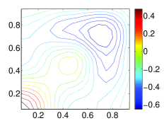
(a) $\gamma_{1}=\gamma_{2}=0$

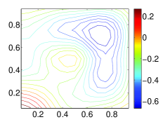
(b) $\gamma_{1}=1$, $\gamma_{2}=0$

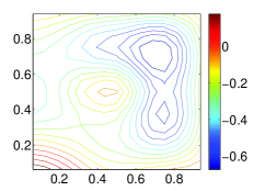
(c) $\gamma_{1}=2$, $\gamma_{2}=0$

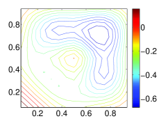
(d) $\gamma_{1}=1$, $\gamma_{2}=1$

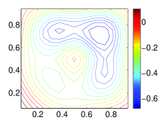
(e) $\gamma_{1}=1$, $\gamma_{2}=2$

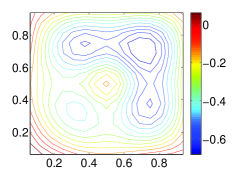
(f) $\gamma_{1}=2$, $\gamma_{2}=2$

Figure 4: The solution to (5.5) in the plane $z=0.5$, for different values of $(\gamma_{1},\gamma_{2})$ at $t=9$.

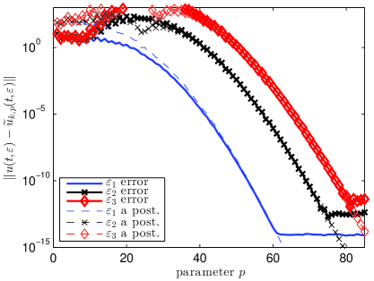
Figure 5: 2-norm errors of approximations $\widetilde{u}_{k,p}(t,\varepsilon)$ for the equation (5.4) and the error estimate (4.3), when $\gamma_{1}=2$ and $\gamma_{2}$ has the values $\varepsilon_{1}=1$, $\varepsilon_{2}=1.5$ and $\varepsilon_{3}=2$.

6 Conclusions and outlook

The focus of this paper is an algorithm for parameterized linear ODEs, which is shown to have superlinear convergence in theory and perform convincingly in several examples. The behavior is consistent with what is expected from an Arnoldi method. Due to the equivalence with the Arnoldi method, the algorithm may suffer from the typical disadvantages of the Arnoldi method, for instance, the fact that the computation time per iteration increases with the iteration number. The standard approach to resolve this issue is by using restarting, which we leave for future work.

Appendix A Technical lemmas for the norm and the field of values of $L_{m}$

We now provide bounds on the norm and the field of values of $L_{m}$, which are needed in Section 3.1. The derivation is done with properties of field of values. Recall that the field of values of a matrix $A\in\mathbb{C}^{n\times n}$ is defined as

$$\mathcal{F}(A)=\{x^{*}Ax\,:\,x\in\mathbb{C}^{n},\ \|x\|=1\}.$$

The bounds for the norm and the field of values of $\mathcal{A}_{N}$ follow from the block structure of $L_{m}$.

Lemma 8.

Let $N\geq 0$ and $L_{m}$ be given by (2.2). Then,

$$\|L_{m}\|\leq\sum\limits_{\ell=0}^{N}\|A_{\ell}\|$$

Proof.

Let $x=[x_{1}^{\mathrm{T}}\ \ldots\ x_{m}^{\mathrm{T}}]^{\mathrm{T}}\in\mathbb{C}^{nm}$ such that $x_{i}\in\mathbb{C}^{n}$ for all $1\leq i\leq m$ and $\|x\|=1$. From the block Toeplitz structure of $L_{m}$ we see that

$$\|L_{m}x\|\leq\sum\limits_{\ell=0}^{N}\sqrt{\sum\limits_{k=1}^{n-\ell}\|A_{\ell}x_{k}\|^{2}}\leq\sum\limits_{\ell=0}^{N}\|A_{\ell}\|\sqrt{\sum\limits_{k=1}^{n}\|x_{k}\|^{2}}=\sum\limits_{\ell=0}^{N}\|A_{\ell}\|.$$

∎

Next, we give a bound for the field of values of the matrix $L_{m}$. Let $d(\mathcal{S},z)$ denote the distance between a closed set $\mathcal{S}$ and a point $z$.

Lemma 9.

Let $N\geq 0$ and $L_{m}$ be given by (2.2). Then,

$$\mathcal{F}(L_{m})\subset\{z\in\mathbb{C}\,:\,d(\mathcal{F}(A_{0}),z)\leq\sum\limits_{\ell=1}^{N}\|A_{\ell}\|\}.$$

Proof.

Let $x=[x_{1}^{\mathrm{T}}\ \ldots\ x_{m}^{\mathrm{T}}]^{\mathrm{T}}\in\mathbb{C}^{nm}$, where $x_{i}\in\mathbb{C}^{n}$ for all $1\leq i\leq m$ and $\|x\|=1$. Then

(A.1) $$x^{*}L_{m}x=\sum\limits_{\ell=1}^{m}x_{\ell}^{*}A_{0}x_{\ell}+x^{*}\widetilde{L}_{m}x,$$

where $\widetilde{L}_{m}$ equals $L_{m}$ on the subdiagonal blocks and is otherwise zero. By the convexity of the field of values [14, Property 1.2.2], we know that $\sum_{\ell=1}^{m}x_{\ell}^{*}A_{0}x_{\ell}\in\mathcal{F}(A_{0})$. The second term in (A.1) can be bounded as in proof of Lemma 8, giving

$$|x^{*}\widetilde{L}_{m}x|\leq\|\widetilde{L}_{m}\|\leq\sum\limits_{\ell=1}^{N}\|A_{\ell}\|.$$

∎

As a corollary of Lemma 9, we have the following bound, which follows directly from the fact that the logarithmic norm of a matrix in 2-norm equals the real part of the rightmost point in its field of values.

Corollary 10.

Let $L_{m}$ be given by (2.2). Then,

(A.2) $$\mu(L_{m})\leq\mu(A_{0})+\sum\limits_{\ell=1}^{N}\|A_{\ell}\|,$$

where $\mu(A)$ denotes the logarithmic norm of $A$ defined in (1.5).

Appendix B Technical lemmas for coefficient bounds

We now derive bounds needed for the a priori analysis of the truncation error in Section 3.2. The following result provides an explicit characterization of the expansion coefficients. The proof technique is based on the same type of reasoning as what is commonly used in the analysis of Magnus series expansions for time-dependent ODEs; see, e.g., [5].

Lemma 11 (Explicit integral form).

Let $\ell$ and $N$ be positive integers such that $N\leq\ell$. Denote by $C_{\ell}$ the set of compositions of $\ell$, i.e.,

(B.1) $$C_{\ell}=\{(i_{1},\ldots,i_{r})\in\mathbb{N}_{+}^{r}\,:\,i_{1}+\cdots+i_{r}=\ell\},$$

and further denote

(B.2) $$C_{\ell,N}:=\{(i_{1},\ldots,i_{r})\in C_{\ell}\,:\,i_{s}\leq N\,\,\,\textrm{for all}\,\,\,1\leq s\leq r\}.$$

Then,

(B.3) $$c_{0}(t) ={\rm e}\hskip 1.0pt^{tA_{0}}u_{0},$$

$$c_{\ell}(t) =\sum\limits_{(i_{1},\ldots,i_{r})\in C_{\ell,N}}\int\limits_{0}^{t}{\rm e}\hskip 1.0pt^{(t-t_{i_{1}})A_{0}}A_{i_{1}}\int\limits_{0}^{t_{i_{1}}}{\rm e}\hskip 1.0pt^{(t_{i_{1}}-t_{i_{2}})A_{0}}A_{i_{2}}$$

$$\qquad\dots\int\limits_{0}^{t_{i_{r-1}}}{\rm e}\hskip 1.0pt^{(t_{i_{r-1}}-t_{i_{r}})A_{0}}A_{i_{r}}c_{0}(t_{i_{r}})\,\hskip 1.0pt{\rm d}\hskip 0.5ptt_{i_{1}}\ldots\hskip 1.0pt{\rm d}\hskip 0.5ptt_{i_{r}}\quad\textrm{for}\quad\ell>0.$$

Proof.

From the ODE (2.4) and the variation-of-constants formula it follows that

(B.4a) $$c_{0}(t) = {\rm e}\hskip 1.0pt^{tA_{0}}u_{0},$$

(B.4b) $$c_{\ell}(t) = \sum\limits_{k=1}^{\min\{N,\ell\}}\int\limits_{0}^{t}{\rm e}\hskip 1.0pt^{(t-s)A_{0}}A_{k}c_{\ell-k}(s)\,\hskip 1.0pt{\rm d}\hskip 0.5pts\qquad\textrm{for}\quad\ell>0.$$

Using (B.4) we now prove (B.3) by induction. For $\ell=1$, we have $C_{1}=\{(1)\}$ and $C_{1,1}=\{(1)\}$. From (B.4a) and (B.4b) we directly conclude that

$$c_{1}(t)=\int_{0}^{t}{\rm e}\hskip 1.0pt^{(t-t_{1})A_{0}}A_{1}c_{0}(t_{1})\,\hskip 1.0pt{\rm d}\hskip 0.5ptt_{1}.$$

Suppose (B.3) holds for $\ell=1,\ldots,p-1$ for some value $p>1$. From Definition (B.1), we know that the row sum of any element of $C_{p}$ is $p$, and the row sum of any element in $C_{p-k}$ is $p-k$. Therefore, $C_{p}$ satisfies the recurrence relation

(B.5) $$C_{p}=\bigcup_{k=1}^{p}\;\bigcup_{(i_{1},\ldots,i_{r})\in C_{p-k}}\;\;(k,i_{1},\ldots,i_{r})$$

and

(B.6) $$C_{p,N}=\bigcup_{k=1}^{\min(N,p)}\;\bigcup_{(i_{1},\ldots,i_{r})\in C_{p-k,N}}\;\;(k,i_{1},\ldots,i_{r}).$$

By using (B.4b) with $\ell=p$ and the fact that (B.3) is assumed to be satisfied for $\ell=1,\ldots,p-1$ we have

$$c_{p}(t)= \sum\limits_{k=1}^{\min\{N,p\}}\int\limits_{0}^{t}{\rm e}\hskip 1.0pt^{(t-s)A_{0}}A_{k}c_{p-k}(s)\,\hskip 1.0pt{\rm d}\hskip 0.5pts$$

$$=\sum\limits_{k=1}^{\min\{N,p\}}\int\limits_{0}^{t}{\rm e}\hskip 1.0pt^{(t-s)A_{0}}A_{k}\sum\limits_{(i_{1},\ldots,i_{r})\in C_{p-k,N}}\int\limits_{0}^{s}{\rm e}\hskip 1.0pt^{(s-t_{i_{1}})A_{0}}A_{i_{1}}\dots$$

$$\qquad\int\limits_{0}^{t_{i_{r-1}}}{\rm e}\hskip 1.0pt^{(t_{i_{r-1}}-t_{i_{r}})A_{0}}A_{i_{r}}c_{0}(t_{i_{r}})\hskip 1.0pt{\rm d}\hskip 0.5ptt_{i_{1}}\ldots\hskip 1.0pt{\rm d}\hskip 0.5ptt_{i_{r}}\hskip 1.0pt{\rm d}\hskip 0.5pts.$$

By rearranging the terms as a double sum and using (B.6), we have

$$c_{p}(t) =\sum\limits_{k=1}^{\min\{N,p\}}\sum\limits_{(i_{1},\ldots,i_{r})\in C_{p-k,N}}\int\limits_{0}^{t}{\rm e}\hskip 1.0pt^{(t-s)A_{0}}A_{k}\int\limits_{0}^{s}{\rm e}\hskip 1.0pt^{(s-t_{i_{1}})A_{0}}A_{i_{1}}\dots$$

$$\quad\quad\int\limits_{0}^{t_{i_{r-1}}}{\rm e}\hskip 1.0pt^{(t_{i_{r-1}}-t_{i_{r}})A_{0}}A_{i_{r}}c_{0}(t_{i_{r}})\hskip 1.0pt{\rm d}\hskip 0.5ptt_{i_{1}}\ldots\hskip 1.0pt{\rm d}\hskip 0.5ptt_{i_{r}}\hskip 1.0pt{\rm d}\hskip 0.5pts$$

$$=\sum\limits_{(i_{1},\ldots,i_{r})\in C_{p,N}}\int\limits_{0}^{t}{\rm e}\hskip 1.0pt^{(t-t_{i_{1}})A_{0}}A_{i_{1}}\dots\int\limits_{0}^{t_{i_{r-1}}}{\rm e}\hskip 1.0pt^{(t_{i_{r-1}}-t_{i_{r}})A_{0}}A_{i_{r}}c_{0}(t_{i_{r}})\hskip 1.0pt{\rm d}\hskip 0.5ptt_{i_{1}}\ldots\hskip 1.0pt{\rm d}\hskip 0.5ptt_{i_{r}}$$

which shows that (B.3) holds for $\ell=p$ and completes the proof.

∎

Lemma 12.

Let $m,N$ be positive integers, $N\leq m$, and let $C_{m,N}$ be defined as in (B.2). Let $(i_{1},i_{2},\ldots,i_{r})\in C_{m,N}$, $a=\max_{j=1,\dots,N}\|A_{j}\|$, and assume that for all $1\leq j\leq N$. Then, one corresponding term in (B.3) is bounded as

(B.7) $$\quad\|\int\limits_{0}^{t}{\rm e}\hskip 1.0pt^{(t-t_{i_{1}})A_{0}}A_{i_{1}}\ldots\int\limits_{0}^{t_{i_{r-1}}}{\rm e}\hskip 1.0pt^{(t_{i_{r-1}}-t_{i_{r}})A_{0}}A_{i_{r}}c_{0}(t_{i_{r}})\,\hskip 1.0pt{\rm d}\hskip 0.5ptt_{i_{1}}\ldots\hskip 1.0pt{\rm d}\hskip 0.5ptt_{i_{r}}\|$$

$$\qquad\leq{\rm e}\hskip 1.0pt^{t\mu(A_{0})}\frac{(ta)^{r}}{r!}\|u_{0}\|.$$

Proof.

By using the Dahlquist bound [22, p. 138] for the matrix exponential, the rightmost integral on the left-hand side of (B.7) can be bounded as

$$\|\int\limits_{0}^{t_{i_{r-1}}}{\rm e}\hskip 1.0pt^{(t_{i_{r-1}}-t_{i_{r}})A_{0}}A_{i_{r}}{\rm e}\hskip 1.0pt^{t_{i_{r}}A_{0}}u_{0}\,\hskip 1.0pt{\rm d}\hskip 0.5ptt_{i_{r}}\|$$

$$\leq \int\limits_{0}^{t_{i_{r-1}}}{\rm e}\hskip 1.0pt^{(t_{i_{r-1}}-t_{i_{r}})\mu(A_{0})}\|A_{i_{r}}\|{\rm e}\hskip 1.0pt^{{t_{i_{r}}}\mu(A_{0})}\hskip 1.0pt{\rm d}\hskip 0.5ptt_{i_{r}}\|u_{0}\|=t_{i_{r-1}}a{\rm e}\hskip 1.0pt^{t_{i_{r-1}}\mu(A_{0})}\,\|u_{0}\|.$$

The claim (B.7) follows by applying the same bounding technique $r-1$ times for the remaining integrals, and using that $t_{i}\leq t$ for any $i$. ∎

Lemma 13 (Coefficient bound).

Let $c_{0}$,$c_{1}$,…be the $\varepsilon$-expansion of $u(t,\varepsilon)$ in (1.2) for $N\geq 1$ in (1.2), and let $a=\max_{j=1,\dots,N}\|A_{j}\|$. Then, for any $\ell\geq 0$ such that $k:=\lceil\frac{\ell}{N}\rceil\geq 2$,

$$\|c_{\ell}(t)\|\leq{\rm e}\hskip 1.0pt^{t(\mu(A_{0})+{\rm e}\hskip 1.0ptNa)-1}\frac{({\rm e}\hskip 1.0ptNta)^{k}}{(k-1)!}\|u_{0}\|.$$

Proof.

We first note that the maximum length of any vector in $C_{m,N}$ is $m$, and the vector with the shortest length has length at least $k=\lceil\frac{m}{N}\rceil$. Hence, Lemma 11 can be rephrased as

(B.8) $$c_{m}(t) =\sum\limits_{\widehat{r}=k}^{m}\ \underset{r=\widehat{r}}{\sum\limits_{(i_{1},\ldots,i_{r})\in C_{m,N}}}\int\limits_{0}^{t}{\rm e}\hskip 1.0pt^{(t-t_{i_{1}})A_{0}}A_{i_{1}}$$

$$\qquad\dots\int\limits_{0}^{t_{i_{r-1}}}{\rm e}\hskip 1.0pt^{(t_{i_{r-1}}-t_{i_{r}})A_{0}}A_{i_{r}}c_{0}(t)\,\hskip 1.0pt{\rm d}\hskip 0.5ptt_{i_{1}}\ldots\hskip 1.0pt{\rm d}\hskip 0.5ptt_{i_{r}}.$$

Since, $C_{m,N}\subset C_{m}$ we can bound the number of elements in $C_{m,N}$

$$\#\{(i_{1},\ldots,i_{r})\in C_{m,N}\,:\,r=\ell\}\leq\#\{(i_{1},\ldots,i_{r})\in C_{m}\,:\,r=\ell\}=\binom{m-1}{\ell-1},$$

and Lemma 12 and (B.8) imply that

$$\|c_{m}(t)\|\leq{\rm e}\hskip 1.0pt^{t\mu(A_{0})}\sum\limits_{\ell=k}^{m}\binom{m-1}{\ell-1}\frac{(ta)^{\ell}}{\ell!}\|u_{0}\|.$$

Moreover,

$$\binom{m-1}{r-1} =\frac{(m-1)(m-2)\cdots(m-r+1)}{(r-1)!}\leq\frac{m^{r}}{(r-1)!}$$

and therefore

(B.9) $$\|c_{m}(t)\|\leq{\rm e}\hskip 1.0pt^{t\omega(A_{0})}\sum\limits_{r=k}^{m}\frac{m^{r}(ta)^{r}}{(r-1)!\,r!}\|u_{0}\|\leq{\rm e}\hskip 1.0pt^{t\mu(A_{0})}\sum\limits_{r=k}^{m}\frac{r^{r}(Nta)^{r}}{(r-1)!\,r!}\|u_{0}\|.$$

In the second inequality in (B.9) we use $m=N\frac{m}{N}\leq N\lceil\frac{m}{N}\rceil=Nk\leq Nr$. Using the inequality ${\rm e}\hskip 1.0pt\left(\frac{n}{{\rm e}\hskip 1.0pt}\right)^{n}\leq n!$, $n\geq 1$, we see that for $k\geq 2$

$$\|c_{m}(t)\| \leq{\rm e}\hskip 1.0pt^{t\mu(A_{0})}\sum\limits_{r=k}^{m}\frac{r^{r}(Nta)^{r}}{{\rm e}\hskip 1.0pt\left(\frac{r}{{\rm e}\hskip 1.0pt}\right)^{r}(r-1)!}\|u_{0}\|\leq{\rm e}\hskip 1.0pt^{t\mu(A_{0})}\sum\limits_{r=k}^{\infty}\frac{({\rm e}\hskip 1.0ptNta)^{r}}{{\rm e}\hskip 1.0pt(r-1)!}\|u_{0}\|$$

$$={\rm e}\hskip 1.0pt^{t\mu(A_{0})-1}({\rm e}\hskip 1.0ptNta)^{k}\sum_{r=0}^{\infty}\frac{r!}{(r+k-1)!}\frac{({\rm e}\hskip 1.0ptNta)^{r}}{r!}\|u_{0}\|$$

$$\leq\frac{{\rm e}\hskip 1.0pt^{t(\mu(A_{0})+{\rm e}\hskip 1.0ptNa)-1}({\rm e}\hskip 1.0ptNta)^{k}}{(k-1)!}\|u_{0}\|,$$

where in the last inequality we use $\frac{r!}{(r+k-1)!}\leq\frac{1}{(k-1)!}$. ∎

References

- [1] A. H. Al-Mohy and N. J. Higham. Computing the action of the matrix exponential, with an application to exponential integrators. SIAM J. Sci. Comput., 33:488–511, 2011.
- [2] A. Antoulas, D. Sorensen, and S. Gugercin. A survey of model reduction methods for large-scale systems. Contemporary Mathematics, 280:193–220, 2006.
- [3] P. Benner, S. Gugercin, and K. Willcox. A survey of model reduction methods for parametric systems. Technical report, Max Planck Institute Magdeburg, 2013.
- [4] T. Betcke. Optimal scaling of generalized and polynomial eigenvalue problems. SIAM J. Matrix Anal. Appl., 30(4):1320–1338, 2008.
- [5] S. Blanes, F. Casas, J. Oteo, and J. Ros. The Magnus expansion and some of its applications. Physics Reports, 470:151–238, 2009.
- [6] R. Eid. Time Domain Model Reduction By Moment Matching. PhD thesis, TU München, 2008.
- [7] H.-Y. Fan, W.-W. Lin, and P. Van Dooren. Normwise scaling of second order polynomial matrices. SIAM J. Matrix Anal. Appl., 26(1):252–256, 2004.
- [8] E. Gallopoulos and Y. Saad. Efficient solution of parabolic equations by Krylov approximation methods. SIAM J. Sci. Stat. Comput., 13(5):1236–1264, 1992.
- [9] N. J. Higham. Functions of Matrices. Theory and Computation. SIAM, 2008.
- [10] N. J. Higham and S. D. Relton. Higher order Fréchet derivatives of matrix functions and the level-2 condition number. SIAM J. Matrix Anal. Appl., 35(3):1019–1037, 2014.
- [11] M. Hochbruck and C. Lubich. On Krylov subspace approximations to the matrix exponential operator. SIAM J. Numer. Anal., 34(5):1911–1925, 1997.
- [12] M. Hochbruck, C. Lubich, and H. Selhofer. Exponential integrators for large systems of differential equations. SIAM J. Sci. Comput., 19(5):1552–1574, 1998.
- [13] M. Hochbruck and A. Ostermann. Exponential integrators. Acta Numerica, 19:209–286, 2010.
- [14] R. Horn and C. Johnson. Topics in Matrix Analysis. Cambridge University Press, Cambridge, UK, 1991.
- [15] E. Jarlebring, W. Michiels, and K. Meerbergen. A linear eigenvalue algorithm for the nonlinear eigenvalue problem. Numer. Math., 122(1):169–195, 2012.
- [16] A. Koskela and E. Jarlebring. The infinite Arnoldi exponential integrator for linear inhomogeneous ODEs. Technical report, KTH Royal institute of technology, 2014. arxiv preprint.
- [17] P. Lietaert and K. Meerbergen. Interpolatory model order reduction by tensor Krylov methods. Technical report, KU Leuven, 2015.
- [18] R. Mathias. A chain rule for matrix functions and applications. SIAM J. Matrix Anal. Appl., 17(3):610–620, 1996.
- [19] I. Najfeld and T. F. Havel. Derivatives of the matrix exponential and their computation. Adv. Appl. Math., 16(3):321–375, 1995.
- [20] S. D. Relton. Algorithms for Matrix Functions and their Fréchet Derivatives and Condition Numbers. PhD thesis, Univ. Manchester, 2014.
- [21] Y. Saad. Analysis of some Krylov subspace approximations to the matrix exponential operator. SIAM J. Numer. Anal., 29(1):209–228, 1992.
- [22] L. N. Trefethen and M. Embree. Spectra and Pseudospectra. The Behavior of Nonnormal Matrices and Operators. Princeton University Press, 2005.
- [23] Y. Yue and K. Meerbergen. Using Krylov-Padé model order reduction for accelerating design optimization of structures and vibrations in the frequency domain. Int. J. Numer. Methods Eng., 90(10):1207–1232, 2012.