A perturbed lepton-specific two-Higgs-doublet model facing experimental hints for physics beyond the Standard Model

Abstract

The BaBar, Belle, and LHCb collaborations have reported evidence for new physics in $B\to D\tau\nu$ and $B\to D^{*}\tau\nu$ of approximately $3.8\sigma$. There is also the long lasting discrepancy of about $3\sigma$ in the anomalous magnetic moment of the muon, and the branching ratio for $\tau\to\mu\nu\nu$ is $1.8\sigma$ ($2.4\sigma$) above the Standard Model expectation using the HFAG (PDG) values. Furthermore, CMS found hints for a non-zero decay rate of $h\to\mu\tau$. Interestingly, all these observations can be explained by introducing new scalars. In this article we consider these processes within a lepton-specific two-Higgs doublet model (i.e. of type X) with additional non-standard Yukawa couplings. It is found that one can accommodate $\tau\to\mu\nu\nu$ with modified Higgs–$\tau$ couplings. The anomalous magnetic moment of the muon can be explained if the additional neutral CP-even Higgs $H$ is light (below 100 GeV). Also ${\cal R}(D)$ and ${\cal R}(D^{*})$ can be easily explained by additional $t$–$c$–Higgs couplings. Combining these $t$–$c$ couplings with a light $H$ the decay rate for $t\to Hc$ can be in a testable range for the LHC. Effects in $h\to\mu\tau$ are also possible, but in this case a simultaneous explanation of the anomalous magnetic moment of the muon is difficult due to the unavoidable $\tau\to\mu\gamma$ decay.

I Introduction

In addition to direct searches for new physics (NP) performed at very high energies at the LHC, low-energy precision flavour observables provide a complementary window to physics beyond the Standard Model (SM). Here, the anomalous magnetic moment of the muon $(g-2)_{\mu}$ is a prime example as it is very sensitive to physics beyond the SM entering via quantum corrections. Also, tauonic $B$ meson decays and $\tau\to\mu\nu\nu$ are excellent probes of NP: they test lepton flavour universality – satisfied in the SM – and are sensitive to new degrees of freedom that couple proportional to the mass of the involved particles (e.g. Higgs bosons Krawczyk and Pokorski (1988)) because of the heavy $\tau$ lepton involved. The observation of flavour violating decays of the SM Higgs, most importantly $h\to\mu\tau$, would prove the existence of physics beyond the SM.

Let us briefly review the current experimental and theoretical situation in these processes. The world average of the measurement of $a_{\mu}\equiv(g-2)_{\mu}/2$ is completely dominated by the Brookhaven experiment E821 Bennett et al. (2006) and is given by Olive et al. (2014)

$$a_{\mu}^{\mathrm{exp}}=(116\,592\,091\pm 54\pm 33)\times 10^{-11}\,,$$ (1)

where the first error is statistical and the second systematic. The current SM prediction is

$$a_{\mu}^{\mathrm{SM}}=(116\,591\,855\pm 59)\times 10^{-11}\,,$$ (2)

where almost the whole uncertainty is due to hadronic effects. This amounts to a discrepancy between the SM and experimental value of $a_{\mu}^{\mathrm{exp}}-a_{\mu}^{\mathrm{SM}}=(236\pm 87)\times 10^{-11}$, i.e. a $2.7\sigma$ deviation. It is not yet clear if this discrepancy is due to NP or rather underestimated hadronic uncertainties; there are ongoing efforts to reduce the model dependence in the hadronic light-by-light estimate based on dispersion relations Colangelo et al. (2014b, c); Colangelo et al. (2015) or lattice QCD Hayakawa et al. (2006); Blum et al. (2012, 2015); Green et al. (2015). Possible NP explanations besides supersymmetry (see for example Ref. Stöckinger (2007) for a review) include very light $Z^{\prime}$ bosons Langacker (2009); Baek et al. (2001); Ma et al. (2002); Gninenko and Krasnikov (2001); Pospelov (2009); Heeck and Rodejohann (2011); Harigaya et al. (2014); Altmannshofer et al. (2014), leptoquarks Chakraverty et al. (2001); Cheung (2001), additional fermions Freitas et al. (2014) but also new scalar contributions in two-Higgs-doublet models (2HDM) Iltan and Sundu (2003); Omura et al. (2015), also within the lepton-specific 2HDM Broggio et al. (2014); Wang and Han (2015); Abe et al. (2015).

Concerning tauonic $B$ decays, the BaBar collaboration performed an analysis of the semileptonic $B$ decays $B\to D\tau\nu$ and $B\to D^{*}\tau\nu$ using the full available data set Lees et al. (2012a). Recently, these decays have also been reanalyzed by Belle Chur (2015); Huschle et al. (2015), and LHCb measured the mode $B\to D^{*}\tau\nu$ Aaij et al. (2015). These experiments find for the ratios

$${\cal R}(D^{(*)})\,\equiv\,\frac{{\rm BR}(B\to D^{(*)}\tau\nu)}{{\rm BR}(B\to D^{(*)}\ell\nu)}\,,$$ (3)

where $\ell=e$ or $\mu$, the following values:

$$\begin{split}{\cal R}(D)_{\rm BABAR}\,&=\,0.440\pm 0.058\pm 0.042\,,\\ {\cal R}(D)_{\rm BELLE}\,&=\,0.375\pm 0.064\pm 0.026\,,\\ {\cal R}(D^{*})_{\rm BABAR}\,&=\,0.332\pm 0.024\pm 0.018\,,\\ {\cal R}(D^{*})_{\rm BELLE}\,&=\,0.293\pm 0.038\pm 0.015\,,\\ {\cal R}(D^{*})_{\rm LHCb}\,&=\,0.336\pm 0.027\pm 0.030\,.\end{split}$$ (4)

Here, the first error is statistical and the second one is systematic. Combining these measurements one finds Rotondo (2015)

$$\begin{split}{\cal R}(D)_{\rm exp}\,&=\,0.388\pm 0.047\,,\\ {\cal R}(D^{*})_{\rm exp}\,&=\,0.321\pm 0.021\,.\end{split}$$ (5)

Comparing the experimental values to the SM prediction

$$\begin{split}{\cal R}(D)_{\rm SM}\,&=\,0.297\pm 0.017\,,\\ {\cal R}(D^{*})_{\rm SM}\,&=\,0.252\pm 0.003\,,\end{split}$$ (6)

we see that there is a discrepancy of 1.8$\sigma$ for ${\cal R}(D)$ and 3.3$\sigma$ for ${\cal R}(D^{*})$; combining them gives a $3.8\sigma$ deviation from the SM (compared to $3.4\sigma$ taking into account the BaBar results only Lees et al. (2012b)). Models solving the ${\cal R}(D)$ puzzle have been discussed extensively in the literature Fajfer et al. (2012b); Crivellin et al. (2012); Datta et al. (2012); Celis et al. (2013); Crivellin et al. (2013); Li et al. (2014); Faisel (2014); Atoui et al. (2014); Sakaki et al. (2013); Doršner et al. (2013); Biancofiore et al. (2014); Alonso et al. (2015); Greljo et al. (2015); Calibbi et al. (2015); Freytsis et al. (2015), including the possibility of charged Higgs particles Crivellin et al. (2012); Celis et al. (2013); Crivellin et al. (2013).

For $\tau\to\mu\nu\nu$, the dominant uncertainty in the SM prediction for the branching ratio comes from the $\tau$ lifetime $\tau_{\tau}$. Using the PDG Olive et al. (2014) values for $\tau$ lifetime, $\tau_{\tau}=(290.3\pm 0.5)\times 10^{-15}\,\mathrm{s}$, and branching ratios

$$\begin{split}B_{\mu}&\equiv{\rm BR}(\tau\to\mu\overline{\nu}\nu)_{\mathrm{exp}}=(17.41\pm 0.04)\%\,,\\ B_{e}&\equiv{\rm BR}(\tau\to e\overline{\nu}\nu)_{\mathrm{exp}}=(17.83\pm 0.04)\%\,,\end{split}$$ (7)

we can determine the deviations $\Delta_{\ell}\equiv B_{\ell}/B_{\ell}^{\mathrm{SM}}-1$ Krawczyk and Temes (2005) from the SM prediction to be

$$\Delta_{\mu}^{\rm PDG}=(0.69\pm 0.29)\%\,, \Delta_{e}=(0.28\pm 0.28)\%\,.$$ (8)

There is a deviation of about $2.4\sigma$ in the muon data, whereas the electron channel is compatible with the SM prediction. HFAG finds essentially the same value for the tau lifetime, but a slightly lower ${\rm BR}(\tau\to\mu\overline{\nu}\nu)_{\mathrm{exp}}=(17.39\pm 0.04)\%$ Amhis et al. (2014), alleviating the deviation to approximately $2\sigma$:

$$\Delta_{\mu}^{\rm HFAG}=(0.59\pm 0.32)\%\,.$$ (9)

Again, charged Higgses Hollik and Sack (1992); Krawczyk and Temes (2005); Aoki et al. (2009) but also neutral $Z^{\prime}$ bosons Crivellin et al. (2015a) affect this decay.

Moving from lepton non-universality to outright lepton flavour violation, we are drawn to the recent CMS excess of $2.4\sigma$ in $h\to\mu\tau$ Khachatryan et al. (2015):

$${\rm BR}(h\to\mu\tau)=\left(0.84_{-0.37}^{+0.39}\right)\%\,.$$ (10)

Possible explanations naturally require an extended Higgs sector Campos et al. (2015); Aristizabal Sierra and Vicente (2014); Heeck et al. (2015); Crivellin et al. (2015b); Dorsner et al. (2015); Omura et al. (2015); Crivellin et al. (2015c).

As we see from the previous discussion, all discrepancies outlined above can be solved by additional scalar bosons. In the simplest extension of the SM with additional charged Higgses, a 2HDM, one introduces a second Higgs doublet and obtains four additional physical Higgs particles (in the case of a CP conserving Higgs potential): the neutral CP-even Higgs $H$, a neutral CP-odd Higgs $A$ and the two charged Higgses $H^{\pm}$. 2HDMs have been studied for many years with focus on the type-II models Miki et al. (2002); Wahab El Kaffas et al. (2007); Deschamps et al. (2010). However, there are also other models without flavour-changing neutral currents at tree-level, i.e. type-I, type-X (lepton-specific) and the flipped 2HDM (see Ref. Branco et al. (2012) for an review). More general models with flavour-changing neutral Higgs couplings at tree-level are named type-III models. Here the focus has been on minimal flavour violation D’Ambrosio et al. (2002); Buras et al. (2010); Blankenburg and Isidori (2012), alignment Pich and Tuzon (2009); Jung et al. (2010) or natural flavour conservation Glashow and Weinberg (1977); Buras et al. (2010) but also generic 2HDMs of type III have been studied Crivellin et al. (2013). In these models type II is recovered in the absence of flavour-changing neutral Higgs couplings. While the type-II model cannot explain ${\cal R}(D)$ and ${\cal R}(D^{*})$ simultaneously Lees et al. (2012a), this can be achieved by supplementing the model with additional non-holomorphic couplings Crivellin et al. (2012). However, this model (as the normal type-II model) is under pressure from $b\to s\gamma$ data Misiak et al. (2015) and LHC searches for $A\to\tau\tau$ Khachatryan et al. (2014). Furthermore, no sizable effect in the anomalous magnetic moment of the muon can be generated Crivellin et al. (2013) and also explaining $h\to\mu\tau$ is challenging.

Therefore, we choose to consider in this article the 2HDM of type X (lepton-specific). In this model the heavy Higgs couplings to quarks are suppressed compared to the type-II model and the bounds from $b\to s\gamma$ and LHC searches are much weaker, leaving more space for effects in $(g-2)_{\mu}$ and tauonic $B$ decays. Furthermore, the sign of the coupling of heavy Higgses to the $\tau$ lepton can be reversed, allowing for constructive interference in $\tau\to\mu\nu\nu$. Also, large effects in $h\to\mu\tau$ compared to the type-II-like model are possible as the Barr-Zee contributions to $\tau\to\mu\gamma$ involving quarks are suppressed.

The article is structured as follows: in the next section we outline our model, i.e. the 2HDM of type X with additional non-standard Yukawa couplings. Sec. 3 discusses the relevant observables and collects the necessary formulae. Sec. 4 contains the numerical analysis. Finally we conclude in Sec. 5.

II 2HDM-X

We will study a lepton-specific 2HDM (2HDM-X), defined by the Yukawa couplings in the Lagrangian

$$\mathcal{L}_{Y}=-\overline{Q}_{L}Y^{u}\tilde{\Phi}_{2}u_{R}-\overline{Q}_{L}Y^{d}\Phi_{2}d_{R}-\overline{L}_{L}Y^{\ell}\Phi_{1}e_{R}+\mathrm{h.c.}\,,$$ (11)

with additional couplings that break the type-X structure

$$\Delta\mathcal{L}_{Y}=-\overline{Q}_{L}\xi^{u}\tilde{\Phi}_{1}u_{R}-\overline{Q}_{L}\xi^{d}\Phi_{1}d_{R}-\overline{L}_{L}\xi^{\ell}\Phi_{2}e_{R}+\mathrm{h.c.}$$ (12)

For arbitrary matrices $Y^{u,d,\ell}$ and $\xi^{u,d,\ell}$ this simply parametrizes the 2HDM with the most general Yukawa interactions (type III). We will however assume the coupling structure to be close to type X, i.e. the $\xi$ matrices to be small perturbations. After electroweak symmetry breaking the following field redefinitions are necessary in order to render the fermion mass matrices diagonal

$$\begin{array}[]{l}{d_{L,R}}\to D_{L,R}^{\dagger}{d_{L,R}}\,,\\ {u_{L,R}}\to U_{L,R}^{\dagger}{u_{L,R}}\,,\\ {\ell_{L,R}}\to L_{L,R}^{\dagger}{\ell_{L,R}}\,.\end{array}$$ (13)

We define the (non-diagonal) coupling matrices

$$\epsilon^{u}\equiv U_{L}^{\dagger}\xi^{u}U_{R}\,, \epsilon^{d}\equiv D_{L}^{\dagger}\xi^{d}D_{R}\,, \epsilon^{\ell}\equiv L_{L}^{\dagger}\xi^{\ell}L_{R}\,,$$ (14)

and express the Yukawa couplings in terms of the physical masses and the couplings $\epsilon$. Note that we are not concerned with the issue of neutrino masses in this article, and hence do not introduce e.g. right-handed neutrinos. Therefore, the Higgs interactions with fermions can be written as

$$\begin{split}\mathcal{L}\ &\supset\ {{\bar{\nu}}_{i}}\Gamma_{{\nu_{i}}{\ell_{j}}}^{{H^{+}}\;LR}{P_{R}}{\ell_{j}}{H^{+}}\\ &\quad+{{\bar{u}}_{i}}\left({\Gamma_{{u_{i}}{d_{j}}}^{{H^{+}}\;RL}{P_{L}}+\Gamma_{{u_{i}}{d_{j}}}^{{H^{+}}\;LR}{P_{R}}}\right){d_{j}}{H^{+}}{\mkern 1.0mu}\\ &\quad+\sum\limits_{H_{k}^{0}={h},{A},{H}}{\sum\limits_{f=u,d,\ell}{\left({{{\bar{f}}_{i}}\,\Gamma_{{f_{i}}{f_{j}}}^{H_{k}^{0}\;LR}\,{P_{R}}{f_{j}}{\mkern 1.0mu}H_{k}^{0}}\right)}}+\mathrm{h.c.}\,,\end{split}$$ (15)

where the couplings are given by

$$\Gamma_{{q_{i}}{q_{j}}}^{{h}LR} \simeq-\frac{1}{\sqrt{2}}\left(\frac{{{m_{{q_{i}}}}}}{v}{\delta_{ij}}\cos\alpha-\epsilon_{ij}^{q}\sin\alpha\right),$$ (16)

$$\Gamma_{{q_{i}}{q_{j}}}^{{H}LR} \simeq-\frac{1}{\sqrt{2}}\left(\frac{{{m_{{q_{i}}}}}}{v}{\delta_{ij}}\sin\alpha+\epsilon_{ij}^{q}\cos\alpha\right),$$ (17)

$$\Gamma_{{d_{i}}{d_{j}}}^{{A}LR} \simeq-i\frac{1}{{\sqrt{2}}}\epsilon_{ij}^{d}\,,$$ (18)

$$\Gamma_{{u_{i}}{u_{j}}}^{{A}LR} \simeq i\frac{1}{{\sqrt{2}}}\epsilon_{ij}^{u}\,,$$ (19)

$$\Gamma_{{u_{i}}{d_{j}}}^{{H^{+}}LR} \simeq{V_{ij^{\prime}}}\epsilon_{j^{\prime}j}^{d}\,,$$ (20)

$$\Gamma_{{u_{i}}{d_{j}}}^{{H^{+}}RL} \simeq-\epsilon_{j^{\prime}i}^{u*}{V_{j^{\prime}j}}\,,$$ (21)

$$\Gamma_{{\ell_{f}}{\ell_{i}}}^{{h}LR{\kern 1.0pt}} \simeq\frac{\sin\alpha\tan\beta}{\sqrt{2}}\left({\frac{{{m_{{\ell_{i}}}}}}{v}{\delta_{fi}}-{\epsilon_{fi}^{\ell}}}\right)\,,$$ (22)

$$\Gamma_{{\ell_{f}}{\ell_{i}}}^{{H}LR} \simeq-\frac{\cos\alpha\tan\beta}{\sqrt{2}}\left({\frac{{{m_{{\ell_{i}}}}}}{v}{\delta_{fi}}-{\epsilon_{fi}^{\ell}}}\right){\mkern 1.0mu}\,,$$ (23)

$$\Gamma_{{\ell_{f}}{\ell_{i}}}^{{A}LR} \simeq-i\frac{\tan\beta}{\sqrt{2}}\left({\frac{{{m_{{\ell_{i}}}}}}{v}\;{\delta_{fi}}-{\epsilon_{fi}^{\ell}}}\right)\,,$$ (24)

$$\Gamma_{{\nu_{f}}{\ell_{i}}}^{{H^{+}}LR{\kern 1.0pt}} \simeq\tan\beta\left({\frac{{{m_{{\ell_{i}}}}}}{v}{\delta_{fi}}-{\epsilon_{fi}^{\ell}}}\right)\,,$$ (25)

in the limit of large $\tan\beta$ of interest in this article. $V\equiv U_{L}^{\dagger}D_{L}$ denotes the Cabibbo–Kobayashi–Maskawa (CKM) mixing matrix and $v\simeq 174\,\mathrm{GeV}$ the vacuum expectation value. Note that for $\epsilon^{\ell}_{33}>m_{\tau}/v$ the sign of the couplings of $A$, $H$ and $H^{+}$ to taus is reversed. This will be important later as in this way the sign of the contribution to $\tau\to\mu\nu\nu$ can be flipped. In our notation, $h$ is the SM-like Higgs, $H$ and $A$ are the additional CP-even and CP-odd Higges; due to the mainly leptophilic couplings of $H$ and $A$, collider bounds on their masses are quite weak and they can be even lighter than the SM-like scalar boson. In particular, $\sin(\beta-\alpha)=1$ always corresponds to the SM-like limit, even for $m_{H}<m_{h}$ (this differs from standard 2HDM literature).

In the following, we will assume $\epsilon^{d}=0$ for simplicity, as it is stringently constrained from FCNC processes Crivellin et al. (2013). In addition, we take $\epsilon^{u}$ to be of the form

$$\epsilon^{u}=\begin{pmatrix}0&0&0\\ 0&0&0\\ 0&\times&\times\end{pmatrix},$$ (26)

where $\times$ denotes a non-zero entry, since again $\epsilon^{u}_{13}$ ($\epsilon^{u}_{23}$) is severely constrained from $b\to d(s)\gamma$ Crivellin and Mercolli (2011). In the lepton sector we take the same structure as for the $\epsilon^{u}$:

$$\epsilon^{\ell}=\begin{pmatrix}0&0&0\\ 0&0&0\\ 0&\times&\times\end{pmatrix}.$$ (27)

In this way we avoid lepton flavour violation involving electrons (i.e. bounds from $\mu\to e\gamma$, $\mu\to eee$ and $\mu\to e$ conversion in nuclei), but still allow for effects in $\Delta a_{\mu}$, $\tau\to\mu\nu\nu$, and even $h\to\mu\tau$.

We will not attempt to find a symmetry realisation of the $\epsilon^{f}$ structures, but take them merely as a convenient minimal set of parameters to explain existing anomalies. Should the above structures prove successful, one might try to find appropriate flavour symmetries to generate them dynamically.

III Observables

In this section we discuss the relevant processes and summarize the formulae needed for the phenomenological analysis.

III.1 Tauonic $B$ decays

In a 2HDM of type II the charged Higgs contribution to $B\to\tau\nu$ Hou (1993), ${\cal R}(D)$ and ${\cal R}(D^{*})$ interferes necessarily destructively with the SM and, in addition, ${\cal R}(D)$ and ${\cal R}(D^{*})$ cannot be explained simultaneously Lees et al. (2012a). However, an enhancement is possible in type-III models, see Ref. Crivellin et al. (2012). We do not discuss $B\to\tau\nu$ here, which depends on the value of $V_{ub}$. If the inclusive value is taken for $V_{ub}$, it agrees well with the SM prediction, but it is above the SM value if the exclusive determination is used. (Note that the differences between the inclusive and exclusive determination cannot be explained by NP Crivellin and Pokorski (2015).)

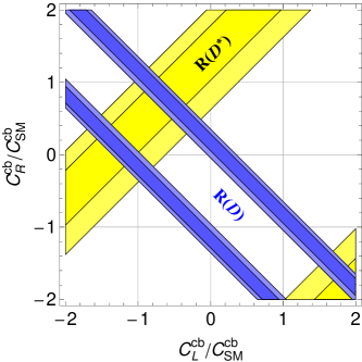
Figure 1: Allowed regions in the $C^{L}_{23}$-$C^{R}_{23}$ plane from ${\cal R}(D)$ (blue) and ${\cal R}(D^{*})$ (yellow) for real values of $C^{L,R}_{23}$. The lighter regions correspond to $2\sigma$ experimental uncertainties while the darker regions are correspond to $1\sigma$.

The SM and NP contributions relevant for ${\cal R}(D)$ and ${\cal R}(D^{*})$ are contained in the effective Hamiltonian

$${\cal H}_{\rm eff}=C^{qb}_{\rm SM}O_{{\rm SM}}^{qb}+C_{R}^{qb}O_{R}^{qb}+C_{L}^{qb}O_{L}^{qb}\,,$$ (28)

with

$$\begin{split}O_{{\rm SM}}^{cb}&=\bar{c}\gamma_{\mu}P_{L}b\;\bar{\tau}\gamma_{\mu}P_{L}\nu_{\tau}\,,\\ O_{R}^{cb}&=\bar{c}P_{R}b\;\bar{\tau}P_{L}\nu_{\tau}\,,\\ O_{L}^{cb}&=\bar{c}P_{L}b\;\bar{\tau}P_{L}\nu_{\tau}\,,\end{split}$$ (29)

assuming massless neutrinos. The SM Wilson coefficient is given by $C_{{\rm SM}}^{cb}={4G_{F}}\,V_{cb}/{\sqrt{2}}$. The NP Wilson coefficients $C_{R}^{cb}$ and $C_{L}^{cb}$ (given at the $B$ meson scale), which parametrize the effect of NP, affect the two ratios in the following way Akeroyd and Recksiegel (2003); Fajfer et al. (2012a); Sakaki and Tanaka (2013):

$$\frac{{\cal R}(D)}{{\cal R}(D)_{\rm SM}} =1+1.5\,\Re\left[\frac{C_{R}^{cb}+C_{L}^{cb}}{C_{\rm SM}^{cb}}\right]+1.0\left|\frac{C_{R}^{cb}+C_{L}^{cb}}{C_{\rm SM}^{cb}}\right|^{2},$$ (30)

$$\frac{{\cal R}(D^{*})}{{\cal R}(D^{*})_{\rm SM}} =1+0.12\,\Re\left[\frac{C_{R}^{cb}-C_{L}^{cb}}{C_{\rm SM}^{cb}}\right]+0.05\left|\frac{C_{R}^{cb}-C_{L}^{cb}}{C_{\rm SM}^{cb}}\right|^{2}.$$

Here, efficiency corrections to ${\cal R}(D)$ due to the BABAR detector Lees et al. (2012a) are important in the case of large contributions from the scalar Wilson coefficients $C_{R,L}^{cb\,,\tau}$ (i.e. if one wants to explain ${\cal R}(D)$ with destructive interference with the SM contribution). As shown in Ref. Fajfer et al. (2012b), these corrections can be effectively taken into account by multiplying the quadratic term in $C_{R,L}^{cb\,,\tau}$ of Eq. (30) by an approximate factor of 1.5 (not included in Eq. (30)).

In this model-independent treatment, one can see from Fig. 1 that $C_{R}^{cb}$ alone cannot explain ${\cal R}(D)$ and ${\cal R}(D^{*})$ simultaneously, whereas $C_{L}^{cb}$ is capable of achieving this, e.g. with real $C_{L}^{cb}\simeq-1.2\,|C_{\rm SM}^{cb}|$. In our model, neglecting flavour-changing couplings in the down and in the lepton sector, only the coefficient $C_{L}^{cb}$ is generated in the large $\tan\beta$ limit

$$C_{L}^{cb}\simeq\frac{{\tan\beta}}{{m_{{H^{+}}}^{2}}}\left({\epsilon_{32}^{u*}+\epsilon_{22}^{u*}{V_{23}}}\right)\left({\frac{{{m_{\tau}}}}{v}-\epsilon_{33}^{\ell*}}\right)\,.$$ (31)

For our phenomenological analysis we will neglect $\epsilon^{u}_{22}$ and add the experimental (statistical and systematic) errors in quadrature, but include the theoretical uncertainty by adding it linearly on top of this.

III.2 Tau decays $\tau\to\ell\nu\nu$

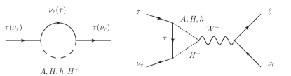
Figure 2: Dominant one-loop contributions to $\tau\to\ell\nu\nu$ in the lepton-specific 2HDM (adapted from Ref. Krawczyk and Temes (2005)).

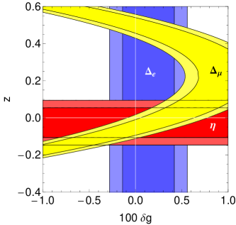
Figure 3: Allowed regions for $z$ and $\delta g$ from $\Delta_{\mu}$ (yellow), $\Delta_{e}$ (blue), and the Michel parameter $\eta$ (red); see text for definitions. Darker regions are at the $2\sigma$ level, lighter regions at $3\sigma$ one. Here we used for the experimental input the PDG values.

At tree level, only the charged scalar $H^{+}$ contributes to $\tau\to\ell\nu\nu$ in the lepton-specific 2HDM. (Note that the contributions in the type-X model are the same as in the type-II model as the lepton sector is identical.) Due to the small electron Yukawa couplings, the contributions to $\Delta_{e}^{\mathrm{tree}}$ are highly suppressed compared to $\Delta_{e}^{\mathrm{tree}}$, resulting in lepton flavour non-universality Hollik and Sack (1992); Krawczyk and Temes (2005); Aoki et al. (2009). However, one-loop corrections can be important as well (Fig. 2), and contribute (to a very good approximation) universally to $\Delta_{\ell}$ Hollik and Sack (1992); Krawczyk and Temes (2005) by modifying the $W\tau\nu$ couplings Abe et al. (2015)

$$g_{W\tau\nu}\to g_{W\tau\nu}(1+\delta g)\,.$$ (32)

For $m_{\mu}\ll m_{\tau}$ and $\delta g\ll 1$, we find (notation of Eq. (8))

$$\Delta_{e} \simeq 2\delta g\,,$$ (33)

$$\Delta_{\mu} \simeq 2\delta g+\frac{z^{2}}{4}-2z\frac{m_{\mu}}{m_{\tau}}\,,$$ (34)

with the charged-scalar coupling (assumed to be real)

$$z\equiv\frac{v^{2}}{m_{H^{+}}^{2}}\Gamma^{LR\,H^{+}}_{\nu_{\tau}\tau}\Gamma^{LR\,H^{+}\star}_{\nu_{\mu}\mu}\,.$$ (35)

Here we ignored flavour-changing interactions, which would not interfere with the SM and are tightly constrained from flavour-changing neutral current processes. In addition, the $H^{+}$ contribution to $\tau\to\mu\nu\nu$ leads to a non-zero Michel parameter $\eta=-2z/(4+z^{2})$ Abe et al. (2015), measured to be $\eta=0.013\pm 0.020$ Olive et al. (2014). The constraints (using the full expressions for $\Delta_{\ell}$ including lepton masses Abe et al. (2015)) are shown in Fig. 3 using PDG values. The SM value is recovered for $\delta g=z=0$.

In the SM-like limit $\sin(\beta-\alpha)=1$, and ignoring again flavour-violating couplings, we have Abe et al. (2015)

$$\delta g=\frac{\tan^{2}\beta}{32\pi^{2}}\left|\frac{m_{\tau}}{v}-\epsilon^{\ell}_{33}\right|^{2}\left[F\left(\frac{m_{A}^{2}}{m_{H^{+}}^{2}}\right)+F\left(\frac{m_{H}^{2}}{m_{H^{+}}^{2}}\right)\right],$$ (36)

with the loop function

$$F(x)\equiv\frac{1}{2}+\frac{1+x}{4(1-x)}\log x\,.$$ (37)

In particular, $F(x)\leq 0$ (equality for $x=1$), and so $\delta g\leq 0$. In the 2HDM-X, $z$ is positive and $\delta g$ negative, making it hard to reconcile both $\Delta_{e}$ and $\Delta_{\mu}$ unless rather high values of $z\simeq 0.5$ are chosen, which are then in disagreement with the Michel parameter $\eta$ Abe et al. (2015).

In our model, we can however flip the sign of the $\tau$ couplings for $\epsilon^{\ell}_{33}>m_{\tau}/v$, which allows for a negative $z$ ($\delta g$ remains negative) as we will see in the phenomenology section. Small values $z\simeq-0.1$ are then sufficient to satisfy the $\Delta_{\ell}$ constraints as well as $\eta$. Using HFAG values for the $\tau$ decay opens up parameter space at the $2\sigma$ level, see Fig. 7.

III.3 Magnetic moment $a_{\mu}$ and $\tau\to\mu\gamma$

The radiative decay $\tau\to\mu\gamma$ is closely related to the anomalous magnetic moment of the muon. Both observables are induced by penguin diagrams with internal neutral or charged Higgs bosons. The results can be encoded in the effective Hamiltonian

$${\cal{H}}_{\rm eff}=c^{\ell_{f}\ell_{i}}_{R}\,O^{\ell_{f}\ell_{i}}_{R}+c^{\ell_{f}\ell_{i}}_{L}\,O^{\ell_{f}\ell_{i}}_{L}\,,$$ (38)

where $c^{\ell_{f}\ell_{i}}_{R}$ and $c^{\ell_{f}\ell_{i}}_{L}$ are the Wilson coefficients of the magnetic dipole operators

$$O^{\ell_{f}\ell_{i}}_{R(L)}=m_{\ell_{i}}\bar{\ell}_{f}\sigma_{\mu\nu}P_{R(L)}\ell_{i}F^{\mu\nu}\,.$$ (39)

With these conventions, the branching ratio for the radiative lepton decays $\ell_{i}\to\ell_{f}\gamma$ reads

$${\rm BR}(\ell_{i}\to\ell_{f}\gamma)\,=\,\dfrac{m_{\ell_{i}}^{5}}{4\pi\,\Gamma_{\ell_{i}}}\left(|c^{\ell_{f}\ell_{i}}_{R}|^{2}+|c^{\ell_{f}\ell_{i}}_{L}|^{2}\right),$$ (40)

and the contribution to the anomalous magnetic moment of the muon is given by

$$\delta a_{\mu}=\,-\dfrac{4m^{2}_{\mu}}{e}\,\Re\left[{c^{\ell_{2}\ell_{2}}_{R}}\right].$$ (41)

The one-loop (and dominant two-loop) Wilson coefficients $c_{L,R}$ are given in App. A.

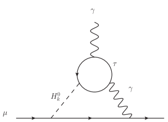
Figure 4: Dominating Barr–Zee diagram of a light scalar $H^{0}_{k}=A,H$ to $(g-2)_{\mu}$.

It is well known that two-loop Barr–Zee-type diagrams Barr and Zee (1990) can dominate in some regions of parameter space due to enhancement factors $m_{f}^{2}/m_{\mu}^{2}$ from fermions $f$ in the loop, which can overcome the additional loop suppression $\alpha_{\mathrm{EM}}/\pi$. For the 2HDM-X, there is an additional $\tan\beta$ enhancement for $A$, $H$, and enhanced two-loop contributions come from the $\tau$ in the loop (Fig. 4). However, there are other important diagrams which could give relevant contributions Chang et al. (1993); Hisano et al. (2006); Jung and Pich (2014); Abe et al. (2014); Ilisie (2015). While all diagrams involving $Z$ or $W$ bosons coupling to the external lepton line are highly suppressed, the diagrams with a closed charged Higgs loop or a $W$ loop connected to the external lepton line by a photon could be numerically relevant (replacing the $\tau$ in Fig. 4 by a $H^{+}$ or a $W$). Without explicit calculation (the detailed results are given in App. A) one can already deduce the scaling of the relevant diagrams:

$\tau$:

  $\Gamma^{H_{k}^{0}LR}_{fi}\frac{m_{\tau}}{v}\tan^{2}\beta$  (for $H_{k}^{0}=A,H$),

$H^{+}$:

  $\Gamma^{H_{k}^{0}LR}_{fi}\lambda_{H^{+}H^{-}H}\tan\beta$  (for $H_{k}^{0}=H$),

$W$:

  $\Gamma^{H_{k}^{0}LR}_{fi}\cos(\alpha-\beta)\frac{m_{W}}{v}\tan\beta$  (for $H_{k}^{0}=H$).

Here we included only the $A$ and $H$ contributions, as the coupling of $h$ to leptons is suppressed. The couplings of $A$ to $WW$ and $H^{+}H^{-}$ vanish due to CP conservation.

It was pointed out in Ref. Ilisie (2015) that the Higgs self-coupling $\lambda_{H^{+}H^{-}H}$ contribution can be very important. For this result, Ref. Ilisie (2015) allowed $\lambda_{H^{+}H^{-}H}$ to vary between $-5$ and $5$. However, $\lambda_{H^{+}H^{-}H}$ is not a fundamental parameter. It depends on the Higgs self-coupling in the scalar potential, but their contribution is suppressed by $1/\tan\beta$ and therefore negligible (see Eq. (62)). The diagram involving a $W$ loop can be important for moderate values of $\tan\beta$ Chang et al. (1993), but vanishes in the SM-like limit $\sin(\beta-\alpha)=1$. We will see later, $\sin(\beta-\alpha)\neq 1$ is required for explaining $h\to\mu\tau$. Nonetheless, working at large $\tan\beta$, as preferred by $\tau$ decays, we checked that also the contribution of the $W$ diagram is numerically small and does not change our conclusion for $(g-2)_{\mu}$.

III.4 Flavour changing top decays $t\to Hc$

Since we allow for a non-zero $\epsilon^{u}_{32}$ coupling, the top quark can decay into $H^{0}_{k}+c$ if the scalar $H^{0}_{k}=h,H,A$ is sufficiently light. For the branching ratio we find

$${\rm BR}(t\to H^{0}_{k}c)=\dfrac{m_{t}}{32\pi\Gamma_{t}}\left|\Gamma^{H^{0}_{k}LR}_{tc}\right|^{2}\left(1-\dfrac{m_{H^{0}_{k}}^{2}}{m_{t}^{2}}\right),$$ (42)

with the top decay width $\Gamma_{t}=(2\pm 0.5)\,$GeV.

III.5 Leptonic Higgs decays

The decay $h\to\tau\tau$ has been observed by CMS Chatrchyan et al. (2014) and ATLAS Aad et al. (2015) with $\mu$-parameters (relative strength compared to the SM prediction) $0.78\pm 0.27$ and $1.43^{+0.43}_{-0.37}$, respectively. A naive combination (also averaging the ATLAS result to $1.43\pm 0.40$) gives

$$\mu_{\tau\tau}=0.98\pm 0.22\,.$$ (43)

In our model, the decay rate for $h\to\tau\tau$ relative to the SM prediction takes the form

$$\mu_{\tau\tau}\simeq\frac{{\rm BR}\left(h\to\tau\tau\right)}{{\rm BR}\left(h\to\tau\tau\right)_{\text{SM}}}=\sin^{2}\alpha\tan^{2}\beta\left|1-\frac{\epsilon^{\ell}_{33}}{m_{\tau}/v}\right|^{2},$$ (44)

in the large $\tan\beta$ limit, assuming a SM-like production rate (in the SM-like limit $\sin(\beta-\alpha)\to 1$ we get back $\mu_{\tau\tau}\to 1$). The entry $\epsilon^{\ell}_{32}$ allows for the flavour-violating decay $h\to\mu\tau$ if $\cos(\alpha-\beta)\neq 0$:

$${\rm BR} \left(h\to\mu\tau\right)\simeq\dfrac{m_{h}}{8\pi\Gamma_{h}}\left|{\Gamma^{h\,LR}_{\tau\mu}}\right|^{2},$$ (45)

where $\Gamma_{h}\simeq 4.1\,$MeV is the decay width in the SM for the $125\,$GeV Brout–Englert–Higgs boson.

III.6 Other Higgs decays

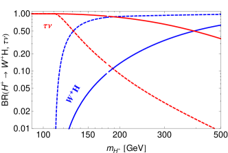
Figure 5: Branching ratios $H^{+}\to W^{+}H$ (blue) and $H^{+}\to\tau\nu$ (red) for $m_{H}=30\,\mathrm{GeV}$. Solid (dashed) lines are for $\tan\beta=80$ $(10)$.

With a light $H$, new decay modes open up, such as $h\to HH$, $A\to ZH$, and $H^{+}\to W^{+}H$ Gunion et al. (2000), followed by $H\to\tau\tau$ in the large $\tan\beta$ limit. (In complete analogy to the case where $A$ is light, see e.g. Cao et al. (2009).) The decay rates are given by

$$\Gamma(H^{+}\to W^{+}H) \simeq\frac{\alpha_{\mathrm{EM}}}{48s_{W}^{2}}\frac{m_{H^{+}}^{3}}{m_{W}^{2}}\left(1-\frac{m_{W}^{2}}{m_{H^{+}}^{2}}\right)^{3},$$ (46)

$$\Gamma(A\to ZH) \simeq\frac{\alpha_{\mathrm{EM}}}{48s_{W}^{2}c_{W}^{2}}\frac{m_{A}^{3}}{m_{Z}^{2}}\left(1-\frac{m_{Z}^{2}}{m_{A}^{2}}\right)^{3},$$ (47)

in the SM-like limit $\sin(\beta-\alpha)\simeq 1$ and for $m_{H}\ll m_{W}$. ($h\to HH$ depends on additional parameters and will not be discussed here.) If $\tan\beta$ is not too large, these channels can contribute significantly to the total decay rates of $H^{+}$ and $A$ (see Fig. 5), which weakens the direct search bounds on these particles (these bounds often assume 100% decays into tau leptons for the 2HDM-X).

III.7 Z boson decays

In the large $\tan\beta$ limit one expects a sizable modification of $Z\to\tau\tau$ at the loop level. Following Ref. Abe et al. (2015) we define the ratio of decays

$$R_{\tau/e}\equiv\frac{\Gamma(Z\to\tau\tau)}{\Gamma(Z\to ee)},$$ (48)

with the experimental value $R^{\text{exp}}_{\tau/e}=1.0019\pm 0.0032$ Olive et al. (2014). The deviation from the SM due to 2HDM vertex corrections is given by

$$\begin{split}\Delta R_{\tau/e}&\equiv R_{\tau/e}-R_{\tau/e}^{\text{SM}}\\ &\simeq\frac{g_{Z}^{2}m_{Z}/6\pi}{\Gamma(Z\to\ell\ell)_{\text{SM}}}\left[v_{\tau}\Re\Delta v_{\tau}^{\text{loop}}+a_{\tau}\Re\Delta a_{\tau}^{\text{loop}}\right],\end{split}$$ (49)

with $v_{\tau}=\frac{1}{2}T_{3}-s_{W}^{2}Q_{\tau}=s_{W}^{2}-1/4$ and $a_{\tau}=\frac{1}{2}T_{3}=-1/4$ being the tree level $Z\tau\tau$ couplings and

$$\begin{split}\Delta v_{\tau}^{\text{loop}}&\simeq\frac{\tan^{2}\beta}{32\pi^{2}}\left(\frac{m_{\tau}}{v}-\epsilon^{\ell}_{33}\right)^{2}\left[v_{\tau}(F_{1}(m_{H})+F_{1}(m_{A}))\right.\\ &\left.\quad-2a_{\tau}F_{1}(m_{H^{+}})+(v_{\tau}+a_{\tau})F_{2}(m_{H^{+}},m_{H^{+}})\right],\\ \Delta a_{\tau}^{\text{loop}}&\simeq-\frac{\tan^{2}\beta}{32\pi^{2}}\left(\frac{m_{\tau}}{v}-\epsilon^{\ell}_{33}\right)^{2}\left[a_{\tau}(F_{1}(m_{H})+F_{1}(m_{A}))\right.\\ &\left.\quad-2a_{\tau}F_{1}(m_{H^{+}})+(v_{\tau}+a_{\tau})F_{2}(m_{H^{+}},m_{H^{+}})\right.\\ &\left.\quad-4a_{\tau}F_{2}(m_{H},m_{A})\right],\end{split}$$ (50)

in the SM-like limit $\sin(\beta-\alpha)=1$. The loop functions $F_{j}$ can be found in Ref. Abe et al. (2015). For the region of interest the limits from $Z$ decays are of similar order as those from $\tau\to\ell\nu\nu$.

For $\epsilon_{32}^{\ell}\neq 0$, one also induces $Z\to\mu\tau$ via a similar one-loop diagram Goto et al. (2015). For the mass ranges of interest in this work the branching ratio is approximately

$${\rm BR}(Z\to\mu\tau)\simeq 5\times 10^{-5}\left(\frac{\epsilon_{32}^{\ell}}{10^{-2}}\right)^{2}\left(\frac{\tan\beta}{100}\right)^{4}.$$ (51)

The best upper limit of $1.2\times 10^{-5}$ at $95\%$ C.L. Olive et al. (2014) still comes from LEP, but LHC searches should be able to improve this by a factor of few with current data Davidson et al. (2012) and even more with the upcoming run.

IV Phenomenological Analysis

Using the formulae collected in the last section, we now study the phenomenology of our 2HDM and show that it can indeed resolve the anomalies outlined in the introduction.

IV.1 ${\cal R}(D)$ and ${\cal R}(D^{*})$

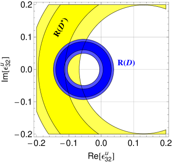
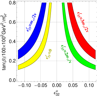
Figure 6: Left: Allowed regions in the $\epsilon^{u}_{32}$-plane from ${\cal R}(D)$ (blue) and ${\cal R}(D^{*})$ (yellow) for $\tan\beta=50$, $m_{H^{+}}=200$ GeV, and $\epsilon^{\ell}_{33}=0$. The scaling of the allowed region for $\epsilon^{u}_{32}$ with $\tan\beta$ and $m_{H^{+}}$ is the same as for $\epsilon^{u}_{31}$. $\epsilon^{u}$ is given at the matching scale $m_{H^{+}}$. Right: Allowed regions in the $\epsilon^{u}_{32}$–$\dfrac{\tan\beta}{100}\dfrac{(100\,{\rm GeV})^{2}}{m_{H^{+}}^{2}}$ plane for $\epsilon^{\ell}_{33}=0$ (yellow), $\dfrac{m_{\tau}}{2v}$ (blue), $\dfrac{3m_{\tau}}{2v}$ (red) and $\dfrac{2m_{\tau}}{v}$ (green).

Let us first consider ${\cal R}(D)$ and ${\cal R}(D^{*})$. From the left plot of Fig. 6 we see that ${\cal R}(D)$ and ${\cal R}(D^{*})$ can be explained simultaneously for negative values of $\epsilon^{u}_{32}$ with small or vanishing imaginary part. The right plot in Fig. 6 shows the dependence of $\epsilon^{u}_{32}$ on $\dfrac{\tan\beta}{100}\dfrac{(100\,{\rm GeV})^{2}}{m_{H^{+}}^{2}}$ requiring that ${\cal R}(D)$ and ${\cal R}(D^{*})$ are explained. Note that sizable values of $\epsilon^{u}_{32}$ are required, i.e. of the order of $10^{-1}$. This is important for $t\to Hc$ to be considered later.

IV.2 $\tau\to\ell\nu\nu$

The tree-level charged Higgs contribution interferes destructively with the SM for $\epsilon_{33}^{\ell}=0$. However, for $\epsilon_{33}^{\ell}>m_{\tau}/v$ the interference is constructive, allowing for an explanation of the PDG data, which is in more than a $2\sigma$ tension with the SM. The 1-loop contributions interfere again destructively (independently of $\epsilon_{33}$) and are important for non-degenerate $A$ and $H$ masses. Nonetheless, even if $m_{H}=30\,$GeV and $m_{A}=200\,$GeV, the values $m_{H^{+}}=200\,$ GeV, $\epsilon_{33}^{\ell}=2m_{\tau}/v$ and $\tan\beta>60$ are consistent with data (see Fig. 7). Furthermore, as one can also see from Fig. 7, for $\epsilon^{u}_{32}\approx 0.1$ also ${\cal R}(D)$ and ${\cal R}(D^{*})$ can be brought into agreement with the measurements. Therefore, the possibility to flip the sign of the $H,A$ coupling to taus allows us to have smaller values $\tan\beta$ than in the 2HDM-X.

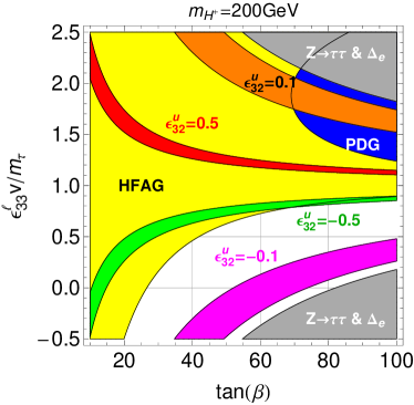
Figure 7: Allowed regions in the $\tan\beta$–$v/m_{\tau}\epsilon^{\ell}_{33}$ plane from ${\cal R}(D^{(*)})$ and $\tau\to\mu\nu\nu$ at the $2\,\sigma$ level. The yellow region is allowed by $\tau\to\mu\nu\nu$ using the HFAG result for $m_{H}=30\,$GeV and $m_{A}=200\,$GeV, while the (darker) blue one is the allowed region using the PDG result. The red, orange, green and magenta bands correspond to the allowed regions by ${\cal R}(D^{(*)})$ for different values of $\epsilon^{u}_{32}$. The gray region is excluded by $Z\to\tau\tau$ and $\tau\to e\nu\nu$. For $m_{H}\approx m_{A}$ the allowed regions from $\tau\to\mu\nu\nu$ would be slightly larger.

IV.3 Anomalous magnetic moment of the muon

In the anomalous magnetic moment of the muon, the one-loop and the two-loop Barr–Zee contribution have opposite sign for $\epsilon^{\ell}_{33}=0$ (neglecting flavour violating couplings). However, for $\epsilon^{\ell}_{33}>m_{\tau}/v$ the interference is constructive, allowing for an explanation with smaller values of $\tan\beta$ and/or heavier Higgses. Note that for $\epsilon^{\ell}_{33}>m_{\tau}/v$ the $H$ contribution has the same sign as the SM contribution while the $A$ one has opposite sign, so in our scenario it is a light $H$ that can solve the $\Delta a_{\mu}$ anomaly, as opposed to a light $A$ in the standard 2HDM-X. We show explicitly in the left plot of Fig. 8 that $m_{H}$ must be smaller than $m_{A}$ for $\epsilon^{\ell}_{33}>m_{\tau}/v$. As seen above, $\epsilon^{\ell}_{33}>m_{\tau}/v$ is preferred by $\tau\to\mu\nu\nu$.

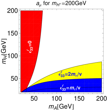
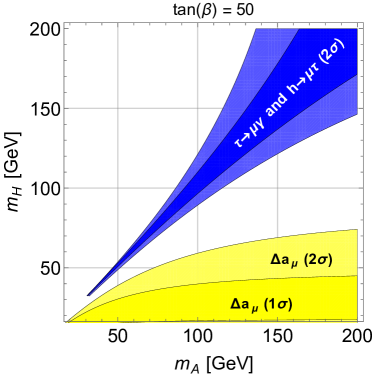
Figure 8: Left: Allowed regions in the $m_{A}$–$m_{H}$ plane from the anomalous magnetic moment of the muon at the $2\,\sigma$ level for $\tan\beta=70$, $m_{H^{+}}=200\,$GeV, $\cos(\alpha-\beta)=0$ and different values of $\epsilon^{\ell}_{33}$. Right: Allowed regions in the $m_{A}$-$m_{H}$ plane from $(g-2)_{\mu}$, $\tau\to\mu\gamma$ and $h\to\mu\tau$ for $\tan(\beta)=30$ and $\epsilon^{\ell}_{33}=2m_{\tau}/v$. For $h\to\tau\mu$ blue corresponds to $\cos(\alpha-\beta)=0.1$ and light blue to $\cos(\alpha-\beta)=0.2$. The allowed region for $\Delta a_{\mu}$ is maximal in the sense that we allowed for the three possibilities $\epsilon^{\ell}_{32}\neq 0$, $\epsilon^{\ell}_{32}=\epsilon^{\ell}_{23}\neq 0$ and $\epsilon^{\ell}_{32}=-\epsilon^{\ell}_{23}\neq 0$ as the latter ones can give $m_{\tau}/m_{\mu}$ enhanced one-loop contributions. However, the effects turns out to be small, as $\epsilon^{\ell}_{32,32}$ is stringently constrained from $\tau\to\mu\gamma$. In addition, we checked that the effect of $\lambda_{H}$ is very small.

IV.4 $h\to\mu\tau$ and $\tau\to\mu\gamma$

Until now, we worked in the large $\tan\beta$ limit with $\alpha=0$. However, the decay $h\to\mu\tau$ can only appear for non-zero values of $\cos(\alpha-\beta)$. In this case additional Barr–Zee diagrams with gauge bosons or top quarks can contribute to $\tau\to\mu\gamma$ (see App. A). Therefore, the analysis is more involved than the one for the anomalous magnetic moment of the muon. However, as we have shown in the case of $(g-2)_{\mu}$ (where the contributions are directly related to $\tau\to\mu\gamma$), $\cos(\alpha-\beta)\neq 0$ has actually only a small effect on the result.

To explain the CMS excess in $h\to\mu\tau$ (Eq. (10)), one needs a coupling strength of approximately

$$\sin\alpha\tan\beta|\epsilon^{\ell}_{32}|\simeq 3.7\times 10^{-3}\,.$$ (52)

Non-zero values of $\epsilon^{\ell}_{32}$ then give rise to $\tau\to\mu\gamma$. The experimental upper limit for $\tau\to\mu\gamma$ is given by Aubert et al. (2010); Hayasaka et al. (2008)

$${\rm BR}\left(\tau\to\mu\gamma\right)\leq 4.4\times 10^{-8}\,,$$ (53)

at $90\%$ C.L.. It is interesting to see if one can explain $h\to\mu\tau$ and $(g-2)_{\mu}$ simultaneously without violating bounds from $\tau\to\mu\gamma$. As the loop contributions to $\tau\to\mu\gamma$ are governed by the same Wilson coefficients as $(g-2)_{\mu}$ (see Sec. III.2), this turns out to be challenging. In the right plot of Fig. 8 we show the allowed regions in the $m_{A}$–$m_{H}$ plane for $\tau\to\mu\gamma$, $h\to\mu\tau$ and $(g-2)_{\mu}$. As one can see, there is no overlap among all regions. There is an $m_{\tau}/m_{\mu}$ enhanced contribution to $(g-2)_{\mu}$ in the case $\epsilon_{23}^{\ell}\neq 0$ and $\epsilon_{32}^{\ell}\neq 0$. Even though we restricted ourselves in Eq. (27) to vanishing values of $\epsilon_{23}^{\ell}\neq 0$, we checked that also for $\epsilon_{32}^{\ell}=\epsilon_{23}^{\ell}$ the effect in $(g-2)_{\mu}$ is small, taking into account the upper limit on $\epsilon_{32}^{\ell}=\epsilon_{23}^{\ell}$ from $\tau\to\mu\gamma$ while aiming at an explanation of $h\to\mu\tau$.

In principle, one might increase the coupling strength $\Gamma^{H,A,H^{+}}_{\mu\mu}$ with the help of $\epsilon_{22}^{\ell}$. This would soften the tight relationship

$$c_{R}^{\mu\tau}/c_{R}^{\mu\mu}\simeq\Gamma^{H^{0}_{k}}_{\mu\tau}/\Gamma^{H^{0}_{k}}_{\mu\mu}\simeq\epsilon^{\ell}_{32}v/m_{\mu}$$ (54)

originating from the dominant Barr–Zee diagram with a $\tau$ loop which causes the incompatibility of $a_{\mu}$ and $\tau\to\mu\gamma$ (Fig. 4). However, a large shift in $\Gamma^{H,A,H^{+}}_{\mu\mu}$ from $\epsilon^{\ell}_{22}\ll m_{\mu}/v$ would mean fine tuning and also strongly affect $\tau\to\mu\nu\nu$. Therefore, we conclude that explaining $a_{\mu}$ and $h\to\mu\tau$ simultaneously is not impossible, but rather difficult and would involve fine tuning.

IV.5 $t\to Hc$

For light values of $m_{H}$, as preferred by the anomalous magnetic moment of the muon, and non-zero values of $\epsilon^{u}_{32}$ as required by an explanation of ${\cal R}(D^{(*)})$, the flavour changing top decay $t\to Hc$ can have sizable branching ratios. In fact, as shown in Fig. 9 the branching ratio can be easily of the order of $10^{-2}$.

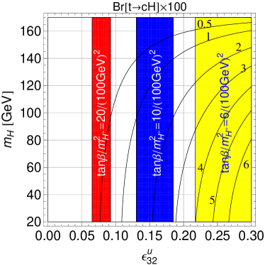
Figure 9: The contour lines denote ${\rm BR}(t\to Hc)\times 100$ as a function of $\epsilon^{u}_{32}$ and $m_{H}$. The coloured regions are allowed by ${\cal R}(D)$ and ${\cal R}(D^{*})$ for different values of $\tan\beta/m_{H^{+}}^{2}$.

V Conclusions

In this article we addressed the measured anomalies in ${\cal R}(D^{(*)})$ ($3.8\sigma$), $a_{\mu}$ ($\sim 3\sigma$), $\tau\to\mu\nu\nu$ ($2.4\sigma$), and $h\to\mu\tau$ ($2.4\sigma$) within a simple two-Higgs-doublet model. The Yukawa structure of our model is close to the lepton-specific 2HDM (type X), but with some additional Yukawa couplings involving third-generation fermions that give rise to the $b$–$c$ (necessary for ${\cal R}(D^{(*)})$) and $\mu$–$\tau$ transitions (relevant for $h\to\mu\tau$) as well as corrections to $\tau\tau$ couplings (important for $\tau\to\mu\nu\nu$).

Let us summarize the logic of the article.

• $\tau\to\mu\nu\nu$ prefers $\epsilon^{\ell}_{33}\geq m_{\tau}/v$. If one wants to account for the PDG average, also $\tan\beta>50$ is desirable.

• $a_{\mu}$ favours small values of $m_{H}$ for $\epsilon^{\ell}_{33}\geq m_{\tau}/v$ as in this case the Barr–Zee contribution with a $\tau$ loop has the correct sign and the diagram involving a Higgs self-coupling can be relevant.

• ${\cal R}(D)$ and ${\cal R}(D^{*})$ point towards quite large negative values of $\epsilon^{u}_{32}$ (of order $-0.1$).

• In case of a light $H$ (as preferred by $a_{\mu}$), sizable decay rates for $t\to Hc$ are possible if ${\cal R}(D)$ and ${\cal R}(D^{*})$ are explained via $\epsilon^{u}_{32}$. This decay could be observed at the LHC in the process $pp\to\bar{t}t$, $t\to Hc$, $H\to\tau\tau$.

• $h\to\mu\tau$ can be explained using $\epsilon^{\ell}_{32}$. In this case $\alpha\neq 0$ and constraints from $\tau\to\mu\gamma$ arise. As the Barr–Zee contributions in $\tau\to\mu\gamma$ are directly correlated to the ones in $a_{\mu}$, a simultaneous explanation is difficult.

• If one attempts to explain $h\to\mu\tau$ (disregarding $a_{\mu}$), the exotic process $pp\to\bar{t}t$, $t\to Hc$, $H\to\mu\tau$ can occur at the LHC.

Therefore, the future prospects are very promising: the decay $h\to\mu\tau$ implies rates for $\tau\to\mu\gamma$ in reach of future experiments. More data on tau leptons is necessary to test our model, in particular $\tau\to\ell\nu\nu$, $\tau\to\mu\gamma$, and $h\to\tau\tau$. Furthermore, the light $H$ and the flavour-changing couplings required for ${\cal R}(D^{(*)})$ lead to the decay $t\to Hc$, followed by $H\to\tau\tau$ (or even $H\to\mu\tau$), which can be searched for at the LHC. While we did not attempt to find a symmetry realisation of the pattern assumed for the $\epsilon^{f}_{ij}$ structures, it would be very interesting to find appropriate flavour symmetries to generate them dynamically, as the model works very well phenomenologically. An additional venue of interest would be the inclusion of dark matter in order to explain the galactic centre gamma-ray excess Hektor et al. (2015).

Appendix A Wilson coefficients for $a_{\mu}$ and $\ell_{i}\to\ell_{f}\gamma$

The effective Hamiltonian relevant for $\ell_{i}\to\ell_{f}\gamma$ and $a_{\mu}$ is given in Eq. (38) with operators from Eq. (39). The Hermiticity of the Hamiltonian allows us to deduce $c_{L}$ from $c_{R}$ in complete generality via

$$c^{\ell_{f}\ell_{i}}_{L}=\frac{m_{\ell_{f}}}{m_{\ell_{i}}}c^{\ell_{i}\ell_{f}*}_{R}\,,$$ (55)

so we will only show $c_{R}$ in the following. The final $c_{L,R}$ of course requires a sum over all the individual $c_{L,R}$ we present here.

At one loop the neutral Higgs ($H_{k}^{0}=H,h,A$) penguin contribution to $c^{\ell_{f}\ell_{i}}_{R}$ is given by

$$\begin{split}{c^{\ell_{f}\ell_{i}}_{R\,H^{0}}}&=\sum\limits_{k,j=1}^{3}\dfrac{-e}{192\pi^{2}m^{2}_{H^{0}_{k}}}\,\Bigg{[}\Gamma^{H_{k}^{0}\,LR}_{\ell_{f}\ell_{j}}\Gamma^{H_{k}^{0}\,LR\star}_{\ell_{i}\ell_{j}}\\ &\quad+\dfrac{m_{\ell_{f}}}{m_{\ell_{i}}}\Gamma^{H_{k}^{0}\,LR\star}_{\ell_{j}\ell_{f}}\Gamma^{H_{k}^{0}\,LR}_{\ell_{j}\ell_{i}}\\ &\quad-\dfrac{m_{\ell_{j}}}{m_{\ell_{i}}}\Gamma^{H_{k}^{0}\,LR}_{\ell_{f}\ell_{j}}\Gamma^{H_{k}^{0}\,LR}_{\ell_{j}\ell_{i}}\left(9+6\ln\left(\dfrac{m^{2}_{\ell_{j}}}{m^{2}_{H^{0}_{k}}}\right)\right)\Bigg{]},\end{split}$$ (56)

and the charged Higgs penguin contribution takes the form

$${c^{\ell_{f}\ell_{i}}_{R\,H^{+}}} =\dfrac{e}{384\pi^{2}m^{2}_{H^{+}}}\frac{m_{\ell_{f}}}{m_{\ell_{i}}}\sum\limits_{j=1}^{3}\Gamma^{H^{+}\,LR}_{\nu_{j}\ell_{i}}\Gamma^{H^{+}\,LR\star}_{\nu_{j}\ell_{f}}\,.$$ (57)

It is well known that two-loop Barr–Zee-type diagrams Barr and Zee (1990) (see Fig. 10) can dominate in some regions of parameter space due to enhancement factors $m_{f}^{2}/m_{\mu}^{2}$ from fermions $f$ in the loop, which can overcome the additional loop suppression $\alpha_{\mathrm{EM}}/\pi$. For the 2HDM-X, there is an additional $\tan\beta$ enhancement for $A$, $H$, and enhanced $2$-loop contributions come from the $\tau$ in the loop. However, there are in addition other important diagrams Chang et al. (1993); Hisano et al. (2006); Jung and Pich (2014); Abe et al. (2014); Ilisie (2015) that could give relevant contributions to be summarized and converted to our conventions in the following.

(a)

(b)

(c)

(d)

(e)

(f)

Figure 10: Barr–Zee diagrams relevant for the Wilson coefficients $c_{L,R}^{\ell_{f}\ell_{i}}$.

A.1 Diagram (a)

The most relevant Barr–Zee diagram contains an additional charged fermion $f$ in the loop (Fig. 10a).

$$c_{R}^{\ell_{f}\ell_{i},(a)}=\frac{-e^{3}}{128\pi^{4}}\sum_{f_{j}}\frac{N_{f}^{c}Q^{2}_{f}}{m_{\ell_{i}}}\sum_{i=h,H,A}\Gamma_{\ell_{f}\ell_{i}}^{i}\Gamma_{f_{j}f_{j}}^{i}\frac{m^{f_{j}}}{m_{i}^{2}}g_{i}^{(a)}(r_{f_{j}}^{i}),$$ (58)

where $N_{f}^{c}$ and $Q_{f}$ are the number of colours and charge of fermion $f$, respectively, and $r_{f}^{i}\equiv m_{f}^{2}/m_{i}^{2}$. The loop function is given by

$$g_{i}^{(a)}(r)=\int_{0}^{1}\mathrm{d}x\,\frac{N_{i}(x)}{x(1-x)-r}\ln\left(\frac{x(1-x)}{r}\right),$$ (59)

where

$$N_{h}(x)=N_{H}(x)=2x(1-x)-1\,,\quad N_{A}(x)=-1\,.$$ (60)

A.2 Diagram (b)

The diagram from Fig. 10b contains a charged scalar in the loop and hence depends on the $H^{+}H^{-}H_{i}^{0}$ self-interactions. The relevant dimensionless trilinear Higgs couplings are given by

$$\begin{split}\lambda_{H^{+}H^{-}h}&=-\frac{1}{v^{2}}\left(m_{H}^{2}-m_{h}^{2}\right)\frac{\sin(2\alpha+2\beta)\sin(\alpha-\beta)}{\sin(4\beta)}\\ &\quad-\frac{1}{v^{2}}\left(m_{H^{+}}^{2}-\frac{m_{h}^{2}}{2}\right)\sin(\alpha-\beta)\\ &\quad+\Delta\lambda\tan(2\beta)\cos(\alpha+\beta)\,,\end{split}$$ (61)

$$\begin{split}\lambda_{H^{+}H^{-}H}&=+\frac{1}{v^{2}}\left(m_{H}^{2}-m_{h}^{2}\right)\frac{\sin(2\alpha+2\beta)\cos(\alpha-\beta)}{\sin(4\beta)}\\ &\quad+\frac{1}{v^{2}}\left(m_{H^{+}}^{2}-\frac{m_{H}^{2}}{2}\right)\cos(\alpha-\beta)\\ &\quad+\Delta\lambda\tan(2\beta)\sin(\alpha+\beta)\,,\end{split}$$ (62)

and $\lambda_{H^{+}H^{-}A}=0$. $\Delta\lambda\equiv\lambda_{2}-\lambda_{1}$ is a free parameter Skiba and Kalinowski (1993). While the last two terms in Eq. (62) vanish in the SM-like limit $\sin(\beta-\alpha)=1$, the first is still suppressed by $1/\tan\beta$ for large $\tan\beta$. The Wilson coefficient is then given by Ilisie (2015)

$$\begin{split}c_{R}^{\ell_{f}\ell_{i},(b)}&=\frac{e^{3}}{128\sqrt{2}\pi^{4}}\frac{v}{m_{\ell_{i}}}\\ &\quad\times\sum_{i=h,H,A}\frac{\Gamma_{\ell_{f}\ell_{i}}^{i}}{m_{i}^{2}}\zeta^{i}\lambda_{H^{+}H^{-}H_{i}^{0}}g_{i}^{(b)}\left(\frac{m_{H^{+}}^{2}}{m_{i}^{2}}\right),\end{split}$$ (63)

where $\zeta^{h}=-\zeta^{H}=-\zeta^{A}=1$ and the loop function is

$$g_{h,H,A}^{(b)}(r)=\int_{0}^{1}\mathrm{d}x\,\frac{x(1-x)}{x(1-x)-r}\ln\left(\frac{r}{x(1-x)}\right).$$ (64)

A.3 Diagram (c)

The contribution of the diagram in Fig. 10c with a $W$ in the loop is Ilisie (2015):

$$c_{R}^{\ell_{f}\ell_{i},(c)}=\frac{G_{F}e^{3}}{64\pi^{4}}\sum_{i=h,H}\frac{v}{m_{\ell_{i}}}\Gamma_{\ell_{f}\ell_{i}}^{i}\zeta^{i}\mathcal{R}_{i1}\,g_{i}^{(c)}\left(\frac{m_{W}^{2}}{m_{i}^{2}}\right),$$ (65)

where $\mathcal{R}_{h1}=\sin(\beta-\alpha)$, $\mathcal{R}_{H1}=-\cos(\beta-\alpha)$ and the loop function is

$$\begin{split}g_{h,H}^{(c)}(r)&=\frac{1}{2}\int_{0}^{1}\mathrm{d}x\,\left[\frac{x(1-x)-xr[3x(4x-1)+10]}{x(1-x)-r}\right.\\ &\qquad\left.\times\ln\left(\frac{r}{x(1-x)}\right)\right].\end{split}$$ (66)

A.4 Diagrams (d), (e), (f)

Finally, there are three types of Barr-Zee diagrams, where the virtual $H_{i}^{0}$ and $\gamma$ propagators are replaced by $H^{+}$ and $W$: Figs. 10d (where the fermion line is a $t$/$b$- or $b$/$t$-loop), 10e and 10f. Defining the loop function

$$G(r^{a},r^{b})=\frac{\ln\left(\frac{r^{a}x+r^{b}(1-x)}{x(1-x)}\right)}{x(1-x)-r^{a}x-r^{b}(1-x)}\,,$$ (67)

and the matrix

$$\mathcal{R}=\left(\begin{matrix}\sin(\beta-\alpha)&\cos(\beta-\alpha)&0\\ -\cos(\beta-\alpha)&\sin(\beta-\alpha)&0\\ 0&0&1\end{matrix}\right),$$ (68)

the diagrams in Fig. 10d, 10e and 10f are Ilisie (2015)

$$\begin{split}c_{R}^{\ell_{f}\ell_{i},(d)}&=\frac{-e^{3}}{1024\pi^{4}\sin^{2}\theta_{w}}\frac{N^{c}_{t}V_{tb}^{*}}{(m_{H^{+}}^{2}-m_{W}^{2})}\int_{0}^{1}\mathrm{d}x\,\left(Q_{t}x+Q_{b}(1-x)\right)\left[G\left(\frac{m_{t}^{2}}{m_{H^{+}}^{2}},\frac{m_{b}^{2}}{m_{H^{+}}^{2}}\right)-G\left(\frac{m_{t}^{2}}{m_{W}^{2}},\frac{m_{b}^{2}}{m_{W}^{2}}\right)\right]\\ &\quad\times\left[\left({\Gamma_{tb}^{H^{+},LR}}^{*}{\Gamma_{\nu_{f}\ell_{i}}^{H^{+}}}\right)\frac{m_{b}}{m_{\ell_{i}}}x(1-x)-\left({\Gamma_{tb}^{H^{+},RL}}^{*}{\Gamma_{\nu_{f}\ell_{i}}^{H^{+}}}\right)\frac{m_{t}}{m_{\ell_{i}}}x(1+x)\right],\end{split}$$ (69)

$$\begin{split}c_{R}^{\ell_{f}\ell_{i},(e)}&=\frac{G_{F}e^{3}}{64\pi^{4}\sqrt{2}}\frac{1}{8\sin^{2}\theta_{w}}\sum_{i}\frac{v}{m_{\ell_{i}}}{\Gamma_{\nu_{f}\ell_{i}}^{H^{+}}}(\mathcal{R}_{i1}(\mathcal{R}_{i2}-i\mathcal{R}_{i3}))^{*}\int_{0}^{1}\mathrm{d}x\,x^{2}\\ &\quad\times\left(\frac{(m_{H^{+}}^{2}+m_{W}^{2}-m_{i}^{2})(1-x)-4m_{W}^{2}}{m_{H^{+}}^{2}-m_{W}^{2}}\right)\left[G\left(\frac{m_{W}^{2}}{m_{H^{+}}^{2}},\frac{m_{i}^{2}}{m_{H^{+}}^{2}}\right)-G\left(1,\frac{m_{i}^{2}}{m_{W}^{2}}\right)\right],\end{split}$$ (70)

$$\begin{split}c_{R}^{\ell_{f}\ell_{i},(f)}&=\frac{G_{F}e^{3}}{64\pi^{4}\sqrt{2}}\frac{1}{4\sin^{2}\theta_{w}}\frac{v^{2}}{(m_{H^{+}}^{2}-m_{W}^{2})}\sum_{i}\frac{v}{m_{\ell_{i}}}{\Gamma_{\nu_{f}\ell_{i}}^{H^{+}}}(\mathcal{R}_{i2}-i\mathcal{R}_{i3})^{*}\zeta^{i}\lambda_{H^{+}H^{-}H^{0}_{i}}\\ &\quad\times\int_{0}^{1}\mathrm{d}x\,x^{2}(x-1)\left[G\left(1,\frac{m_{i}^{2}}{m_{H^{+}}^{2}}\right)-G\left(\frac{m_{H^{+}}^{2}}{m_{W}^{2}},\frac{m_{i}^{2}}{m_{W}^{2}}\right)\right].\end{split}$$ (71)

References

- Krawczyk and Pokorski (1988) P. Krawczyk and S. Pokorski, Phys.Rev.Lett. 60, 182 (1988).
- Bennett et al. (2006) G. Bennett et al. (Muon Collaboration), Phys.Rev. D73, 072003 (2006), eprint [arXiv:hep-ex/0602035].
- Olive et al. (2014) K. Olive et al. (Particle Data Group), Chin.Phys. C38, 090001 (2014).
- Aoyama et al. (2012) T. Aoyama, M. Hayakawa, T. Kinoshita, and M. Nio, Phys.Rev.Lett. 109, 111808 (2012), eprint [arXiv:1205.5370 [hep-ph]].
- Czarnecki et al. (1995) A. Czarnecki, B. Krause, and W. J. Marciano, Phys.Rev. D52, 2619 (1995), eprint [arXiv:hep-ph/9506256].
- Czarnecki et al. (1996) A. Czarnecki, B. Krause, and W. J. Marciano, Phys.Rev.Lett. 76, 3267 (1996), eprint [arXiv:hep-ph/9512369].
- Gnendiger et al. (2013) C. Gnendiger, D. Stöckinger, and H. Stöckinger-Kim, Phys.Rev. D88, 053005 (2013), eprint [arXiv:1306.5546 [hep-ph]].
- Davier et al. (2011) M. Davier, A. Hoecker, B. Malaescu, and Z. Zhang, Eur.Phys.J. C71, 1515 (2011), eprint [arXiv:1010.4180 [hep-ph]].
- Hagiwara et al. (2011) K. Hagiwara, R. Liao, A. D. Martin, D. Nomura, and T. Teubner, J.Phys. G38, 085003 (2011), eprint [arXiv:1105.3149 [hep-ph]].
- Kurz et al. (2014) A. Kurz, T. Liu, P. Marquard, and M. Steinhauser, Phys.Lett. B734, 144 (2014), eprint [arXiv:1403.6400 [hep-ph]].
- Jegerlehner and Nyffeler (2009) F. Jegerlehner and A. Nyffeler, Phys.Rept. 477, 1 (2009), eprint [arXiv:0902.3360 [hep-ph]].
- Colangelo et al. (2014a) G. Colangelo, M. Hoferichter, A. Nyffeler, M. Passera, and P. Stoffer, Phys.Lett. B735, 90 (2014a), eprint [arXiv:1403.7512 [hep-ph]].
- Colangelo et al. (2014b) G. Colangelo, M. Hoferichter, M. Procura, and P. Stoffer, JHEP 1409, 091 (2014b), eprint [arXiv:1402.7081 [hep-ph]].
- Colangelo et al. (2014c) G. Colangelo, M. Hoferichter, B. Kubis, M. Procura, and P. Stoffer, Phys. Lett. B738, 6 (2014c), eprint [arXiv:1408.2517 [hep-ph]].
- Colangelo et al. (2015) G. Colangelo, M. Hoferichter, M. Procura, and P. Stoffer (2015), eprint arXiv:1506.01386 [hep-ph].
- Hayakawa et al. (2006) M. Hayakawa, T. Blum, T. Izubuchi, and N. Yamada, PoS LAT2005, 353 (2006), eprint [arXiv:hep-lat/0509016].
- Blum et al. (2012) T. Blum, M. Hayakawa, and T. Izubuchi, PoS LATTICE2012, 022 (2012), eprint [arXiv:1301.2607 [hep-lat]].
- Blum et al. (2015) T. Blum, S. Chowdhury, M. Hayakawa, and T. Izubuchi, Phys.Rev.Lett. 114, 012001 (2015), eprint [arXiv:1407.2923 [hep-lat]].
- Green et al. (2015) J. Green, O. Gryniuk, G. von Hippel, H. B. Meyer, and V. Pascalutsa (2015), eprint arXiv:1507.01577 [hep-lat].
- Stöckinger (2007) D. Stöckinger, J. Phys. G34, R45 (2007), eprint hep-ph/0609168.
- Langacker (2009) P. Langacker, Rev. Mod. Phys. 81, 1199 (2009), eprint 0801.1345.
- Baek et al. (2001) S. Baek, N. G. Deshpande, X. G. He, and P. Ko, Phys. Rev. D64, 055006 (2001), eprint hep-ph/0104141.
- Ma et al. (2002) E. Ma, D. P. Roy, and S. Roy, Phys. Lett. B525, 101 (2002), eprint hep-ph/0110146.
- Gninenko and Krasnikov (2001) S. N. Gninenko and N. V. Krasnikov, Phys. Lett. B513, 119 (2001), eprint hep-ph/0102222.
- Pospelov (2009) M. Pospelov, Phys. Rev. D80, 095002 (2009), eprint 0811.1030.
- Heeck and Rodejohann (2011) J. Heeck and W. Rodejohann, Phys. Rev. D84, 075007 (2011), eprint 1107.5238.
- Harigaya et al. (2014) K. Harigaya, T. Igari, M. M. Nojiri, M. Takeuchi, and K. Tobe, JHEP 03, 105 (2014), eprint 1311.0870.
- Altmannshofer et al. (2014) W. Altmannshofer, S. Gori, M. Pospelov, and I. Yavin, Phys.Rev.Lett. 113, 091801 (2014), eprint 1406.2332.
- Chakraverty et al. (2001) D. Chakraverty, D. Choudhury, and A. Datta, Phys.Lett. B506, 103 (2001), eprint hep-ph/0102180.
- Cheung (2001) K.-m. Cheung, Phys. Rev. D64, 033001 (2001), eprint hep-ph/0102238.
- Freitas et al. (2014) A. Freitas, J. Lykken, S. Kell, and S. Westhoff, JHEP 05, 145 (2014), [Erratum: JHEP09,155(2014)], eprint 1402.7065.
- Iltan and Sundu (2003) E. O. Iltan and H. Sundu, Acta Phys. Slov. 53, 17 (2003), eprint hep-ph/0103105.
- Omura et al. (2015) Y. Omura, E. Senaha, and K. Tobe, JHEP 1505, 028 (2015), eprint 1502.07824.
- Broggio et al. (2014) A. Broggio, E. J. Chun, M. Passera, K. M. Patel, and S. K. Vempati, JHEP 1411, 058 (2014), eprint 1409.3199.
- Wang and Han (2015) L. Wang and X.-F. Han, JHEP 1505, 039 (2015), eprint 1412.4874.
- Abe et al. (2015) T. Abe, R. Sato, and K. Yagyu, JHEP 07, 064 (2015), eprint 1504.07059.
- Lees et al. (2012a) J. Lees et al. (BABAR Collaboration), Phys.Rev.Lett. 109, 101802 (2012a), eprint 1205.5442.
- Chur (2015) T. Chur (Belle), Talk at the FPCP conference 2015, https://agenda.hepl.phys.nagoya-u.ac.jp/indico/getFile.py/access?contribId=22&sessionId=4&resId=0&materialId=slides&confId=170 (2015).
- Huschle et al. (2015) M. Huschle et al. (Belle) (2015), eprint 1507.03233.
- Aaij et al. (2015) R. Aaij et al. (LHCb) (2015), eprint 1506.08614.
- Rotondo (2015) M. Rotondo, Talk of Zoltan Ligeti at the FPCP conference 2015, https://agenda.hepl.phys.nagoya-u.ac.jp/indico/getFile.py/access?contribId=9&sessionId=19&resId=0&materialId=slides&confId=170 (2015).
- Kamenik and Mescia (2008) J. F. Kamenik and F. Mescia, Phys.Rev. D78, 014003 (2008), eprint 0802.3790.
- Fajfer et al. (2012a) S. Fajfer, J. F. Kamenik, and I. Nisandzic, Phys.Rev. D85, 094025 (2012a), eprint 1203.2654.
- Korner and Schuler (1988) J. Korner and G. Schuler, Z.Phys. C38, 511 (1988).
- Korner and Schuler (1989) J. Korner and G. Schuler, Phys.Lett. B231, 306 (1989).
- Korner and Schuler (1990) J. Korner and G. Schuler, Z.Phys. C46, 93 (1990).
- Heiliger and Sehgal (1989) P. Heiliger and L. Sehgal, Phys.Lett. B229, 409 (1989).
- Pham (1992) X.-Y. Pham, Phys.Rev. D46, R1909 (1992).
- Lees et al. (2012b) J. Lees et al. (BaBar), Phys.Rev.Lett. 109, 101802 (2012b), eprint 1205.5442.
- Fajfer et al. (2012b) S. Fajfer, J. F. Kamenik, I. Nisandzic, and J. Zupan, Phys.Rev.Lett. 109, 161801 (2012b), eprint 1206.1872.
- Crivellin et al. (2012) A. Crivellin, C. Greub, and A. Kokulu, Phys.Rev. D86, 054014 (2012), eprint 1206.2634.
- Datta et al. (2012) A. Datta, M. Duraisamy, and D. Ghosh, Phys.Rev. D86, 034027 (2012), eprint 1206.3760.
- Celis et al. (2013) A. Celis, M. Jung, X.-Q. Li, and A. Pich, JHEP 1301, 054 (2013), eprint 1210.8443.
- Crivellin et al. (2013) A. Crivellin, A. Kokulu, and C. Greub, Phys.Rev. D87, 094031 (2013), eprint 1303.5877.
- Li et al. (2014) X.-Q. Li, Y.-D. Yang, and X.-B. Yuan, Phys.Rev. D89, 054024 (2014), eprint 1311.2786.
- Faisel (2014) G. Faisel, Phys.Lett. B731, 279 (2014), eprint 1311.0740.
- Atoui et al. (2014) M. Atoui, V. Morénas, D. Bečirevic, and F. Sanfilippo, Eur.Phys.J. C74, 2861 (2014), eprint 1310.5238.
- Sakaki et al. (2013) Y. Sakaki, M. Tanaka, A. Tayduganov, and R. Watanabe, Phys.Rev. D88, 094012 (2013), eprint 1309.0301.
- Doršner et al. (2013) I. Doršner, S. Fajfer, N. Košnik, and I. Nišandžić, JHEP 1311, 084 (2013), eprint 1306.6493.
- Biancofiore et al. (2014) P. Biancofiore, P. Colangelo, and F. De Fazio, Phys.Rev. D89, 095018 (2014), eprint 1403.2944.
- Alonso et al. (2015) R. Alonso, B. Grinstein, and J. M. Camalich (2015), eprint 1505.05164.
- Greljo et al. (2015) A. Greljo, G. Isidori, and D. Marzocca (2015), eprint 1506.01705.
- Calibbi et al. (2015) L. Calibbi, A. Crivellin, and T. Ota (2015), eprint 1506.02661.
- Freytsis et al. (2015) M. Freytsis, Z. Ligeti, and J. T. Ruderman (2015), eprint 1506.08896.
- Krawczyk and Temes (2005) M. Krawczyk and D. Temes, Eur.Phys.J. C44, 435 (2005), eprint hep-ph/0410248.
- Amhis et al. (2014) Y. Amhis et al. (Heavy Flavor Averaging Group (HFAG)) (2014), eprint 1412.7515.
- Hollik and Sack (1992) W. Hollik and T. Sack, Phys.Lett. B284, 427 (1992).
- Aoki et al. (2009) M. Aoki, S. Kanemura, K. Tsumura, and K. Yagyu, Phys.Rev. D80, 015017 (2009), eprint 0902.4665.
- Crivellin et al. (2015a) A. Crivellin, L. Hofer, J. Matias, U. Nierste, S. Pokorski, et al. (2015a), eprint 1504.07928.
- Khachatryan et al. (2015) V. Khachatryan et al. (CMS) (2015), eprint 1502.07400.
- Campos et al. (2015) M. D. Campos, A. E. C. Hernández, H. Päs, and E. Schumacher, Phys.Rev. D91, 116011 (2015), eprint 1408.1652.
- Aristizabal Sierra and Vicente (2014) D. Aristizabal Sierra and A. Vicente, Phys.Rev. D90, 115004 (2014), eprint 1409.7690.
- Heeck et al. (2015) J. Heeck, M. Holthausen, W. Rodejohann, and Y. Shimizu, Nucl.Phys. B896, 281 (2015), eprint 1412.3671.
- Crivellin et al. (2015b) A. Crivellin, G. D’Ambrosio, and J. Heeck, Phys.Rev.Lett. 114, 151801 (2015b), eprint 1501.00993.
- Dorsner et al. (2015) I. Dorsner, S. Fajfer, A. Greljo, J. F. Kamenik, N. Kosnik, et al., JHEP 1506, 108 (2015), eprint 1502.07784.
- Crivellin et al. (2015c) A. Crivellin, G. D’Ambrosio, and J. Heeck, Phys.Rev. D91, 075006 (2015c), eprint 1503.03477.
- Miki et al. (2002) T. Miki et al., pp. 116–124 (2002), eprint hep-ph/0210051.
- Wahab El Kaffas et al. (2007) A. Wahab El Kaffas, P. Osland, and O. M. Ogreid, Phys.Rev. D76, 095001 (2007), eprint 0706.2997.
- Deschamps et al. (2010) O. Deschamps et al., Phys.Rev. D82, 073012 (2010), eprint 0907.5135.
- Branco et al. (2012) G. Branco, P. Ferreira, L. Lavoura, M. Rebelo, M. Sher, et al., Phys.Rept. 516, 1 (2012), eprint 1106.0034.
- D’Ambrosio et al. (2002) G. D’Ambrosio, G. F. Giudice, G. Isidori, and A. Strumia, Nucl. Phys. B645, 155 (2002), eprint hep-ph/0207036.
- Buras et al. (2010) A. J. Buras, M. V. Carlucci, S. Gori, and G. Isidori, JHEP 1010, 009 (2010), eprint 1005.5310.
- Blankenburg and Isidori (2012) G. Blankenburg and G. Isidori, Eur.Phys.J.Plus 127, 85 (2012), eprint 1107.1216.
- Pich and Tuzon (2009) A. Pich and P. Tuzon, Phys.Rev. D80, 091702 (2009), eprint 0908.1554.
- Jung et al. (2010) M. Jung, A. Pich, and P. Tuzon, JHEP 1011, 003 (2010), eprint 1006.0470.
- Glashow and Weinberg (1977) S. L. Glashow and S. Weinberg, Phys.Rev. D15, 1958 (1977).
- Crivellin et al. (2011) A. Crivellin, L. Hofer, and J. Rosiek, JHEP 07, 017 (2011), eprint 1103.4272.
- Crivellin and Greub (2013) A. Crivellin and C. Greub, Phys. Rev. D87, 015013 (2013), [Erratum: Phys. Rev.D87,079901(2013)], eprint 1210.7453.
- Misiak et al. (2015) M. Misiak, H. Asatrian, R. Boughezal, M. Czakon, T. Ewerth, et al., Phys.Rev.Lett. 114, 221801 (2015), eprint 1503.01789.
- Khachatryan et al. (2014) V. Khachatryan et al. (CMS), JHEP 1410, 160 (2014), eprint 1408.3316.
- Crivellin and Mercolli (2011) A. Crivellin and L. Mercolli, Phys.Rev. D84, 114005 (2011), eprint 1106.5499.
- Hou (1993) W.-S. Hou, Phys.Rev. D48, 2342 (1993).
- Crivellin and Pokorski (2015) A. Crivellin and S. Pokorski, Phys.Rev.Lett. 114, 011802 (2015), eprint 1407.1320.
- Akeroyd and Recksiegel (2003) A. Akeroyd and S. Recksiegel, J.Phys.G G29, 2311 (2003), eprint hep-ph/0306037.
- Sakaki and Tanaka (2013) Y. Sakaki and H. Tanaka, Phys.Rev. D87, 054002 (2013), eprint 1205.4908.
- Barr and Zee (1990) S. M. Barr and A. Zee, Phys. Rev. Lett. 65, 21 (1990), [Erratum: Phys. Rev. Lett.65,2920(1990)].
- Chang et al. (1993) D. Chang, W. S. Hou, and W.-Y. Keung, Phys. Rev. D48, 217 (1993), eprint hep-ph/9302267.
- Hisano et al. (2006) J. Hisano, M. Nagai, and P. Paradisi, Phys. Lett. B642, 510 (2006), eprint hep-ph/0606322.
- Jung and Pich (2014) M. Jung and A. Pich, JHEP 04, 076 (2014), eprint 1308.6283.
- Abe et al. (2014) T. Abe, J. Hisano, T. Kitahara, and K. Tobioka, JHEP 01, 106 (2014), eprint 1311.4704.
- Ilisie (2015) V. Ilisie, JHEP 04, 077 (2015), eprint 1502.04199.
- Chatrchyan et al. (2014) S. Chatrchyan et al. (CMS), JHEP 1405, 104 (2014), eprint 1401.5041.
- Aad et al. (2015) G. Aad et al. (ATLAS), JHEP 1504, 117 (2015), eprint 1501.04943.
- Gunion et al. (2000) J. F. Gunion, H. E. Haber, G. L. Kane, and S. Dawson, Front.Phys. 80, 1 (2000).
- Cao et al. (2009) J. Cao, P. Wan, L. Wu, and J. M. Yang, Phys.Rev. D80, 071701 (2009), eprint 0909.5148.
- Goto et al. (2015) T. Goto, R. Kitano, and S. Mori (2015), eprint 1507.03234.
- Davidson et al. (2012) S. Davidson, S. Lacroix, and P. Verdier, JHEP 09, 092 (2012), eprint 1207.4894.
- Aubert et al. (2010) B. Aubert et al. (BaBar), Phys. Rev. Lett. 104, 021802 (2010), eprint 0908.2381.
- Hayasaka et al. (2008) K. Hayasaka et al. (Belle), Phys. Lett. B666, 16 (2008), eprint 0705.0650.
- Hektor et al. (2015) A. Hektor, K. Kannike, and L. Marzola (2015), eprint 1507.05096.
- Skiba and Kalinowski (1993) W. Skiba and J. Kalinowski, Nucl. Phys. B404, 3 (1993).