Cool transition region loops observed by the Interface Region Imaging Spectrograph

Abstract

We report on the first Interface Region Imaging Spectrograph (IRIS) study of cool transition region loops. This class of loops has received little attention in the literature, mainly due to instrumental limitations. A cluster of such loops was observed on the solar disk in active region NOAA11934, in the Si iv 1402.8 Å spectral raster and 1400 Å slit-jaw (SJ) images. We divide the loops into three groups and study their dynamics and interaction. The first group comprises relatively stable loops, with 382–626 km cross-sections. Observed Doppler velocities are suggestive of siphon flows, gradually changing from $-10$  km s^-1 at one end to 20  km s^-1 at the other end of the loops. Nonthermal velocities from 15  km s^-1 to 25  km s^-1 were determined. These physical properties suggest that these loops are impulsively heated by magnetic reconnection occurring at the blue-shifted footpoints where magnetic cancellation with a rate of $10^{15}$ Mx s^-1 is found. The released magnetic energy is redistributed by the siphon flows. The second group corresponds to two footpoints rooted in mixed-magnetic-polarity regions, where magnetic cancellation occurred at a rate of $10^{15}$ Mx s^-1 and line profiles with enhanced wings of up to 200  km s^-1 were observed. These are suggestive of explosive-like events. The Doppler velocities combined with the SJ images suggest possible anti-parallel flows in finer loop strands. In the third group, interaction between two cool loop systems is observed. Evidence for magnetic reconnection between the two loop systems is reflected in the line profiles of explosive events, and a magnetic cancellation rate of $3\times 10^{15}$ Mx s^-1 observed in the corresponding area. The IRIS observations have thus opened a new window of opportunity for in-depth investigations of cool transition region loops. Further numerical experiments are crucial for understanding their physics and their role in the coronal heating processes.

1 Introduction

The magnetized solar upper atmosphere is structured by numerous types of loops (Del Zanna & Mason, 2003; Fletcher et al., 2014). Based on their temperatures, they are categorized into cool ($10^{5}-10^{6}$ K), warm ($1-2\times 10^{6}$ K) and hot ($\geqslant 2\times 10^{6}$ K) loops  (Reale, 2014). Loops cooler than $10^{5}$ K were also suggested to have a major contribution to the EUV output of the solar transition region (Feldman, 1983; Dowdy et al., 1986; Feldman, 1987; Dowdy, 1993; Feldman, 1998; Feldman et al., 2001; Sasso et al., 2012). They were also observed in CDS and SUMER off-limb observations  (Brekke et al., 1997b; Chae et al., 2000). Hotter and cooler loops tend not to be co-spatial (e.g. Fludra et al., 1997; Spadaro et al., 2000), though there are exceptions (e.g. Kjeldseth-Moe & Brekke, 1998).

Loop heating is a major part of the great coronal heating problem that still remains an unresolved puzzle (Klimchuk, 2006; Reale, 2014). Two mechanisms have been proposed (for details, see Klimchuk, 2006). The first mechanism is the so-called “steady heating” and means that loops are heated continuously. The second suggested mechanism is the “impulsive heating” where loops are heated by low-frequency events, e.g. nanoflare storms or resonant wave absorption (Klimchuk, 2006, and references therein). Plasma velocity is a key parameter that can help determine which heating mechanism is in operation (Klimchuk, 2006; Winebarger et al., 2013; Reale, 2014). Uniform, steady heating results in a stationary temperature distribution and a balance between heat flux and radiation losses, therefore no strong flows would exist in the loop. In the cases of non-uniform steady heating and impulsive heating, stronger plasma flows along the loop can be found due to imbalance of plasma pressure between the two loop footpoints. Which one of these heating mechanisms is at work mainly depends on the plasma and magnetic properties of the loops. It is widely accepted that warm loops are heated by impulsive processes (Winebarger et al., 2002b; Warren et al., 2003; Cargill & Klimchuk, 2004; Winebarger & Warren, 2005; Klimchuk, 2006, 2009; Tripathi et al., 2009; Ugarte-Urra et al., 2009). However, for hot loops, both impulsive (Tripathi et al., 2010; Viall & Klimchuk, 2011; Ugarte-Urra & Warren, 2014; Cadavid et al., 2014) and steady heating (Warren et al., 2010; Winebarger et al., 2011) have been suggested.

There exist only a limited number of studies on cool loops mainly due to instrumental limitations. By comparing observations and simulations, Doyle et al. (2006) suggested that cool loops are heated by nonlinear heating pulses, i.e. transient events. As discussed above, flow properties can be used to infer the heating mechanism in a loop. They are mainly based on Doppler shift measurements that can only be derived from spectral data. Doppler shifts, however, carry only line-of-sight (LOS) information and may cancel out in data with insufficient resolution, especially in cases of anti-parallel flows in close-by loop strands (e.g. Alexander et al., 2013). Cool loops are difficult to identify in on-disk observations because of the strong background emission and/or LOS contamination by other features. Di Giorgio et al. (2003) studied a loop-like bright feature observed in SOHO/CDS, and found 21 km s^-1 blue-shifted flow in the O v lines (T=$2.5\times 10^{5}$ K) after correcting for the projection effect. By combining TRACE images and SUMER spectral observations, Doyle et al. (2006) found a $\sim 20$ km s^-1 red-shifted velocity in a footpoint of a cool loop in the SUMER N v line (T=$2\times 10^{5}$ K). Brekke et al. (1997b) reported a $\sim 50$  km s^-1 LOS velocity along a loop observed off-limb in CDS data. Chae et al. (2000) studied off-limb cool loops in an active region. They reported that the Doppler velocities vary in different loops from 20  km s^-1 (red-shift) to $-$15  km s^-1 (blue-shift) measured in SUMER O vi (T=$3.2\times 10^{5}$ K) and Hydrogen Ly$\beta$ (T=$1\times 10^{4}$ K). Teriaca et al. (2004) found supersonic flows ($\gtrsim 100$ km s^-1) in a loop-like feature measured via the secondary Gaussian components of the SUMER O vi lines.

Now the Interface Region Imaging Spectrograph (IRIS, De Pontieu et al., 2014) monitors the solar transition region with unprecedented spatial and spectral resolution, offering a great opportunity for in-depth investigations of cool solar loops. In the present work, we analyze an IRIS dataset taken in a near-disc-center active region. In the observations, a few clusters of loop strands are identified in the transition region Si iv lines (T$=6.3\times 10^{4}$ K). In the past, the identification of individual strands in such fine-scale transition region loops was close to impossible because of the lower spatial resolution of the previous spectrometers, e.g. SUMER and CDS on board SoHO. We, therefore, have now a unique opportunity to study in great detail plasma velocities, dynamics, evolution and interaction of cool loops that is crucial for understanding the physics of loops forming in this temperature regime. The article is organized as follow: we describe the observations in Section 2, the wavelength calibration in Section 3, the results and discussions in Section 4 and the conclusions in Section 5.

2 Observations

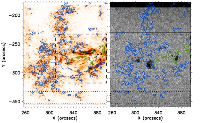
Figure 1: IRIS raster in Si iv 1402.8 Å (left, in reversed color table) and a 2832 Å continuum (right). The dashed lines indicate the region filled by clusters of cool transition region loops, while the dotted lines denote the region where the rest wavelength of S i 1401.5 Å is determined. The blue and green contours represent the HMI longitudinal magnetic flux density levels at $-$200 Mx cm^-2 and 200 Mx cm^-2 respectively.

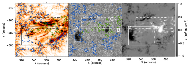
Figure 2: Loop region viewed in IRIS Si iv 1402.88 Å (left, in reversed color table), a 2832 Å continuum image (middle), and a HMI longitudinal magnetogram (right). The contours on the IRIS raster images correspond to HMI magnetic flux densities at $-$200 Mx cm^-2 (blue) and 200 Mx cm^-2 (green). “A” (with solid lines), “B” (with dotted lines) and “C” (with dashed lines) denote the three loop regions.

The IRIS observations were taken from 21:02 UT to 21:36 UT on 2013 December 27 targeting active region NOAA 11934. The spectral data were obtained by scanning the region from east to west in 400 steps with 0.35${}^{{}^{\prime\prime}}$step-size and 4 s exposure time. The pixel size along the slit is 0.17${}^{{}^{\prime\prime}}$. The field-of-view of the spectral data is 140${}^{{}^{\prime\prime}}$$\times$182${}^{{}^{\prime\prime}}$. The slit-jaw (SJ) images were recorded with a $\sim$10 s cadence and a pixel size of $0.17\times 0.17$ arcsec². The IRIS data analysed here are level-2 products, on which dark current removal, flat-field, geometrical distortion, orbital and thermal drift corrections have been applied. A spatial offset between images taken in different spectral lines and SJ images found in Huang et al. (2014b) is not present in this dataset. The new data production pipeline used after 2014 May should have performed well to handle all the calibration processes. In the present study, the raster scan using Si iv 1402.8 Å and the SJ images taken in the 1400 Å channel are used to study cool transition region loops found in the observed FOV. These loops are also visible in the C ii raster. However, C ii shows self-absorption well seen now at the IRIS high spectral resolution (see also e.g. Huang et al., 2014b), therefore it is not suitable for calculations of plasma parameters.

Figure 1 displays the radiance images of the IRIS spectral raster in the Si iv 1402.8 Å line and the continuum emission summed from 2831.74 Å to 2833.27 Å. This figure gives an overview of the solar features (cool loops, sunspots and pores etc.) observed in this region. A sub-region filled by cool transition region loops located on the right hand side of the field-of-view is seen in the Si iv image. A few sunspots and pores connecting the loop systems are visible in the continuum image.

Line-of-sight magnetograms taken by the Helioseismic and Magnetic Imager (HMI, Schou et al., 2012) with a 45 s cadence are also used in this study to determine the topology and evolution of the magnetic field of the region.

3 Wavelength calibration

In order to measure velocities in the transition region Si iv 1402.8 Å line, the rest wavelength was determined first. We applied an approach similar to the one proposed by Young et al. (2012) for Hinode/EIS hot lines. We first obtained the wavelength offset of Si iv 1402.8 Å relative to S i 1401.5Å averaged from a quiet-Sun (QS) dataset taken from 2013 October 9 at 23:26 UT to 2013 October 10 at 02:56 UT. We note that the QS dataset has been used in a study by Tian et al. (2014) showing excellent quality. Doppler-shifts of neutral lines are normally considered to be close to zero in the QS (see e.g. Brekke et al., 1997a). The field-of-view of the QS dataset covers various QS features, thus the average profile represents well the QS general characteristics. Next, an average profile of a quiet region in our dataset (marked by dotted lines in Figure 1) was produced to determine the S i 1401.5 Å line center. The quiet region is located away from the sunspots and covers a relatively large area (120${}^{{}^{\prime\prime}}$$\times$10${}^{{}^{\prime\prime}}$). Thus the S i 1401.5 Å can be considered as being at rest, i.e. at zero Doppler shift. The obtained S i 1401.5 Å line center with the offset given in the previous step added is then considered as the rest wavelength of Si iv 1402.8 Å. In this dataset, the rest wavelength of the line is found to be 1402.79 Å.

When calculating nonthermal velocities, one needs to know the ion formation temperature and the line broadening caused by instrumental effects (for details of the derivation, see Chae et al., 1998). In this study, we adopted the formation temperature given in the CHIANTI database (V7.1.3, Dere et al., 1997; Landi et al., 2013), i.e. 6.3$\times$10⁴ K. For instrumental broadening, we used a method that is commonly applied to SUMER data (see detailed description in Chae et al., 1998, and references therein). This method assumes that a spectral profile emitted by a neutral atom is not broadened by any nonthermal motions. Therefore, the broadening of an observed neutral line subtracted by its thermal part gives the instrumental broadening. In this study, we used the S i 1401.5 Å line obtained from the QS dataset mentioned above for this purpose. The instrumental broadening is found to be 57.3 mÅ at a full width at half maximum (FWHM). This value is relatively large compare to 31.8 mÅ given by the pre-flight measurements (see IRIS data user guide available on the web). However, it is a practical approach to obtain the instrumental broadening during the flight.

4 Results and discussion

In Figure 2, we show the IRIS Si iv 1402.8 Å, the continuum and the HMI magnetogram images of the loop region. Clusters of cool transition region loops can be clearly seen in the Si iv 1402.8 Å raster image (top-left panel). With the further aid of the 1400 Å SJ image sequence, we identified three groups of loops that evolve differently. They are denoted as A, B and C (Figure 2). We describe their physical properties, dynamics and evolution in great detail in the following sections.

4.1 Group A: cool transition region loop with one active footpoint

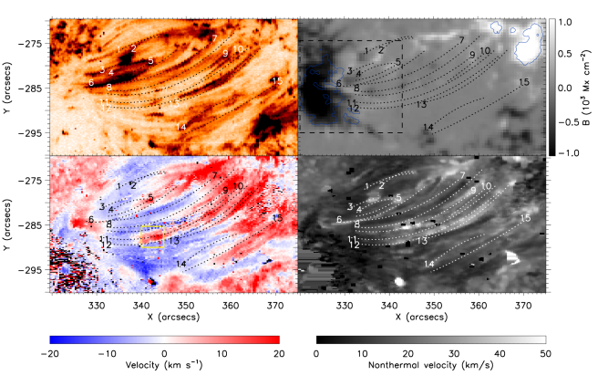
Figure 3: Radiance image in Si iv 1402.8 Å (top-left, in reversed color table), Doppler velocity image (bottom-left), nonthermal velocity image (bottom-right) and HMI magnetogram (top-right) of region “A”. The dotted lines mark 15 loops that were visually identified. The blue contours over-plotted on the magnetogram denote the emission of the IRIS 2832 Å continuum raster image. The yellow box on the Doppler image outlines the region where anti-parallel flows are seen. The box (dashed lines) on the magnetogram marks the area from which the magnetic cancellation rate is obtained.

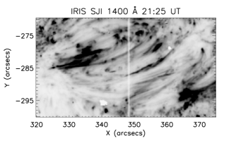
Figure 4: IRIS SJI 1400 Å snapshot of region “A”. The image is displayed in reversed color table. The white vertical line denotes the location of the spectrograph slit. (An animation is given online).

Figure 5: Doppler velocity variations along loops 7 (dotted line) and 11 (solid line) starting from their southern legs. The dashed line denotes a zero Doppler shift.

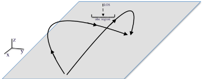
Figure 6: Configuration of two loops that can produce locally oppositely directed Doppler shifts when observed along the ‘LOS’ direction as shown in the figure.

Figure 7: Variation of nonthermal velocities along loops 7 (dotted line) and 11 (solid line) starting from their southern legs.

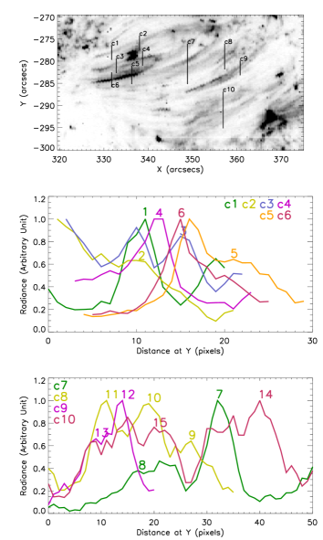
Figure 8: Lightcurves (middle and bottom panels) along the cuts given on the IRIS Si iv 1402.8 Å radiance image (black vertical lines, c1– c10 in the top panel) crossing 15 visually-identified loops. Peaks denoted with numbers mark loop locations.

The FOV containing group A is enlarged in Figure 3. In this region, we visually identified 15 loops (see Figure 3) using the Si iv radiance image and the SJ images (see Figure 4 and the online animation). The identification is based on cross-checking both the Si iv radiance image and the SJ images. Please note that this region is occupied by bundles of loops, many of which are clearly visible in the SJ images, though relatively weak in the Si iv radiance image (e.g. loops in the area below loop 12). Most of these loops do not show clear footpoints in the spectral data. In the IRIS SJ images, however, more loops with apparent plasma flows are visible (see online animation attached to Figure 4). Most of these loops end in nearby a region of two small sunspots (Figure 3 top-right panel). They appear to be rooted in weak magnetic features spread around the strong sunspot fields. The southern ends of these loops are located in a mixed-magnetic polarity region, while the northern ends are associated with a single polarity (positive) area. The apparent lengths of these loops vary from 10${}^{{}^{\prime\prime}}$($\sim$7 000 km) to 40${}^{{}^{\prime\prime}}$($\sim$30 000 km).

The Si iv Dopplergram of the region (bottom-left panel of Figure 3) clearly shows that the Doppler shifts gradually change from blue-shifted (negative values in the figure) in their southern legs to red-shifted (positive values in the figure) in their northern legs (except loop 6). This clearly indicates a plasma flow from the southern to northern legs of the loops. We note that a blue-shifted patch (red-shifted at the northern end) is present in the area between loop 12 and loop 15 where we did not identify any loops. This area is also occupied by loops that are clearly visible in the SJ images, and the blue/red-shifted patches should also represent siphon flows in loops in this region. The blue-shifts are about 10 km s^-1 at the southern ends, while the red-shifts are about 20 km s^-1 at the northern ends. Although the spectrometer slit scans the area only once, the Doppler velocities seem to be steady in the different loops scanned at different time. This indicates siphon flows in these loops that last at least for the duration of the observing period (i.e. $\sim$10 mins).

We also noticed that the velocity distributions along individual loops are different. Blue-shifts dominate along the apparent length of some loops (e.g. loops 8, 11), while red-shifts dominate in others (e.g. loops 7, 9 and 12). Figure 5 gives the variation of the Doppler velocities along loops 7 and 11. We can see that about 90% of the apparent length of loop 7 is blue-shifted, while about 80% of the apparent length of loop 11 is red-shifted. This velocity distribution leads to a localized region where “anti-parallel flows” are found (see e.g. the boxed region marked in the Dopplergram of Figure 3). Local anti-parallel plasma flows have been reported in Hi-C observations by Alexander et al. (2013), who suggest plasma flows in a highway manner. We further compared the phenomenon found here with that in Alexander et al. (2013). Our observation is based on Doppler velocity measurements that are different from the apparent velocities obtained in the Hi-C data. In the present case, the oppositely directed Doppler velocities do not suggest plasma flows in opposite directions as they converge to the same sign in the footpoints. In a localized region, they can simply result from the 3D geometry of the loops together with the projection effect. A possible geometry is drawn in Figure 6.

The nonthermal velocities of the region are shown in the bottom-right panel of Figure 3. In general, the nonthermal velocities do not significantly vary in major part of the loops. Figure 7 shows the variations of the nonthermal velocities along loops 7 and 11. Along loop 7, a dip is found at a distance of about 5${}^{{}^{\prime\prime}}$in the curve. After checking the selected loop path, we found that the first 5${}^{{}^{\prime\prime}}$of the loop seems to be affected by the activity occurring in loop 6. Appart from that, the nonthermal velocities of both loop 7 and loop 11 show a sharp increase at the first few arcseconds near their southern footpoints, and then fluctuate from 15  km s^-1 to 25  km s^-1. This implies that a dynamic process takes place in their southern legs where the energy and velocity of the plasma are gained. This is also supported by the mixed-polarity magnetic features in this footpoint region. Mixed-polarity magnetic features are usually associated with energetic events (e.g. coronal bright points, explosive events, X-ray jets and flares, Huang et al., 2012, 2014a, 2014b, and references therein). Nonthermal velocities of $\sim$20  km s^-1 found in these loops are consistent with the typical values obtained in the transition-region SUMER data (Chae et al., 1998). We, therefore, suggest that the loops in this group A are likely to have only one active footpoint at its southern end that is responsible for the siphon flows.

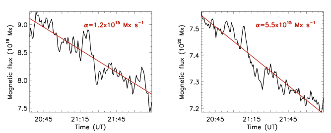
Figure 9: Variation of the positive (left panel) and negative (right panel) magnetic fluxes obtained in the southern ends of the loops (marked by black dashed lines on the magnetogram shown in Figure 3) in region “A”. The red lines are the linear fits of the curves. The magnetic cancellation rates derived from the fittings are given by the $\alpha$ values.

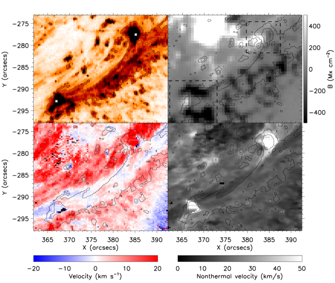
Figure 10: Radiance image in Si iv 1402.8 Å  (top-left, in reversed color table), a Doppler velocity image (bottom-left), a nonthermal velocity image (bottom-right) and a HMI magnetogram (top-right) of region “B”. The contours of the radiance image are over-plotted on all images. The loops inside the contours are better resolved in the SJ images shown in Figure 12. The asterisks on the radiance image mark the places where the spectral lines presented in Figure 11 are taken from. The dashed lines on the magnetogram mark the area from which the magnetic cancellation rate is obtained.

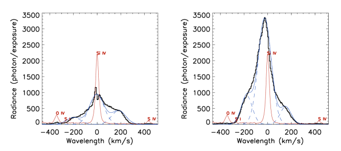
Figure 11: Examples of the Si iv 1402.8 Å profiles taken from the southern (left) and northern (right) footpoints of the loops in region B (asterisks in Figure 10). The blue solid lines are the resulting triple Gaussian fit. The blue dashed lines are the three Gaussian components. The average profiles from the region described in Section 3 are shown in red (increased 200 times). The identified emission lines are marked.

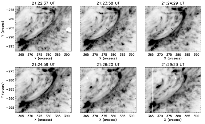
Figure 12: Evolution of the loops in region B seen in IRIS SJ 1400 Å  images (in reversed colour table). The dotted line in the image at 21:22:37 UT outlines a loop. Arrows denote the locations of the loops in the region. The white vertical line in the image at 21:29:23 UT is the IRIS spectrometer slit. (An animation is given online).

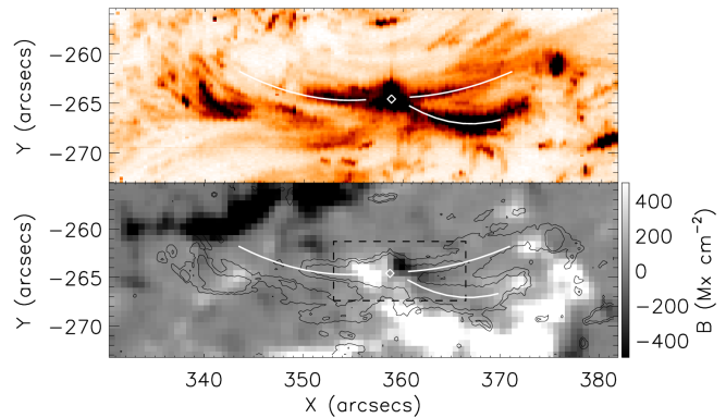
Figure 13: Radiance image in Si iv 1402.8 Å (top, in reversed color table) and a HMI magnetogram (bottom) of region “C”. The contours of the radiance image are over-plotted on the magnetogram. The diamond symbol denotes the conjunction of the two loop systems. Three loops identified from the radiance image are marked by white solid lines. The dashed lines on the magnetogram mark the area from which the magnetic cancellation rate is obtained.

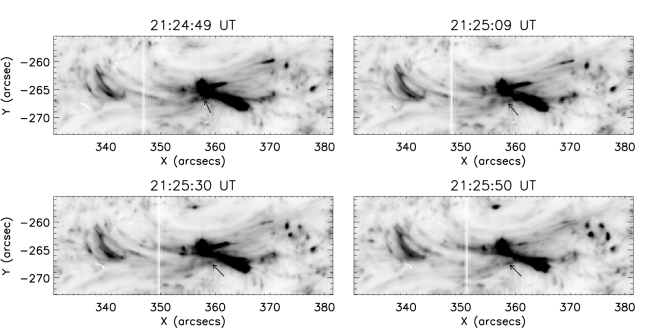
Figure 14: Evolution of the loops in region C seen in the IRIS SJ 1400 Å images (in reversed colour table). The arrows denote the evolution of a loop moving away from the active conjunction. (An animation is given online).

The unprecedented high spatial resolution of the IRIS images gives us an opportunity to measure the cross-sections of these loops. In the past, the instrumental resolution was one of the main issues for such measurements (Reale, 2014). In Figure 8 we show the Si iv 1402.8 Å emission along the cuts across the loops given in the top panel. The location of a loop is then determined by a peak in the lightcurve, while the dips at both sides determine the edges of the loop projection on the disk. If a loop is well isolated, its cross-section is then defined by the FWHM of the curve. One can see from Figure 8 that it is not possible to separate most of the loops from other features in the FOV. Therefore their cross-sections can not be measured due to the overlapping effect. From 15 loops, we could carry measurements for loops 1, 4 and 7 only. Their cross-sections are 4 pixels ($\sim$490 km), 3.1 pixels ($\sim$382 km), and 5.1 pixels ($\sim$626 km), respectively. Given that the cuts are not perpendicular to the loop, the real cross-section should be less than the obtained values. Although the cross-sections of the rest of the loops can not be measured accurately, a large number of them should have similar or even smaller sizes according to their appearances compared to loops 1, 4 and 7. In comparison with warm and hot loops measured by the Hi-C that are found to have cross-sections ranging from 300 km (Brooks et al., 2013) to 1 000 km (Peter et al., 2013), the cross sections measured in our data are close to lower limit of the Hi-C measurements. Loops forming at transition region temperatures seem to have finer scales than coronal loops.

Spectroscopic measurements bring important information that can help to understand the physical mechanism that heats and drives plasma flows along cool loops. We assume that the typical temperature of these loops is $\sim 6\times 10^{4}$ K, the loop length is $\sim 10^{4}$ km and the electron density is $\sim 10^{10}$ cm^-3 (a value representative of the transition region). The observed siphon flow field lasts for at least 10 mins, which is consistent with the picture where these loops are heated in a steady manner by an energy source in the blue-shifted footpoints (southern legs). Given that there are an infinite number of ways for prescribing the spatial heating profile, we, therefore, choose to focus on one mechanism where the heating derives from Alfvén waves (for details, see O’Neill & Li, 2005). The wave energy, originally in the low-frequency Magnetohydrodynamic regime, is turbulently cascaded towards high-frequencies until proton-cyclotron resonance comes into play, whereby the energy of the turbulently generated proton-cyclotron waves are absorbed by protons. Electrons are then heated via Coulomb collisions with protons. Assuming that the Alfvén waves are generated at locations in the chromosphere where the temperature is $2\times 10^{4}$ K, what is appealing in this mechanism is that $T_{M}$, the maximum temperature a loop acquires, depends only on the looplength $L$ and the imposed wave amplitude $\xi$. With $\xi$ being constrained by SOHO/SUMER measurements (e.g., Chae et al., 1998), the lowest value that $T_{M}$ attains depends only on $L$. An exhaustive parameter study (O’Neill & Li, 2005) suggests that $T_{M}$ for a loop length of $\sim 10^{4}$ km always exceeds $0.7$ MK, which is much higher than the formation temperature of Si iv. Lowering $\xi$ from its nominal value of $14$ km/s to $10$ km/s does not lower $T_{M}$ much. Introducing further complications such as the possibly unresolved magnetic twists actually makes $T_{M}$ even higher (Li & Li, 2006). We note that even within the class of models where Alfvén waves are the primary energy source for coronal heating, there are ways for dissipating the wave energy other than the parallel-cascade scenario adopted in O’Neill & Li (2005). For instance, van Ballegooijen et al. (2011) proposed that the turbulent cascade may proceed primarily in the lateral rather than in the mean-field direction as a result of the nonlinear interactions between counter-propagating Alfvén waves. While a definitive answer is still not available regarding how the loop temperatures and densities depend on loop lengths in this scenario, this loop-length dependence may well be different from what was found in O’Neill & Li (2005). In view of this, we conclude that the Alfvén wave heating mechanism described by O’Neill & Li (2005) is unlikely to reproduce the measured loops that emit strongly in Si iv. However, we cannot rule out the possibility that other steady heating mechanisms, such as the one by van Ballegooijen et al. (2011), may provide a satisfactory explanation for the physical properties of this set of cool transition region loops observed by IRIS.

Another mechanism that may account for the velocity field is the impulsive heating that is often invoked in interpreting warm loop observations (see Section 1). To discuss this aspect further, we note that three timescales are relevant, namely the electron thermal conduction timescale $\tau_{\mathrm{cond}}$, radiative cooling timescale $\tau_{\mathrm{rad}}$, and the timescale $\tau_{\mathrm{enth}}$ at which enthalpy flux plays a role. Let $n_{8}$, $T_{6}$, and $L_{9}$ denote the electron density in $10^{8}$ cm^-3, temperature in $10^{6}$ K, and loop length in $10^{9}$ cm, respectively. We then take $n_{8}=100$, $T_{6}=0.06$ and $L_{9}=1$ to be representative of the observed cool loops. With $\tau_{\mathrm{cond}}=160n_{8}L_{9}^{2}/T_{6}^{5/2}$ (Reale, 2014), one finds that $\tau_{\mathrm{cond}}\sim 10^{7}$ seconds. Likewise, one finds that $\tau_{\mathrm{rad}}\approx 40/(n_{8}T_{6})$ at the temperature range of interest, yielding $\tau_{\mathrm{rad}}\approx 7$ seconds. On the other hand, the enthalpy timescale may be approximated with the longitudinal sound transit time given that the flow speed is not too far from the sound speed ($140\sqrt{T_{6}}\approx 30$ km/s). This yields that $\tau_{\mathrm{enth}}\approx 70L_{9}/\sqrt{T_{6}}\approx 280$ seconds. As the most likely location where the heating pulses are generated are the southern ends, it then follows from the evaluation of the timescales that a single heating pulse cannot account for the loop measurements. Neither the electron heat conduction nor the enthalpy is able to redistribute the heat along the loop because their timescales are substantially longer than the radiative cooling time scale. Therefore a series of heating pulses is the most likely mechanism, and the total duration of these heating events should last longer than the enthalpy timescale (i.e. $\sim 5$ mins), and the temporal separation between two pulses should be substantially shorter than the radiative cooling timescale (i.e. $\sim 7$ secs).

One may now ask what constitutes a heating pulse. As discussed in Klimchuk (2006) and Parnell & De Moortel (2012), this pulse can be either AC (resonant wave absorption) or DC (nanoflares) in origin.

Resonant wave absorption is reasonable in this area because the loops are rooted in a sunspot area where masses of different modes of oscillations have been suggested and reported (see e.g. Marsch et al., 2004; Yuan et al., 2014, and references therein). By applying a wavelet analysis to various locations in these loops, we find no signature of oscillations. However, the wave scenario can not be ruled out because observational effects (such as overlapping, low temporal resolution) can be the reason that no periodicity is found in our analyses.

Nanoflares were first proposed by Parker (1988) as the most basic unit of impulsive energy release in the solar atmosphere. They are defined by the released total energy rather than any particular event. By definition the nanoflare energy is $\sim 10^{23}$ erg, i.e. $10^{9}$ times smaller than the flare energy ($10^{32}$ erg). It has been suggested that a nanoflare is the signature of small-scale magnetic reconnection occurring in the solar atmosphere (see e.g. Winebarger et al., 2002a; Cirtain et al., 2013). For these loops, the mixed-polarity magnetic features in the southern ends suggest that magnetic reconnection might take place in the area. We further investigated the magnetic flux in the southern footpoints. In Figure 9, we show the variation of the magnetic flux in this area from 20:30 UT to 22:13 UT. Magnetic cancellation is clearly present with rates of $1.2\times 10^{15}$ Mx s^-1 for the positive flux and $5.5\times 10^{15}$ Mx s^-1 for the negative flux. The cancellation rate for the negative flux is larger because the calculation includes the large sunspot that might cancel with the positive flux outside the selected box. High magnetic cancellation rates have been widely related to various energetic events, e.g. flares, jets, explosive events, etc. For comparison, the cancellation rates are about $8\times 10^{15}$ Mx s^-1 in footpoints of an active region outflow (Vanninathan et al., 2015), $5\times 10^{14}$ Mx s^-1 in an explosive event (Huang et al., 2014b) and X-ray jets (Huang et al., 2012), and $10^{16}$ Mx s^-1 in a GOES C4.3 flare (Huang et al., 2014a). Therefore, the $10^{15}$ Mx s^-1 cancellation rate suggests a significant magnetic energy release in the footpoints of these loops. Since the cancellation rate here is obtained from a large area that should include multiple energetic events, energy released in a single event might be less than that in one explosive event (i.e. $\sim 10^{24}$ erg, see e.g. Winebarger et al., 2002a). Unfortunately, the current data do not allow a quantitive analysis of the energy release in the region. An investigation using high-resolution vector magnetic field data and/or simulations could provide a deeper insight on the issue.

To conclude, the cool loops in group A are possibly heated by a series of heating pulses in their southern legs produced by magnetic reconnection. The magnetic reconnection scenario is strongly supported by the observed continuous magnetic flux cancellation. The magnetic energy is released in an intermittent manner with a cadence less than 7 s. The enthalpy flux associated with the sub-sonic flow plays an important role in constantly redistributing the heat deposited therein.

4.2 Group B: cool transition region loop with two active footpoints

Group B includes loops with compact brightenings in both footpoints (top-left panel of Figure 10, where the black patches marked by asterisk symbols are the footpoints of the loops), which are located in mixed-polarity magnetic flux regions (see top-right panel of Figure 10). The Doppler shifts (bottom-left panel of Figure 10) along these loops are very different from those in group A. No signature of siphon flows is recorded in the Doppler velocities. Instead, blue and red Doppler shifts ranging from $-5$  km s^-1 to 12  km s^-1 are distributed alternately along the loops. The nonthermal velocities of the region (bottom-right panel of Figure 10) clearly show large values in the footpoints where explosive-event line profiles are observed (see the discussion below). The nonthermal velocities are in the range from 10  km s^-1 to 25  km s^-1 with higher values at the two ends of the loops.

The footpoint regions of the loops are very dynamic, strongly suggesting that the energy sources for the loop heating are located there. We further investigated the Si iv 1402.8 Å line profiles in the region, and we found typical explosive-event line profiles in the footpoints (see the examples given in Figure 11). The line profiles suggest that bi-directional plasma flows with velocities of about 200  km s^-1 are produced. This type of line profiles has been suggested to be a signature of magnetic reconnection in the transition region (e.g. Innes et al., 1997; Huang et al., 2014b; Peter et al., 2014, among others). Magnetic cancellation is also found in the two footpoints of the loop group. The cancellation rates derived from the two boxed regions outlined in Figure 10 are found to be about $10^{15}$ Mx s^-1 indicating the release of a large amount of magnetic energy.

Explosive-event line profiles in both footpoints also imply that oppositely directed flows might take place. The small Doppler shifts found in the loops away from the footpoints might result from oppositely directed flows being canceled out in nearby loop strands. To investigate this possibility, we trace the temporal evolution of the loops seen in the IRIS SJ 1400 Å images (see online animation, Figure 12). We found that the group consists of multiple fine loop strands (see Figure 12, marked by arrows). Their footpoints are rooted in compact small areas. Two parallel loops are clearly seen at 21:26:20 UT (indicated with arrows). This again supports the possibility that anti-parallel flows in close-by loop strands cancel out to produce the detected Doppler velocities in the raster scan. We would like to note that the SJ images have higher spatial resolution in the solar X direction (0.17  arcsec/pixel) than the raster scan that is defined by the slit width (0.35 arcsec/pixel). Blue and red Doppler shifts appear along the loops suggesting that flows with one and the other direction are present.

4.3 Group C: interactions of two cool transition region loop systems

Group C consists of two loop systems, which are interacting with each other, and therefore show very dynamic evolution. The interaction occurs at the conjunction of the two of the footpoints of the loop systems (see the diamond symbol in Figure 13). The Si iv 1402.8 Å profiles in most pixels of the region are non-Gaussian. Explosive-event line profiles are seen all over in this area. This is also supported by the observed high rate of magnetic cancellation of about $3\times 10^{15}$ Mx s^-1. Magnetic reconnection possibly occurs between the two interacting loop systems. This kind of reconnection should generate a small-scale loop in the reconnection site which then submerges and a long loop connecting the two far ends. To further investigate this, we analyzed the temporal evolution of the region in the IRIS SJ 1400 Å  images (see Figure 14 and the attached animation). We observed a loop rising from the conjunction region (see the arrows in Figure 14), which is most likely one of the long loops formed during the reconnection process. This loop, however, disappears after 21:26 UT. It might have been heated to higher temperatures or the plasma has drained towards the footpoints. We also searched for signatures of heated loops in the 171 Å channel of the Atmospheric Imaging Assembly (AIA, Lemen et al., 2012), where the conjunction region is clearly visible. Because of the low resolution, we see some fuzzy cloud-like features rising from the conjunction area rather than any clear loop structures. A coronal imager with higher spatial resolution is essential to obtain a firm answer on this issue.

5 Summary and conclusions

In the present work, we have studied clusters of cool transition region loops in NOAA AR11934 observed by IRIS from 21:02 UT to 21:36 UT on 2013 December 27 at unprecedented resolution in the Si iv 1402.8 Å line. The analysed cool transition region loops are finely structured and have different dynamics and evolution. Three groups of loops were identified and studied in great detail.

The loops in group A are relatively stable. They are finely structured with cross-sections of about 382–626 km. Their southern legs are rooted in a mixed-magnetic polarity region near a small sunspot while their northern legs are associated with a single magnetic polarity. Possible siphon flows in these loops are suggested by the Si iv 1402.8 Å Doppler velocities that are gradually changing from about 10  km s^-1 blue-shifts in the southern legs to about 20  km s^-1 red-shifts in the northern ones. The nonthermal velocities in the major sections of the loops vary from 15  km s^-1 to 25  km s^-1, but increase in the southern ends. We concluded that these loops can not be heated by a steady energy release process and impulsive heating mechanism is required. The energy is possibly deposited in their southern ends where magnetic cancellation with a rate of $10^{15}$ Mx s^-1 indicates the release of significant magnetic energy. The magnetic energy is likely to be released impulsively by magnetic reconnection, and it is redistributed by the enthalpy flux carried by the siphon flows.

The loops in group B have two active footpoints seen in Si iv 1402.8 Å. Both footpoints are located in mixed-polarity regions. Small-scale magnetic reconnection events are found in the footpoints, which are witnessed by explosive-event line profiles with enhanced wings at about 200  km s^-1 Doppler shifts and magnetic cancellation with a rate of about $10^{15}$ Mx s^-1. These loops are possibly impulsively powered by small magnetic reconnection events occurring in the transition region. Doppler velocities along the loops reveal that blue and red Doppler-shifts ranging from $-$5  km s^-1 to 12  km s^-1 alternate along the loop. The nonthermal velocities vary from 10  km s^-1 to 25  km s^-1. These loops viewed in the SJ images show finer strands in which oppositely directed plasma flows might be present.

Group C is an excellent example of the interactions of two loop systems that have two end points rooted in the same region. This conjunction region is associated with a mixed-polarity magnetic flux and is very dynamic as witnessed by strong non-Gaussian Si iv line profiles. Magnetic cancellation with a rate of $3\times 10^{15}$ Mx s^-1 is found in the area. Explosive-event line profiles suggest that magnetic reconnection occurs between these two loop systems.

In summary, cool transition region loops differ a lot from warm and hot loops. They are finely structured, more dynamic and diverse. Impulsive heating involving magnetic reconnection is the most plausible heating mechanism. Future numerical studies are required to fully understand the physics of cool loops and their role in coronal heating.

References

- Alexander et al. (2013) Alexander, C. E., Walsh, R. W., Régnier, S., et al. 2013, ApJ, 775, L32
- Brekke et al. (1997a) Brekke, P., Hassler, D. M., & Wilhelm, K. 1997a, Sol. Phys., 175, 349
- Brekke et al. (1997b) Brekke, P., Kjeldseth-Moe, O., & Harrison, R. A. 1997b, Sol. Phys., 175, 511
- Brooks et al. (2013) Brooks, D. H., Warren, H. P., Ugarte-Urra, I., & Winebarger, A. R. 2013, ApJ, 772, L19
- Cadavid et al. (2014) Cadavid, A. C., Lawrence, J. K., Christian, D. J., Jess, D. B., & Nigro, G. 2014, ApJ, 795, 48
- Cargill & Klimchuk (2004) Cargill, P. J., & Klimchuk, J. A. 2004, ApJ, 605, 911
- Chae et al. (1998) Chae, J., Schühle, U., & Lemaire, P. 1998, ApJ, 505, 957
- Chae et al. (2000) Chae, J., Wang, H., Qiu, J., Goode, P. R., & Wilhelm, K. 2000, ApJ, 533, 535
- Cirtain et al. (2013) Cirtain, J. W., Golub, L., Winebarger, A. R., et al. 2013, Nature, 493, 501
- De Pontieu et al. (2014) De Pontieu, B., Title, A. M., Lemen, J. R., et al. 2014, Sol. Phys., 289, 2733
- Del Zanna & Mason (2003) Del Zanna, G., & Mason, H. E. 2003, A&A, 406, 1089
- Dere et al. (1997) Dere, K. P., Landi, E., Mason, H. E., Monsignori Fossi, B. C., & Young, P. R. 1997, A&AS, 125, 149
- Di Giorgio et al. (2003) Di Giorgio, S., Reale, F., & Peres, G. 2003, A&A, 406, 323
- Dowdy (1993) Dowdy, Jr., J. F. 1993, ApJ, 411, 406
- Dowdy et al. (1986) Dowdy, Jr., J. F., Rabin, D., & Moore, R. L. 1986, Sol. Phys., 105, 35
- Doyle et al. (2006) Doyle, J. G., Taroyan, Y., Ishak, B., Madjarska, M. S., & Bradshaw, S. J. 2006, A&A, 452, 1075
- Feldman (1983) Feldman, U. 1983, ApJ, 275, 367
- Feldman (1987) —. 1987, ApJ, 320, 426
- Feldman (1998) —. 1998, ApJ, 507, 974
- Feldman et al. (2001) Feldman, U., Dammasch, I. E., & Wilhelm, K. 2001, ApJ, 558, 423
- Fletcher et al. (2014) Fletcher, L., Cargill, P. J., Antiochos, S. K., & Gudiksen, B. V. 2014, Space Sci. Rev., arXiv:1412.7378
- Fludra et al. (1997) Fludra, A., Brekke, P., Harrison, R. A., et al. 1997, Sol. Phys., 175, 487
- Huang et al. (2012) Huang, Z., Madjarska, M. S., Doyle, J. G., & Lamb, D. A. 2012, A&A, 548, A62
- Huang et al. (2014a) Huang, Z., Madjarska, M. S., Koleva, K., et al. 2014a, A&A, 566, A148
- Huang et al. (2014b) Huang, Z., Madjarska, M. S., Xia, L., et al. 2014b, ApJ, 797, 88
- Innes et al. (1997) Innes, D. E., Inhester, B., Axford, W. I., & Wilhelm, K. 1997, Nature, 386, 811
- Kjeldseth-Moe & Brekke (1998) Kjeldseth-Moe, O., & Brekke, P. 1998, Sol. Phys., 182, 73
- Klimchuk (2006) Klimchuk, J. A. 2006, Sol. Phys., 234, 41
- Klimchuk (2009) Klimchuk, J. A. 2009, in Astronomical Society of the Pacific Conference Series, Vol. 415, The Second Hinode Science Meeting: Beyond Discovery-Toward Understanding, ed. B. Lites, M. Cheung, T. Magara, J. Mariska, & K. Reeves, 221
- Landi et al. (2013) Landi, E., Young, P. R., Dere, K. P., Del Zanna, G., & Mason, H. E. 2013, ApJ, 763, 86
- Lemen et al. (2012) Lemen, J. R., Title, A. M., Akin, D. J., et al. 2012, Sol. Phys., 275, 17
- Li & Li (2006) Li, B., & Li, X. 2006, Royal Society of London Philosophical Transactions Series A, 364, 533
- Marsch et al. (2004) Marsch, E., Wiegelmann, T., & Xia, L. D. 2004, A&A, 428, 629
- O’Neill & Li (2005) O’Neill, I., & Li, X. 2005, A&A, 435, 1159
- Parker (1988) Parker, E. N. 1988, ApJ, 330, 474
- Parnell & De Moortel (2012) Parnell, C. E., & De Moortel, I. 2012, Royal Society of London Philosophical Transactions Series A, 370, 3217
- Peter et al. (2013) Peter, H., Bingert, S., Klimchuk, J. A., et al. 2013, A&A, 556, A104
- Peter et al. (2014) Peter, H., Tian, H., Curdt, W., et al. 2014, Science, 346, C315
- Reale (2014) Reale, F. 2014, Living Reviews in Solar Physics, 11, 4
- Sasso et al. (2012) Sasso, C., Andretta, V., Spadaro, D., & Susino, R. 2012, A&A, 537, A150
- Schou et al. (2012) Schou, J., Scherrer, P. H., Bush, R. I., et al. 2012, Sol. Phys., 275, 229
- Spadaro et al. (2000) Spadaro, D., Lanzafame, A. C., Consoli, L., et al. 2000, A&A, 359, 716
- Teriaca et al. (2004) Teriaca, L., Banerjee, D., Falchi, A., Doyle, J. G., & Madjarska, M. S. 2004, A&A, 427, 1065
- Tian et al. (2014) Tian, H., DeLuca, E. E., Cranmer, S. R., et al. 2014, Science, 346, A315
- Tripathi et al. (2009) Tripathi, D., Mason, H. E., Dwivedi, B. N., del Zanna, G., & Young, P. R. 2009, ApJ, 694, 1256
- Tripathi et al. (2010) Tripathi, D., Mason, H. E., & Klimchuk, J. A. 2010, ApJ, 723, 713
- Ugarte-Urra & Warren (2014) Ugarte-Urra, I., & Warren, H. P. 2014, ApJ, 783, 12
- Ugarte-Urra et al. (2009) Ugarte-Urra, I., Warren, H. P., & Brooks, D. H. 2009, ApJ, 695, 642
- van Ballegooijen et al. (2011) van Ballegooijen, A. A., Asgari-Targhi, M., Cranmer, S. R., & DeLuca, E. E. 2011, ApJ, 736, 3
- Vanninathan et al. (2015) Vanninathan, K., Madjarska, M. S., Galsgaard, K., Huang, Z., & Doyle, J. G. 2015, A&A, submitted
- Viall & Klimchuk (2011) Viall, N. M., & Klimchuk, J. A. 2011, ApJ, 738, 24
- Warren et al. (2010) Warren, H. P., Winebarger, A. R., & Brooks, D. H. 2010, ApJ, 711, 228
- Warren et al. (2003) Warren, H. P., Winebarger, A. R., & Mariska, J. T. 2003, ApJ, 593, 1174
- Winebarger et al. (2013) Winebarger, A., Tripathi, D., Mason, H. E., & Del Zanna, G. 2013, ApJ, 767, 107
- Winebarger et al. (2002a) Winebarger, A. R., Emslie, A. G., Mariska, J. T., & Warren, H. P. 2002a, ApJ, 565, 1298
- Winebarger et al. (2011) Winebarger, A. R., Schmelz, J. T., Warren, H. P., Saar, S. H., & Kashyap, V. L. 2011, ApJ, 740, 2
- Winebarger et al. (2002b) Winebarger, A. R., Warren, H., van Ballegooijen, A., DeLuca, E. E., & Golub, L. 2002b, ApJ, 567, L89
- Winebarger & Warren (2005) Winebarger, A. R., & Warren, H. P. 2005, ApJ, 626, 543
- Young et al. (2012) Young, P. R., O’Dwyer, B., & Mason, H. E. 2012, ApJ, 744, 14
- Yuan et al. (2014) Yuan, D., Nakariakov, V. M., Huang, Z., et al. 2014, ApJ, 792, 41