Strong Asymptotics of Hermite-Padé Approximants for Angelesco Systems

Abstract.

In this work type II Hermite-Padé approximants for a vector of Cauchy transforms of smooth Jacobi-type densities are considered. It is assumed that densities are supported on mutually disjoint intervals (an Angelesco system with complex weights). The formulae of strong asymptotics are derived for any ray sequence of multi-indices.

1   Introduction

Let $\vec{f}=(f_{1},\ldots,f_{p})$, $p\in\mathbb{N}$, be a vector of germs of holomorphic functions at infinity. Given a multi-index $\vec{n}\in\mathbb{N}^{p}$, Hermite-Padé approximant to $\vec{f}$ associated with $\vec{n}$, is a vector of rational functions

(1) $$[\>\vec{n}\>]_{\vec{f}}:=\left(P_{\vec{n}}^{(1)}/Q_{\vec{n}},\ldots,P_{\vec{n}}^{(p)}/Q_{\vec{n}}\right)$$

such that

(2) $$\left\{\begin{array}[]{l}\displaystyle\mathsf{deg}\big{(}Q_{\vec{n}}\big{)}=|\>\vec{n}\>|:=n_{1}+\cdots+n_{p},\vskip 6.0pt plus 2.0pt minus 2.0pt\\ \displaystyle R_{\vec{n}}^{(i)}(z):=\left(Q_{\vec{n}}f_{i}-P_{\vec{n}}^{(i)}\right)(z)=\mathcal{O}\left(z^{-(n_{i}+1)}\right)\quad\text{as}\quad z\to\infty,\quad i\in\{1,\ldots,p\}.\end{array}\right.$$

It is quite simple to see that $[\>\vec{n}\>]_{\vec{f}}$ always exists since (2) can be rewritten as a linear system that has more unknowns than equations with coefficients coming from the Laurent expansions of $f_{i}$’s at infinity. Hence, $Q_{\vec{n}}$ is never identically zero and, in what follows, we normalize $Q_{\vec{n}}$ to be monic.

The vector $\vec{f}$ is called an Angelesco system if

(3) $$f_{i}(z)=\int\frac{\mathrm{d}\sigma_{i}(t)}{t-z},\qquad i\in\{1,\ldots,p\},$$

where $\sigma_{i}$’s are positive measures on the real line with mutually disjoint convex hulls of their supports, i.e., $[a_{j},b_{j}]\cap[a_{k},b_{k}]=\varnothing$ for $j\neq k$ where $[a_{i},b_{i}]$ is the smallest interval containing $\mathsf{supp}(\sigma_{i})$. Hermite-Padé approximants to such systems were initially considered by Angelesco [1] and later by Nikishin [23, 24]. The beauty of system (3) is that $Q_{\vec{n}}$, the denominator of $[\>\vec{n}\>]_{\vec{f}}$, turns out to be a multiple orthogonal polynomial satisfying

(4) $$\int Q_{\vec{n}}(x)x^{k}\mathrm{d}\sigma_{i}(x)=0,\qquad k\in\{0,\ldots,n_{i}-1\},\quad i\in\{1,\ldots,p\}.$$

When $p=1$, Hermite-Padé approximant $[\>\vec{n}\>]_{\vec{f}}$ specializes to the diagonal Padé approximant, quite often denoted by $[n/n]_{f}$. It was shown by Markov [20] that if $f$ is of the form (3) (now called a Markov function), then $[n/n]_{f}$ converge to $f$ locally uniformly outside of $[a,b]$. Moreover, see [29, Thm. 6.1.6], it holds that

(5) $$\left\{\begin{array}[]{l}\displaystyle\lim_{n\to\infty}n^{-1}\log\big{|}f-[n/n]_{f}\big{|}\leq-2\big{(}\ell-V^{\omega}\big{)}\vskip 6.0pt plus 2.0pt minus 2.0pt\\ \displaystyle\lim_{n\to\infty}n^{-1}\log|Q_{n}|=-V^{\omega}\end{array}\right.$$

locally uniformly in $\overline{\mathbb{C}}\setminus[a,b]$, where $V^{\omega}(z):=-\int\log|z-t|\mathrm{d}\omega(t)$ is the logarithmic potential of $\omega$, while the measure $\omega$ and the constant $\ell$ are the unique solutions of the min/max problem:

(6) $$\ell:=\min_{x\in[a,b]}V^{\omega}(x)~{}=\max_{\nu\in M_{1}(a,b)}\min_{x\in[a,b]}V^{\nu}(x),$$

where $M_{c}(a,b)$ is the collection of all positive Borel measures of mass $c$ supported on $[a,b]$. In fact, it also holds that $\omega$ is the equilibrium distribution and $\ell$ is the Robin’s constant for the interval $[a,b]$. That is, $\omega$ is the unique measure on $[a,b]$ that solves the energy minimization problem:

(7) $$I[\omega]=\min_{\nu\in M_{1}(a,b)}I[\nu],\quad\quad\ell=I[\omega],$$

where $I[\nu]:=-\int\int\log|z-t|\mathrm{d}\nu(t)\mathrm{d}\nu(z)=\int V^{\nu}\mathrm{d}\nu$ is the logarithmic energy of $\nu$ (for the notions of logarithmic potential theory we use [27] and [28] as primary references).

It easily follows from (6)–(7) and properties of the superharmonic functions that

(8) $$\left\{\begin{array}[]{l}\ell-V^{\omega}\equiv 0\quad\text{on}\quad[a,b],\vskip 6.0pt plus 2.0pt minus 2.0pt\\ \ell-V^{\omega}>0\quad\text{in}\quad\overline{\mathbb{C}}\setminus[a,b].\end{array}\right.$$

Hence, the diagonal Padé approximants $[n/n]_{f}$ do indeed converge to $f$ locally uniformly in $\overline{\mathbb{C}}\setminus[a,b]$. Moreover, if $\sigma$ is a regular measure in the sense of Stahl and Totik [29, Sec. 3.1] (in particular, $\sigma^{\prime}>0$ almost everywhere on $[a,b]$ implies regularity), then the inequality in (5) can be replaced by equality.

The above results were extended by Gonchar and Rakhmanov [15] to Hermite-Padé approximants for Angelesco systems when multi-indices are such that

(9) $$n_{i}=c_{i}|\>\vec{n}\>|+o\left(|\>\vec{n}\>|\right),\qquad\vec{c}=(c_{1},\ldots,c_{p})\in\big{(}0,1)^{p},\quad|\>\vec{c}\>|=1,$$

as $|\>\vec{n}\>|\to\infty$, and the measures $\sigma_{i}$ satisfy $\sigma_{i}^{\prime}>0$ almost everywhere on $[a_{i},b_{i}]$, $i\in\{1,\ldots,p\}$. The formulae for the errors of approximation are similar in appearance to (5) with measures coming not from a scalar but from a vector minimum energy problem. To describe it, define

$$M_{\vec{c}}\big{(}\{a_{i},b_{i}\}_{1}^{p}\big{)}:=\big{\{}\vec{\nu}=(\nu_{1},\ldots,\nu_{p}):~{}\nu_{i}\in M_{c_{i}}(a_{i},b_{i}),~{}i\in\{1,\ldots,p\}\big{\}}.$$

Then it is known that there exists the unique vector of measures $\vec{\omega}\in M_{\vec{c}}\big{(}\{a_{i},b_{i}\}_{1}^{p}\big{)}$ such that

(10) $$I[\>\vec{\omega}\>]=\min_{\nu\in M_{\vec{c}}(\{a_{i},b_{i}\}_{1}^{p})}I[\>\vec{\nu}\>],\qquad I[\>\vec{\nu}\>]:=\sum_{i=1}^{p}\bigg{(}2I[\nu_{i}]+\sum_{k\neq i}I[\nu_{i},\nu_{k}]\bigg{)},$$

where $I[\nu_{i},\nu_{k}]:=-\int\int\log|z-t|\mathrm{d}\nu_{i}(t)\mathrm{d}\nu_{k}(z)$. The measures $\omega_{i}$ might no longer be supported on the whole intervals $[a_{i},b_{i}]$ (the so-called pushing effect), but in general it holds that

(11) $$\mathsf{supp}(\omega_{i})=[a_{\vec{c},i},b_{\vec{c},i}]\subseteq[a_{i},b_{i}],\qquad i\in\{1,\ldots,p\}.$$

Let $W^{\vec{\nu}}$ be a function on $\bigcup_{i=1}^{p}[a_{i},b_{i}]$ such that its restriction to $[a_{i},b_{i}]$ is equal to $V^{\nu_{i}+\nu}$ where $\nu=\sum_{i=1}^{p}\nu_{i}$ is a probability measure such that $\nu_{|[a_{i},b_{i}]}=\nu_{i}$. Exactly as in (6), the equilibrium vector measure $\vec{\omega}$ can be characterized by the following property: if

(12) $$\min_{x\in[a_{i},b_{i}]}W^{\vec{\nu}}(x)\geq\min_{x\in[a_{i},b_{i}]}W^{\vec{\omega}}(x)=:\ell_{i}$$

simultaneously for all $i\in\{1,\ldots,p\}$ for some $\vec{\nu}\in M_{\vec{c}}\big{(}\{a_{i},b_{i}\}_{1}^{p}\big{)}$, then $\vec{\nu}=\vec{\omega}$.

Having all the definitions at hand, we can formulate the main result of [15], which states that

(13) $$\left\{\begin{array}[]{l}\displaystyle\lim_{|\>\vec{n}\>|\to\infty}|\>\vec{n}\>|^{-1}\log\big{|}f_{i}-P_{\vec{n}}^{(i)}/Q_{\vec{n}}\big{|}=-\big{(}\ell_{i}-V^{\omega_{i}+\omega}\big{)},\quad i\in\{1,\ldots,p\},\vskip 6.0pt plus 2.0pt minus 2.0pt\\ \displaystyle\lim_{|\>\vec{n}\>|\to\infty}|\>\vec{n}\>|^{-1}\log|Q_{\vec{n}}|=-V^{\omega}\end{array}\right.$$

locally uniformly in $\overline{\mathbb{C}}\setminus\bigcup_{i=1}^{p}[a_{i},b_{i}]$. Even though (13) looks exactly as (5), the convergence properties of the approximants are not as straightforward. Indeed, it is a direct consequence of the pushing effect ($[a_{\vec{c},i},b_{\vec{c},i}]\subsetneq[a_{i},b_{i}]$), when it occurs, of course, that the first relation in (8) is replaced now by

(14) $$\left\{\begin{array}[]{l}\ell_{i}-V^{\omega_{i}+\omega}\equiv 0\quad\text{on}\quad[a_{\vec{c},i},b_{\vec{c},i}],\vskip 6.0pt plus 2.0pt minus 2.0pt\\ \ell_{i}-V^{\omega_{i}+\omega}<0\quad\text{on}\quad[a_{i},b_{i}]\setminus[a_{\vec{c},i},b_{\vec{c},i}].\end{array}\right.$$

Further, set

(15) $$\left\{\begin{array}[]{lll}D_{i}^{+}&:=&\displaystyle\big{\{}z:~{}\ell_{i}-V^{\omega_{i}+\omega}(z)>0\big{\}},\vskip 6.0pt plus 2.0pt minus 2.0pt\\ D_{i}^{-}&:=&\displaystyle\big{\{}z:~{}\ell_{i}-V^{\omega_{i}+\omega}(z)<0\big{\}}.\end{array}\right.$$

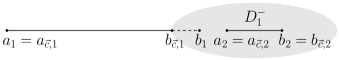
Figure 1. Schematic representation of the pushing effect in the case of 2 intervals (in Proposition 3 we shall show that this is the only possible situation for pushing effect in the case of 2 intervals; this is also explained in [15]). The shaded region is the divergence domain $D_{1}^{-}$ while $D_{2}^{-}=\varnothing$.

Properties of the logarithmic potentials immediately imply that $D_{i}^{+}$ is an unbounded domain. This is exactly the domain in which the approximants $P_{\vec{n}}^{(i)}/Q_{\vec{n}}$ converge to $f_{i}$ locally uniformly, while $D_{i}^{-}$ is a bounded open set on which the approximants diverge to infinity. This set can be empty or not. The latter situation necessarily happens when $[a_{\vec{c},i},b_{\vec{c},i}]\subsetneq[a_{i},b_{i}]$ as can be clearly seen from the second line in (14); however, the pushing effect is not necessary for the divergence set to exist.

The result of Gonchar and Rakhmanov (13) belongs to the realm of the so called weak asymptotics as to distinguish from strong asymptotics in which one establishes the existence of and identifies the limits

(16) $$\left\{\begin{array}[]{l}\displaystyle\lim_{|\>\vec{n}\>|\to\infty}\left(\log\big{|}f_{i}-P_{\vec{n}}^{(i)}/Q_{\vec{n}}\big{|}+|\>\vec{n}\>|\big{(}\ell_{i}-V^{\omega_{i}+\omega}\big{)}\right),\vskip 6.0pt plus 2.0pt minus 2.0pt\\ \displaystyle\lim_{|\>\vec{n}\>|\to\infty}\big{(}\log|Q_{\vec{n}}|+|\>\vec{n}\>|V^{\omega}\big{)}.\end{array}\right.$$

Not surprisingly, the first result completely answering the previous question was obtained for Padé approximants ($p=1$) by Szegő. He proved that limit (16) takes place exactly when $\sigma^{\prime}$ satisfied $\int\log\sigma^{\prime}\mathrm{d}\omega>-\infty$, which is now known as Szegő condition. The analog of the Szegő theorem for true Hermite-Padé approximants was proven by Aptekarev [2] when $p=2$ and the multi-indices are diagonal ($\vec{n}=(n,n)$) with indications how one could carry the approach to any $p>1$. A rigorous proof for any $p$ and diagonal multi-indices was completed by Aptekarev and Lysov [4] for systems $\vec{f}$ of Markov functions generated by cyclic graphs (the so called generalized Nikishin systems), of which Angelesco systems are a particular example. The restriction on the measures $\sigma_{i}$ is more stringent in [4], as it is required that

(17) $$\sigma_{i}^{\prime}(x)=h_{i}(x)(x-a_{i})^{\alpha_{i}}(b_{i}-x)^{\beta_{i}},\qquad\alpha_{i},\beta_{i}>-1,$$

and $h_{i}$ is holomorphic and non-vanishing in some neighborhood of $[a_{i},b_{i}]$.

From the approximation theory point of view it is not natural to require the measures $\sigma_{i}$ to be positive (as well as to be supported on the real line, but we shall not dwell on this point here). In the case of Padé approximants it was Nuttall [25] who proved the existence of and identified the limit in (16) for the set up (3) and (17) with $\alpha=\beta=-1/2$ and $h$ being Hölder continuous, non-vanishing, and complex-valued on $[a,b]$. The proof of Szegő theorem for any parameters $\alpha,\beta>-1$ and $h$ complex-valued, holomorphic, and non-vanishing around $[a,b]$ follows from Aptekarev [3] (this result was not the main focus of [3], there weighed approximation on one-arc S-contours was considered), and the condition of holomorphy of $h$ was relaxed by Baratchart and the author in [5], where $h$ is taken from a fractional Sobolev space that depends on the parameters $\alpha,\beta$ (again, the main focus of [5] was weighted (multipoint) Padé approximation on one-arc S-contours). The goal of this work is to extend the results of [4] to Angelesco systems with complex weights and Hermite-Padé approximants corresponding to multi-indices as in (9).

2   Main Results

From now on, we fix a system of mutually disjoint intervals $\big{\{}[a_{i},b_{i}]\big{\}}_{i=1}^{p}$ and a vector $\vec{c}\in(0,1)^{p}$ such that $|\>\vec{c}\>|=1$. We further denote by

$$\vec{\omega}=(\omega_{1},\ldots,\omega_{p}),\quad\omega:=\sum_{i=1}^{p}\omega_{i},\quad\mathsf{supp}(\omega_{i})=\big{[}a_{\vec{c},i},b_{\vec{c},i}\big{]}\subseteq[a_{i},b_{i}],$$

the equilibrium vector measure minimizing the energy functional (10).

To describe the forthcoming results we shall need a $(p+1)$-sheeted compact Riemann surface, say $\boldsymbol{\mathfrak{R}}$, that we realize in the following way. Take $p+1$ copies of $\overline{\mathbb{C}}$. Cut one of them along the union $\bigcup_{i=1}^{p}\big{[}a_{\vec{c},i},b_{\vec{c},i}\big{]}$, which henceforth is denoted by $\boldsymbol{\mathfrak{R}}^{(0)}$. Each of the remaining copies cut along only one interval $\big{[}a_{\vec{c},i},b_{\vec{c},i}\big{]}$ so that no two copies have the same cut and denote them by $\boldsymbol{\mathfrak{R}}^{(i)}$. To form $\boldsymbol{\mathfrak{R}}$, take $\boldsymbol{\mathfrak{R}}^{(i)}$ and glue the banks of the cut $\big{[}a_{\vec{c},i},b_{\vec{c},i}\big{]}$ crosswise to the banks of the corresponding cut on $\boldsymbol{\mathfrak{R}}^{(0)}$.

It can be easily verified that thus constructed Riemann surface has genus 0. Denote by $\pi$ the natural projection from $\boldsymbol{\mathfrak{R}}$ to $\overline{\mathbb{C}}$. We shall denote by ${\boldsymbol{z}},{\boldsymbol{w}},{\boldsymbol{x}},{\boldsymbol{e}}$ generic points on $\boldsymbol{\mathfrak{R}}$ with natural projections $z,w,x,e$. We also shall employ the notation $z^{(i)}$ for a point on $\boldsymbol{\mathfrak{R}}^{(i)}$ with $\pi(z^{(i)})=z$. This notation is well defined everywhere outside of the cycles $\boldsymbol{\Delta}_{i}:=\boldsymbol{\mathfrak{R}}^{(0)}\cap\boldsymbol{\mathfrak{R}}^{(i)}$. Clearly, $\pi(\boldsymbol{\Delta}_{i})=\big{[}a_{\vec{c},i},b_{\vec{c},i}\big{]}$. It also will be convenient to denote by $\boldsymbol{a}_{\vec{c},i}$ and $\boldsymbol{b}_{\vec{c},i}$ the branch points of $\boldsymbol{\mathfrak{R}}$ with respective projections $a_{\vec{c},i}$ and $b_{\vec{c},i}$, $i\in\{1,\ldots,p\}$.

Unfortunately, to be able to handle general multi-indices of form (9), one Riemann surface is not sufficient. Let $\vec{n}\in\mathbb{N}^{p}$. Denote by

$$\vec{\omega}_{\vec{n}}=(\omega_{\vec{n},1},\ldots,\omega_{\vec{n},p}),\quad\omega_{\vec{n}}:=\sum_{i=1}^{p}\omega_{\vec{n},i},\quad\mathsf{supp}(\omega_{\vec{n},i})=\big{[}a_{\vec{n},i},b_{\vec{n},i}\big{]}\subseteq[a_{i},b_{i}],$$

the equilibrium vector measure minimizing the energy functional (10) where $\vec{c}$ is replaced by the vector $\big{(}n_{1}/|\>\vec{n}\>|,\ldots,n_{p}/|\>\vec{n}\>|\big{)}$. The surface $\boldsymbol{\mathfrak{R}}_{\vec{n}}$ is defined absolutely analogously to $\boldsymbol{\mathfrak{R}}$. Notation $\boldsymbol{\Delta}_{\vec{n},i}$, $\boldsymbol{a}_{\vec{n},i}$, and $\boldsymbol{b}_{\vec{n},i}$, $i\in\{1,\ldots,p\}$, is self-evident now.

Since each $\boldsymbol{\mathfrak{R}}_{\vec{n}}$ has genus zero, one can arbitrarily prescribe zero/pole multisets of rational functions on $\boldsymbol{\mathfrak{R}}_{\vec{n}}$ as long as the multisets have the same cardinality. Thus, given a multi-index $\vec{n}$, we shall denote $\Phi_{\vec{n}}$ a rational function on $\boldsymbol{\mathfrak{R}}_{\vec{n}}$ which is non-zero and finite everywhere on $\boldsymbol{\mathfrak{R}}_{\vec{n}}\setminus\bigcup_{k=0}^{p}\big{\{}\infty^{(k)}\big{\}}$, has a pole of order $|\>\vec{n}\>|$ at $\infty^{(0)}$, a zero of multiplicity $n_{i}$ at each $\infty^{(i)}$, and satisfies

(18) $$\prod_{k=0}^{p}\Phi_{\vec{n}}\big{(}z^{(k)}\big{)}\equiv 1.$$

Normalization (18) is possible since the function $\log\prod_{k=0}^{p}\big{|}\Phi_{\vec{n}}\big{(}z^{(k)}\big{)}\big{|}$ extends to a harmonic function on $\mathbb{C}$ which has a well defined limit at infinity. Hence, it is constant. Therefore, if (18) holds at one point, it holds throughout $\overline{\mathbb{C}}$. The importance of the function $\Phi_{\vec{n}}$ to our analysis lies in the following proposition.

Proposition 1.

With the above notation, it holds that

$$\frac{1}{|\>\vec{n}\>|}\log\big{|}\Phi_{\vec{n}}({\boldsymbol{z}})\big{|}=\left\{\begin{array}[]{ll}-V^{\omega_{\vec{n}}}(z)+\frac{1}{p+1}\sum_{k=1}^{p}\ell_{\vec{n},k},&{\boldsymbol{z}}\in\boldsymbol{\mathfrak{R}}_{\vec{n}}^{(0)},\vskip 6.0pt plus 2.0pt minus 2.0pt\\ V^{\omega_{\vec{n},i}}(z)-\ell_{\vec{n},i}+\frac{1}{p+1}\sum_{k=1}^{p}\ell_{\vec{n},k},&{\boldsymbol{z}}\in\boldsymbol{\mathfrak{R}}_{\vec{n}}^{(i)},\quad i\in\{1,\ldots,p\}.\end{array}\right.$$

If a sequence $\big{\{}\vec{n}\big{\}}$ satisfies (9), then the measures $\omega_{\vec{n}}$ converge to $\omega$ in the weak^∗ topology of measures as $|\>\vec{n}\>|\to\infty$ (in particular, this implies that $\ell_{\vec{n},i}\to\ell_{i}$, $a_{\vec{n},i}\to a_{\vec{c},i}$, and $b_{\vec{n},i}\to b_{\vec{c},i}$). Moreover, it holds that $V^{\omega_{\vec{n},i}}\to V^{\omega_{i}}$ uniformly on compact subsets of $\mathbb{C}$ for each $i\in\{1,\ldots,p\}$.

It immediately follows from Proposition 1 that

(19) $$\frac{1}{|\>\vec{n}\>|}\log\left|\frac{\Phi_{\vec{n}}\big{(}z^{(i)}\big{)}}{\Phi_{\vec{n}}\big{(}z^{(0)}\big{)}}\right|=V^{\omega_{\vec{n},i}+\omega_{\vec{n}}}(z)-\ell_{\vec{n},i}=V^{\omega_{i}+\omega}(z)-\ell_{i}+o(1)$$

uniformly on compact subsets of $\mathbb{C}$ as $|\>\vec{n}\>|\to\infty$ for each $i\in\{1,\ldots,p\}$.

The following corollary is an elementary consequence of Proposition 1. It describes the assumption with which (9) often replaced when strong asymptotics is discussed (most often $\vec{k}=(1,\ldots,1)$).

Corollary 2.

Let $\vec{k}\in\mathbb{N}^{p}$. If $\vec{c}=\big{(}k_{1}/|\>\vec{k}\>|,\ldots,k_{p}/|\>\vec{k}\>|\big{)}$ and $\vec{n}=n\vec{k}$, $n\in\mathbb{N}$, then $\vec{\omega}_{\vec{n}}=\vec{\omega}$ and $\Phi_{\vec{n}}=\Phi_{\vec{k}}^{n}$.

Proposition 1 allows to recover $|\Phi_{\vec{n}}|$ via the vector equilibrium measure $\vec{\omega}_{\vec{n}}$. In order to do it for the function $\Phi_{\vec{n}}$ itself, let us define $h_{\vec{n}}$ on $\boldsymbol{\mathfrak{R}}_{\vec{n}}$ by the rule

(20) $$\left\{\begin{array}[]{ll}h_{\vec{n}}\big{(}z^{(0)}\big{)}:=\displaystyle\int\frac{\mathrm{d}\omega_{\vec{n}}(x)}{z-x},&z\in\mathbb{C}\setminus\bigcup_{i=1}^{p}\big{[}a_{\vec{n},i},b_{\vec{n},i}\big{]},\vskip 6.0pt plus 2.0pt minus 2.0pt\\ h_{\vec{n}}\big{(}z^{(i)}\big{)}:=\displaystyle\int\frac{\mathrm{d}\omega_{\vec{n},i}(x)}{x-z},&z\in\mathbb{C}\setminus\big{[}a_{\vec{n},i},b_{\vec{n},i}\big{]},\quad i\in\{1,\ldots,p\}.\end{array}\right.$$

We further define the function $h$ on $\boldsymbol{\mathfrak{R}}$ exactly as in (20) with $\vec{\omega}_{\vec{n}}$ replaced by $\vec{\omega}$. For brevity, we also denote by $\boldsymbol{\gamma}_{\vec{n},i}$ (resp. $\boldsymbol{\gamma}_{i}$) the Jordan arc belonging to $\boldsymbol{\mathfrak{R}}^{(0)}_{\vec{n}}$ (resp. $\boldsymbol{\mathfrak{R}}^{(0)}$) such that $\pi(\boldsymbol{\gamma}_{\vec{n},i})=\big{[}b_{\vec{n},i},a_{\vec{n},i+1}\big{]}$ (resp. $\pi(\boldsymbol{\gamma}_{i})=\big{[}b_{\vec{c},i},a_{\vec{c},i+1}\big{]}$), $i\in\{1,\ldots,p-1\}$.

Proposition 3.

The function $h_{\vec{n}}$ is a rational function on $\boldsymbol{\mathfrak{R}}_{\vec{n}}$ that has a simple zero at each $\infty^{(k)}$, $k\in\{0,\ldots,p\}$, a single simple zero, say ${\boldsymbol{z}}_{\vec{n},i}$, on each $\boldsymbol{\gamma}_{\vec{n},i}$, $i\in\{1,\ldots,p-1\}$, a simple pole at each $\big{\{}\boldsymbol{a}_{\vec{n},i},\boldsymbol{b}_{\vec{n},i}\big{\}}_{i=1}^{p}$, and is otherwise non-vanishing and finite. Moreover,

$${\boldsymbol{z}}_{\vec{n},i}=\boldsymbol{b}_{\vec{n},i}\quad\Leftrightarrow\quad b_{\vec{n},i}\in\partial D_{\vec{n},i}^{-}\quad\text{and}\quad{\boldsymbol{z}}_{\vec{n},i}=\boldsymbol{a}_{\vec{n},i+1}\quad\Leftrightarrow\quad a_{\vec{n},i+1}\in\partial D_{\vec{n},i+1}^{-},$$

where the sets $D_{\vec{n},i}^{-}$ are defined as in (15). Absolutely analogous claims hold for $h$, $\boldsymbol{\mathfrak{R}}$, and $\boldsymbol{\gamma}_{i}$. Furthermore, it holds that

(21) $$\Phi_{\vec{n}}({\boldsymbol{z}})=\exp\left\{|\>\vec{n}\>|\int^{\boldsymbol{z}}h_{\vec{n}}({\boldsymbol{x}})\mathrm{d}x\right\},$$

where the initial bound for integration should be chosen so that (18) is satisfied. Finally, if we set $\boldsymbol{\mathfrak{R}}_{\delta}$ to be $\boldsymbol{\mathfrak{R}}$ with circular neighborhood of radius $\delta$ excised around each of its branch points, then $h_{\vec{n}}\to h$ uniformly on $\boldsymbol{\mathfrak{R}}_{\delta}$ for each $\delta>0$, where $h_{\vec{n}}$ is carried over to $\boldsymbol{\mathfrak{R}}_{\delta}$ with the help of natural projections.

Thus, knowing the logarithmic derivative of $\Phi_{\vec{n}}$, we can recover the vector equilibrium measure $\vec{\omega}_{\vec{n}}$ by

$$\mathrm{d}\omega_{\vec{n}}(x)=\left(h_{\vec{n}-}^{(0)}(x)-h_{\vec{n}+}^{(0)}(x)\right)\frac{\mathrm{d}x}{2\pi\mathrm{i}},$$

as follows from Privalov’s Lemma [26, Sec. III.2] (the above formula does not allow to recover $\vec{\omega}_{\vec{n}}$ via a purely geometric construction of $\Phi_{\vec{n}}$ as one needs to know the intervals $\big{[}a_{\vec{n},i},b_{\vec{n},i}\big{]}$ to construct $\boldsymbol{\mathfrak{R}}_{\vec{n}}$). We prove Propositions 1 and 3 in Section 5.

The purpose of the following proposition is to identify the limits in (16), which are nothing but appropriate generalizations of the classical Szegő function. In order to do that we need to specify the conditions we placed on the considered densities. In what follows, it is assumed that

(22) $$\rho_{i}(x)=\rho_{\mathsf{r},i}(x)\rho_{\mathsf{s},i}(x),$$

where $\rho_{\mathsf{r},i}$ is the regular part, that is, it is holomorphic and non-vanishing in some neighborhood of $[a_{i},b_{i}]$, and $\rho_{\mathsf{s},i}$ is the singular part consisting of finitely many Fisher-Hartwig singularities [8], i.e.,

(23) $$\rho_{\mathsf{s},i}(x)=\prod_{j=0}^{J_{i}}|x-x_{ij}|^{\alpha_{ij}}\prod_{j=1}^{J_{i}}\left\{\begin{array}[]{ll}1,&x<x_{ij}\\ \beta_{ij},&x>x_{ij}\end{array}\right\}$$

where $a_{i}=x_{i0}<x_{i1}<\cdots<x_{iJ_{i}-1}<x_{iJ_{i}}=b_{i}$, $\alpha_{ij}>-1$, $\beta_{ij}\in\mathbb{C}\setminus(-\infty,0]$. In what follows, we adopt the following convention: given a function $F$ on $\boldsymbol{\mathfrak{R}}$, we denote by $F^{(k)}$ its pull-back from $\boldsymbol{\mathfrak{R}}^{(k)}\setminus\boldsymbol{\Delta}_{k}$, $k\in\{0,\ldots,p\}$. That is, $F^{(k)}(z):=F\big{(}z^{(k)}\big{)}$, $z\in\overline{\mathbb{C}}\setminus\big{[}a_{\vec{c},i},b_{\vec{c},i}\big{]}$.

Proposition 4.

For each $i\in\{1,\ldots,p\}$, let $\rho_{i}$ be of the form (22)–(23). Further, let

(24) $$w_{i}(z):=\sqrt{(z-a_{\vec{c},i})(z-b_{\vec{c},i})}$$

be the branch holomorphic outside of $\big{[}a_{\vec{c},i},b_{\vec{c},i}\big{]}$ normalized so that $w_{i}(z)/z\to 1$ as $z\to\infty$. Then there exists the unique function $S$ non-vanishing and holomorphic in $\boldsymbol{\mathfrak{R}}\setminus\bigcup_{i=1}^{p}\boldsymbol{\Delta}_{i}$ such that

(25) $$S_{\pm}^{(i)}=S_{\mp}^{(0)}\big{(}\rho_{i}w_{i+}\big{)}\quad\text{on}\quad\big{(}a_{\vec{c},i},b_{\vec{c},i}\big{)}\setminus\{x_{ij}\}_{j=0}^{J_{i}},$$

$i\in\{1,\ldots,p\}$, and that satisfies

(26) $$\big{|}S^{(0)}(z)\big{|}\sim\big{|}S^{(i)}(z)\big{|}^{-1}\sim|z-e|^{-(2\alpha+1)/4}\quad\text{as}\quad z\to e\in\big{\{}a_{\vec{c},i},b_{\vec{c},i}\big{\}},$$

$i\in\{1,\ldots,p\}$, where $\alpha=\alpha_{ij}$ if $e=x_{ij}$ and $\alpha=0$ otherwise;

(27) $$\big{|}S^{(0)}(z)\big{|}\sim\big{|}S^{(i)}(z)\big{|}^{-1}\sim|z-x_{ij}|^{-(\alpha_{ij}\pm\mathsf{arg}(\beta_{ij})/\pi)/2}\\ \text{as}\quad z\to x_{ij}\in\big{(}a_{\vec{c},i},b_{\vec{c},i}\big{)},\quad\pm\mathsf{Im}(z)>0,$$

$i\in\{1,\ldots,p\}$; and $\prod_{k=0}^{p}S^{(k)}(z)\equiv 1$.

We prove Proposition 4 in Section 6. Finally, we are ready to formulate our main result.

Theorem 5.

Let $\vec{f}=\big{(}f_{1},\ldots,f_{p}\big{)}$ be a vector of functions given by

(28) $$f_{i}(z)=\frac{1}{2\pi\mathrm{i}}\int_{[a_{i},b_{i}]}\frac{\rho_{i}(x)}{x-z}\>\mathrm{d}x,\qquad z\in\overline{\mathbb{C}}\setminus[a_{i},b_{i}],$$

for a system of mutually disjoint intervals $\big{\{}[a_{i},b_{i}]\big{\}}_{i=1}^{p}$, where the functions $\rho_{i}$ are of the form (22)–(23), $i\in\{1,\ldots,p\}$. Given $\vec{c}\in(0,1)^{p}$ such that $|\>\vec{c}\>|=1$ and a sequence of multi-indices $\{\>\vec{n}\>\}$ satisfying (9), let $[\>\vec{n}\>]_{\vec{f}}$ be the corresponding Hermite-Padé approximant (1)–(2). Then

$$\left\{\begin{array}[]{lll}Q_{\vec{n}}&=&C_{\vec{n}}\big{[}1+o(1)\big{]}\big{(}S\Phi_{\vec{n}}\big{)}^{(0)}\vskip 6.0pt plus 2.0pt minus 2.0pt\\ R_{\vec{n}}^{(i)}&=&C_{\vec{n}}\big{[}1+o(1)\big{]}\big{(}S\Phi_{\vec{n}}\big{)}^{(i)}/w_{i},\quad i\in\{1,\ldots,p\},\end{array}\right.$$

locally uniformly in $\overline{\mathbb{C}}\setminus\bigcup_{i=1}^{p}[a_{i},b_{i}]$, where the functions $\Phi_{\vec{n}}$ are as in Proposition 1, the functions $S$ and $w_{i}$ are as in Proposition 4, and $\lim_{z\to\infty}C_{\vec{n}}\big{(}S\Phi_{\vec{n}}\big{)}^{(0)}(z)z^{-|\>\vec{n}\>|}=1$. In particular, $\mathsf{deg}(Q_{\vec{n}})=|\>\vec{n}\>|$ for all $|\>\vec{n}\>|$ large enough.

Theorem 5 is proved in Section 8. It follows immediately from (2), (15), and (19) that

$$f_{i}-\frac{P_{\vec{n}}^{(i)}}{Q_{\vec{n}}}=\frac{1+o(1)}{w_{i}}\frac{\big{(}S\Phi_{\vec{n}}\big{)}^{(i)}}{\big{(}S\Phi_{\vec{n}}\big{)}^{(0)}}$$

is geometrically small locally uniformly in $D_{i}^{+}$ and is geometrically big locally uniformly in $D_{i}^{-}$ whenever the latter is non-empty.

3   Riemann-Hilbert Approach

To prove Theorem 5 we use the extension to multiple orthogonal polynomials [14] of by now classical approach of Fokas, Its, and Kitaev [11, 12] connecting orthogonal polynomials to matrix Riemann-Hilbert problems. The RH problem is then analyzed via the non-linear steepest descent method of Deift and Zhou [10].

The Riemann-Hilbert approach of Fokas, Its, and Kitaev lies in the following. Assume that the multi-index $\vec{n}=(n_{1},\ldots,n_{p})$ is such that

(29) $$\mathsf{deg}(Q_{\vec{n}})=|\>\vec{n}\>|\quad\text{and}\quad R_{\vec{n}-\vec{e}_{i}}^{(i)}(z)\sim z^{-n_{i}}\quad\text{as}\quad z\to\infty,\quad i\in\{1,\ldots,p\},$$

where all the entries of the vector $\vec{e}_{i}$ are zero except for the $i$-th one, which is 1. Set

(30) $${\boldsymbol{Y}}:=\left(\begin{array}[]{cccc}Q_{\vec{n}}&R_{\vec{n}}^{(1)}&\cdots&R_{\vec{n}}^{(p)}\vskip 3.0pt plus 1.0pt minus 1.0pt\\ m_{\vec{n},1}Q_{\vec{n}-\vec{e}_{1}}&m_{\vec{n},1}R_{\vec{n}-\vec{e}_{1}}^{(1)}&\cdots&m_{\vec{n},1}R_{\vec{n}-\vec{e}_{1}}^{(p)}\\ \vdots&\vdots&\ddots&\vdots\\ m_{\vec{n},p}Q_{\vec{n}-\vec{e}_{p}}&m_{\vec{n},p}R_{\vec{n}-\vec{e}_{p}}^{(1)}&\cdots&m_{\vec{n},p}R_{\vec{n}-\vec{e}_{p}}^{(p)}\end{array}\right),$$

where $m_{\vec{n},i}$, $i\in\{1,\ldots,p\}$, is a constant such that

$$\lim_{z\to\infty}m_{\vec{n},i}R_{\vec{n}-\vec{e}_{i}}^{(i)}(z)z^{n_{i}}=1.$$

To capture the block structure of many matrices appearing below, let us introduce transformations $\mathsf{T}_{i}$, $i\in\{1,\ldots,p\}$, that act on $2\times 2$ matrices:

$$\mathsf{T}_{i}\left(\begin{matrix}e_{11}&e_{12}\\ e_{21}&e_{22}\end{matrix}\right):=e_{11}\boldsymbol{E}_{1,1}+e_{12}\boldsymbol{E}_{1,i+1}+e_{21}\boldsymbol{E}_{i+1,1}+e_{22}\boldsymbol{E}_{i+1,i+1}+\sum_{j\neq 1,i+1}\boldsymbol{E}_{jj},$$

where $\boldsymbol{E}_{jk}$ is the matrix with all zero entries except for the $(j,k)$-th one which is 1. It can be easily checked that $\mathsf{T}_{i}(\boldsymbol{A}\boldsymbol{B})=\mathsf{T}_{i}(\boldsymbol{A})\mathsf{T}_{i}(\boldsymbol{B})$ for any $2\times 2$ matrices $\boldsymbol{A},\boldsymbol{B}$.

The matrix-valued function $\boldsymbol{Y}$ solves the following Riemann-Hilbert problem (RHP-${\boldsymbol{Y}}$) :

• ${\boldsymbol{Y}}$ is analytic in $\mathbb{C}\setminus\bigcup_{i=1}^{p}[a_{i},b_{i}]$ and $\displaystyle\lim_{z\to\infty}{\boldsymbol{Y}}(z)z^{-\sigma(\vec{n})}={\boldsymbol{I}}$, where ${\boldsymbol{I}}$ is the identity matrix and $\displaystyle\sigma(\>\vec{n}\>):=\mathsf{diag}\left(|\>\vec{n}\>|,-n_{1},\ldots,-n_{p}\right)$;

• ${\boldsymbol{Y}}$ has continuous traces on each $(a_{i},b_{i})$ that satisfy ${\boldsymbol{Y}}_{+}={\boldsymbol{Y}}_{-}\mathsf{T}_{i}\left(\begin{matrix}1&\rho_{i}\\ 0&1\end{matrix}\right)$;

• the entries of the $(i+1)$-st column of $\boldsymbol{Y}$ behave like $\mathcal{O}\left(\psi_{\alpha_{ij}}(z-x_{ij})\right)$ as $z\to x_{ij}$, $j\in\{0,\ldots,J_{i}\}$, while the remaining entries stay bounded, where

  $$\psi_{\alpha}(z)=\left\{\begin{array}[]{ll}|z|^{\alpha},&\mbox{if}\quad\alpha<0,\vskip 3.0pt plus 1.0pt minus 1.0pt\\ \log|z|,&\mbox{if}\quad\alpha=0,\vskip 3.0pt plus 1.0pt minus 1.0pt\\ 1,&\mbox{if}\quad\alpha>0.\end{array}\right.$$

The property RHP-${\boldsymbol{Y}}$(a) follows immediately from (2) and (29). The property RHP-${\boldsymbol{Y}}$(b) is due to the equality

$$R_{\vec{n}+}^{(i)}-R_{\vec{n}-}^{(i)}=Q_{\vec{n}}\left(f_{i+}-f_{i-}\right)=Q_{\vec{n}}\rho_{i}\quad\text{on}\quad(a_{i},b_{i}),$$

which in itself is a consequence of (2), (28), and the Sokhotski-Plemelj formulae [13, Section 4.2]. Finally, RHP-${\boldsymbol{Y}}$(c) follows from the local analysis of Cauchy integrals in [13, Section 8.1].

Conversely, if $\boldsymbol{Y}$ is a solution of RHP-${\boldsymbol{Y}}$, then it follows from RHP-${\boldsymbol{Y}}$(b) and the normalization at infinity in RHP-${\boldsymbol{Y}}$(a) that $[\boldsymbol{Y}]_{1,1}$ is a polynomial of degree exactly $|\>\vec{n}\>|$. It further follows from RHP-${\boldsymbol{Y}}$(b) that $[\boldsymbol{Y}]_{1,i+1}$, $i\in\{1,\ldots,p\}$, is holomorphic outside of $[a_{i},b_{i}]$, vanishes at infinity with order $n_{i}+1$, and satisfies

$$[\boldsymbol{Y}]_{1,i+1+}-[\boldsymbol{Y}]_{1,i+1-}=[\boldsymbol{Y}]_{1,1}\rho_{i}\quad\text{on}\quad(a_{i},b_{i}).$$

Combining this with RHP-${\boldsymbol{Y}}$(c), we see that $[\boldsymbol{Y}]_{1,i+1}$ is the Cauchy integral of $[\boldsymbol{Y}]_{1,1}\rho_{i}$ on $[a_{i},b_{i}]$. Furthermore, from the order of vanishing at infinity one can easily infer that $[\boldsymbol{Y}]_{1,1}(x)$ is orthogonal to $x^{j}$, $j\in\{0,\ldots,n_{i}-1\}$, with respect to $\rho_{i}(x)\mathrm{d}x$. Hence, $[\boldsymbol{Y}]_{1,1}=Q_{\vec{n}}$, $[\boldsymbol{Y}]_{1,i+1}=R_{\vec{n}}^{(i)}$, and (29) holds. Other rows of $\boldsymbol{Y}$ can be analyzed analogously. Altogether, the following proposition takes place.

Proposition 6.

If a solution of RHP-${\boldsymbol{Y}}$ exists then it is unique. Moreover, in this case it is given by (30) where $Q_{\vec{n}}$ and $R_{\vec{n}-\vec{e}_{i}}^{(i)}$ satisfy (29). Conversely, if (29) is fulfilled, then (30) solves RHP-${\boldsymbol{Y}}$.

4   Model Riemann-Hilbert Problems

As known, to analyze RHP-${\boldsymbol{Y}}$ via steepest descent method of Deift and Zhou, one needs to construct local solutions around each singular point of the functions $\rho_{i}$ and the endpoints of the support of each component of the vector equilibrium measure, see Section 9. In this section, we present all these model RH problems. In what follows we use the notation

$$\sigma_{3}:=\left(\begin{matrix}1&0\\ 0&-1\end{matrix}\right).$$

4.1   Singular Points of the Weights

In what follows, we always assume that the real line as well as its subintervals is oriented from left to right. Further, we set

(31) $$I_{\pm}:=\big{\{}z:~{}\mathsf{arg}(z)=\pm 2\pi/3\big{\}},\quad J_{\pm}:=\big{\{}z:~{}\mathsf{arg}(z)=\pm\pi/3\big{\}},$$

where the rays $I_{\pm}$ are oriented towards the origin and the rays $J_{\pm}$ are oriented away from the origin. Put

$$\Sigma(\boldsymbol{\Phi}_{\alpha,\beta}):=I_{+}\cup I_{-}\cup J_{+}\cup J_{-}\cup(-\infty,\infty)$$

and consider the following Riemann-Hilbert problem: given $\alpha>-1$ and $\beta\in\mathbb{C}\setminus(-\infty,0]$, find a matrix-valued function $\boldsymbol{\Phi}_{\alpha,\beta}$ such that

• $\boldsymbol{\Phi}_{\alpha,\beta}$ is holomorphic in $\mathbb{C}\setminus\Sigma(\boldsymbol{\Phi}_{\alpha,\beta})$;

• $\boldsymbol{\Phi}_{\alpha,\beta}$ has continuous traces on $\Sigma(\boldsymbol{\Phi}_{\alpha,\beta})\setminus\{0\}$ that satisfy

  $$\boldsymbol{\Phi}_{\alpha,\beta+}=\boldsymbol{\Phi}_{\alpha,\beta-}\left\{\begin{array}[]{rll}\left(\begin{matrix}0&1\\ -1&0\end{matrix}\right)&\text{on}&(-\infty,0),\vskip 6.0pt plus 2.0pt minus 2.0pt\\ \left(\begin{matrix}0&\beta\\ -\beta^{-1}&0\end{matrix}\right)&\text{on}&(0,\infty),\end{array}\right.$$

  and

  $$\boldsymbol{\Phi}_{\alpha,\beta+}=\boldsymbol{\Phi}_{\alpha,\beta-}\left\{\begin{array}[]{rll}\left(\begin{matrix}1&0\\ e^{\pm\alpha\pi\mathrm{i}}&1\end{matrix}\right)&\text{on}&I_{\pm},\vskip 6.0pt plus 2.0pt minus 2.0pt\\ \left(\begin{matrix}1&0\\ 1/\beta&1\end{matrix}\right)&\text{on}&J_{\pm};\end{array}\right.$$

• as $\zeta\to 0$ it holds that

  $$\boldsymbol{\Phi}_{\alpha,\beta}(\zeta)=\mathcal{O}\left(\begin{matrix}|\zeta|^{\alpha/2}&|\zeta|^{\alpha/2}+|\zeta|^{-\alpha/2}\\ |\zeta|^{\alpha/2}&|\zeta|^{\alpha/2}+|\zeta|^{-\alpha/2}\end{matrix}\right)\quad\text{and}\quad\boldsymbol{\Phi}_{\alpha,\beta}(\zeta)=\mathcal{O}\left(\begin{matrix}1&\log|\zeta|\\ 1&\log|\zeta|\end{matrix}\right)$$

  when $\alpha\neq 0$ and $\alpha=0$, respectively;

• $\boldsymbol{\Phi}_{\alpha,\beta}$ has the following behavior near $\infty$:

  $$\boldsymbol{\Phi}_{\alpha,\beta}(\zeta)=\left(\boldsymbol{I}+\mathcal{O}\left(\zeta^{-1}\right)\right)\big{(}\mathrm{i}\zeta\big{)}^{\log\beta\sigma_{3}/2\pi\mathrm{i}}\boldsymbol{B}_{\pm}\exp\big{\{}\mp\mathrm{i}\zeta\sigma_{3}/2\big{\}},\quad\pm\mathsf{Im}(\zeta)>0,$$

  uniformly in $\mathbb{C}\setminus\Sigma(\boldsymbol{\Phi}_{\alpha,\beta})$, where $\big{(}\mathrm{i}\zeta\big{)}^{\log\beta/2\pi\mathrm{i}}$ has a branch cut along $(0,\infty)$ (observe also that $\big{(}\mathrm{i}\zeta\big{)}_{-}^{\log\beta/2\pi\mathrm{i}}=\beta\big{(}\mathrm{i}\zeta\big{)}_{+}^{\log\beta/2\pi\mathrm{i}}$ on $(0,\infty)$) and

  $$\boldsymbol{B}_{+}:=\left(\begin{matrix}\beta^{-1/2}&0\vskip 3.0pt plus 1.0pt minus 1.0pt\\ 0&e^{-\alpha\pi\mathrm{i}/2}\end{matrix}\right)\beta^{\sigma_{3}}e^{\alpha\pi\mathrm{i}\sigma_{3}},\quad\boldsymbol{B}_{-}:=\boldsymbol{B}_{+}\left(\begin{matrix}0&-1\vskip 3.0pt plus 1.0pt minus 1.0pt\\ 1&0\end{matrix}\right).$$

The solution of RHP-${\boldsymbol{\Phi}_{\alpha,\beta}}$ can be written explicitly with the help of confluent hypergeometric functions. It was done first in [30] for the case $\beta=1$, then in [21, 22] for $\beta\in(0,\infty)$, and, in [8] for $\alpha\pm\log\beta/\pi\mathrm{i}\not\in\{-2,-4,\ldots\}$ (of course, in all the cases $\alpha>-1$; parameters $\alpha_{j}$ and $\beta_{j}$ in [8] correspond to $\alpha/2$ and $\mathrm{i}\log\beta/2\pi$ above). To be more precise, one needs to take $\boldsymbol{\Phi}_{\alpha,\beta}\beta^{\sigma_{3}/4}$ multiply it by $e^{-\alpha\pi\mathrm{i}\sigma_{3}/2}$ in the first quadrant, by $e^{\alpha\pi\mathrm{i}\sigma_{3}/2}$ in the fourth quadrant, and then rotate the whole picture by $\pi/2$ to get the corresponding problem in [8].

4.2   Hard Edge

Given $\alpha>-1$, find a matrix-valued function $\boldsymbol{\Psi}_{\alpha}$ such that

• $\boldsymbol{\Psi}_{\alpha}$ is holomorphic in $\mathbb{C}\setminus\big{(}I_{+}\cup I_{-}\cup(-\infty,0]\big{)}$;

• $\boldsymbol{\Psi}_{\alpha}$ has continuous traces on $I_{+}\cup I_{-}\cup(-\infty,0)$ that satisfy

  $$\boldsymbol{\Psi}_{\alpha+}=\boldsymbol{\Psi}_{\alpha-}\left\{\begin{array}[]{rll}\left(\begin{matrix}0&1\\ -1&0\end{matrix}\right)&\text{on}&(-\infty,0),\vskip 6.0pt plus 2.0pt minus 2.0pt\\ \left(\begin{matrix}1&0\\ e^{\pm\pi\mathrm{i}\alpha}&1\end{matrix}\right)&\text{on}&I_{\pm};\end{array}\right.$$

• as $\zeta\to 0$ it holds that

  $$\boldsymbol{\Psi}_{\alpha}(\zeta)=\mathcal{O}\left(\begin{matrix}|\zeta|^{\alpha/2}&|\zeta|^{\alpha/2}\\ |\zeta|^{\alpha/2}&|\zeta|^{\alpha/2}\end{matrix}\right)\quad\text{and}\quad\boldsymbol{\Psi}_{\alpha}(\zeta)=\mathcal{O}\left(\begin{matrix}\log|\zeta|&\log|\zeta|\\ \log|\zeta|&\log|\zeta|\end{matrix}\right)$$

  when $\alpha<0$ and $\alpha=0$, respectively, and

  $$\boldsymbol{\Psi}_{\alpha}(\zeta)=\mathcal{O}\left(\begin{matrix}|\zeta|^{\alpha/2}&|\zeta|^{-\alpha/2}\\ |\zeta|^{\alpha/2}&|\zeta|^{-\alpha/2}\end{matrix}\right)\quad\text{and}\quad\boldsymbol{\Psi}_{\alpha}(\zeta)=\mathcal{O}\left(\begin{matrix}|\zeta|^{-\alpha/2}&|\zeta|^{-\alpha/2}\\ |\zeta|^{-\alpha/2}&|\zeta|^{-\alpha/2}\end{matrix}\right)$$

  when $\alpha>0$, for $|\mathsf{arg}(\zeta)|<2\pi/3$ and $2\pi/3<|\mathsf{arg}(\zeta)|<\pi$, respectively;

• $\boldsymbol{\Psi}_{\alpha}$ has the following behavior near $\infty$:

  $$\boldsymbol{\Psi}_{\alpha}(\zeta)=\frac{\zeta^{-\sigma_{3}/4}}{\sqrt{2}}\left(\begin{matrix}1&\mathrm{i}\\ \mathrm{i}&1\end{matrix}\right)\left(\boldsymbol{I}+\mathcal{O}\left(\zeta^{-1/2}\right)\right)\exp\left\{2\zeta^{1/2}\sigma_{3}\right\}$$

  uniformly in $\mathbb{C}\setminus\big{(}I_{+}\cup I_{-}\cup(-\infty,0]\big{)}$.

The solution of this Riemann-Hilbert problem was constructed explicitly in [19] with the help of modified Bessel and Hankel functions.

4.3   Soft-Type Edge

To describe the model Riemann-Hilbert problem we need, it will be convenient to denote by $\Omega_{1}$, $\Omega_{2}$, $\Omega_{3}$, and $\Omega_{4}$ consecutive sectors of $\mathbb{C}\setminus\big{(}(-\infty,\infty)\cup I_{-}\cup I_{+}\big{)}$ starting with the one containing the first quadrant and continuing counter clockwise. Given $\alpha\in\mathbb{R}$ and $\mathsf{Re}(\beta)\geq 0$, we are looking for a matrix-valued function $\boldsymbol{\Psi}_{\alpha,\beta}$ such that

• $\boldsymbol{\Psi}_{\alpha,\beta}$ is holomorphic in $\mathbb{C}\setminus\big{(}I_{+}\cup I_{-}\cup(-\infty,\infty)\big{)}$;

• $\boldsymbol{\Psi}_{\alpha,\beta}$ has continuous traces on $I_{+}\cup I_{-}\cup(-\infty,0)\cup(0,\infty)$ that satisfy

  $$\boldsymbol{\Psi}_{\alpha,\beta+}=\boldsymbol{\Psi}_{\alpha,\beta-}\left\{\begin{array}[]{rll}\left(\begin{matrix}0&1\\ -1&0\end{matrix}\right)&\text{on}&(-\infty,0),\vskip 6.0pt plus 2.0pt minus 2.0pt\\ \left(\begin{matrix}1&0\\ e^{\pm\mathrm{i}\pi\alpha}&1\end{matrix}\right)&\text{on}&I_{\pm},\vskip 6.0pt plus 2.0pt minus 2.0pt\\ \left(\begin{matrix}1&\beta\\ 0&1\end{matrix}\right)&\text{on}&(0,\infty);\end{array}\right.$$

• as $\zeta\to 0$ it holds that

  $$\boldsymbol{\Psi}_{\alpha,\beta}(\zeta)=\boldsymbol{E}(\zeta)\boldsymbol{S}_{\alpha,\beta}(\zeta)\boldsymbol{A}_{j},\quad\zeta\in\Omega_{j},$$

  where $\boldsymbol{E}$ is a holomorphic matrix function,

  $$\boldsymbol{A}_{3}=\boldsymbol{A}_{4}\left(\begin{matrix}1&0\\ e^{-\alpha\pi\mathrm{i}}&1\end{matrix}\right),\quad\boldsymbol{A}_{4}=\boldsymbol{A}_{1}\left(\begin{matrix}1&-\beta\\ 0&1\end{matrix}\right),\quad\boldsymbol{A}_{1}=\boldsymbol{A}_{2}\left(\begin{matrix}1&0\\ e^{\alpha\pi\mathrm{i}}&1\end{matrix}\right),$$

  and

  $$\boldsymbol{A}_{2}=\left(\begin{matrix}\frac{1}{2\cos(\alpha\pi/2)}\frac{1-\beta e^{\alpha\pi\mathrm{i}}}{1-e^{\alpha\pi\mathrm{i}}}&\frac{1}{2\cos(\alpha\pi/2)}\frac{\beta-e^{\alpha\pi\mathrm{i}}}{1-e^{\alpha\pi\mathrm{i}}}\vskip 6.0pt plus 2.0pt minus 2.0pt\\ -e^{\alpha\pi\mathrm{i}/2}&e^{-\alpha\pi\mathrm{i}/2}\end{matrix}\right)\quad\text{while}\quad\boldsymbol{S}_{\alpha,\beta}(\zeta)=\zeta^{\alpha\sigma_{3}/2}$$

  when $\alpha$ is not an integer,

  $$\boldsymbol{A}_{2}=\left(\begin{matrix}\frac{1}{2}e^{\alpha\pi\mathrm{i}/2}&\frac{1}{2}e^{-\alpha\pi\mathrm{i}/2}\vskip 6.0pt plus 2.0pt minus 2.0pt\\ -e^{\alpha\pi\mathrm{i}/2}&e^{-\alpha\pi\mathrm{i}/2}\end{matrix}\right)\quad\text{while}\quad\boldsymbol{S}_{\alpha,\beta}(\zeta)=\left(\begin{matrix}\zeta^{\alpha/2}&\frac{1-\beta}{2\pi\mathrm{i}}\zeta^{\alpha/2}\log\zeta\vskip 6.0pt plus 2.0pt minus 2.0pt\\ 0&\zeta^{-\alpha/2}\end{matrix}\right)$$

  when $\alpha$ is an even integer,

  $$\boldsymbol{A}_{2}=\left(\begin{matrix}0&e^{-\alpha\pi\mathrm{i}/2}\vskip 6.0pt plus 2.0pt minus 2.0pt\\ -e^{\alpha\pi\mathrm{i}/2}&e^{-\alpha\pi\mathrm{i}/2}\end{matrix}\right)\quad\text{while}\quad\boldsymbol{S}_{\alpha,\beta}(\zeta)=\left(\begin{matrix}\zeta^{\alpha/2}&\frac{1+\beta}{2\pi\mathrm{i}}\zeta^{\alpha/2}\log\zeta\vskip 6.0pt plus 2.0pt minus 2.0pt\\ 0&\zeta^{-\alpha/2}\end{matrix}\right)$$

  when $\alpha$ is an odd integer;

• $\boldsymbol{\Psi}_{\alpha,\beta}$ has the following behavior near $\infty$:

  $$\boldsymbol{\Psi}_{\alpha,\beta}(\zeta;s)=\left(\boldsymbol{I}+\mathcal{O}\left(\zeta^{-1}\right)\right)\frac{\zeta^{-\sigma_{3}/4}}{\sqrt{2}}\left(\begin{matrix}1&\mathrm{i}\\ \mathrm{i}&1\end{matrix}\right)\exp\left\{-\frac{2}{3}(\zeta+s)^{3/2}\sigma_{3}\right\}$$

  uniformly in $\mathbb{C}\setminus\big{(}I_{+}\cup I_{-}\cup(-\infty,\infty)\big{)}$.

Besides RHP-${\boldsymbol{\Psi}_{\alpha,\beta}}$, we shall also need RHP-${\widetilde{\boldsymbol{\Psi}}_{\alpha,\beta}}$  obtained from RHP-${\boldsymbol{\Psi}_{\alpha,\beta}}$ by replacing RHP-${\boldsymbol{\Psi}_{\alpha,\beta}}$(d) with

• $\widetilde{\boldsymbol{\Psi}}_{\alpha,\beta}$ has the following behavior near $\infty$:

  $$\widetilde{\boldsymbol{\Psi}}_{\alpha,\beta}(\zeta;s)=\left(\boldsymbol{I}+\mathcal{O}\left(\zeta^{-1}\right)\right)\frac{\zeta^{-\sigma_{3}/4}}{\sqrt{2}}\left(\begin{matrix}1&\mathrm{i}\\ \mathrm{i}&1\end{matrix}\right)\exp\left\{-\left(\frac{2}{3}\zeta^{3/2}+s\zeta^{1/2}\right)\sigma_{3}\right\}.$$

The problems RHP-${\boldsymbol{\Psi}_{\alpha,\beta}}$ and RHP-${\widetilde{\boldsymbol{\Psi}}_{\alpha,\beta}}$ are simultaneously uniquely solvable and the solutions are connected by

(32) $$\widetilde{\boldsymbol{\Psi}}_{\alpha,\beta}(\zeta;s)=\left(\begin{matrix}1&0\\ \mathrm{i}s^{2}/4&1\end{matrix}\right)\boldsymbol{\Psi}_{\alpha,\beta}(\zeta;s)$$

as follows from the estimate

$$\frac{2}{3}(\zeta+s)^{3/2}-\left(\frac{2}{3}\zeta^{3/2}+s\zeta^{1/2}\right)=\left(1+\mathcal{O}\big{(}s/\zeta\big{)}\right)\frac{s^{2}}{4\zeta^{1/2}}\quad\text{as}\quad\zeta\to\infty.$$

When $\alpha=0$, $\beta=1$, and $s=0$, the above Riemann-Hilbert problem is well known [9] and is solved using Airy functions. When $\beta=1$, the solvability of this problem for all $s\in\mathbb{R}$ was shown in [16] with further properties investigated in [17] (RHP-${\widetilde{\boldsymbol{\Psi}}_{\alpha,\beta}}$ is associated with a solution of Painlevé XXXIV equation). The solvability of the case $\alpha=0$, $\beta\in\mathbb{C}\setminus(-\infty,0)$, and $s\in\mathbb{R}$ was obtained in [32]. The latter case appeared in [6] as well. More generally, the following theorem holds.

Theorem 7.

Given $\alpha\in\mathbb{R}$ and $\beta\in\mathbb{C}\setminus(-\infty,0)$, the RH-problems RHP-${\boldsymbol{\Psi}_{\alpha,\beta}}$, and therefore RHP-${\widetilde{\boldsymbol{\Psi}}_{\alpha,\beta}}$, is uniquely solvable for all $s\in\mathbb{R}$. Moreover, assuming $\beta\neq 0$, it holds that

(33) $$\boldsymbol{\Psi}_{\alpha,\beta}(\zeta;s)=\frac{\zeta^{-\sigma_{3}/4}}{\sqrt{2}}\left(\begin{matrix}1&\mathrm{i}\\ \mathrm{i}&1\end{matrix}\right)\left(\boldsymbol{I}+\mathcal{O}\left(\sqrt{\frac{|s|+1}{|\zeta|+1}}\right)\right)\exp\left\{-\frac{2}{3}(\zeta+s)^{3/2}\sigma_{3}\right\}$$

uniformly for $\zeta\in\mathbb{C}\setminus\big{(}I_{+}\cup I_{-}\cup(-\infty,\infty)\big{)}$ and $s\in(-\infty,\infty)$, and it also holds uniformly for $s\in[0,\infty)$ when $\beta=0$; furthermore, we have that

(34) $$\widetilde{\boldsymbol{\Psi}}_{\alpha,0}(\zeta;s)=\frac{\zeta^{-\sigma_{3}/4}}{\sqrt{2}}\left(\begin{matrix}1&\mathrm{i}\\ \mathrm{i}&1\end{matrix}\right)\left(\boldsymbol{I}+\mathcal{O}\left(\sqrt{\frac{|s|+1}{|\zeta|+1}}\right)\right)\exp\left\{-\left(\frac{2}{3}\zeta^{3/2}+s\zeta^{1/2}\right)\sigma_{3}\right\}$$

uniformly for $\zeta\in\mathbb{C}\setminus\big{(}I_{+}\cup I_{-}\cup(-\infty,0]\big{)}$ and $s\in(-\infty,0]$.

Theorem 7 is proved in Section 10.

5   Geometry

In this section we prove Propositions 1 and 3.

5.1   Proof of Proposition 1

Set

$$O_{i}^{\pm}:=\big{\{}z:~{}\mathsf{Re}(z)\in\big{(}a_{\vec{n},i},b_{\vec{n},i}\big{)}\;\text{and}\;\pm\mathsf{Im}(z)>0\big{\}}.$$

Since the measures $\omega_{\vec{n},i}$ are supported on the real line, (14) and Schwarz reflection principle yield that the function

$$\left\{\begin{array}[]{ll}\ell_{\vec{n},i}-V^{\omega_{\vec{n}}+\omega_{\vec{n},i}}(z),&z\in O_{i}^{+},\vskip 6.0pt plus 2.0pt minus 2.0pt\\ V^{\omega_{\vec{n}}+\omega_{\vec{n},i}}(z)-\ell_{\vec{n},i},&z\in O_{i}^{-},\end{array}\right.$$

is harmonic across $(a_{\vec{n},i},b_{\vec{n},i})$. As the support of $\omega_{\vec{n}}-\omega_{\vec{n},i}$ is disjoint from $\big{[}a_{\vec{n},i},b_{\vec{n},i}\big{]}$, the function $\ell_{\vec{n},i}+V^{\omega_{\vec{n}}-\omega_{\vec{n},i}}$ is harmonic across $\big{(}a_{\vec{n},i},b_{\vec{n},i}\big{)}$ as well. By taking the difference of these two functions, we see that

$$\left\{\begin{array}[]{ll}-2V^{\omega_{\vec{n}}}(z),&z\in O_{i}^{+},\vskip 6.0pt plus 2.0pt minus 2.0pt\\ 2V^{\omega_{\vec{n},i}}(z)-2\ell_{\vec{n},i},&z\in O_{i}^{-},\end{array}\right.$$

is harmonic in the same vertical strip. Thus, the function

(35) $$H_{\vec{n}}({\boldsymbol{z}}):=\left\{\begin{array}[]{ll}-V^{\omega_{\vec{n}}}(z)+\frac{1}{p+1}\sum_{k=1}^{p}\ell_{\vec{n},k},&{\boldsymbol{z}}\in\boldsymbol{\mathfrak{R}}_{\vec{n}}^{(0)},\vskip 6.0pt plus 2.0pt minus 2.0pt\\ V^{\omega_{\vec{n},i}}(z)-\ell_{\vec{n},i}+\frac{1}{p+1}\sum_{k=1}^{p}\ell_{\vec{n},k},&{\boldsymbol{z}}\in\boldsymbol{\mathfrak{R}}_{\vec{n}}^{(i)},\quad i\in\{1,\ldots,p\},\end{array}\right.$$

is harmonic on $\boldsymbol{\mathfrak{R}}_{\vec{n}}\setminus\bigcup_{k=0}^{p}\big{\{}\infty^{(k)}\big{\}}$. Since $V^{\nu}(z)=-|\nu|\log|z|+\mathcal{O}(1)$ as $z\to\infty$, we get that the difference

$$|\>\vec{n}\>|^{-1}\log\left|\Phi_{\vec{n}}({\boldsymbol{z}})\right|-H_{\vec{n}}({\boldsymbol{z}})$$

is harmonic on the whole surface $\boldsymbol{\mathfrak{R}}_{\vec{n}}$ and therefore is a constant. Since $\sum_{k=0}^{p}H_{\vec{n}}\big{(}z^{(k)}\big{)}\equiv 0$ and $\Phi_{\vec{n}}$ is normalized so that (18) holds, the first claim of the proposition follows.

Let $\vec{\nu}$ be a weak^∗ limit point of $\big{\{}\vec{\omega}_{\vec{n}}\big{\}}$. Since $\{\>\vec{n}\>\}$ satisfies (9), it holds that $\vec{\nu}\in M_{\vec{c}}\big{(}\{a_{i},b_{i}\}_{i=1}^{p}\big{)}$. Thus, if we show that $I[\>\vec{\omega}\>]\geq I[\>\vec{\nu}\>]$, then $\vec{\nu}=\vec{\omega}$ by (10). To this end, let $\alpha_{\vec{n},i}$ be positive constants such that $|\alpha_{\vec{n},i}\omega_{i}|=n_{i}/|\>\vec{n}\>|$, $i\in\{1,\ldots,p\}$. By (9), $\alpha_{\vec{n},i}\to 1$ as $|\>\vec{n}\>|\to\infty$. Set $\vec{\nu}_{\vec{n}}:=(\alpha_{\vec{n},1}\omega_{1},\ldots,\alpha_{\vec{n},p}\omega_{p})$. Then it follows from (10) applied for the vector $\big{(}n_{1}/|\>\vec{n}\>|,\ldots,n_{p}/|\>\vec{n}\>|\big{)}$ that

$$I\big{[}\>\vec{\omega}\>\big{]}=\lim_{|\>\vec{n}\>|\to\infty}I\big{[}\>\vec{\nu}_{\vec{n}}\>\big{]}\geq\liminf_{|\>\vec{n}\>|\to\infty}I\big{[}\>\vec{\omega}_{\vec{n}}\>\big{]}.$$

Furthermore, the very definition of the weak^∗ convergence implies that

$$\lim_{|\>\vec{n}\>|\to\infty}I\big{[}\omega_{\vec{n},j},\omega_{\vec{n},k}\big{]}=I\big{[}\nu_{j},\nu_{k}\big{]}$$

for $j\neq k$ as $\mathsf{supp}\big{(}\omega_{\vec{n},j}\big{)}\cap\mathsf{supp}\big{(}\omega_{\vec{n},k}\big{)}=\varnothing$ in this case. It also follows from the Principle of Descent [28, Thm. I.6.8] that

$$\liminf_{|\>\vec{n}\>|\to\infty}I\big{[}\omega_{\vec{n},i}\big{]}\geq I[\nu_{i}].$$

Altogether,

$$I\big{[}\>\vec{\omega}\>\big{]}\geq\liminf_{|\>\vec{n}\>|\to\infty}I\big{[}\>\vec{\omega}_{\vec{n}}\>\big{]}\geq I\big{[}\>\vec{\nu}\>\big{]},$$

which proves the claim about weak^∗ convergence of measures.

Weak^∗ convergence of measures implies convergence of minima of the corresponding potentials [15]. Hence, (12) yields that $\ell_{\vec{n},i}\to\ell_{i}$ for all $i\in\{1,\ldots,p\}$. Moreover, weak^∗ convergence also implies locally uniform convergence of $V^{\omega_{\vec{n},i}}$ to $V^{\omega_{i}}$ in $\mathbb{C}\setminus\big{[}a_{\vec{c},i},b_{\vec{c},i}]$ (there is no convergence at infinity as, in general, $|\omega_{\vec{n},i}|\neq|\omega_{i}|$ for given $\vec{n}$). Thus, it remains to show that the convergence of the potentials is uniform on compact subsets of $\mathbb{C}$.

First let $K$ be a continuum such that $a_{\vec{c},i},b_{\vec{c},i}\notin K$ and either $\mathsf{Im}(z)\geq 0$ for all $z\in K$ or $\mathsf{Im}(z)\leq 0$ for all $z\in K$ (it can intersect $\big{(}a_{\vec{c},i},b_{\vec{c},i}\big{)}$). Then there exists a unique continuum $K^{(i)}$ such that $\pi(K^{(i)})=K$ and $K^{(i)}\cap\boldsymbol{\mathfrak{R}}^{(i)}\not=\varnothing$. Further, let $U$ be a neighborhood of $K$ such that $a_{\vec{c},i},b_{\vec{c},i}\notin U$. Denote $U^{(i)}$ the neighborhood of $K^{(i)}$ such that $\pi(U^{(i)})=U$. Since $a_{\vec{n},i}\to a_{\vec{c},i}$ and $b_{\vec{n},i}\to b_{\vec{c},i}$ as $|\>\vec{n}\>|\to\infty$, we can analogously define $K^{(i)}_{\vec{n}}$ and $U^{(i)}_{\vec{n}}$ on $\boldsymbol{\mathfrak{R}}_{\vec{n}}$. By definition,

$$\left\{\begin{array}[]{l}V^{\omega_{\vec{n},i}}_{|K}=H_{\vec{n}|K^{(i)}_{\vec{n}}}+\ell_{\vec{n},i}-\frac{1}{p+1}\sum_{j=1}^{p}\ell_{\vec{n},j}\vskip 6.0pt plus 2.0pt minus 2.0pt\\ V^{\omega_{i}}_{|K}=H_{|K^{(i)}}+\ell_{i}-\frac{1}{p+1}\sum_{j=1}^{p}\ell_{j},\end{array}\right.$$

where $H$ is defined on $\boldsymbol{\mathfrak{R}}$ exactly as $H_{\vec{n}}$ was defined on $\boldsymbol{\mathfrak{R}}_{\vec{n}}$. Hence, to show that $V^{\omega_{\vec{n},i}}$ converge to $V^{\omega_{i}}$ uniformly on $K$ it is enough to show that the pull backs of $H_{\vec{n}}$ from $U^{(i)}_{\vec{n}}$ to $U$ converge locally uniformly to the pull back of $H$. We do know that such a convergence takes place locally uniformly on $U\cap\{\mathsf{Im}(z)>0\}$ and $U\cap\{\mathsf{Im}(z)<0\}$. The full claim will follow from Harnack’s theorem if we show that the pull backs of $H_{\vec{n}}$, which are harmonic in $U$, form a uniformly bounded family there. The latter is true since each $H_{\vec{n}}^{(k)}$ converges to $H^{(k)}$ on any Jordan curve $J$ that encloses $\bigcup_{i=1}^{p}[a_{i},b_{i}]$. Hence, the moduli $|H_{\vec{n}}|$ are bounded on the lift of $J$ to $\boldsymbol{\mathfrak{R}}_{\vec{n}}$ and the bound is independent of $\vec{n}$. The maximum principle propagates this estimate through the region of $\boldsymbol{\mathfrak{R}}_{\vec{n}}$ containing $U^{(i)}_{\vec{n}}$ and bounded by the lift of $J$.

Assume now that $K$ is a continuum that contains one of the points $\big{\{}a_{\vec{c},i},b_{\vec{c},i}\big{\}}$, say $b_{\vec{c},i}$ for definiteness. It is sufficient to assume that $K$ is contained in a disk, say $U$, centered at the $b_{\vec{c},i}$ of radius small enough so that no other point from $\bigcup_{j=1}^{p}\big{\{}a_{\vec{c},j},b_{\vec{c},j}\big{\}}$ belongs to $U$. We can define $K^{(i)}$ and $K^{(i)}_{\vec{n}}$ analogously to the previous case. Let $U^{(i)}$ and $U^{(i)}_{\vec{n}}$ be the circular neighborhoods of $\boldsymbol{b}_{\vec{c},i}$ and $\boldsymbol{b}_{\vec{n},i}$, respectively, with the natural projection $U$ (clearly, they cover $U$ twice). Let $V$ be a disk centered at the origin of radius smaller than the one of $U$, but large enough so that the translation of $V$ to $b_{\vec{c},i}$ still contains $K$. Then the functions $\phi_{\vec{n}}(z)=\big{(}z+b_{\vec{n},i}\big{)}^{2}$ and $\phi(z)=\big{(}z+b_{\vec{c},i}\big{)}^{2}$ provide one-to-one correspondents between $V$ and some subdomains of $U^{(i)}_{\vec{n}}$ and $U^{(i)}$, respectively. These subdomains still contain $K_{\vec{n}}^{(i)}$ and $K^{(i)}$. Since $b_{\vec{n},i}\to b_{\vec{c},i}$ as $|\>\vec{n}\>|\to\infty$, we can establish exactly as above that $H_{\vec{n}}\circ\phi_{\vec{n}}$ converges to $H\circ\phi$ locally uniformly in $V$, which again yields that $V^{\omega_{\vec{n},i}}$ converges to $V^{\omega_{i}}$ uniformly on $K$. Clearly, the considered cases are sufficient to establish the uniform convergence on compact subsets of $\mathbb{C}$.

5.2   Proof of Proposition 3

Observe that

$$h_{\vec{n}}^{(0)}(z) = \int\frac{\mathrm{d}\omega_{\vec{n}}(x)}{z-x}=-2\partial_{z}V^{\omega_{\vec{n}}}(z)=2|\>\vec{n}\>|^{-1}\partial_{z}\log\left|\Phi_{\vec{n}}^{(0)}(z)\right|$$

$$= |\>\vec{n}\>|^{-1}\big{(}\Phi_{\vec{n}}^{(0)}(z)\big{)}^{\prime}/\Phi_{\vec{n}}^{(0)}(z)$$

by Proposition 1 and direct computation, where $2\partial_{z}:=\partial_{x}-\mathrm{i}\partial_{y}$. Clearly, analogous formulae hold for $h_{\vec{n}}^{(i)}$. That is, $h_{\vec{n}}$ is the logarithmic derivative of $\Phi_{\vec{n}}$, in particular, (21) holds. Therefore, $h_{\vec{n}}$ is holomorphic around each point of $\boldsymbol{\mathfrak{R}}_{\vec{n}}\setminus\big{\{}\boldsymbol{a}_{\vec{n},i},\boldsymbol{b}_{\vec{n},i}\big{\}}_{i=1}^{p}$ and clearly has a simple zero at each $\infty^{(k)}$, $k\in\{0,\ldots,p\}$. Since $\boldsymbol{\mathfrak{R}}_{\vec{n}}$ has square root branching at each ramification point, $\Phi_{\vec{n}}^{(0)}$ has Puiseux expansion in non-negative powers of $1/2$ at each of them. Hence, $h_{\vec{n}}^{(0)}$ has such an expansion as well and the smallest exponent is $-1/2$. Thus, $h_{\vec{n}}$ has at most a simple pole at each $\{\boldsymbol{a}_{\vec{n},i},\boldsymbol{b}_{\vec{n},i}\big{\}}_{i=1}^{p}$ and, in particular, is a rational function on $\boldsymbol{\mathfrak{R}}_{\vec{n}}$.

The number of zeros and poles, including multiplicities, of a rational function should be the same. Therefore, $h_{\vec{n}}$ has at most $2p$ and at least $p+1$ poles (the lower bound comes from the number of zeros at “infinities”) and at most $p-1$ “finite” zeros. Let us now show that each of $p-1$ arcs $\boldsymbol{\gamma}_{\vec{n},i}$ contains exactly one of those “finite” zeros (we slightly abuse the notion of a zero here since a simple zero at the endpoint means cancelation of the corresponding pole). Clearly, this is equivalent to showing that $h_{\vec{n}}^{(0)}$ has a single simple zero in each gap $\big{[}b_{\vec{n},i},a_{\vec{n},i+1}\big{]}$ (again, a “zero” at the endpoint means that $h_{\vec{n}}^{(0)}$ is locally bounded there).

Assume to the contrary that there is at least one gap, say $\big{[}b_{\vec{n},j},a_{\vec{n},j+1}\big{]}$, without a zero. Then $h_{\vec{n}}^{(0)}$ would be infinite at both endpoints $b_{\vec{n},j},a_{\vec{n},j+1}$. However, since $\omega_{\vec{n}}$ is a positive measure, the very definition (20) yields that $h_{\vec{n}}^{(0)}$ is decreasing on $\big{(}b_{\vec{n},j},a_{\vec{n},j+1}\big{)}$. The latter is possible only if

(36) $$\lim_{x\to b_{\vec{n},j}}h_{\vec{n}}^{(0)}(x)=-\lim_{x\to a_{\vec{n},j+1}}h_{\vec{n}}^{(0)}(x)=\infty.$$

As $h_{\vec{n}}^{(0)}$ is continuous on $\big{(}b_{\vec{n},j},a_{\vec{n},j+1}\big{)}$ it must vanish there. Since there are exactly $p-1$ gaps and $p-1$ “free” zeros, this contradiction proves the claim.

Let us now show the correspondence between occurrence of the zeros at the endpoints of the gaps and the fact that divergence domains are touching the support. To this end, notice that (21) combined with (19) yields that

(37) $$\ell_{\vec{n},i}-V^{\omega_{\vec{n},i}+\omega_{\vec{n}}}(x)=\int_{b_{\vec{n},i}}^{x}\left(h_{\vec{n}}^{(0)}-h_{\vec{n}}^{(i)}\right)(y)\mathrm{d}y.$$

If the zero of $h_{\vec{n}}^{(0)}$ on $\big{[}b_{\vec{n},i},a_{\vec{n},i+1}\big{]}$ does not coincide with $b_{\vec{n},i}$, then

$$\left\{\begin{array}[]{lll}h_{\vec{n}}^{(0)}(y)&=&c_{\vec{n}}\big{(}y-b_{\vec{n},i}\big{)}^{-1/2}+\mathcal{O}(1)\vskip 6.0pt plus 2.0pt minus 2.0pt\\ h_{\vec{n}}^{(i)}(y)&=&-c_{\vec{n}}\big{(}y-b_{\vec{n},i}\big{)}^{-1/2}+\mathcal{O}(1)\end{array}\right.$$

for $y-b_{\vec{n},i}>0$ and small enough, where $c_{\vec{n}}>0$, see (36). Hence,

(38) $$\ell_{\vec{n},i}-V^{\omega_{\vec{n},i}+\omega_{\vec{n}}}(x)=4c_{\vec{n}}\big{(}x-b_{\vec{n},i}\big{)}^{1/2}+\mathcal{O}\big{(}\big{|}x-b_{\vec{n},i}\big{|}^{3/2}\big{)}>0$$

for $x-b_{\vec{n},i}>0$ and small enough. On the other hand, if the zero coincides with $b_{\vec{n},i}$, then

$$\left\{\begin{array}[]{lll}h_{\vec{n}}^{(0)}(y)&=&\tilde{c}_{\vec{n}}-c^{\prime}_{\vec{n}}\big{(}y-b_{\vec{n},i}\big{)}^{1/2}+\mathcal{O}\big{(}\big{|}y-b_{\vec{n},i}\big{|}\big{)}\vskip 6.0pt plus 2.0pt minus 2.0pt\\ h_{\vec{n}}^{(i)}(y)&=&\tilde{c}_{\vec{n}}+c^{\prime}_{\vec{n}}\big{(}y-b_{\vec{n},i}\big{)}^{1/2}+\mathcal{O}\big{(}\big{|}y-b_{\vec{n},i}\big{|}\big{)}\end{array}\right.$$

for $y-b_{\vec{n},i}>0$ and small enough, where $c_{\vec{n}}^{\prime}>0$ (recall that $h_{\vec{n}}^{(0)}$ is a decreasing function in each gap). Therefore,

(39) $$\ell_{\vec{n},i}-V^{\omega_{\vec{n},i}+\omega_{\vec{n}}}(x)=-(4c^{\prime}_{\vec{n}}/3)\big{(}x-b_{\vec{n},i}\big{)}^{3/2}+\mathcal{O}\big{(}\big{|}x-b_{\vec{n},i}\big{|}^{5/2}\big{)}<0$$

for $x-b_{\vec{n},i}>0$ and small enough. Thus, if the zero from $\big{[}b_{\vec{n},i},a_{\vec{n},i+1}\big{]}$ coincides with $b_{\vec{n},i}$, then $b_{\vec{n},i}\in\partial D_{\vec{n},i}^{-}$ and if it does not, then $b_{\vec{n},i}\notin\partial D_{\vec{n},i}^{-}$, see (15). As the analysis near $a_{\vec{n},i}$ can be completed similarly, this finishes the proof of the claim.

Let now $H_{\vec{n}}$ be defined by (35) and $H$ be defined analogously on $\boldsymbol{\mathfrak{R}}$. We have shown during the course of the proof of Proposition 1 that $H_{\vec{n}}\to H$ uniformly on $\boldsymbol{\mathfrak{R}}_{\delta}$, where $H_{\vec{n}}$ is carried over to $\boldsymbol{\mathfrak{R}}_{\delta}$ with the help of natural projections. Since $h_{\vec{n}}=2\partial_{z}H_{\vec{n}}$ and $h=2\partial_{z}H$, we get that $h_{\vec{n}}\to h$ uniformly on $\boldsymbol{\mathfrak{R}}_{\delta}$. This implies that $h$ is a rational function on $\boldsymbol{\mathfrak{R}}$. The claim about zero/pole distribution of $h$ follows from the analogous statement for $h_{\vec{n}}$ and analysis similar to (37)–(39).

6   Szegő Function

In this section we prove Proposition 4. Let ${\boldsymbol{z}},{\boldsymbol{w}}\in\boldsymbol{\mathfrak{R}}$. Denote by $\mathrm{d}\Omega_{{\boldsymbol{z}},{\boldsymbol{w}}}$ the unique abelian differential of the third kind which is holomorphic on $\boldsymbol{\mathfrak{R}}\setminus\{{\boldsymbol{z}},{\boldsymbol{w}}\}$ and has simple poles at ${\boldsymbol{z}}$ and ${\boldsymbol{w}}$ of respective residues $+1$ and $-1$. Define

(40) $$\mathrm{d}C_{\boldsymbol{z}}:=p\mathrm{d}\Omega_{{\boldsymbol{z}},{\boldsymbol{w}}}-\sum_{i=1}^{p}\mathrm{d}\Omega_{{\boldsymbol{z}}_{i},{\boldsymbol{w}}},$$

where $\pi^{-1}(z)=\{{\boldsymbol{z}},{\boldsymbol{z}}_{1},\ldots,{\boldsymbol{z}}_{p}\}$ for each $z$ which is not a projection of a branch point of $\boldsymbol{\mathfrak{R}}$. The differential $\mathrm{d}C_{\boldsymbol{z}}$ does not depend on the choice of ${\boldsymbol{w}}$ as it is simply the normalized third kind differential with $p+1$ simple poles at ${\boldsymbol{z}},{\boldsymbol{z}}_{1},\ldots,{\boldsymbol{z}}_{p}$ having respective residues $p,-1,\ldots,-1$.

For each ${\boldsymbol{x}}\in\boldsymbol{\Delta}_{i}$, which is not a branch point of $\boldsymbol{\mathfrak{R}}$, we shall denote by ${\boldsymbol{x}}^{*}$ a point on $\boldsymbol{\Delta}_{i}$ having the same canonical projection, i.e., $\pi({\boldsymbol{x}})=\pi({\boldsymbol{x}}^{*})$. When ${\boldsymbol{x}}\in\boldsymbol{\Delta}_{i}$ is a branch point of the surface, we simply set ${\boldsymbol{x}}^{*}={\boldsymbol{x}}$. Let $\lambda$ be a Hölder continuous function on $\boldsymbol{\Delta}:=\bigcup_{i=1}^{p}\boldsymbol{\Delta}_{i}$. Define

(41) $$\Lambda({\boldsymbol{z}}):=\frac{1}{2(p+1)\pi\mathrm{i}}\oint_{\boldsymbol{\Delta}}\lambda\mathrm{d}C_{\boldsymbol{z}},\qquad{\boldsymbol{z}}\in\boldsymbol{\mathfrak{R}}\setminus\pi^{-1}\big{(}\pi(\boldsymbol{\Delta})\big{)}.$$

The function $\Lambda$ is holomorphic in the domain of its definition. Further, if ${\boldsymbol{z}}\to{\boldsymbol{x}}\in\boldsymbol{\Delta}^{\pm}$, then ${\boldsymbol{z}}_{j}\to{\boldsymbol{x}}^{*}\in\boldsymbol{\Delta}^{\mp}$ for some $j\in\{1,\ldots,p\}$ and

$$\Lambda_{+}({\boldsymbol{x}})-\Lambda_{-}({\boldsymbol{x}})=\frac{p\lambda({\boldsymbol{x}})+\lambda({\boldsymbol{x}}^{*})}{p+1},$$

according to [33, Eq. (2.8)]. On the other hand, if ${\boldsymbol{z}}\to\tilde{\boldsymbol{x}}\not\in\boldsymbol{\Delta}$, while ${\boldsymbol{z}}_{j}\to{\boldsymbol{x}}\in\boldsymbol{\Delta}^{\pm}$ and ${\boldsymbol{z}}_{k}\to{\boldsymbol{x}}^{*}\in\boldsymbol{\Delta}^{\mp}$ for some $j,k\in\{1,\ldots,p\}$, then

$$\Lambda_{+}\big{(}\tilde{\boldsymbol{x}}\big{)}-\Lambda_{-}\big{(}\tilde{\boldsymbol{x}}\big{)}=\frac{\lambda({\boldsymbol{x}}^{*})-\lambda({\boldsymbol{x}})}{p+1}.$$

Thus, if we additionally require that $\lambda({\boldsymbol{x}})=\lambda({\boldsymbol{x}}^{*})$, then $\Lambda$ is a holomorphic function in $\boldsymbol{\mathfrak{R}}\setminus\boldsymbol{\Delta}$ such that

(42) $$\Lambda_{+}({\boldsymbol{x}})-\Lambda_{-}({\boldsymbol{x}})=\lambda({\boldsymbol{x}}),\quad{\boldsymbol{x}}\in\boldsymbol{\Delta}.$$

It also can be readily verified using (40) and (41) that

(43) $$\Lambda({\boldsymbol{z}})+\sum_{i=1}^{p}\Lambda({\boldsymbol{z}}_{i})\equiv 0\quad\text{on}\quad\boldsymbol{\mathfrak{R}}.$$

The above construction works for discontinuous function as well. Moreover, it is known that the continuity of $\Lambda_{\pm}$, in fact, Hölder continuity, depends on Hölder continuity of $\lambda$ only locally. That is, if $\lambda$ is Hölder continuous on some open subarc of $\boldsymbol{\Delta}$, so are the traces $\Lambda_{\pm}$ on this subarc irrespectively of the smoothness of $\lambda$ on the remaining part of $\boldsymbol{\Delta}$. To capture the behavior of $\Lambda$ around the points where $\lambda$ is not continuous, we define a local approximation to the Cauchy differential $\mathrm{d}C_{\boldsymbol{z}}$. To this end, fix $i\in\{1,\ldots,p\}$ and denote by $\mathfrak{\boldsymbol{U}}$ a connected annular neighborhood of $\boldsymbol{\Delta}_{i}$ disjoint from other $\boldsymbol{\Delta}_{j}$ such that every point in $\pi(\mathfrak{\boldsymbol{U}})$ has exactly two preimages (except for the branch points, of course). Write $\mathfrak{\boldsymbol{U}}^{+}\cup\mathfrak{\boldsymbol{U}}^{-}=\mathfrak{\boldsymbol{U}}\setminus\boldsymbol{\Delta}$, where $\mathfrak{\boldsymbol{U}}^{+}\cap\mathfrak{\boldsymbol{U}}^{-}=\varnothing$, $\mathfrak{\boldsymbol{U}}^{\pm}$ are connected and partially bounded by $\boldsymbol{\Delta}_{i}^{\pm}$. Set $\widetilde{w}_{i}({\boldsymbol{z}}):=\pm w_{i}(z)$, ${\boldsymbol{z}}\in\mathfrak{\boldsymbol{U}}^{\pm}$, where $w_{i}$ is given by (24). Then $\widetilde{w}_{i}$ is holomorphic in $\mathfrak{\boldsymbol{U}}$. Further, put

$$\mathrm{d}\widetilde{\Omega}_{\boldsymbol{z}}({\boldsymbol{x}}):=\frac{1}{2}\frac{\widetilde{w}_{i}({\boldsymbol{x}})+\widetilde{w}_{i}({\boldsymbol{z}})}{x-z}\frac{\mathrm{d}x}{\widetilde{w}_{i}({\boldsymbol{x}})},$$

which is a holomorphic differential on $\mathfrak{\boldsymbol{U}}\setminus\{{\boldsymbol{z}}\}$ that has a simple pole at ${\boldsymbol{z}}$ with residue 1. Then the difference $\mathrm{d}C_{\boldsymbol{z}}-p\mathrm{d}\widetilde{\Omega}_{\boldsymbol{z}}+\mathrm{d}\widetilde{\Omega}_{{\boldsymbol{z}}_{i}}$ is a holomorphic differential in $\mathfrak{\boldsymbol{U}}$ and therefore the function $\Lambda-\widetilde{\Lambda}$ is holomorphic $\mathfrak{\boldsymbol{U}}$, where

$$\widetilde{\Lambda}({\boldsymbol{z}}):=\frac{1}{2(p+1)\pi\mathrm{i}}\oint_{\boldsymbol{\Delta}_{i}}\lambda\mathrm{d}\big{(}p\widetilde{\Omega}_{\boldsymbol{z}}-\widetilde{\Omega}_{{\boldsymbol{z}}^{*}}\big{)}$$

and ${\boldsymbol{z}}^{*}\neq{\boldsymbol{z}}$ is a point in $\mathfrak{\boldsymbol{U}}$ such that $\pi({\boldsymbol{z}})=\pi({\boldsymbol{z}}^{*})$. Thus, to understand the local behavior of $\Lambda$ is sufficient to study $\widetilde{\Lambda}$. Since $\widetilde{w}_{i}({\boldsymbol{z}}^{*})=-\widetilde{w}_{i}({\boldsymbol{z}})$ for ${\boldsymbol{z}}\in\mathfrak{\boldsymbol{U}}$, and $w_{i-}(x)=-w_{i+}(x)$ for $x\in\big{(}a_{\vec{c},i},b_{\vec{c},i}\big{)}$, it holds for $\lambda({\boldsymbol{x}})=\lambda(x)$ that

(44) $$\widetilde{\Lambda}({\boldsymbol{z}})=\frac{\widetilde{w}_{i}({\boldsymbol{z}})}{2\pi\mathrm{i}}\int_{\Delta_{i}}\frac{\lambda(x)}{w_{i+}(x)}\frac{\mathrm{d}x}{x-z},\quad{\boldsymbol{z}}\in\mathfrak{\boldsymbol{U}}\setminus\boldsymbol{\Delta}.$$

The first type of singularities we are interested in is of the form

(45) $$\lambda({\boldsymbol{x}})=\alpha\log\big{|}x-x_{0}\big{|},\quad{\boldsymbol{x}}\in\boldsymbol{\Delta}_{i},$$

where $x_{0}\in\big{[}a_{\vec{c},i},b_{\vec{c},i}\big{]}$. Carefully tracing the implications of [13, Sec. I.8.5–6] to the integrals of the form (44) and (45), we get that

(46) $$\widetilde{\Lambda}({\boldsymbol{z}})=\pm\frac{\alpha}{2}\log(z-x_{0})+\mathcal{O}(1),\quad\mathfrak{\boldsymbol{U}}^{\pm}\ni{\boldsymbol{z}}\to{\boldsymbol{x}}_{0}.$$

The second type of the singular behavior we want to consider is given by

(47) $$\lambda({\boldsymbol{x}})=(\log\beta)\chi_{x_{0}}(x),\quad{\boldsymbol{x}}\in\boldsymbol{\Delta}_{i},$$

where $x_{0}\in\big{(}a_{\vec{c},i},b_{\vec{c},i}\big{)}$ and $\chi_{x_{0}}$ is the characteristic function of $\big{[}x_{0},b_{\vec{c},i}\big{]}$. It follows from the analysis in [13, Sec. I.8.6] that

(48) $$\left\{\begin{array}[]{lll}\widetilde{\Lambda}\big{(}z^{(0)}\big{)}&=&\mp\frac{\log\beta}{2\pi\mathrm{i}}\log(z-x_{0})+\mathcal{O}(1),\vskip 6.0pt plus 2.0pt minus 2.0pt\\ \widetilde{\Lambda}\big{(}z^{(i)}\big{)}&=&\pm\frac{\log\beta}{2\pi\mathrm{i}}\log(z-x_{0})+\mathcal{O}(1),\end{array}\right.\quad z\to x_{0},\quad\pm\mathsf{Im}(z)>0.$$

Now, let the functions $\rho_{i}$ be of the form (22)–(23). Set

$$\lambda_{\rho}({\boldsymbol{x}}):=-\log\big{(}\rho_{i}(x)w_{i+}(x)\big{)},\quad{\boldsymbol{x}}\in\boldsymbol{\Delta}_{i}.$$

By using the identity $w_{i+}(x)=\mathrm{i}|w_{i}(x)|$ and the explicit expressions (23), we can then write

$$\lambda_{\rho}({\boldsymbol{x}})=-\log\big{(}\mathrm{i}\rho_{\mathrm{r},i}(x)\big{)}-\sum_{i=0}^{J_{i}}\left(\alpha_{ij}\log|x-x_{ij}|+\log\beta_{ij}\chi_{x_{ij}}(x)\right)\\ -(1/2)\log\big{|}x-a_{\vec{c},i}\big{|}-(1/2)\log\big{|}x-b_{\vec{c},i}\big{|}.$$

Clearly, the singular behavior of $\lambda_{\rho}$ is precisely of the form (45) and (47). Define $\Lambda_{\rho}$ as in (41) and set $S:=\exp\{\Lambda_{\rho}\}$. Then (25) is a consequence of (42) since

$$\left(S^{(i)}_{\pm}/S^{(0)}_{\mp}\right)(x)=\exp\left\{\big{(}\Lambda_{\rho-}-\Lambda_{\rho+}\big{)}({\boldsymbol{x}})\right\}.$$

Moreover, (26) and (27) clearly follow from (46) and (48). Finally, the last claim of the proposition follows from (43).

7   Auxiliary Results

Below we prove auxiliary estimates (50) and (51) that will be needed in Section 8.4 to finish the proof of Theorem 5. They are presented here in a separate section as the arguments used to prove them are disconnected from the techniques of the steepest descent method employed in Section 8.

Let ${\boldsymbol{x}},{\boldsymbol{w}}\in\boldsymbol{\mathfrak{R}}$ be such that ${\boldsymbol{x}}$ is not a branch point of $\boldsymbol{\mathfrak{R}}$. There exists a unique, up to multiplicative normalization, rational function on $\boldsymbol{\mathfrak{R}}$, say $\Psi$, with a simple pole at ${\boldsymbol{x}}$, a simple zero at ${\boldsymbol{w}}$, and otherwise non-vanishing and finite. For uniqueness, we normalize $\Psi(z)=z+\{\text{holomorphic part}\}$ around ${\boldsymbol{x}}$ if ${\boldsymbol{x}}$ is a point above infinity, and $\Psi({\boldsymbol{z}})=(z-x)^{-1}+\{\text{holomorphic part}\}$ around ${\boldsymbol{x}}$ otherwise.

Let ${\boldsymbol{x}}_{\vec{n}},{\boldsymbol{w}}_{\vec{n}}\in\boldsymbol{\mathfrak{R}}_{\vec{n}}$ be such that they have the same canonical projections and belong to the sheets with the same labels as ${\boldsymbol{x}},{\boldsymbol{w}}$, respectively, when the latter are not branch points of $\boldsymbol{\mathfrak{R}}$ (points on $\bigcup_{i=1}^{p}\boldsymbol{\Delta}_{i}$ need to be identified with the sequences of points convergent to them to set up the correspondence). If ${\boldsymbol{w}}$ is a branch point, we set ${\boldsymbol{w}}_{\vec{n}}$ to be the branch point of $\boldsymbol{\mathfrak{R}}_{\vec{n}}$ whose projection converges to or coincides with the one of ${\boldsymbol{w}}$. We define $\Psi_{\vec{n}}$ to be similarly normalized rational function on $\boldsymbol{\mathfrak{R}}_{\vec{n}}$ with a pole at ${\boldsymbol{x}}_{\vec{n}}$ and a zero at ${\boldsymbol{w}}_{\vec{n}}$.

As the statement of Proposition 3, let $\boldsymbol{\mathfrak{R}}_{\delta}$ be the subsets of $\boldsymbol{\mathfrak{R}}$ obtained by removing circular neighborhoods of radius $\delta$ around each branch point. We assume that $\delta$ is small enough so that ${\boldsymbol{x}}\in\boldsymbol{\mathfrak{R}}_{\delta}$ and ${\boldsymbol{w}}\in\boldsymbol{\mathfrak{R}}_{\delta}$ when ${\boldsymbol{w}}$ is not a branch point. Using natural projections we can redefine $\Psi_{\vec{n}}$ as a function on $\boldsymbol{\mathfrak{R}}_{\delta}$. Naturally, it will have a pole at ${\boldsymbol{x}}$ and a zero at ${\boldsymbol{w}}$ if the latter belong to $\boldsymbol{\mathfrak{R}}_{\delta}$. Then, regarding $\Psi_{\vec{n}}$ as a function on $\boldsymbol{\mathfrak{R}}_{\delta}$, we have that

(49) $$\Psi_{\vec{n}}=\big{[}1+o(1)\big{]}\Psi$$

uniformly on $\boldsymbol{\mathfrak{R}}_{\delta}$ as $|\>\vec{n}\>|\to\infty$. Indeed, assume first that ${\boldsymbol{w}}\in\boldsymbol{\mathfrak{R}}_{\delta}$. Let $\mathfrak{U}_{\boldsymbol{x}}\subset\boldsymbol{\mathfrak{R}}_{\delta}$ be a circular neighborhood of ${\boldsymbol{x}}$ such that ${\boldsymbol{w}}\notin\mathfrak{U}_{\boldsymbol{x}}$. Observe that $\Psi$ is a univalent function on $\boldsymbol{\mathfrak{R}}$. Thus, by applying Koebe’s 1/4 theorem to $1/\Psi$, we see that $|\Psi|<C$ on $\partial\mathfrak{U}_{\boldsymbol{x}}$ for some constant $C>0$ that depends only on the radius of $\mathfrak{U}_{\boldsymbol{x}}$. Moreover, the maximum modulus principle implies that $|\Psi|<C$ on $\boldsymbol{\mathfrak{R}}\setminus\mathfrak{U}_{\boldsymbol{x}}$. Clearly, absolutely analogous considerations apply to $\Psi_{\vec{n}}$ on $\boldsymbol{\mathfrak{R}}_{\vec{n}}$ and the constant $C$ remains the same. Hence, the ratio $\Psi_{\vec{n}}/\Psi$ is a holomorphic function on $\boldsymbol{\mathfrak{R}}_{\delta}$ such that $|\Psi_{\vec{n}}/\Psi|<C/\tilde{C}$ by the maximum modulus principle, where $0<\tilde{C}\leq\min_{\boldsymbol{\mathfrak{R}}\setminus\boldsymbol{\mathfrak{R}}_{\delta}}|\Psi|$ and this constant can be chosen independently of $\delta$. Picking a discrete sequence $\delta_{n}\to 0$ and using the diagonal argument as well as the normal family argument, we see that any subsequence of $\big{\{}\Psi_{\vec{n}}/\Psi\big{\}}$ contains a subsequence convergent to a function holomorphic on $\boldsymbol{\mathfrak{R}}\setminus\bigcup_{i=1}^{p}\big{\{}\boldsymbol{a}_{\vec{c},i},\boldsymbol{b}_{\vec{c},i}\big{\}}$. Moreover, this function is necessarily bounded around the branch points and therefore holomorphically extends to the entire Riemann surface $\boldsymbol{\mathfrak{R}}$. Thus, this function must be a constant and the normalization at ${\boldsymbol{x}}$ yields that this constant is 1. This finishes the proof of (49) in the case ${\boldsymbol{w}}\in\boldsymbol{\mathfrak{R}}_{\delta}$. When ${\boldsymbol{w}}$ is a branch point, the first half of the above considerations yields that $\{\Psi-\Psi_{\vec{n}}\}$ is a family of holomorphic function on $\boldsymbol{\mathfrak{R}}_{\delta}$ with uniformly and independently of $\delta$ bounded moduli. Therefore, the same argument yields that $\Psi_{\vec{n}}=\Psi+o(1)$ uniformly on $\boldsymbol{\mathfrak{R}}_{\delta}$. As $\Psi$ is non-vanishing in $\boldsymbol{\mathfrak{R}}_{\delta}$, this estimate implies (49).

Let $\Upsilon_{\vec{n},i}$ (resp. $\Upsilon_{i}$), $i\in\{1,\ldots,p\}$, be rational functions on $\boldsymbol{\mathfrak{R}}_{\vec{n}}$ (resp. $\boldsymbol{\mathfrak{R}}$) with a simple pole at $\infty^{(i)}$, a simple zero at $\infty^{(0)}$, otherwise non-vanishing and finite, and normalized so $\Upsilon_{\vec{n},i}^{(i)}(z)/z\to 1$ as $z\to\infty$. Then (49) immediately yields

(50) $$\Upsilon_{\vec{n},i}=\big{[}1+o(1)\big{]}\Upsilon_{i}$$

uniformly on each $\boldsymbol{\mathfrak{R}}_{\delta}$ as $|\>\vec{n}\>|\to\infty$.

Further, let $\mathrm{d}\Omega_{{\boldsymbol{z}},{\boldsymbol{w}}}^{\vec{n}}$ be the unique abelian differential of the third kind which is holomorphic on $\boldsymbol{\mathfrak{R}}_{\vec{n}}\setminus\{{\boldsymbol{z}},{\boldsymbol{w}}\}$, has simple poles at ${\boldsymbol{z}}$ and ${\boldsymbol{w}}$ with respective residues $+1$ and $-1$. It is known that such a differential can be written as $\mathrm{d}\Omega_{{\boldsymbol{z}},{\boldsymbol{w}}}^{\vec{n}}({\boldsymbol{x}})=\Psi_{{\boldsymbol{z}},{\boldsymbol{w}}}^{\vec{n}}({\boldsymbol{x}})\mathrm{d}x$, where $\Psi_{{\boldsymbol{z}},{\boldsymbol{w}}}^{\vec{n}}$ is the unique rational function on $\boldsymbol{\mathfrak{R}}_{\vec{n}}$ with double zero at each $\infty^{(k)}$, $k\in\{0,\ldots,p\}$, a simple pole at each $\bigcup_{i=1}^{p}\big{\{}\boldsymbol{a}_{\vec{n},i},\boldsymbol{b}_{\vec{n},i}\big{\}}$, simple poles at ${\boldsymbol{z}}$ and ${\boldsymbol{w}}$, otherwise non-vanishing and finite, and normalized to have residue $1$ at ${\boldsymbol{z}}$. Writing $1/\Psi_{{\boldsymbol{z}},{\boldsymbol{w}}}^{\vec{n}}$ as a product of terms with one zero and one pole and applying (49) to these factors, we see that

$$\Psi_{{\boldsymbol{z}},{\boldsymbol{w}}}^{\vec{n}}=\big{[}1+o(1)\big{]}\Psi_{{\boldsymbol{z}},{\boldsymbol{w}}}$$

uniformly on each $\boldsymbol{\mathfrak{R}}_{\delta}$ as $|\>\vec{n}\>|\to\infty$, where $\mathrm{d}\Omega_{{\boldsymbol{z}},{\boldsymbol{w}}}({\boldsymbol{x}})=\Psi_{{\boldsymbol{z}},{\boldsymbol{w}}}({\boldsymbol{x}})\mathrm{d}x$ is the corresponding differential on $\boldsymbol{\mathfrak{R}}$. Then, defining $\Lambda_{\vec{n}}$ via analogs of (40) and (41) for $\boldsymbol{\mathfrak{R}}_{\vec{n}}$, we get that $\Lambda_{\vec{n}}({\boldsymbol{z}})=\Lambda({\boldsymbol{z}})+o(1)$ uniformly in $\boldsymbol{\mathfrak{R}}\setminus\mathfrak{N}$ for each neighborhood $\mathfrak{N}$ of $\bigcup_{i=1}^{p}\boldsymbol{\Delta}$. Therefore, if we define $S_{\vec{n}}$ on $\boldsymbol{\mathfrak{R}}_{\vec{n}}$ exactly as $S$ was defined on $\boldsymbol{\mathfrak{R}}$ and consider $S_{\vec{n}}$ as function on $\boldsymbol{\mathfrak{R}}\setminus\mathfrak{N}$, then

(51) $$S_{\vec{n}}=\big{[}1+o(1)\big{]}S$$

uniformly there. Moreover, $S_{\vec{n}}$ obeys all the conclusions of Proposition 4 with respect to $\boldsymbol{\mathfrak{R}}_{\vec{n}}$.

8   Non-linear Steepest Descent Analysis

In this section we prove Theorem 5 with some technical details relegated to Section 9.

8.1   Opening of the Lenses

Since we shall use these sets quite often, put

(52) $$\left\{\begin{array}[]{lll}E_{\vec{c}}&:=&\bigcup_{i=1}^{p}\big{\{}a_{\vec{c},i},b_{\vec{c},i}\big{\}},\vskip 6.0pt plus 2.0pt minus 2.0pt\\ E_{\mathsf{in}}&:=&\bigcup_{i=1}^{p}\left(\{x_{ij}\}\cap\big{(}a_{\vec{c},i},b_{\vec{c},i}\big{)}\right)\vskip 6.0pt plus 2.0pt minus 2.0pt\\ E_{\mathsf{out}}&:=&\bigcup_{i=1}^{p}\left\{x_{ij}:~{}x_{ij}\not\in\big{[}a_{\vec{c},i},b_{\vec{c},i}\big{]}~{}\text{and}~{}\alpha_{ij}\leq 0\right\}.\end{array}\right.$$

That is, $E_{\mathsf{in}}$ consists of the singular points $x_{ij}$ that belong to the support of $\vec{\omega}$, and $E_{\mathsf{out}}$ consists of those singular points outside of the support for which the densities $\rho_{i}$ are unbounded.

To proceed with the factorization of the jump matrices in RHP-${\boldsymbol{Y}}$(b), we need to construct the so-called “lens” around $\bigcup_{i=1}^{p}[a_{i},b_{i}]$. To this end, given $e\in E_{\mathsf{out}}\cup E_{\mathsf{in}}\cup E_{\vec{c}}$, let $U_{e}$ be a disk centered at $e$. We assume that the radii of these disks are small enough so that $\overline{U}_{e_{1}}\cap\overline{U}_{e_{2}}=\varnothing$ for $e_{1}\neq e_{2}$. We also assume that $\overline{U}_{e}\subset D_{i}^{-}$ when $e\in E_{\mathsf{out}}$.

Now, let $e_{0},e_{1}$ be the $j$-th pair of two consecutive points from $\big{(}E_{\mathsf{in}}\cup E_{\vec{c}}\big{)}\cap\big{[}a_{\vec{c},i},b_{\vec{c},i}\big{]}$. We choose arcs $\Gamma_{ij}^{\pm}$ incident with $e_{0}$ and $e_{1}$ and lying in the upper ($+$) and lower $(-)$ half-planes in the following way: if $e_{k}\in E_{\vec{c}}$, then it should hold that

(53) $$\zeta_{e_{k}}\big{(}\Gamma_{ij}^{\pm}\cap U_{e_{k}}\big{)}\subset I_{\pm},$$

where the rays $I_{\pm}$ are defined in (31) and $\zeta_{e_{k}}$ is a certain conformal function in $U_{e_{k}}$ constructed further below in (69) or (76) (depending on the considered case); if $e_{k}\in E_{\mathsf{in}}$, it should hold that

(54) $$\zeta_{e_{k}}\big{(}\Gamma_{ij+k-1}^{\pm}\cap U_{e_{k}}\big{)}\subset I_{\pm}\quad\text{and}\quad\zeta_{e_{k}}\big{(}\Gamma_{ij+k}^{\pm}\cap U_{e_{k}}\big{)}\subset J_{\pm},$$

where $\zeta_{e_{k}}$ is a conformal function in $U_{e_{k}}$ constructed further below in (63) and the rays $J_{\pm}$ are also defined in (31). Outside $U_{e_{0}}\cup U_{e_{1}}$ we choose $\Gamma_{ij}^{\pm}$ to be segments joining the corresponding points on $\partial U_{e_{0}}$ and $\partial U_{e_{1}}$, see Figure 2. We further set $\Gamma_{i}^{\pm}:=\bigcup_{j}\Gamma_{ij}^{\pm}$.

Since the geometry of the problem might depend on each particular index $\vec{n}$ (and not only on $\vec{c}$), we construct in a similar fashion arcs $\Gamma_{\vec{n},ij}^{\pm}$ and $\Gamma_{\vec{n},i}^{\pm}$, where this time the maps $\zeta_{e_{k}}$ are replaced by $\zeta_{\vec{n},e_{k}}$, see (64), (70), (77), or (85). As we show later in (65), the arcs $\Gamma_{\vec{n},i}^{\pm}$ converge to $\Gamma_{i}^{\pm}$ in Hausdorff metric. Finally, we denote by $\Omega_{\vec{n},ij}^{\pm}$ the domains delimited by $\Gamma_{\vec{n},ij}^{\pm}$ and $\big{[}a_{\vec{n},i},b_{\vec{n},i}\big{]}$, and set $\Omega_{\vec{n},i}^{\pm}:=\bigcup_{j}\Omega_{\vec{n},ij}^{\pm}$.

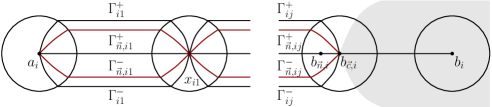
Figure 2. The arcs $\Gamma_{ij}^{\pm}$ and $\Gamma_{\vec{n},ij}^{\pm}$ in the case where there is at least one point in $E_{\mathsf{in}}$, $b_{\vec{n},i}<b_{\vec{c},i}<b_{i}$, and $b_{i}\in E_{\mathsf{out}}$.

Fix $\Gamma_{\vec{n},il}^{\pm}$ with endpoints $e_{1}<e_{2}$. There exists an index $k$ such that $x_{ij}\leq e_{1}$ for $j<k$ and $x_{ij}\geq e_{2}$ for $j\geq k$. Then it follows from (22) and (23) that the function $\rho_{i}$ holomorphically extends to $\Omega_{\vec{n},il}^{\pm}$ by

(55) $$\rho_{i}(z):=\rho_{\mathsf{r},i}(z)\prod_{j<k}\beta_{ij}\prod_{j<k}(z-x_{ij})^{\alpha_{ij}}\prod_{j\geq k}(x_{ij}-z)^{\alpha_{ij}},$$

where $(z-x_{ij})^{\alpha_{ij}}$ is holomorphic off $(-\infty,x_{ij}]$ and $(x_{ij}-z)^{\alpha_{ij}}$ is holomorphic off $[x_{ij},\infty)$. Using these extensions, set

(56) $$\boldsymbol{X}:=\boldsymbol{Y}\left\{\begin{array}[]{ll}\mathsf{T}_{i}\left(\begin{matrix}1&0\\ \mp 1/\rho_{i}&1\end{matrix}\right)&\mbox{in}\quad\Omega_{\vec{n},i}^{\pm},\vskip 6.0pt plus 2.0pt minus 2.0pt\\ \boldsymbol{I}&\text{otherwise},\end{array}\right.$$

where $\boldsymbol{Y}$ is a matrix-function that solves RHP-${\boldsymbol{Y}}$ (if it exists). It can be readily verified that ${\boldsymbol{X}}$ solves the following Riemann-Hilbert problem (RHP-${\boldsymbol{X}}$):

• ${\boldsymbol{X}}$ is analytic in $\mathbb{C}\setminus\bigcup_{i=1}^{p}\left([a_{i},b_{i}]\cup\Gamma_{\vec{n},i}^{+}\cup\Gamma_{\vec{n},i}^{-}\right)$ and $\displaystyle\lim_{z\to\infty}{\boldsymbol{X}}(z)z^{-\sigma(\vec{n})}={\boldsymbol{I}}$;

• ${\boldsymbol{X}}$ has continuous traces on $\bigcup_{i=1}^{p}\left((a_{i},b_{i})\cup\Gamma_{\vec{n},i}^{+}\cup\Gamma_{\vec{n},i}^{-}\right)$ that satisfy

  $${\boldsymbol{X}}_{+}={\boldsymbol{X}}_{-}\left\{\begin{array}[]{rl}\displaystyle\mathsf{T}_{i}\left(\begin{matrix}0&\rho_{i}\\ -1/\rho_{i}&0\end{matrix}\right)&\text{on}\quad\big{[}a_{\vec{c},i},b_{\vec{c},i}\big{]},\vskip 6.0pt plus 2.0pt minus 2.0pt\\ \displaystyle\mathsf{T}_{i}\left(\begin{matrix}1&\rho_{i}\\ 0&1\end{matrix}\right)&\text{on}\quad(a_{i},b_{i})\setminus\big{[}a_{\vec{c},i},b_{\vec{c},i}\big{]},\vskip 6.0pt plus 2.0pt minus 2.0pt\\ \displaystyle\mathsf{T}_{i}\left(\begin{matrix}1&0\\ 1/\rho_{i}&1\end{matrix}\right)&\text{on}\quad\Gamma_{\vec{n},i}^{+}\cup\Gamma_{\vec{n},i}^{-};\end{array}\right.$$

• $\boldsymbol{X}$ has the following behavior near $e\in E_{\vec{c}}\cup E_{\mathsf{in}}\cup E_{\mathsf{out}}$:

  • if $e\in E_{\mathsf{out}}$, then $\boldsymbol{X}$ satisfies RHP-${\boldsymbol{Y}}$(c) with $\boldsymbol{Y}$ replaced by $\boldsymbol{X}$;

  • if $e\in E_{\vec{c}}\setminus\{x_{ij}\}$, then all the entries of $\boldsymbol{X}$ are bounded at $e$;

  • if $e\in E_{\mathsf{in}}$ or $e\in E_{\vec{c}}\cap\{x_{ij}\}$, then $\boldsymbol{X}$ satisfies RHP-${\boldsymbol{Y}}$(c) with $\boldsymbol{Y}$ replaced by $\boldsymbol{X}$ outside of $\overline{\Omega_{\vec{n},i}^{+}\cup\Omega_{\vec{n},i}^{-}}$ while inside it behaves exactly as in RHP-${\boldsymbol{Y}}$(c) when $\alpha_{ij}<0$, the entries of the first and $(i+1)$-st column behave like $\mathcal{O}(\psi_{0}(z-x_{ij}))$ and the rest of the entries are bounded when $\alpha_{ij}=0$, and the entries of the first column behave like $\mathcal{O}(\psi_{-\alpha_{ij}}(z-x_{ij}))$ and the rest of the entries are bounded when $\alpha_{ij}>0$.

Due to the block structure of the jumps in RHP-${\boldsymbol{Y}}$(b), [5, Lemma 17] can be carried over word for word to the present case to prove:

Lemma 8.

RHP-${\boldsymbol{X}}$ is solvable if and only if RHP-${\boldsymbol{Y}}$ is solvable. When solutions of RHP-${\boldsymbol{X}}$ and RHP-${\boldsymbol{Y}}$ exist, they are unique and connected by (56).

8.2   Auxiliary Parametrices

To solve RHP-${\boldsymbol{X}}$, we construct parametrices that asymptotically describe the behavior of $\boldsymbol{X}$ away from and around each point in $E_{\mathsf{in}}\cup E_{\mathsf{out}}\cup E_{\vec{c}}$. To this end, we construct a matrix-valued function $\boldsymbol{N}$ that solves the following Riemann-Hilbert problem (RHP-${\boldsymbol{N}}$):

• ${\boldsymbol{N}}$ is analytic in $\mathbb{C}\setminus\bigcup_{i=1}^{p}\big{[}a_{\vec{n},i},b_{\vec{n},i}\big{]}$ and $\displaystyle\lim_{z\to\infty}{\boldsymbol{N}}(z)z^{-\sigma(\vec{n})}={\boldsymbol{I}}$;

• ${\boldsymbol{N}}$ has continuous traces on $\big{(}a_{\vec{n},i},b_{\vec{n},i}\big{)}$ that satisfy $\boldsymbol{N}_{+}=\boldsymbol{N}_{-}\displaystyle\mathsf{T}_{i}\left(\begin{matrix}0&\rho_{i}\\ -1/\rho_{i}&0\end{matrix}\right)$.

Let $\Phi_{\vec{n}}$ be the functions from Proposition 1 while $S_{\vec{n}}$ and $\Upsilon_{\vec{n},i}$, $i\in\{1,\ldots,p\},$ be the functions introduced in Section 7. Set

(57) $$\boldsymbol{N}:=\boldsymbol{CMD},$$

where $\boldsymbol{D}:=\mathsf{diag}\left(\Phi_{\vec{n}}^{(0)},\ldots,\Phi_{\vec{n}}^{(p)}\right)$, $\boldsymbol{C}:=\mathsf{diag}\left(C_{\vec{n},0},\ldots,C_{\vec{n},p}\right)$ with the constant $C_{\vec{n},k}$ defined by

(58) $$\left\{\begin{array}[]{lcl}\displaystyle\lim_{z\to\infty}C_{\vec{n},0}\big{(}S_{\vec{n}}\Phi_{\vec{n}}\big{)}^{(0)}(z)z^{-|\>\vec{n}\>|}&=&1\vskip 6.0pt plus 2.0pt minus 2.0pt\\ \displaystyle\lim_{z\to\infty}C_{\vec{n},i}\big{(}S_{\vec{n}}\Phi_{\vec{n}}\big{)}^{(i)}(z)z^{n_{i}}&=&1,\quad i\in\{1,\ldots,p\},\end{array}\right.$$

and the matrix $\boldsymbol{M}$ is given by

(59) $$\boldsymbol{M}:=\left(\begin{array}[]{cccc}S_{\vec{n}}^{(0)}&S_{\vec{n}}^{(1)}/w_{\vec{n},1}&\cdots&S_{\vec{n}}^{(p)}/w_{\vec{n},p}\vskip 6.0pt plus 2.0pt minus 2.0pt\\ \big{(}S_{\vec{n}}\Upsilon_{\vec{n},1}\big{)}^{(0)}&\big{(}S_{\vec{n}}\Upsilon_{\vec{n},1}\big{)}^{(1)}/w_{\vec{n},1}&\cdots&\big{(}S_{\vec{n}}\Upsilon_{\vec{n},1}\big{)}^{(p)}/w_{\vec{n},p}\vskip 3.0pt plus 1.0pt minus 1.0pt\\ \vdots&\vdots&\ddots&\vdots\\ \big{(}S_{\vec{n}}\Upsilon_{\vec{n},p}\big{)}^{(0)}&\big{(}S_{\vec{n}}\Upsilon_{\vec{n},p}\big{)}^{(1)}/w_{\vec{n},1}&\cdots&\big{(}S_{\vec{n}}\Upsilon_{\vec{n},p}\big{)}^{(p)}/w_{\vec{n},p}\end{array}\right).$$

Then (57) solves RHP-${\boldsymbol{N}}$. Indeed, RHP-${\boldsymbol{N}}$(a) follows immediately from the analyticity properties of $S_{\vec{n}}$, $\Upsilon_{\vec{n},i}$, and $\Phi_{\vec{n}}$ as well as from (58). Observe that the multiplication by

$$\mathsf{T}_{i}\left(\begin{matrix}0&\rho_{i}\\ -1/\rho_{i}&0\end{matrix}\right)$$

on the right replaces the first column by the $(i+1)$-st one multiplied by $\rho_{i}$, while $(i+1)$-st column is replaced by the first one multiplied by $-1/\rho_{i}$. Hence, RHP-${\boldsymbol{N}}$(b) follows from the analog of (25) for $S_{\vec{n}}$ and the fact that any rational function $\Psi$ on $\boldsymbol{\mathfrak{R}}_{\vec{n}}$ satisfies $\Psi_{\pm}^{(0)}=\Psi_{\mp}^{(i)}$ on $\big{(}a_{\vec{n},i},b_{\vec{n},i}\big{)}$.

Since the jump matrices in RHP-${\boldsymbol{N}}$(b) have determinant 1, $\mathsf{det}(\boldsymbol{N})$ is a holomorphic function in $\overline{\mathbb{C}}\setminus\bigcup_{i}\big{\{}a_{\vec{n},i},b_{\vec{n},i}\big{\}}$ and $\mathsf{det}(\boldsymbol{N})(\infty)=1$. Moreover, it follows from the analogs of (26) and (27) for $S_{\vec{n}}$ that each entry of the first column of $\boldsymbol{N}$ behaves like

$$\mathcal{O}\left(|z-e|^{-(2\alpha+1)/4}\right)\quad\text{and}\quad\mathcal{O}\left(|z-x_{ij}|^{-(\alpha_{ij}\mp\mathsf{arg}(\beta_{ij})/\pi)/2}\right)$$

for $e\in\big{\{}a_{\vec{n},i},b_{\vec{n},i}\big{\}}$ ($\alpha=\alpha_{ij}$ if $e=x_{ij}$ and $\alpha=0$ otherwise) and for $x_{ij}\in\big{(}a_{\vec{n},i},b_{\vec{n},i}\big{)}$ ($\pm\mathsf{Im}(z)>0$), respectively, the entries of the $(i+1)$-st column behave like

$$\mathcal{O}\left(|z-e|^{(2\alpha-1)/4}\right)\quad\text{and}\quad\mathcal{O}\left(|z-x_{ij}|^{(\alpha_{ij}\mp\mathsf{arg}(\beta_{ij})/\pi)/2}\right)$$

there, and the rest of the entries are bounded. Thus, the determinant has at most square root singularities at these points and therefore is a bounded entire function. That is, $\mathsf{det}(\boldsymbol{N})\equiv 1$ as follows from the normalization at infinity.

Further, for each $e\in E_{\mathsf{in}}\cup E_{\mathsf{out}}\cup E_{\vec{c}}$, we want to solve RHP-${\boldsymbol{X}}$ locally in $U_{e}$. That is, we are seeking a solution of the following RHP-${\boldsymbol{P}}_{e}$:

• $\boldsymbol{P}_{e}$ satisfies RHP-${\boldsymbol{X}}$(a,b,c) within $U_{e}$;

• $\boldsymbol{P}_{e}=\boldsymbol{M}\left(\boldsymbol{I}+\boldsymbol{\mathcal{O}}(\varepsilon_{e,\vec{n}})\right)\boldsymbol{D}$ uniformly on $\partial U_{e}\setminus\left([a_{i},b_{i}]\cup\bigcup_{i=1}^{p}\Gamma_{\vec{n},i}^{+}\cup\Gamma_{\vec{n},i}^{-}\right)$, where $0<\varepsilon_{e,\vec{n}}\to 0$ as $|\>\vec{n}\>|\to\infty$.

Since the construction of $\boldsymbol{P}_{e}$ solving RHP-${\boldsymbol{P}}_{e}$  is rather lengthy, it is carried out separately in Section 9 further below.

8.3   Final R-H Problem

Denote by $\Omega_{\vec{n},ij}$ the domain delimited by $\Gamma_{\vec{n},ij}^{+}$ and $\Gamma_{\vec{n},ij}^{-}$ (in particular, $\Omega_{\vec{n},ij}^{\pm}\subset\Omega_{\vec{n},ij}$). Set $\Omega_{\vec{n}}:=\bigcup_{ij}\Omega_{\vec{n},ij}$ and $U:=\bigcup_{e\in E_{\mathsf{in}}\cup E_{\mathsf{out}}\cup E_{\vec{c}}}U_{e}$. Define

$$\Sigma_{\vec{n}}:=\partial U\cup\left[\bigcup_{i=1}^{p}\left(\Gamma_{\vec{n},i}^{+}\cup\Gamma_{\vec{n},i}^{-}\right)\setminus U\right]\cup\left[\bigcup_{i=1}^{p}[a_{i},b_{i}]\setminus\big{(}U\cup\Omega_{\vec{n}}\big{)}\right].$$

Moreover, we define $\Sigma$ by replacing $\Gamma_{\vec{n},i}^{\pm}$ with $\Gamma_{i}^{\pm}$ in the definition of $\Sigma_{\vec{n}}$ see Figure 3.

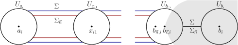
Figure 3. Contours $\Sigma$ (black and blue lines) and $\Sigma_{\vec{n}}$ (black and red lines).

Given matrices $\boldsymbol{N}$ and $\boldsymbol{P}_{e}$, $e\in E_{\mathsf{in}}\cup E_{\mathsf{out}}\cup E_{\vec{c}}$, from the previous section, consider the following Riemann-Hilbert Problem (RHP-${\boldsymbol{Z}}$):

• $\boldsymbol{Z}$ is a holomorphic matrix function in $\overline{\mathbb{C}}\setminus\Sigma_{\vec{n}}$ and $\boldsymbol{Z}(\infty)=\boldsymbol{I}$;

• $\boldsymbol{Z}$ has continuous traces on $\Sigma_{\vec{n}}$ that satisfy

  $$\boldsymbol{Z}_{+}=\boldsymbol{Z}_{-}\left\{\begin{array}[]{ll}\boldsymbol{MD}\mathsf{T}_{i}\left(\begin{matrix}1&0\\ 1/\rho_{i}&1\end{matrix}\right)(\boldsymbol{MD})^{-1}&\text{on}\quad\left(\Gamma_{\vec{n},i}^{+}\cup\Gamma_{\vec{n},i}^{-}\right)\setminus\overline{U},\vskip 6.0pt plus 2.0pt minus 2.0pt\\ \boldsymbol{MD}\mathsf{T}_{i}\left(\begin{matrix}1&\rho_{i}\\ 0&1\end{matrix}\right)(\boldsymbol{MD})^{-1}&\text{on}\quad[a_{i},b_{i}]\setminus\big{(}\overline{U\cup\Omega_{\vec{n}}}\big{)}\vskip 6.0pt plus 2.0pt minus 2.0pt\\ \boldsymbol{P}_{e}(\boldsymbol{MD})^{-1}&\text{on}\quad\partial U_{e}.\end{array}\right.$$

Then the following lemma takes place.

Lemma 9.

The solution of RHP-${\boldsymbol{Z}}$ exists for all $|\>\vec{n}\>|$ large enough and satisfies

(60) $$\boldsymbol{Z}=\boldsymbol{I}+\mathcal{O}\big{(}\varepsilon_{\vec{n}}\big{)}$$

uniformly in $\overline{\mathbb{C}}$, where $\varepsilon_{\vec{n}}=\min_{e}\varepsilon_{e,\vec{n}}$.

Proof.

Analyticity of $\rho_{i}$ yields that $\boldsymbol{Z}$ can be analytically continued to be holomorphic outside of $\Sigma$. To do that one simply needs to multiply $\boldsymbol{Z}$ by the first jump matrix in RHP-${\boldsymbol{Z}}$(b) or its inverse (the jump matrices have determinate 1 and therefore are invertible). We shall show that the jump matrices are locally uniformly geometrically small in $D_{i}^{+}$. This would imply that the new problem is solvable if and only if the initial problem is solvable and the bound (60) remains valid regardless the contour. Hence, in what follows we shall consider RHP-${\boldsymbol{Z}}$  on $\Sigma$ rather than on $\Sigma_{\vec{n}}$.

It was shown in Section 8.2 that $\mathsf{det}(\boldsymbol{N})\equiv 1$. Moreover, it follows from (18) that $\mathsf{det}(\boldsymbol{D})\equiv 1$ while the equality $\prod_{k=0}^{p}S^{(k)}_{\vec{n}}\equiv 1$ and (58) imply that $\mathsf{det}(\boldsymbol{C})\equiv 1$. Hence, $\mathsf{det}(\boldsymbol{M})\equiv 1$ and it follows from RHP-${\boldsymbol{P}}_{e}$(d), (51), and (50) that

$$\boldsymbol{P}_{e}(\boldsymbol{MD})^{-1}=\boldsymbol{I}+\boldsymbol{M}\mathcal{O}\big{(}\varepsilon_{e,\vec{n}}\big{)}\boldsymbol{M}^{-1}=\boldsymbol{I}+\mathcal{O}(\varepsilon_{e,\vec{n}})$$

holds uniformly on each $\partial U_{e}$. On the other hand, it holds on $\Gamma_{i}^{\pm}\setminus\overline{U}$ that

$$\boldsymbol{MD}\mathsf{T_{i}}\left(\begin{matrix}1&0\\ 1/\rho_{i}&1\end{matrix}\right)(\boldsymbol{MD})^{-1}=\boldsymbol{I}+\frac{1}{\rho_{i}}\frac{\Phi_{\vec{n}}^{(i)}}{\Phi_{\vec{n}}^{(0)}}\boldsymbol{M}\boldsymbol{E}_{i+1,1}\boldsymbol{M}^{-1}=\boldsymbol{I}+\mathcal{O}\left(C_{i}^{-|\>\vec{n}\>|}\right)$$

for some constant $C_{i}>1$ by (15), (19), and Proposition 1. Analogously, we get that

$$\boldsymbol{MD}\mathsf{T_{i}}\left(\begin{matrix}1&\rho_{i}\\ 0&1\end{matrix}\right)(\boldsymbol{MD})^{-1}=\boldsymbol{I}+\rho_{i}\frac{\Phi_{\vec{n}}^{(0)}}{\Phi_{\vec{n}}^{(i)}}\boldsymbol{M}\boldsymbol{E}_{1,i+1}\boldsymbol{M}^{-1}=\boldsymbol{I}+\mathcal{O}\left(\widetilde{C}_{i}^{-|\>\vec{n}\>|}\right)$$

on $[a_{i},b_{i}]\setminus\big{(}\overline{U\cup\Omega_{\vec{n}}}\big{)}$ for some $\widetilde{C}_{i}>1$ by (19) and (14). That is, all the jump matrices for $\boldsymbol{Z}$ asymptotically behave like $\boldsymbol{I}+\mathcal{O}\big{(}\varepsilon_{\vec{n}}\big{)}$ (as will be clear in Section 9, the decay of $\varepsilon_{\vec{n}}$ is of power type and not exponential). The conclusion of the lemma follows from the same argument as in [7, Corollary 7.108]. ∎

8.4   Proof of Theorem 5

Let $\boldsymbol{Z}$ be the solution of RHP-${\boldsymbol{Z}}$ granted by Lemma 9, $\boldsymbol{P}_{e}$ be solutions of RHP-${\boldsymbol{P}}_{e}$, and $\boldsymbol{N}=\boldsymbol{CMD}$ be the matrix constructed in (57). Then it can be easily checked that

(61) $$\boldsymbol{X}=\boldsymbol{C}\boldsymbol{Z}\left\{\begin{array}[]{rll}\boldsymbol{M}\boldsymbol{D}&\text{in}&\mathbb{C}\setminus\big{(}\overline{U}\cup\bigcup\big{[}a_{\vec{c},i}b_{\vec{c},i}\big{]}\big{)},\vskip 6.0pt plus 2.0pt minus 2.0pt\\ \boldsymbol{P}_{e}&\text{in}&U_{e},\quad e\in E_{\mathsf{out}}\cup E_{\mathsf{in}}\cup E_{\vec{c}},\end{array}\right.$$

solves RHP-${\boldsymbol{X}}$ for all $|\>\vec{n}\>|$ large enough. Given a closed set $K$ in $\overline{\mathbb{C}}\setminus\bigcup_{i=1}^{p}[a_{i},b_{i}]$, we can always shrink the lens so that $K\subset\mathbb{C}\setminus\big{(}\overline{U\cup\Omega_{\vec{n}}}\big{)}$. In this case $\boldsymbol{Y}=\boldsymbol{X}$ on $K$ by Lemma 8. Write the first row of $\boldsymbol{Z}$ as $\left(1+\upsilon_{\vec{n},0},\upsilon_{\vec{n},1},\ldots,\upsilon_{\vec{n},p}\right)$. Then $(1,j+1)$-st entry of $\boldsymbol{ZM}$ is equal to

$$\left(1+\upsilon_{\vec{n},0}+\sum_{i=1}^{p}\upsilon_{\vec{n},i}\Upsilon_{\vec{n},i}^{(j)}\right)S_{\vec{n}}^{(j)}/w_{\vec{n},j}=\big{(}1+\mathcal{O}(\varepsilon_{\vec{n}})\big{)}S_{\vec{n}}^{(j)}/w_{\vec{n},j}$$

by Lemma 9 and (50), where $w_{\vec{n},0}\equiv 1$. Therefore, it follows from Proposition 6 that

$$\left\{\begin{array}[]{lll}Q_{\vec{n}}&=&C_{\vec{n},0}\big{[}1+\mathcal{O}(\varepsilon_{\vec{n}})\big{]}\big{(}S_{\vec{n}}\Phi_{\vec{n}}\big{)}^{(0)}\vskip 6.0pt plus 2.0pt minus 2.0pt\\ R_{\vec{n}}^{(j)}&=&C_{\vec{n},0}\big{[}1+\mathcal{O}(\varepsilon_{\vec{n}})\big{]}\big{(}S_{\vec{n}}\Phi_{\vec{n}}\big{)}^{(j)}/w_{\vec{n},j}.\end{array}\right.$$

Theorem 5 now follows from (51), since $C_{\vec{n},0}=(1+o(1))C_{\vec{n}}$ again by (51) and $w_{\vec{n},j}\to w_{j}$ uniformly on $K$.

9   Local Riemann-Hilbert Analysis

The goal of this section is to construct solutions to RHP-${\boldsymbol{P}}_{e}$.

9.1   Local Parametrices around Points in $E_{\mathsf{out}}$

Let $e\in E_{\mathsf{out}}$, see (52). A solution of RHP-${\boldsymbol{P}}_{e}$ is given by

(62) $$\boldsymbol{P}_{e}:=\boldsymbol{M}\mathsf{T}_{i}\left(\begin{matrix}1&\mathcal{C}_{i}\Phi_{\vec{n}}^{(0)}/\Phi_{\vec{n}}^{(i)}\\ 0&1\end{matrix}\right)\boldsymbol{D},$$

where $\mathcal{C}_{i}(z):=\frac{1}{2\pi\mathrm{i}}\int_{[a_{i},b_{i}]}\frac{\rho_{i}(x)}{x-z}\mathrm{d}x$. Indeed, since the matrices $\boldsymbol{M}$ and $\boldsymbol{D}$ are holomorphic in $U_{e}$, and $\mathcal{C}_{i}$ has a jump only across $(a_{i},b_{i})\cap U_{e}$, the matrix above satisfies RHP-${\boldsymbol{P}}_{e}$(a). As $\big{(}\mathcal{C}_{i}^{+}-\mathcal{C}_{i}^{-}\big{)}(x)=\rho_{i}(x)$ for $x\in(a_{i},b_{i})\setminus\{x_{ij}\}$, RHP-${\boldsymbol{P}}_{e}$(b) follows. RHP-${\boldsymbol{P}}_{e}$(c) is a consequence of the fact that $\big{|}\mathcal{C}_{i}(z)(z-x_{ij})^{-\alpha_{ij}}\big{|}$ is bounded in the vicinity of $x_{ij}$ for $\alpha_{ij}<0$, [13, Sec. 8.3]. Finally, RHP-${\boldsymbol{P}}_{e}$(d) is easily deduced from the inclusion $\overline{U}_{e}\subset D_{i}^{-}$, (19) and (14).

9.2   Local Parametrices around Points in $E_{\mathsf{in}}$

The construction below is known [30, 21, 22, 8].

9.2.1   Conformal Maps

Since $h$ is a rational function on $\boldsymbol{\mathfrak{R}}$, it holds that $h^{(0)}_{\pm}=h^{(i)}_{\mp}$ on $\big{(}a_{\vec{c},i},b_{\vec{c},i}\big{)}\cap U_{e}$. Then

(63) $$\zeta_{e}(z):=\mathsf{sgn}\big{(}\mathsf{Im}(z)\big{)}\mathrm{i}\int_{e}^{z}\left(h^{(0)}-h^{(i)}\right)(x)\mathrm{d}x,\quad\mathsf{Im}(z)\neq 0,$$

extends to a conformal function in $U_{e}$ vanishing at $e$. Define $\zeta_{\vec{n},e}$ exactly as in (63) with $h$ replaced by $h_{\vec{n}}$. Then it holds that

(64) $$\zeta_{\vec{n},e}(z)=\frac{\mathsf{sgn}\big{(}\mathsf{Im}(z)\big{)}\mathrm{i}}{|\>\vec{n}\>|}\log\left(\Phi_{\vec{n}}^{(0)}(z)/\Phi_{\vec{n}}^{(i)}(z)\right),\quad\mathsf{Im}(z)\neq 0,$$

by (21). It follows from (19) and (14) that $\zeta_{\vec{n},e}$ is real on $\big{(}a_{\vec{c},i},b_{\vec{c},i}\big{)}\cap U_{e}$. Moreover, since $U_{e}\setminus\big{(}a_{\vec{c},i},b_{\vec{c},i}\big{)}\subset D_{i}^{+}$, $\zeta_{\vec{n},e}$ maps upper half-plane into the upper half-plane. In particular, $\zeta_{\vec{n},e}(x)>0$ for $x\in\big{(}e,b_{\vec{c},i}\big{)}\cap U_{e}$. Observe also that

(65) $$\zeta_{\vec{n},e}\to\zeta_{e}$$

holds uniformly on $\overline{U}_{e}$ by (19) since (19) is the statement about convergence of the imaginary parts of $\zeta_{\vec{n},e}$ to the imaginary part of $\zeta_{e}$.

9.2.2   Matrix $\boldsymbol{P}_{e}$

It follows from the way we extended $\rho_{i}$ into $\Omega_{\vec{n},i}^{\pm}$ that we can write

(66) $$\rho_{i}(z)=\rho_{\mathsf{r},e}(z)\left\{\begin{array}[]{rl}(e-z)^{\alpha},&\mathsf{Re}(z)<e,\vskip 3.0pt plus 1.0pt minus 1.0pt\\ \beta(z-e)^{\alpha},&\mathsf{Re}(z)>e,\end{array}\right.$$

where $\rho_{\mathsf{r},e}(x)$ is a holomorphic and non-vanishing function in $U_{e}$. Define $r_{e}$ by

$$r_{e}(z):=\sqrt{\rho_{\mathsf{r},e}(z)}(z-e)^{\alpha/2},$$

where the square root is principal. Then $r_{e}$ is a holomorphic and non-vanishing function in $U_{e}\setminus\{x:x<e\}$ that satisfies

(67) $$\left\{\begin{array}[]{ll}r_{e+}(x)r_{e-}(x)=\rho_{i}(x),&x\in\{x:x<e\}\cap U_{e},\vskip 6.0pt plus 2.0pt minus 2.0pt\\ r_{e}^{2}(z)=\rho_{i}(z)e^{\pm\pi\mathrm{i}\alpha},&z\in\Gamma_{\vec{n},ij}^{\pm}\cap U_{e},\vskip 6.0pt plus 2.0pt minus 2.0pt\\ r_{e}^{2}(x)=\beta^{-1}\rho_{i}(x),&\left(\Gamma_{\vec{n},ij+1}^{+}\cup\Gamma_{\vec{n},ij+1}^{-}\cup\{x:x>e\}\right)\cap U_{e}.\end{array}\right.$$

It is a straightforward computation using (67) and (64) to verify that RHP-${\boldsymbol{P}}_{e}$ is solved by

$$\boldsymbol{P}_{e}:=\boldsymbol{E}_{e}\mathsf{T}_{i}\left(\boldsymbol{\Phi}_{\alpha,\beta}\left(|\>\vec{n}\>|\zeta_{\vec{n},e}\right)r_{e}^{-\sigma_{3}}\left(\Phi^{(0)}_{\vec{n}}/\Phi^{(i)}_{\vec{n}}\right)^{-\sigma_{3}/2}\right)\boldsymbol{D},$$

where $\boldsymbol{\Phi}_{\alpha,\beta}$ is the solution of RHP-${\boldsymbol{\Phi}_{\alpha,\beta}}$ and the holomorphic prefactor $\boldsymbol{E}_{e}$ chosen below to fulfill RHP-${\boldsymbol{P}}_{e}$(d).

9.2.3   Holomorphic Prefactor $\boldsymbol{E}_{e}$

It follows from the properties of the branch of $\big{(}\mathrm{i}\zeta\big{)}^{\log\beta\sigma_{3}/2\pi\mathrm{i}}$ that

(68) $$\big{(}\mathrm{i}\zeta\big{)}_{+}^{\log\beta\sigma_{3}/2\pi\mathrm{i}}\boldsymbol{B}_{+}=\big{(}\mathrm{i}\zeta\big{)}_{-}^{\log\beta\sigma_{3}/2\pi\mathrm{i}}\boldsymbol{B}_{-}\left\{\begin{array}[]{lll}\left(\begin{matrix}0&1\\ -1&0\end{matrix}\right)&\text{on}&(-\infty,0),\vskip 6.0pt plus 2.0pt minus 2.0pt\\ \left(\begin{matrix}0&\beta\\ -1/\beta&0\end{matrix}\right)&\text{on}&(0,\infty),\end{array}\right.$$

and it is holomorphic in $\mathbb{C}\setminus(-\infty,\infty)$. Therefore, it follows from RHP-${\boldsymbol{N}}$(b) that

$$\boldsymbol{E}_{e}:=\boldsymbol{M}\mathsf{T}_{i}\left(\big{(}\mathrm{i}|\>\vec{n}\>|\zeta_{\vec{n},e}\big{)}^{\log\beta\sigma_{3}/2\pi\mathrm{i}}\boldsymbol{B}_{\pm}r_{e}^{-\sigma_{3}}\right)^{-1},\quad\pm\mathsf{Im}(z)>0,$$

is holomorphic in $U_{e}\setminus\{e\}$. Since $|r_{e}(z)|\sim|z-e|^{\alpha/2}$ and $\big{|}\zeta^{\log\beta/2\pi\mathrm{i}}\big{|}\sim|\zeta|^{\mathsf{arg}(\beta)/2\pi}$, $\boldsymbol{E}_{e}$ is in fact holomorphic in $U_{e}$ as claimed. Clearly, in this case it holds that $\varepsilon_{\vec{n},e}=|\>\vec{n}\>|^{|\mathsf{arg}(\beta)|/\pi-1}$.

9.3   Hard Edge

In this section we assume that $e\in E_{\vec{c}}$ and $e\not\in\partial D_{i}^{-}$.

9.3.1   Conformal Maps

It follows from Proposition 3 that $b_{\vec{c},i}=b_{\vec{n},i}=b_{i}$ or $a_{\vec{c},i}=a_{\vec{n},i}=a_{i}$ for all $|\>\vec{n}\>|$ large in this case. Define

(69) $$\zeta_{e}(z):=\left(\frac{1}{4}\int_{e}^{z}\left(h^{(0)}-h^{(i)}\right)(x)\mathrm{d}x\right)^{2},\quad z\in U_{e}.$$

Since $h_{\pm}^{(0)}=h_{\mp}^{(i)}$ on $(a_{i},b_{i})\cap U_{e}$, $\zeta_{e}$ is holomorphic in $U_{e}$. Moreover, since $h$ has a pole at $\boldsymbol{e}$ (the corresponding branch point of $\boldsymbol{\mathfrak{R}}$), $\zeta_{e}$ has a simple zero at $e$. Thus, we can choose $U_{e}$ small enough so that $\zeta_{e}$ is conformal in $\overline{U}_{e}$.

Define $\zeta_{\vec{n},e}$ as in (69) with $h$ replaced by $h_{\vec{n}}$. The functions $\zeta_{\vec{n},e}$ form a family of holomorphic functions in $U_{e}$, all having a simple zero at $e$. Moreover, (21) yields that

(70) $$\zeta_{\vec{n},e}(z)=\left(\frac{1}{4|\>\vec{n}\>|}\log\left(\Phi_{\vec{n}}^{(0)}/\Phi_{\vec{n}}^{(i)}\right)\right)^{2},\quad z\in U_{e},$$

which, together with (15) and (19), implies that $\zeta_{\vec{n},e}(x)$ is positive for $x\in\big{(}\mathbb{R}\setminus[a_{i},b_{i}])\cap U_{e}$ and is negative $x\in(a_{i},b_{i})\cap U_{e}$ (this also can be seen from (37) and (38)).

Considering $h_{\vec{n}}$ and $h$ as defined on the same doubly circular neighborhood of $\boldsymbol{e}$ and recalling that their ratio converges to 1 on its boundary, we see that it converges to 1 uniformly throughout the neighborhood. The latter implies that (65) holds uniformly on $\overline{U}_{e}$. In particular, the functions $\zeta_{\vec{n},e}$ are conformal in $\overline{U}_{e}$ for all $\vec{n}$ large.

9.3.2   Matrix $\boldsymbol{P}_{e}$

In this case we can write

(71) $$\rho_{i}(z)=\rho_{\mathsf{r},e}(z)\left\{\begin{array}[]{ll}(e-z)^{\alpha},&e=b_{i},\vskip 3.0pt plus 1.0pt minus 1.0pt\\ (z-e)^{\alpha},&e=a_{i},\end{array}\right.$$

where $\rho_{\mathsf{r},e}$ is non-vanishing and holomorphic in $U_{e}$, $\alpha>-1$, and the $\alpha$-roots are principal. Set

(72) $$r_{e}(z):=\sqrt{\rho_{\mathsf{r},e}(z)}\left\{\begin{array}[]{ll}(z-e)^{\alpha/2},&e=b_{i},\vskip 3.0pt plus 1.0pt minus 1.0pt\\ (e-z)^{\alpha/2},&e=a_{i},\end{array}\right.$$

where the branches are again principal. Then $r_{e}$ is a holomorphic and non-vanishing function in $U_{e}\setminus[a_{i},b_{i}]$ and satisfies

(73) $$\left\{\begin{array}[]{ll}r_{e+}(x)r_{e-}(x)=\rho_{i}(x),&x\in(a_{i},b_{i}),\vskip 6.0pt plus 2.0pt minus 2.0pt\\ r_{e}^{2}(z)=\rho_{i}(z)e^{\pm\pi\mathrm{i}\alpha},&z\in\Gamma_{\vec{n},i}^{\pm}\cap U_{e}.\end{array}\right.$$

Then (70) and (73) imply that RHP-${\boldsymbol{P}}_{e}$ is solved by

(74) $$\boldsymbol{P}_{e}:=\boldsymbol{E}_{e}\mathsf{T}_{i}\left(\boldsymbol{\Psi}_{e}\left(|\>\vec{n}\>|^{2}\zeta_{\vec{n},e}\right)r_{e}^{-\sigma_{3}}\left(\Phi^{(0)}_{\vec{n}}/\Phi^{(i)}_{\vec{n}}\right)^{-\sigma_{3}/2}\right)\boldsymbol{D},$$

where $\boldsymbol{\Psi}_{e}:=\boldsymbol{\Psi}_{\alpha}$ when $e=b_{i}$ and $\boldsymbol{\Psi}_{e}:=\sigma_{3}\boldsymbol{\Psi}_{\alpha}\sigma_{3}$ when $e=a_{i}$, and $\boldsymbol{\Psi}_{\alpha}$ solves RHP-${\boldsymbol{\Psi}_{\alpha}}$, while $\boldsymbol{E}_{e}$ is a holomorphic prefactor chosen so that RHP-${\boldsymbol{P}}_{e}$(d) is fulfilled.

9.3.3   Holomorphic Prefactor $\boldsymbol{E}_{e}$

As $\zeta_{+}^{1/4}=\mathrm{i}\zeta^{1/4}_{-}$, it can be easily checked that

$$\frac{\zeta_{+}^{-\sigma_{3}/4}}{\sqrt{2}}\left(\begin{matrix}1&\pm\mathrm{i}\\ \pm\mathrm{i}&1\end{matrix}\right)=\frac{\zeta_{-}^{-\sigma_{3}/4}}{\sqrt{2}}\left(\begin{matrix}1&\pm\mathrm{i}\\ \pm\mathrm{i}&1\end{matrix}\right)\left(\begin{matrix}0&\pm 1\\ \mp 1&0\end{matrix}\right)$$

on $(-\infty,0)$. Then RHP-${\boldsymbol{N}}$(b) implies that

(75) $$\boldsymbol{E}_{e}:=\boldsymbol{M}\mathsf{T}_{i}\left(\frac{(|\>\vec{n}\>|^{2}\zeta_{\vec{n},e}\big{)}^{-\sigma_{3}/4}}{\sqrt{2}}\left(\begin{matrix}1&\pm\mathrm{i}\\ \pm\mathrm{i}&1\end{matrix}\right)r_{e}^{-\sigma_{3}}\right)^{-1}$$

is holomorphic around in $U_{e}\setminus\{e\}$, where the sign $+$ is used around $e=b_{i}$ while the sign $-$ is used around $e=a_{i}$. Since $|r_{e}(z)|\sim|z-e|^{\alpha/2}$, $\boldsymbol{E}_{e}$ is in fact holomorphic in $U_{e}$ as desired. Clearly, $\varepsilon_{\vec{n},e}=|\>\vec{n}\>|^{-1}$ in this case.

9.4   Soft-Type Edge I

Below, we assume that $e\in E_{\vec{c}}$ and $b_{\vec{n},i}\in\partial D_{\vec{n},i}^{-}$ or $a_{\vec{n},i}\in\partial D_{\vec{n},i}^{-}$.

9.4.1   Conformal Maps

By the condition of this section, it holds that $e\in\partial D_{i}^{-}$. Define

(76) $$\zeta_{e}(z):=\left(-\frac{3}{4}\int_{e}^{z}\left(h^{(0)}-h^{(i)}\right)(x)\mathrm{d}x\right)^{2/3},\quad z\in U_{e}.$$

Further, define $\zeta_{\vec{n},e}$ exactly as $\zeta_{e}$ only with $h$ replaced by $h_{\vec{n}}$ and $e$ replaced by $b_{\vec{n},i}$ if $e=b_{\vec{c},i}$ and by $a_{\vec{n},i}$ if $e=a_{\vec{c},i}$. It follows from (21) that

(77) $$\zeta_{\vec{n},e}(z)=\left(-\frac{3}{4|\>\vec{n}\>|}\log\left(\Phi_{\vec{n}}^{(0)}(z)/\Phi_{\vec{n}}^{(i)}(z)\right)\right)^{2/3},\quad z\in U_{e}.$$

Analysis in (37) and (39) yields that these functions are conformal in $\overline{U}_{e}$ (make the radius smaller if necessary), are positive on $\big{(}\mathbb{R}\setminus\big{[}a_{\vec{n},i},b_{\vec{n},i}\big{]})\cap U_{e}$ and negative on $\big{(}a_{\vec{n},i},b_{\vec{n},i})\cap U_{e}$. Moreover, (65) holds as well.

9.4.2   Matrix $\boldsymbol{P}_{e}$

If $e=x_{ij}$ for some $j\in\{1,\ldots,J_{i}-1\}$, set $\alpha:=\alpha_{ij}$ and $\beta:=\beta_{ij}$ when $e=b_{\vec{c},i}$ or $\beta:=1/\beta_{ij}$ when $e=a_{\vec{c},i}$, see (23); if $e\not\in\{x_{ij}\}_{j=1}^{J_{i}-1}$ and $e\in(a_{i},b_{i})$, set $\alpha=0$ and $\beta=1$; if $e=a_{i}$, set $\alpha=\alpha_{i0}$ and $\beta=0$; if $e=b_{i}$, set $\alpha=\alpha_{iJ_{i}}$ and $\beta=0$. It follows from the way we extended $\rho_{i}$ into $\Omega_{\vec{n},i}^{\pm}$ that

(78) $$\rho_{i}(z)=\rho_{\mathsf{r},e}(z)\left\{\begin{array}[]{ll}(e-z)^{\alpha},&e=b_{\vec{c},i},\vskip 3.0pt plus 1.0pt minus 1.0pt\\ (z-e)^{\alpha},&e=a_{\vec{c},i},\end{array}\right.$$

for $\mathsf{Re}(z)\in\big{(}a_{\vec{c},i},b_{\vec{c},i}\big{)}$ and

(79) $$\rho_{i}(z)=\beta\rho_{\mathsf{r},e}(z)\left\{\begin{array}[]{ll}(z-e)^{\alpha},&e=b_{\vec{c},i},\vskip 3.0pt plus 1.0pt minus 1.0pt\\ (e-z)^{\alpha},&e=a_{\vec{c},i},\end{array}\right.$$

for $\mathsf{Re}(z)\not\in\big{[}a_{\vec{c},i},b_{\vec{c},i}\big{]}$, where all the branches are principal. Define $r_{e}$ by (72) with $b_{i}$ and $a_{i}$ replaced by $b_{\vec{c},i}$ and $a_{\vec{c},i}$. Then $r_{e}$ is a holomorphic and non-vanishing function in $U_{e}\setminus\big{[}a_{\vec{c},i},b_{\vec{c},i}\big{]}$ that satisfies

(80) $$\left\{\begin{array}[]{ll}r_{e+}(x)r_{e-}(x)=\rho_{i}(x),&x\in\big{(}a_{\vec{c},i},b_{\vec{c},i}\big{)}\cap U_{e},\vskip 6.0pt plus 2.0pt minus 2.0pt\\ r_{e}^{2}(z)=\rho_{i}(z)e^{\pm\pi\mathrm{i}\alpha},&z\in\Gamma_{\vec{n},i}^{\pm}\cap U_{e},\vskip 6.0pt plus 2.0pt minus 2.0pt\\ r_{e}^{2}(x)=\beta^{-1}\rho_{i}(x),&\left(\mathbb{R}\setminus\big{(}a_{\vec{c},i},b_{\vec{c},i}\big{)}\right)\cap U_{e}.\end{array}\right.$$

Then one can check using (80) and (77) that RHP-${\boldsymbol{P}}_{e}$ is solved by

(81) $$\boldsymbol{P}_{e}:=\boldsymbol{E}_{e}\mathsf{T}_{i}\left(\boldsymbol{\Psi}_{e}\left(|\>\vec{n}\>|^{2/3}\big{(}\zeta_{\vec{n},e}-\zeta_{\vec{n},e}(e)\big{)}\right)r_{e}^{-\sigma_{3}}\left(\Phi^{(0)}_{\vec{n}}/\Phi^{(i)}_{\vec{n}}\right)^{-\sigma_{3}/2}\right)\boldsymbol{D},$$

where $\boldsymbol{\Psi}_{e}:=\boldsymbol{\Psi}_{\alpha,\beta}(\cdot;s_{\vec{n}})$ when $e=b_{\vec{c},i}$ and $\boldsymbol{\Psi}_{e}:=\sigma_{3}\boldsymbol{\Psi}_{\alpha,\beta}(\cdot;s_{\vec{n}})\sigma_{3}$ when $e=a_{\vec{c},i}$, $\boldsymbol{\Psi}_{\alpha,\beta}(\cdot;s)$ solves RHP-${\boldsymbol{\Psi}_{\alpha,\beta}}$,

$$s_{\vec{n}}:=|\>\vec{n}\>|^{2/3}\zeta_{\vec{n},e}(e),$$

and $\boldsymbol{E}_{e}$ is a holomorphic prefactor chosen so RHP-${\boldsymbol{P}}_{e}$(d) is satisfied.

9.4.3   Holomorphic Prefactor $\boldsymbol{E}_{e}$

If $s_{\vec{n}}=0$, then $\boldsymbol{E}_{e}$ is given by (75) with $|\>\vec{n}\>|^{2}$ replaced by $|\>\vec{n}\>|^{2/3}$. In this case we have by Theorem 7 that $\varepsilon_{\vec{n},e}=|\>\vec{n}\>|^{-1/3}$.

If $s_{\vec{n}}>0$, then (75) is no longer applicable as the matrix $\boldsymbol{M}$ has the jump only across $\big{(}a_{\vec{n},i},b_{\vec{n},i})$ while $r_{e}^{-\sigma_{3}}$ is discontinuous across $\big{(}a_{\vec{c},i},b_{\vec{c},i}\big{)}\cap U_{e}$ where $b_{\vec{n},i}<b_{\vec{c},i}$ or $a_{\vec{n},i}>a_{\vec{c},i}$. Observe that

$$r_{e+}(x)=r_{e-}(x)e^{\alpha\pi\mathrm{i}},\quad x\in\left(\big{(}a_{\vec{c},i},b_{\vec{c},i}\big{)}\setminus\big{(}a_{\vec{n},i},b_{\vec{n},i}\big{)}\right)\cap U_{e}.$$

Therefore, define

$$G_{\alpha}(\zeta):=\exp\left\{-\pi\mathrm{i}\alpha\sqrt{\zeta}\frac{1}{2\pi\mathrm{i}}\int_{0}^{1}\frac{1}{\sqrt{x}}\frac{\mathrm{d}x}{x-\zeta}\right\},\quad\zeta\in\mathbb{C}\setminus(-\infty,1].$$

It is quite easy to see that

$$\left\{\begin{array}[]{lll}G_{\alpha+}G_{\alpha-}\equiv 1&\text{on}&(-\infty,0),\vskip 6.0pt plus 2.0pt minus 2.0pt\\ G_{\alpha-}=G_{\alpha+}\pi\mathrm{i}\alpha&\text{on}&(0,1).\end{array}\right.$$

Moreover, from the theory of singular integrals [13, Sec. 8.3] we know that $G_{\alpha}$ is bounded around the origin and behaves like $|\zeta-1|^{-\alpha/2}$ around 1. Then it can be checked using the above properties that the matrix function

$$\boldsymbol{E}_{e}:=\boldsymbol{M}\mathsf{T}_{i}\left(\frac{\left(|\>\vec{n}\>|^{2/3}\zeta_{\vec{n},e}\right)^{-\sigma_{3}/4}}{\sqrt{2}}\left(\begin{matrix}1&\pm\mathrm{i}\\ \pm\mathrm{i}&1\end{matrix}\right)\left(G_{\alpha}\circ\left(\zeta_{\vec{n},e}/\zeta_{\vec{n},e}(e)\right)r_{e}\right)^{-\sigma_{3}}\right)^{-1}$$

is holomorphic in $U_{e}$. With such $\boldsymbol{E}_{e}$ it holds that

$$\boldsymbol{P}_{e}=\boldsymbol{M}\mathsf{T}_{i}\left(G_{\alpha}^{-\sigma_{3}}\circ\left(\zeta_{\vec{n},e}/\zeta_{\vec{n},e}(e)\right)\left(\boldsymbol{I}+\mathcal{O}\left(\varepsilon_{\vec{n},e}\right)\right)\right)\boldsymbol{D}$$

uniformly on $\partial U_{e}\setminus\big{(}(a_{i},b_{i})\cup\Gamma_{\vec{n},i}^{+}\cup\Gamma_{\vec{n},i}^{-}\big{)}$, where

(82) $$\varepsilon_{\vec{n},e}=\max\left\{|\zeta_{\vec{n},e}(e)|^{1/2},|\>\vec{n}\>|^{-1/3}\right\},$$

according to Theorem 7. To see that RHP-${\boldsymbol{P}}_{e}$(d) is fulfilled it only remains to notice that $G_{\alpha}(\zeta)=1+\mathcal{O}\big{(}\zeta^{-1/2}\big{)}$ as $\zeta\to\infty$ uniformly in $\mathbb{C}\setminus(-\infty,1]$.

If $s_{\vec{n}}<0$, we need to modify (75) again because $\boldsymbol{M}$ still has its jump over $\big{(}a_{\vec{n},i},b_{\vec{n},i}\big{)}$ while $r_{e}$ over $\big{(}a_{\vec{c},i},b_{\vec{c},i})$ where $b_{\vec{n},i}>b_{\vec{c},i}$ or $a_{\vec{n},i}<a_{\vec{c},i}$. Define

(83) $$F_{\beta}(\zeta):=\beta^{1/2}\left(\frac{\mathrm{i}+(\zeta-1)^{1/2}}{\mathrm{i}-(\zeta-1)^{1/2}}\right)^{\log\beta/2\pi\mathrm{i}},\quad\zeta\in\mathbb{C}\setminus(-\infty,1].$$

This function is holomorphic in the domain of its definition, tends to 1 as $\zeta\to\infty$, and satisfies

$$F_{\beta+}(x)F_{\beta-}(x)=\left\{\begin{array}[]{ll}1,&x\in(-\infty,0),\vskip 6.0pt plus 2.0pt minus 2.0pt\\ \beta,&x\in(0,1).\end{array}\right.$$

Indeed, the function $(\mathrm{i}+\sqrt{\zeta-1})/(\mathrm{i}-\sqrt{\zeta-1})$ maps the complement of $(-\infty,1]$ to the lower half-plane, its traces on $(-\infty,1)$ are reciprocal to each other, are positive on $(0,1)$, and are negative on $(-\infty,0)$. The stated properties now easily follow if we take the principal branch of $\log\beta/2\pi\mathrm{i}$ root of this function. Then

$$\boldsymbol{E}_{e}:=\boldsymbol{M}\mathsf{T}_{i}\left(\frac{\left(|\>\vec{n}\>|^{2/3}\zeta_{\vec{n},e}\right)^{-\sigma_{3}/4}}{\sqrt{2}}\left(\begin{matrix}1&\pm\mathrm{i}\\ \pm\mathrm{i}&1\end{matrix}\right)\left(F_{\beta}\circ\left(\frac{\zeta_{\vec{n},e}(e)-\zeta_{\vec{n},e}}{\zeta_{\vec{n},e}(e)}\right)r_{e}\right)^{-\sigma_{3}}\right)^{-1}$$

is holomorphic in $U_{e}\setminus\{e\}$. Since $|r_{e}(z)|\sim|z-e|^{\alpha/2}$ as $z\to e$, one can deduce as before $\boldsymbol{E}_{e}$ is holomorphic in $U_{e}$. Moreover, exactly as in the case $s_{\vec{n}}>0$, we get that RHP-${\boldsymbol{P}}_{e}$ holds with $\varepsilon_{\vec{n},e}$ given by (82) since $F_{\beta}(\zeta)=1+\mathcal{O}\big{(}\zeta^{-1/2}\big{)}$ as $\zeta\to\infty$.

9.5   Soft-Type Edge II

Let $e\in E_{\vec{c}}$, $e\in\partial D_{i}^{-}$, but $b_{\vec{n},i}\not\in\partial D_{\vec{n},i}^{-}$ or $a_{\vec{n},i}\not\in\partial D_{\vec{n},i}^{-}$. In this case it necessarily holds that $b_{\vec{n},i}=b_{\vec{c},i}=b_{i}$ or $a_{\vec{n},i}=a_{\vec{c},i}=a_{i}$.

9.5.1   Conformal Maps

By Proposition 3, $h$ is bounded at ${\boldsymbol{e}}$ (the corresponding branch point of $\boldsymbol{\mathfrak{R}}$) while $h_{\vec{n}}$ has a simple pole at ${\boldsymbol{e}}$ (this time ${\boldsymbol{e}}$ is a branch point of $\boldsymbol{\mathfrak{R}}_{\vec{n}}$, but it has the same projection $e$) and a simple zero ${\boldsymbol{z}}_{\vec{n},i}$ or ${\boldsymbol{z}}_{\vec{n},i-1}$ that approaches ${\boldsymbol{e}}$. Hence, we can write

(84) $$-\frac{3}{4}\int_{e}^{z}\left(h_{\vec{n}}^{(0)}-h_{\vec{n}}^{(i)}\right)(x)\mathrm{d}x=\sqrt{z-e}\left(z-e-\epsilon_{\vec{n}}\right)f_{\vec{n}}(z),$$

where $0\leq\epsilon_{\vec{n}}\to 0$ as $|\>\vec{n}\>|\to\infty$ and $f_{\vec{n}}$ is non-vanishing in some neighborhood of $e$ and is positive on the real line within this neighborhood (one can factor out $\sqrt{z-e}$ as the square of the left-hand side is holomorphic exactly as in (69) and (70)). Then there exist functions $\zeta_{\vec{n},e}$, conformal in $U_{e}$, vanishing at $e$, real on $\mathbb{R}\cap U_{e}$, and positive for $x>e$ in $U_{e}$ such that

(85) $$-\frac{3}{4}\int_{e}^{z}\left(h_{\vec{n}}^{(0)}-h_{\vec{n}}^{(i)}\right)(x)\mathrm{d}x=\zeta_{\vec{n},e}^{3/2}(z)-\zeta_{\vec{n},e}(e+\epsilon_{\vec{n}})\zeta_{\vec{n},e}^{1/2}(z).$$

Moreover, (65) holds, where $\zeta_{e}$ is defined by (76), and the left-hand side of (85) is equal to the right-hand side of (77). Indeed, consider the equation

(86) $$u(z;\epsilon)\big{(}u(z;\epsilon)-p\big{)}^{2}=g(z;\epsilon),\quad g(z;\epsilon):=z(z-\epsilon)^{2}f(z;\epsilon),$$

where $p$ is a parameter, $f(z;\epsilon)$ is positive on the real line in some neighborhood of zero and $g^{1/3}(z;0)$ is conformal in this neighborhood. The solution of (86) is given by

(87) $$u(z;\epsilon)=2p+v^{1/3}(z;\epsilon)+p^{2}v^{-1/3}(z;\epsilon),$$

where $v(z;\epsilon)$ is the branch satisfying $v^{1/3}(0;\epsilon)=-p$ of

(88) $$v(z;\epsilon)=g(z;\epsilon)-p^{3}+\sqrt{g(z;\epsilon)\big{(}g(z;\epsilon)-2p^{3}\big{)}}.$$

Choose $p$ so that

(89) $$2p^{3}=\max_{x\in[0,\epsilon]}g(x;\epsilon).$$

Conformality of $g^{1/3}(z;0)$ implies that there exists the unique $x_{\epsilon}>\epsilon$ such that

$$\left\{\begin{array}[]{ll}g(x;\epsilon)\big{(}g(x;\epsilon)-2p^{3}\big{)}<0,&x\in(0,x_{\epsilon})\setminus\{\epsilon\},\vskip 6.0pt plus 2.0pt minus 2.0pt\\ g(x;\epsilon)\big{(}g(x;\epsilon)-2p^{3}\big{)}>0,&x>x_{\epsilon},\end{array}\right.$$

for all $\epsilon$ small enough. Then we can see from (88) that

(90) $$|v_{\pm}(x;\epsilon)|^{2}=\big{(}g(x;\epsilon)-p^{3})^{2}-g(x;\epsilon)\big{(}g(x;\epsilon)-2p^{3}\big{)}=p^{6}$$

for $x\in[0,x_{\epsilon}]$. Moreover, it holds that

(91) $$v_{+}(x;\epsilon)=p^{2}v_{-}^{-1}(x;\epsilon),\quad x\in[0,x_{\epsilon}].$$

Finally, observe that the conformality of $g^{1/3}(z;0)$ yields that the change of the argument of $v_{+}(x;\epsilon)$ is $3\pi$ when $x$ changes between $0$ and $x_{\epsilon}$. Hence, $v^{1/3}(z;\epsilon)$ is holomorphic off $[0,\epsilon]$ and its traces on $[0,\epsilon]$ map this interval onto the circle centered at the origin of radius $p$ by (90). This together with (91) implies that $u(z;\epsilon)$ given by (87) is conformal in some neighborhood of the origin and $u(0;\epsilon)=0$. Thus, $\zeta_{\vec{n},e}$ in (85) is given by

$$\zeta_{\vec{n},e}(z)=u(z-e;\epsilon_{\vec{n}}),$$

where $u(z;\epsilon)$ is the solution given by (87) of (86) with $f(z;\epsilon):=f_{\vec{n}}^{2}(z-e)$ and the parameter $p$ chosen as in (89).

9.5.2   Matrix $\boldsymbol{P}_{e}$

Clearly, formulae (71) and (72) remain valid in this case. Then (73) and (85) imply that the solution of RHP-${\boldsymbol{P}}_{e}$ is given by

$$\boldsymbol{P}_{e}:=\boldsymbol{E}_{e}\mathsf{T}_{i}\left(\boldsymbol{\Psi}_{e}\left(|\>\vec{n}\>|^{2/3}\zeta_{\vec{n},e}\right)r_{e}^{-\sigma_{3}}\left(\Phi^{(0)}_{\vec{n}}/\Phi^{(i)}_{\vec{n}}\right)^{-\sigma_{3}/2}\right)\boldsymbol{D},$$

where $\boldsymbol{E}_{e}$ is given by (75) with $|\>\vec{n}\>|^{2}$ replaced by $|\>\vec{n}\>|^{2/3}$, $\boldsymbol{\Psi}_{e}=\widetilde{\boldsymbol{\Psi}}_{\alpha,0}(\cdot;s_{\vec{n}})$ when $e=b_{i}$ and $\boldsymbol{\Psi}_{e}=\sigma_{3}\widetilde{\boldsymbol{\Psi}}_{\alpha,0}(\cdot;s_{\vec{n}})\sigma_{3}$ when $e=a_{i}$,

$$s_{\vec{n}}:=-|\>\vec{n}\>|^{2/3}\zeta_{\vec{n},e}(e+\epsilon_{\vec{n}}),$$

and $\widetilde{\boldsymbol{\Psi}}_{\alpha,\beta}$ is the solution of RHP-${\widetilde{\boldsymbol{\Psi}}_{\alpha,\beta}}$. In this case, it holds by Theorem 7 that

$$\varepsilon_{\vec{n},e}=\max\left\{\zeta_{\vec{n},e}^{1/2}(e+\epsilon_{\vec{n}}),|\>\vec{n}\>|^{-1/3}\right\}.$$

10   Model Riemann-Hilbert Problem RHP-${\boldsymbol{\Psi}_{\alpha,\beta}}$

In this section we prove Theorem 7.

10.1   Uniqueness and Existence

Since all the jump matrices in RHP-${\boldsymbol{\Psi}_{\alpha,\beta}}$(b) have unit determinant, $\mathsf{det}(\boldsymbol{\Psi}_{\alpha,\beta})$ is holomorphic in $\mathbb{C}\setminus\{0\}$. By RHP-${\boldsymbol{\Psi}_{\alpha,\beta}}$(d), it holds that $\mathsf{det}(\boldsymbol{\Psi}_{\alpha,\beta})(\infty)=1$. It also follows from RHP-${\boldsymbol{\Psi}_{\alpha,\beta}}$(c) that $\mathsf{det}(\boldsymbol{\Psi}_{\alpha,\beta})$ cannot have a polar singularity at the origin. Hence, $\mathsf{det}(\boldsymbol{\Psi}_{\alpha,\beta})\equiv 1$. In particular, any solution of RHP-${\boldsymbol{\Psi}_{\alpha,\beta}}$ is invertible. If $\boldsymbol{\Psi}_{1}$ and $\boldsymbol{\Psi}_{2}$ are two such solutions, then it is easy to verify that $\boldsymbol{\Psi}_{1}\boldsymbol{\Psi}_{2}^{-1}$ is holomorphic in $\mathbb{C}$. Moreover, $\boldsymbol{\Psi}_{1}\boldsymbol{\Psi}_{2}^{-1}(\zeta)=\boldsymbol{I}+\mathcal{O}(1/\zeta)$ as $\zeta\to\infty$. Thus, $\boldsymbol{\Psi}_{1}\boldsymbol{\Psi}_{2}^{-1}=\boldsymbol{I}$, which proves uniqueness.

10.2   Local Behavior

To proceed with the existence, we need more detailed description of the behavior of $\boldsymbol{\Psi}_{\alpha,\beta}$ at the origin. Denote by $\Omega_{1}$, $\Omega_{2}$, $\Omega_{3}$, and $\Omega_{4}$ consecutive sectors of $\mathbb{C}\setminus\big{(}(-\infty,\infty)\cup I_{-}\cup I_{+}\big{)}$ staring with the one containing the first quadrant and continuing counter clockwise. Then we can write

(92) $$\boldsymbol{\Psi}_{\alpha,\beta}(\zeta)=\boldsymbol{E}(\zeta)\boldsymbol{S}_{\alpha,\beta}(\zeta)\boldsymbol{A}_{j},\quad\zeta\in\Omega_{j},$$

where $\boldsymbol{E}$ is a holomorphic matrix function,

(93) $$\boldsymbol{A}_{3}=\boldsymbol{A}_{4}\left(\begin{matrix}1&0\\ e^{-\alpha\pi\mathrm{i}}&1\end{matrix}\right),\quad\boldsymbol{A}_{4}=\boldsymbol{A}_{1}\left(\begin{matrix}1&-\beta\\ 0&1\end{matrix}\right),\quad\boldsymbol{A}_{1}=\boldsymbol{A}_{2}\left(\begin{matrix}1&0\\ e^{\alpha\pi\mathrm{i}}&1\end{matrix}\right),$$

and

(94) $$\boldsymbol{A}_{2}=\left(\begin{matrix}\frac{1}{2\cos(\alpha\pi/2)}\frac{1-\beta e^{\alpha\pi\mathrm{i}}}{1-e^{\alpha\pi\mathrm{i}}}&\frac{1}{2\cos(\alpha\pi/2)}\frac{\beta-e^{\alpha\pi\mathrm{i}}}{1-e^{\alpha\pi\mathrm{i}}}\vskip 6.0pt plus 2.0pt minus 2.0pt\\ -e^{\alpha\pi\mathrm{i}/2}&e^{-\alpha\pi\mathrm{i}/2}\end{matrix}\right)\quad\text{while}\quad\boldsymbol{S}_{\alpha,\beta}(\zeta)=\zeta^{\alpha\sigma_{3}/2}$$

when $\alpha$ is not an integer,

(95) $$\boldsymbol{A}_{2}=\left(\begin{matrix}\frac{1}{2}e^{\alpha\pi\mathrm{i}/2}&\frac{1}{2}e^{-\alpha\pi\mathrm{i}/2}\vskip 6.0pt plus 2.0pt minus 2.0pt\\ -e^{\alpha\pi\mathrm{i}/2}&e^{-\alpha\pi\mathrm{i}/2}\end{matrix}\right)\quad\text{while}\quad\boldsymbol{S}_{\alpha,\beta}(\zeta)=\left(\begin{matrix}\zeta^{\alpha/2}&\frac{1-\beta}{2\pi\mathrm{i}}\zeta^{\alpha/2}\log\zeta\vskip 6.0pt plus 2.0pt minus 2.0pt\\ 0&\zeta^{-\alpha/2}\end{matrix}\right)$$

when $\alpha$ is an even integer,

(96) $$\boldsymbol{A}_{2}=\left(\begin{matrix}0&e^{-\alpha\pi\mathrm{i}/2}\vskip 6.0pt plus 2.0pt minus 2.0pt\\ -e^{\alpha\pi\mathrm{i}/2}&e^{-\alpha\pi\mathrm{i}/2}\end{matrix}\right)\quad\text{while}\quad\boldsymbol{S}_{\alpha,\beta}(\zeta)=\left(\begin{matrix}\zeta^{\alpha/2}&\frac{1+\beta}{2\pi\mathrm{i}}\zeta^{\alpha/2}\log\zeta\vskip 6.0pt plus 2.0pt minus 2.0pt\\ 0&\zeta^{-\alpha/2}\end{matrix}\right)$$

when $\alpha$ is an odd integer (observe that $\mathsf{det}(\boldsymbol{A}_{j})=1$ for all $j\in\{1,2,3,4\}$). Indeed, equation (92) can be viewed as a definition of the matrix $\boldsymbol{E}$. Relations (93) are chosen so $\boldsymbol{E}$ is holomorphic across $I_{\pm}$ and $(0,\infty)$. Moreover, on $(-\infty,0)$ it holds that

$$\boldsymbol{E}_{-}^{-1}\boldsymbol{E}_{+}=\boldsymbol{S}_{\alpha,\beta-}\boldsymbol{A}_{2}\left(\begin{matrix}1&0\\ e^{\alpha\pi\mathrm{i}}&1\end{matrix}\right)\left(\begin{matrix}1&-\beta\\ 0&1\end{matrix}\right)\left(\begin{matrix}1&0\\ e^{-\alpha\pi\mathrm{i}}&1\end{matrix}\right)\left(\begin{matrix}0&1\\ -1&0\end{matrix}\right)\boldsymbol{A}_{2}^{-1}\boldsymbol{S}_{\alpha,\beta+}^{-1}=\boldsymbol{I},$$

where the last equality is a tedious but straightforward computation. Hence, $\boldsymbol{E}$ is holomorphic in $\mathbb{C}\setminus\{0\}$. Using RHP-${\boldsymbol{\Psi}_{\alpha,\beta}}$(d) and (92), one can verify that $\boldsymbol{E}$ cannot have a polar singularity at 0 and therefore is entire as claimed.

10.3   Vanishing Lemma

The crucial step in showing solvability of RHP-${\boldsymbol{\Psi}_{\alpha,\beta}}$ is the following result. Assume $\boldsymbol{F}_{\alpha,\beta}$ satisfies RHP-${\boldsymbol{\Psi}_{\alpha,\beta}}$(a,b,c) and it holds that

(97) $$\boldsymbol{F}_{\alpha,\beta}(\zeta)=\mathcal{O}\left(\zeta^{-1}\right)\frac{\zeta^{-\sigma_{3}/4}}{\sqrt{2}}\left(\begin{matrix}1&\mathrm{i}\\ \mathrm{i}&1\end{matrix}\right)\exp\left\{-\left(\frac{2}{3}\zeta^{3/2}+s\zeta^{1/2}\right)\sigma_{3}\right\}$$

as $\zeta\to\infty$ uniformly in $\mathbb{C}\setminus\big{(}I_{+}\cup I_{-}\cup(-\infty,\infty)\big{)}$. Then $\boldsymbol{F}_{\alpha,\beta}\equiv 0$. To prove this claim, we follow the line of argument from [16] and [32]. Set, for brevity, $\theta(\zeta):=\left(\frac{2}{3}\zeta^{3/2}+s\zeta^{1/2}\right)$. Assuming $\mathsf{Re}(\beta)\geq 0$, define

$$\boldsymbol{G}_{\alpha,\beta}(\zeta):=\left\{\begin{array}[]{ll}\boldsymbol{F}_{\alpha,\beta}(\zeta)e^{\theta(\zeta)\sigma_{3}}\left(\begin{matrix}0&-1\\ 1&0\end{matrix}\right),&\zeta\in\Omega_{1},\vskip 6.0pt plus 2.0pt minus 2.0pt\\ \boldsymbol{F}_{\alpha,\beta}(\zeta)e^{\theta(\zeta)\sigma_{3}}\left(\begin{matrix}1&0\\ e^{\alpha\pi\mathrm{i}}e^{2\theta(\zeta)}&1\end{matrix}\right)\left(\begin{matrix}0&-1\\ 1&0\end{matrix}\right),&\zeta\in\Omega_{2},\vskip 6.0pt plus 2.0pt minus 2.0pt\\ \boldsymbol{F}_{\alpha,\beta}(\zeta)e^{\theta(\zeta)\sigma_{3}}\left(\begin{matrix}1&0\\ -e^{-\alpha\pi\mathrm{i}}e^{2\theta(\zeta)}&1\end{matrix}\right),&\zeta\in\Omega_{3},\vskip 6.0pt plus 2.0pt minus 2.0pt\\ \boldsymbol{F}_{\alpha,\beta}(\zeta)e^{\theta(\zeta)\sigma_{3}},&\zeta\in\Omega_{4}.\end{array}\right.$$

Then $\boldsymbol{G}_{\alpha,\beta}$ satisfies the following Riemann-Hilbert problem (RHP-$\boldsymbol{G}_{\alpha,\beta}$):

• $\boldsymbol{G}_{\alpha,\beta}$ is holomorphic in $\mathbb{C}\setminus(-\infty,\infty)$;

• $\boldsymbol{G}_{\alpha,\beta}$ has continuous traces on $(-\infty,0)\cup(0,\infty)$ that satisfy

  $$\boldsymbol{G}_{\alpha,\beta+}=\boldsymbol{G}_{\alpha,\beta-}\left\{\begin{array}[]{rll}\left(\begin{matrix}1&-e^{\alpha\pi\mathrm{i}}e^{2\theta_{+}}\\ e^{-\alpha\pi\mathrm{i}}e^{2\theta_{-}}&0\end{matrix}\right)&\text{on}&(-\infty,0),\vskip 6.0pt plus 2.0pt minus 2.0pt\\ \left(\begin{matrix}\beta e^{-2\theta}&-1\\ 1&0\end{matrix}\right)&\text{on}&(0,\infty);\end{array}\right.$$

• as $\zeta\to 0$ it holds that

  $$\boldsymbol{G}_{\alpha,\beta}(\zeta)=\mathcal{O}\left(\begin{matrix}|\zeta|^{\alpha/2}&|\zeta|^{\alpha/2}\\ |\zeta|^{\alpha/2}&|\zeta|^{\alpha/2}\end{matrix}\right)$$

  when $\alpha<0$,

  $$\boldsymbol{G}_{\alpha,\beta}(\zeta)=\mathcal{O}\left(\begin{matrix}1&1+(1-\beta)\log|\zeta|\\ 1&1+(1-\beta)\log|\zeta|\end{matrix}\right)\quad\text{and}\quad\boldsymbol{G}_{\alpha,\beta}(\zeta)=\mathcal{O}\left(\begin{matrix}1+(1-\beta)\log|\zeta|&1\\ 1+(1-\beta)\log|\zeta|&1\end{matrix}\right)$$

  when $\alpha=0$, for $\mathsf{Im}(\zeta)<0$ and $\mathsf{Im}(\zeta)>0$, respectively, and

  $$\boldsymbol{G}_{\alpha,\beta}(\zeta)=\mathcal{O}\left(\begin{matrix}|\zeta|^{\alpha/2}&|\zeta|^{-\alpha/2}\\ |\zeta|^{\alpha/2}&|\zeta|^{-\alpha/2}\end{matrix}\right)\quad\text{and}\quad\boldsymbol{G}_{\alpha,\beta}(\zeta)=\mathcal{O}\left(\begin{matrix}|\zeta|^{-\alpha/2}&|\zeta|^{\alpha/2}\\ |\zeta|^{-\alpha/2}&|\zeta|^{\alpha/2}\end{matrix}\right)$$

  when $\alpha>0$, for $\mathsf{Im}(\zeta)<0$ and $\mathsf{Im}(\zeta)>0$, respectively;

• $\boldsymbol{G}_{\alpha,\beta}=\mathcal{O}(\zeta^{-3/4})$ as $\zeta\to\infty$.

Properties RHP-$\boldsymbol{G}_{\alpha,\beta}$(a,b) can be easily verified using RHP-${\boldsymbol{\Psi}_{\alpha,\beta}}$(a,b), the definition of $\boldsymbol{G}_{\alpha,\beta}$, and the fact that $\theta_{+}+\theta_{-}\equiv 0$ on $(-\infty,0)$. To show RHP-$\boldsymbol{G}_{\alpha,\beta}$(c), observe that the representations (92)–(96) holds for $\boldsymbol{F}_{\alpha,\beta}$ as well. They imply that

$$\boldsymbol{G}_{\alpha,\beta}=\boldsymbol{ES}_{\alpha,\beta}\boldsymbol{A}_{1}\left(\begin{matrix}0&-1\\ 1&0\end{matrix}\right)e^{-\theta\sigma_{3}}\quad\text{and}\quad\boldsymbol{G}_{\alpha,\beta}=\boldsymbol{ES}_{\alpha,\beta}\boldsymbol{A}_{4}e^{\theta\sigma_{3}}$$

in $\Omega_{1}\cup\Omega_{2}$ and $\Omega_{3}\cup\Omega_{4}$, respectively. Since $[\boldsymbol{A}_{1}]_{21}=[\boldsymbol{A}_{4}]_{21}=0$, RHP-$\boldsymbol{G}_{\alpha,\beta}$(c) follows. Finally, RHP-$\boldsymbol{G}_{\alpha,\beta}$(d) is the consequence of the fact that $\mathsf{Re}(\theta)<0$ in $\Omega_{2}\cup\Omega_{3}$.

For the next step of the proof consider the matrix function

$$\boldsymbol{G}_{\alpha,\beta}(\zeta)\big{(}\boldsymbol{G}_{\alpha,\beta}(\bar{\zeta})\big{)}^{*},\quad\zeta\not\in(-\infty,\infty),$$

where $\big{(}\boldsymbol{G}_{\alpha,\beta}\big{)}^{*}$ is the hermitian conjugate of $\boldsymbol{G}_{\alpha,\beta}$. This matrix function is holomorphic off the real line, has integrable traces on the real line by RHP-$\boldsymbol{G}_{\alpha,\beta}$(c) (recall that $\alpha>-1$), and vanishes at infinity as $\zeta^{-3/2}$ by RHP-$\boldsymbol{G}_{\alpha,\beta}$(d). Thus, we deduce from Cauchy’s theorem that the integral of its traces over the real line is zero, i.e.,

(98) $$0=\int_{-\infty}^{\infty}\boldsymbol{G}_{\alpha,\beta+}(x)\big{(}\boldsymbol{G}_{\alpha,\beta-}(x)\big{)}^{*}\mathrm{d}x=\int_{-\infty}^{\infty}\boldsymbol{G}_{\alpha,\beta-}(x)\big{(}\boldsymbol{G}_{\alpha,\beta+}(x)\big{)}^{*}\mathrm{d}x.$$

Adding the last two integrals together and using RHP-$\boldsymbol{G}_{\alpha,\beta}$(b), we get

$$0=\int_{-\infty}^{0}\boldsymbol{G}_{\alpha,\beta-}(x)\left(\begin{matrix}2&0\\ 0&0\end{matrix}\right)\big{(}\boldsymbol{G}_{\alpha,\beta-}(x)\big{)}^{*}\mathrm{d}x\\ +\int_{0}^{\infty}\boldsymbol{G}_{\alpha,\beta-}(x)\left(\begin{matrix}(\beta+\bar{\beta})e^{-2\theta(x)}&0\\ 0&0\end{matrix}\right)\big{(}\boldsymbol{G}_{\alpha,\beta-}(x)\big{)}^{*}\mathrm{d}x.$$

The above equality yields that the first column of $\boldsymbol{G}_{\alpha,\beta-}$ vanishes identically on $(-\infty,0)$ (on the whole real line if $\beta$ is not purely imaginary). In any case, since $\boldsymbol{G}_{\alpha,\beta-}$ consists of traces of holomorphic functions, its first column vanishes identically in the lower half-plane. Thus, by RHP-$\boldsymbol{G}_{\alpha,\beta}$(b), the second column of $\boldsymbol{G}_{\alpha,\beta}$ vanishes identically in the upper half-plane. To finish proving that $\boldsymbol{G}_{\alpha,\beta}\equiv 0$ in the case $\mathsf{Re}(\beta)\geq 0$ (and therefore $\boldsymbol{F}_{\alpha,\beta}\equiv 0$), set

$$g_{i}(\zeta):=\left\{\begin{array}[]{ll}~{}[\boldsymbol{G}_{\alpha,\beta}]_{i1}(\zeta),&\mathsf{Im}(\zeta)>0,\vskip 6.0pt plus 2.0pt minus 2.0pt\\ ~{}[\boldsymbol{G}_{\alpha,\beta}]_{i2}(\zeta),&\mathsf{Im}(\zeta)<0.\end{array}\right.$$

Both functions $g_{i}$ are holomorphic in $\mathbb{C}\setminus(-\infty,0]$, satisfy $g_{i}(\zeta)=\mathcal{O}(\zeta^{-3/4})$ as $\zeta\to\infty$ and $g_{i}(\zeta)=\mathcal{O}(|\zeta|^{-|\alpha|/2})$ as $\zeta\to 0$, while their traces are related by the formula

$$g_{i+}(x)=g_{i-}(x)e^{-\alpha\pi\mathrm{i}}e^{2\theta_{-}(x)},\quad x\in(-\infty,0).$$

The latter is possible only if $g_{i}\equiv 0$ as shown in [16, Def. (2.26) and below].

When $\mathsf{Re}(\beta)<0$ and $\mathsf{Im}(\beta)\neq 0$, let us redefine $\boldsymbol{G}_{\alpha,\beta}$ in $\Omega_{1}$ and $\Omega_{2}$ by setting

$$\boldsymbol{G}_{\alpha,\beta}(\zeta):=\left\{\begin{array}[]{ll}\boldsymbol{F}_{\alpha,\beta}(\zeta)e^{\theta(\zeta)\sigma_{3}}\left(\begin{matrix}0&1\\ 1&0\end{matrix}\right),&\zeta\in\Omega_{1},\vskip 6.0pt plus 2.0pt minus 2.0pt\\ \boldsymbol{F}_{\alpha,\beta}(\zeta)e^{\theta(\zeta)\sigma_{3}}\left(\begin{matrix}1&0\\ e^{\alpha\pi\mathrm{i}}e^{2\theta(\zeta)}&1\end{matrix}\right)\left(\begin{matrix}0&1\\ 1&0\end{matrix}\right),&\zeta\in\Omega_{2}.\end{array}\right.$$

This newly defined function $\boldsymbol{G}_{\alpha,\beta}$ still satisfies RHP-$\boldsymbol{G}_{\alpha,\beta}$ except for RHP-$\boldsymbol{G}_{\alpha,\beta}$(b), which now becomes

$$\boldsymbol{G}_{\alpha,\beta+}=\boldsymbol{G}_{\alpha,\beta-}\left\{\begin{array}[]{rll}\left(\begin{matrix}1&e^{\alpha\pi\mathrm{i}}e^{2\theta_{+}}\\ e^{-\alpha\pi\mathrm{i}}e^{2\theta_{-}}&0\end{matrix}\right)&\text{on}&(-\infty,0),\vskip 6.0pt plus 2.0pt minus 2.0pt\\ \left(\begin{matrix}\beta e^{-2\theta}&1\\ 1&0\end{matrix}\right)&\text{on}&(0,\infty).\end{array}\right.$$

Observe that (98) remains valid. Thus, by taking the difference of the integrals in (98), we arrive at

$$0=\int_{0}^{\infty}\boldsymbol{G}_{\alpha,\beta-}(x)\left(\begin{matrix}(\beta-\bar{\beta})e^{-2\theta(x)}&0\\ 0&0\end{matrix}\right)\big{(}\boldsymbol{G}_{\alpha,\beta-}(x)\big{)}^{*}\mathrm{d}x.$$

This again allows us to conclude that the first column of $\boldsymbol{G}_{\alpha,\beta}$ vanishes identically in the lower half-plane and the second column vanishes in the upper half-plane. The remaining part of the proof is now exactly the same as in the case $\mathsf{Re}(\beta)\geq 0$.

10.4   Existence

For $\boldsymbol{A}_{j}$ and $\boldsymbol{S}_{\alpha,\beta}$ as in (93)–(96), define

$$\boldsymbol{M}_{\alpha,\beta}(\zeta):=\left\{\begin{array}[]{ll}\boldsymbol{\Psi}_{\alpha,\beta}(\zeta)\boldsymbol{A}_{j}^{-1}\boldsymbol{S}_{\alpha,\beta}^{-1}(\zeta),&\zeta\in\Omega_{j}\cap\big{\{}|\zeta|<1\big{\}},\vskip 6.0pt plus 2.0pt minus 2.0pt\\ \boldsymbol{\Psi}_{\alpha,\beta}(\zeta)e^{\theta(\zeta)\sigma_{3}}\frac{1}{\sqrt{2}}\left(\begin{matrix}1&-\mathrm{i}\\ -\mathrm{i}&1\end{matrix}\right)\zeta^{\sigma_{3}/4},&\zeta\in\Omega_{j}\cap\big{\{}|\zeta|\geq 1\big{\}}.\end{array}\right.$$

Further, let the contour $\Sigma_{\boldsymbol{M}}$ be as on Figure 4 with its subarcs oriented so that

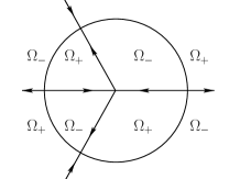
Figure 4. Contours $\Sigma_{\boldsymbol{M}}$.

$\mathbb{C}\setminus\Sigma_{\boldsymbol{M}}=\Omega_{+}\cup\Omega_{-}$, where $\Sigma_{\boldsymbol{M}}$ is positively oriented boundary of $\Omega_{+}$ and is negatively oriented boundary of $\Omega_{-}$. If $\boldsymbol{\Psi}_{\alpha,\beta}$ uniquely solves RHP-${\boldsymbol{\Psi}_{\alpha,\beta}}$, then $\boldsymbol{M}_{\alpha,\beta}$ uniquely solves the following Riemann-Hilbert problem (RHP-$\boldsymbol{M}_{\alpha,\beta}$):

• $\boldsymbol{M}_{\alpha,\beta}$ is holomorphic in $\mathbb{C}\setminus\Sigma_{\boldsymbol{M}}$ and $\boldsymbol{M}_{\alpha,\beta}(\zeta)=\boldsymbol{I}+\mathcal{O}(1/\zeta)$ as $\zeta\to\infty$;

• $\boldsymbol{M}_{\alpha,\beta}$ has continuous traces on $\Sigma_{\boldsymbol{M}}$ that satisfy $\boldsymbol{M}_{\alpha,\beta+}=\boldsymbol{M}_{\alpha,\beta-}\boldsymbol{J}$, where

  $$\boldsymbol{J}(\zeta)=\left(\boldsymbol{S}_{\alpha,\beta}(\zeta)\boldsymbol{A}_{j}e^{\theta(\zeta)\sigma_{3}}\frac{1}{\sqrt{2}}\left(\begin{matrix}1&-\mathrm{i}\\ -\mathrm{i}&1\end{matrix}\right)\zeta^{\sigma_{3}/4}\right)^{\pm 1},$$

  on $\Omega_{j}\cap\big{\{}|\zeta|=1\big{\}}$ with the exponent $1$ for $j=1,3$ and the exponent $-1$ for $j=2,4$, and on the rest of the contour $\Sigma_{\boldsymbol{M}}$ the jump is equal to

  $$\boldsymbol{J}(\zeta)=\boldsymbol{I}+e^{-2\theta(\zeta)}\left\{\begin{array}[]{rl}\boldsymbol{0},&\zeta\in\Sigma_{\boldsymbol{M}}\cap\big{\{}|\zeta|<1\big{\}}\>\text{or}\;\zeta\in(-\infty,-1),\vskip 6.0pt plus 2.0pt minus 2.0pt\\ \frac{\beta}{2}\left(\begin{matrix}-\mathrm{i}&\zeta^{-1/2}\\ \zeta^{1/2}&\mathrm{i}\end{matrix}\right),&\zeta\in(1,\infty),\vskip 6.0pt plus 2.0pt minus 2.0pt\\ \frac{e^{\pm\alpha\pi\mathrm{i}}}{2}\left(\begin{matrix}\mathrm{i}\zeta^{-1/2}&1\\ 1&-\mathrm{i}\zeta^{1/2}\end{matrix}\right),&\zeta\in I_{\pm}\cap\big{\{}|\zeta|>1\big{\}}.\end{array}\right.$$

According to [18, Appendix], see also [16, Prop. 2.4], the unique solution of RHP-$\boldsymbol{M}_{\alpha,\beta}$ is given by the formula

$$\boldsymbol{M}_{\alpha,\beta}(\zeta)=\boldsymbol{I}+\mathcal{C}\big{(}\boldsymbol{M}(\boldsymbol{W}_{+}+\boldsymbol{W}_{-})\big{)}(\zeta),\quad\zeta\in\mathbb{C}\setminus\Sigma_{\boldsymbol{M}},$$

where $\boldsymbol{J}=(\boldsymbol{I}-\boldsymbol{W}_{-})^{-1}(\boldsymbol{I}-\boldsymbol{W}_{+})$ is a factorization of the jump $\boldsymbol{J}$ for some $\boldsymbol{W}_{\pm}\in L^{2}(\Sigma_{\boldsymbol{M}})\cap L^{\infty}(\Sigma_{\boldsymbol{M}})$, $\mathcal{C}$ is a Cauchy operator

$$\mathcal{C}\boldsymbol{H}(\zeta)=\frac{1}{2\pi\mathrm{i}}\int_{\Sigma_{\boldsymbol{M}}}\frac{\boldsymbol{H}(s)}{s-\zeta}\mathrm{d}s,\quad\boldsymbol{H}\in L^{2}(\Sigma_{\boldsymbol{M}}),\quad\zeta\in\mathbb{C}\setminus\Sigma_{\boldsymbol{M}},$$

and $\boldsymbol{M}\in\boldsymbol{I}+L^{2}(\Sigma_{\boldsymbol{M}})$ is the solution of the singular integral equation

(99) $$\big{(}\mathcal{I}-\mathcal{C}_{\boldsymbol{W}}\big{)}\boldsymbol{M}=\boldsymbol{I}$$

for the singular operator $\mathcal{C}_{\boldsymbol{W}}:L^{2}(\Sigma_{\boldsymbol{M}})\to L^{2}(\Sigma_{\boldsymbol{M}})$ given by

$$\mathcal{C}_{\boldsymbol{W}}\boldsymbol{H}:=\mathcal{C}_{+}(\boldsymbol{HW}_{-})+\mathcal{C}_{-}(\boldsymbol{HW}_{+}),\quad\boldsymbol{H}\in L^{2}(\Sigma_{\boldsymbol{M}}),$$

provided this solution exists and is unique. Indeed, given such $\boldsymbol{M}$, it holds that

$$\boldsymbol{I}+\mathcal{C}_{\pm}\big{(}\boldsymbol{M}(\boldsymbol{W}_{+}+\boldsymbol{W}_{-})\big{)}=\boldsymbol{I}+\mathcal{C}_{\boldsymbol{W}}\boldsymbol{M}+\big{(}\mathcal{C}_{\pm}-\mathcal{C}_{\mp}\big{)}(\boldsymbol{MW}_{\pm})=\boldsymbol{M}\pm\boldsymbol{MW}_{\pm}$$

by (99) and Sokhotski-Pemelj formulae [13, Section 4.2]. Then

$$\left(\boldsymbol{I}+\mathcal{C}_{-}\big{(}\boldsymbol{M}(\boldsymbol{W}_{+}+\boldsymbol{W}_{-})\big{)}\right)^{-1}\left(\boldsymbol{I}+\mathcal{C}_{+}\big{(}\boldsymbol{M}(\boldsymbol{W}_{+}+\boldsymbol{W}_{-})\big{)}\right)=(\boldsymbol{I}-\boldsymbol{W}_{-})^{-1}(\boldsymbol{I}-\boldsymbol{W}_{+})=\boldsymbol{J}$$

as desired. Thus, only the unique solvability of (99) needs to be shown. The sufficient condition for the latter is bijectivity of the operator $\mathcal{I}-\mathcal{C}_{\boldsymbol{W}}$, which can be established by showing that $\mathcal{I}-\mathcal{C}_{\boldsymbol{W}}$ is Fredholm with index zero and trivial kernel.

To this end, let us specify $\boldsymbol{W}_{\pm}$. Away from the points of self-intersection of $\Sigma_{\boldsymbol{M}}$, set

$$\boldsymbol{W}_{+}:=\boldsymbol{J}-\boldsymbol{I}\quad\text{and}\quad\boldsymbol{W}_{-}=\boldsymbol{0}.$$

Around the points of self-intersection, we chose $\boldsymbol{W}_{+}$ to be continuous along the boundary of $\Omega_{+}$ and $\boldsymbol{W}_{-}$ to be continuous along the boundary of $\Omega_{-}$. The latter is possible because around each point of self-intersection of $\Sigma_{\boldsymbol{M}}$, the jumps satisfy the cyclic relation

$$\boldsymbol{J}_{1}\boldsymbol{J}_{2}^{-1}\boldsymbol{J}_{3}\boldsymbol{J}_{4}^{-1}=\boldsymbol{I},$$

where we label the four arcs meeting at the point of self-intersection counter-clockwise starting with an arc oriented away from the point and denote by $\boldsymbol{J}_{i}$ the jump across the $i$-th arc. Clearly, $\boldsymbol{W}_{\pm}\in L^{2}(\Sigma_{\boldsymbol{M}})\cap L^{\infty}(\Sigma_{\boldsymbol{M}})$. To show that $\mathcal{I}-\mathcal{C}_{\boldsymbol{W}}$ is Fredholm, one needs to construct its pseudoinverse. The latter is given by $\mathcal{I}-\mathcal{C}_{\widetilde{\boldsymbol{W}}}$, where

$$\widetilde{\boldsymbol{W}}_{+}:=\big{(}\boldsymbol{I}+\boldsymbol{W}_{+}\big{)}^{-1}-\boldsymbol{I}\quad\text{and}\quad\widetilde{\boldsymbol{W}}_{-}:=\boldsymbol{I}-\big{(}\boldsymbol{I}-\boldsymbol{W}_{-}\big{)}^{-1},$$

as explained in [16, Eq. (2.39)–(2.42)]. The index of $\mathcal{I}-\mathcal{C}_{\boldsymbol{W}}$ is equal to the winding number of $\mathsf{det}(\boldsymbol{J})$, which is zero since $\mathsf{det}(\boldsymbol{J})\equiv 1$. Finally, the kernel of $\mathcal{I}-\mathcal{C}_{\boldsymbol{W}}$ is trivial if and only if the homogeneous Riemann-Hilbert problem corresponding to RHP-$\boldsymbol{M}_{\alpha,\beta}$ has only trivial solutions. Correspondence between RHP-${\boldsymbol{\Psi}_{\alpha,\beta}}$ and RHP-$\boldsymbol{M}_{\alpha,\beta}$ implies that the kernel is trivial if and only if the solution of RHP-${\boldsymbol{\Psi}_{\alpha,\beta}}$ with RHP-${\boldsymbol{\Psi}_{\alpha,\beta}}$(d) replaced by (97) has only trivial solutions. This is precisely the content of the preceding subsection. This finishes the proof of the first claim of Theorem 7.

10.5   Asymptotics of RHP-${\boldsymbol{\Psi}_{\alpha,\beta}}$ for $s>0$

It is known that $\mathcal{O}\left(\eta^{-1}\right)$ is uniform for $s$ on compact subsets of the real line [16]. Thus, we only need to prove (33) for $s$ large.

10.5.1   Renormalized RHP-${\boldsymbol{\Psi}_{\alpha,\beta}}$

Set $\widehat{I}_{\pm}:=\{\eta:\mathsf{arg}(\eta+1)=\pm 2\pi/3\}$ and let $\widehat{\Omega}_{j}$, $j\in\{1,2,3,4\}$, be the domains comprising $\mathbb{C}\setminus\big{(}(-\infty,\infty)\cup\widehat{I}_{+}\cup\widehat{I}_{-}\big{)}$, numbered counter-clockwise and so that $\widehat{\Omega}_{1}$ contains the first quadrant. Define

$$g(\eta)=\frac{2}{3}(\eta+1)^{3/2},\quad\eta\in\mathbb{C}\setminus(-\infty,-1],$$

to be the principal branch and set for convenience $\tau:=s^{3/2}$. Let

(100) $$\widehat{\boldsymbol{\Psi}}_{\alpha,\beta}(\eta;\tau)=s^{\sigma_{3}/4}\boldsymbol{\Psi}_{\alpha,\beta}(s\eta;s)\left\{\begin{array}[]{lll}\boldsymbol{I}&\text{in}&\Omega_{1}\cup\Omega_{4}\cup\widehat{\Omega}_{2}\cup\widehat{\Omega}_{3},\vskip 6.0pt plus 2.0pt minus 2.0pt\\ \left(\begin{matrix}1&0\\ \pm e^{\pm\alpha\pi\mathrm{i}}&1\end{matrix}\right)&\text{in}&\Omega_{2}\setminus\widehat{\Omega}_{2},\;\Omega_{3}\setminus\widehat{\Omega}_{3},\end{array}\right.$$

where the sign $+$ is used in $\Omega_{2}\setminus\widehat{\Omega}_{2}$ and the sign $-$ in $\Omega_{3}\setminus\widehat{\Omega}_{3}$. Then $\widehat{\boldsymbol{\Psi}}_{\alpha,\beta}$ solves the following Riemann-Hilbert problem (RHP-${\widehat{\boldsymbol{\Psi}}_{\alpha,\beta}}$):

• $\widehat{\boldsymbol{\Psi}}_{\alpha,\beta}$ is holomorphic in $\mathbb{C}\setminus\big{(}\widehat{I}_{+}\cup\widehat{I}_{-}\cup(-\infty,\infty)\big{)}$;

• $\widehat{\boldsymbol{\Psi}}_{\alpha,\beta}$ has continuous traces on $\widehat{I}_{+}\cup\widehat{I}_{-}\cup(-\infty,-1)\cup(-1,0)\cup(0,\infty)$ that satisfy

  $$\widehat{\boldsymbol{\Psi}}_{\alpha,\beta+}=\widehat{\boldsymbol{\Psi}}_{\alpha,\beta-}\left\{\begin{array}[]{rll}\left(\begin{matrix}0&1\\ -1&0\end{matrix}\right)&\text{on}&(-\infty,-1),\vskip 6.0pt plus 2.0pt minus 2.0pt\\ \left(\begin{matrix}e^{\alpha\pi\mathrm{i}}&1\\ 0&e^{-\alpha\pi\mathrm{i}}\end{matrix}\right)&\text{on}&(-1,0),\vskip 6.0pt plus 2.0pt minus 2.0pt\\ \left(\begin{matrix}1&\beta\\ 0&1\end{matrix}\right)&\text{on}&(0,\infty),\vskip 6.0pt plus 2.0pt minus 2.0pt\\ \left(\begin{matrix}1&0\\ e^{\pm\alpha\pi\mathrm{i}}&1\end{matrix}\right)&\text{on}&\widehat{I}_{\pm};\end{array}\right.$$

• as $\eta\to 0$ it holds that

  $$\widehat{\boldsymbol{\Psi}}_{\alpha,\beta}(\eta;\tau)=\widehat{\boldsymbol{E}}(\eta)\boldsymbol{S}_{\alpha,\beta}(\eta)\boldsymbol{A}_{j},\quad\eta\in\widehat{\Omega}_{j},\quad j\in\{1,4\},$$

  where $\widehat{\boldsymbol{E}}$ is holomorphic, and $\boldsymbol{S}_{\alpha,\beta}$, $\boldsymbol{A}_{1}$ and $\boldsymbol{A}_{4}$ are the same as in RHP-${\boldsymbol{\Psi}_{\alpha,\beta}}$(c);

• $\widehat{\boldsymbol{\Psi}}_{\alpha,\beta}$ has the following behavior near $\infty$:

  $$\widehat{\boldsymbol{\Psi}}_{\alpha,\beta}(\eta;\tau)=\left(\boldsymbol{I}+\mathcal{O}\left(\eta^{-1}\right)\right)\frac{\eta^{-\sigma_{3}/4}}{\sqrt{2}}\left(\begin{matrix}1&\mathrm{i}\\ \mathrm{i}&1\end{matrix}\right)e^{-\tau g(\eta)\sigma_{3}}$$

  uniformly in $\mathbb{C}\setminus\big{(}\widehat{I}_{+}\cup\widehat{I}_{-}\cup(-\infty,\infty)\big{)}$.

10.5.2   Global Parametrix

Let

$$\widehat{\boldsymbol{\Psi}}^{(\infty)}(\eta;\tau) := \left(\begin{matrix}1&0\\ \alpha\mathrm{i}&1\end{matrix}\right)\frac{(\eta+1)^{-\sigma_{3}/4}}{\sqrt{2}}\left(\begin{matrix}1&\mathrm{i}\\ \mathrm{i}&1\end{matrix}\right)\left(\frac{(\eta+1)^{1/2}+1}{(\eta+1)^{1/2}-1}\right)^{-\alpha\sigma_{3}/2}e^{-\tau g(\eta)\sigma_{3}}$$

$$=: \boldsymbol{F}^{(\infty)}(\tau)e^{-\tau g(\eta)\sigma_{3}}.$$

Then, as is explained in [17, Section 2.4.1], this matrix-valued function solves the following Riemann-Hilbert problem:

• $\widehat{\boldsymbol{\Psi}}^{(\infty)}$ is holomorphic in $\mathbb{C}\setminus(-\infty,0]$;

• $\widehat{\boldsymbol{\Psi}}^{(\infty)}$ has continuous traces on $(-\infty,-1)\cup(-1,0)$ that satisfy

  $$\widehat{\boldsymbol{\Psi}}_{+}^{(\infty)}=\widehat{\boldsymbol{\Psi}}_{-}^{(\infty)}\left\{\begin{array}[]{rll}\left(\begin{matrix}0&1\\ -1&0\end{matrix}\right)&\text{on}&(-\infty,-1),\vskip 6.0pt plus 2.0pt minus 2.0pt\\ e^{\alpha\pi\mathrm{i}\sigma_{3}}&\text{on}&(-1,0),\end{array}\right.$$

• as $\eta\to 0$ it holds that $\widehat{\boldsymbol{\Psi}}^{(\infty)}(\eta;\tau)=\widehat{\boldsymbol{E}}^{(\infty)}(\eta)\eta^{\alpha\sigma_{3}/2}$, where $\widehat{\boldsymbol{E}}^{(\infty)}$ is holomorphic and non-vanishing around zero;

• $\widehat{\boldsymbol{\Psi}}^{(\infty)}$ satisfies RHP-${\widehat{\boldsymbol{\Psi}}_{\alpha,\beta}}$(d) uniformly in $\mathbb{C}\setminus(-\infty;0]$ and the term $\mathcal{O}\big{(}\eta^{-1}\big{)}$ does not depend on $\tau$.

Notice that $\boldsymbol{F}^{(\infty)}$ has the same jumps as $\widehat{\boldsymbol{\Psi}}^{(\infty)}$.

10.5.3   Local Parametrix Around $-1$

The solution $\boldsymbol{\Psi}_{\mathsf{Ai}}:=\boldsymbol{\Psi}_{0,1}(\cdot;0)$ is known explicitly and is constructed with the help of the Airy function and its derivative [9]. Set

$$\widehat{\boldsymbol{\Psi}}^{(-1)}(\eta;\tau):=\widehat{\boldsymbol{E}}^{(-1)}(\eta)\boldsymbol{\Psi}_{\mathsf{Ai}}\big{(}s(\eta+1)\big{)}e^{\pm\alpha\pi\mathrm{i}\sigma_{3}/2},\quad\pm\mathsf{Im}(\eta)>0,$$

where $\widehat{\boldsymbol{E}}^{(-1)}$ is holomorphic around $-1$ and is given by

$$\widehat{\boldsymbol{E}}^{(-1)}(\eta):=\boldsymbol{F}^{(\infty)}(\eta)\left(\frac{\big{(}s(\eta+1)\big{)}^{-\sigma_{3}/4}}{\sqrt{2}}\left(\begin{matrix}1&\mathrm{i}\\ \mathrm{i}&1\end{matrix}\right)e^{\pm\alpha\pi\mathrm{i}\sigma_{3}/2}\right)^{-1},\quad\pm\mathsf{Im}(\eta)>0.$$

Let $U_{-1}$ be the disk of radius $1/4$ centered at $-1$ with boundary oriented counter-clockwise. Then it is shown in [17, Section 2.4.2] that $\widehat{\boldsymbol{\Psi}}^{(-1)}$ satisfies

• $\widehat{\boldsymbol{\Psi}}^{(-1)}$ is holomorphic in $U_{-1}\setminus\big{(}\widehat{I}_{+}\cup\widehat{I}_{-}\cup(-\infty,\infty)\big{)}$;

• $\widehat{\boldsymbol{\Psi}}^{(-1)}$ has continuous traces on $U_{-1}\cap\big{(}\widehat{I}_{+}\cup\widehat{I}_{-}\cup(-\infty,\infty)\big{)}$ that satisfy RHP-${\widehat{\boldsymbol{\Psi}}_{\alpha,\beta}}$(b);

• it holds that

  $$\widehat{\boldsymbol{\Psi}}^{(-1)}(\eta;\tau)=\boldsymbol{F}^{(\infty)}(\eta)\left(\boldsymbol{I}+\mathcal{O}\left(\tau^{-1}\right)\right)e^{-\tau g(\eta)\sigma_{3}}$$

  as $\tau\to\infty$, uniformly for $\eta\in\partial U_{-1}\setminus\big{(}\widehat{I}_{+}\cup\widehat{I}_{-}\cup(-\infty,\infty)\big{)}$.

10.5.4   Local Parametrix Around $0$

Define

$$\widehat{\boldsymbol{\Psi}}^{(0)}(\eta;\tau):=\widehat{\boldsymbol{E}}^{(0)}(\eta)\boldsymbol{S}_{\alpha,\beta}(\tau)\left\{\begin{array}[]{ll}\boldsymbol{A}_{1},&\mathsf{Im}(\eta)>0,\vskip 6.0pt plus 2.0pt minus 2.0pt\\ \boldsymbol{A}_{4},&\mathsf{Im}(\eta)<0,\end{array}\right.$$

where $\boldsymbol{S}_{\alpha,\beta}$ and $\boldsymbol{A}_{j}$ are the same as in RHP-${\boldsymbol{\Psi}_{\alpha,\beta}}$(c) and

$$\widehat{\boldsymbol{E}}^{(0)}(\eta):=\widehat{\boldsymbol{\Psi}}^{(\infty)}(\eta;\tau)\eta^{-\alpha\sigma_{3}/2}\left(\begin{matrix}[\boldsymbol{A}_{1}]_{11}^{-1}&0\vskip 6.0pt plus 2.0pt minus 2.0pt\\ 0&[\boldsymbol{A}_{1}]_{22}^{-1}\end{matrix}\right),$$

which is a holomorphic function around the origin by the properties of $\widehat{\boldsymbol{\Psi}}^{(\infty)}$. Let $U_{0}$ be the disk of radius $1/4$ centered at $0$ with boundary oriented counter-clockwise. Then $\widehat{\boldsymbol{\Psi}}^{(0)}$ possesses the following properties:

• $\widehat{\boldsymbol{\Psi}}^{(0)}$ is holomorphic in $U_{0}\setminus(-1/4,1/4)$;

• $\widehat{\boldsymbol{\Psi}}^{(0)}$ has continuous traces on $(-1/4,0)\cup(0,1/4)$ that satisfy RHP-${\widehat{\boldsymbol{\Psi}}_{\alpha,\beta}}$(b);

• $\widehat{\boldsymbol{\Psi}}^{(0)}$ satisfies RHP-${\widehat{\boldsymbol{\Psi}}_{\alpha,\beta}}$(c) with $\widehat{\boldsymbol{E}}$ replaced by $\widehat{\boldsymbol{E}}^{(0)}$;

• it holds that

  $$\widehat{\boldsymbol{\Psi}}^{(0)}(\eta;\tau)=\boldsymbol{F}^{(\infty)}(\eta)\left(\boldsymbol{I}+\mathcal{O}\left(e^{-c\tau}\right)\right)e^{-\tau g(\eta)\sigma_{3}}$$

  as $\tau\to\infty$ for some $c>0$, uniformly for $\eta\in\partial U_{0}\setminus\{-1/4,1/4\}$.

Indeed, properties (a,b,c) easily follow from RHP-${\widehat{\boldsymbol{\Psi}}_{\alpha,\beta}}$(b,c) and the holomorphy of $\widehat{\boldsymbol{E}}^{(0)}$. To get (d), write $[\boldsymbol{S}_{\alpha,\beta}]_{12}(\eta)=\eta^{\alpha/2}\kappa(\eta)$, where

$$\kappa(\eta)=0,\quad\kappa(\eta)=\frac{1-\beta}{2\pi\mathrm{i}}\log\eta,\quad\text{or}\quad\kappa(\eta)=\frac{1+\beta}{2\pi\mathrm{i}}\log\eta$$

depending on whether $\alpha$ is not an integer, an even integer, or an odd integer. Recall also that $\boldsymbol{A}_{1}$ and $\boldsymbol{A}_{4}$ are upper triangular matrices and $[\boldsymbol{A}_{1}]_{ii}=[\boldsymbol{A}_{4}]_{ii}$ for $i\in\{1,2\}$. Then

$$\widehat{\boldsymbol{\Psi}}^{(0)}(\eta;\tau) = \boldsymbol{F}^{(\infty)}(\eta)e^{-\tau g(\eta)\sigma_{3}}\left(\begin{matrix}[\boldsymbol{A}_{j}]_{11}^{-1}&0\vskip 6.0pt plus 2.0pt minus 2.0pt\\ 0&[\boldsymbol{A}_{j}]_{22}^{-1}\end{matrix}\right)\left(\begin{matrix}1&\kappa(\eta)\vskip 6.0pt plus 2.0pt minus 2.0pt\\ 0&1\end{matrix}\right)\boldsymbol{A}_{j}$$

$$= \boldsymbol{F}^{(\infty)}(\eta)\left(\begin{matrix}1&e^{-2\tau g(\eta)}\big{(}[\boldsymbol{A}_{j}]_{22}\kappa(\eta)+[\boldsymbol{A}_{j}]_{12}\big{)}/[\boldsymbol{A}_{j}]_{11}\vskip 6.0pt plus 2.0pt minus 2.0pt\\ 0&1\end{matrix}\right)e^{-\tau g(\eta)\sigma_{3}},$$

from which property (d) can be easily deduced as $\tau>0$ and $\mathsf{Re}(g(\eta))>0$ for $\eta\in\partial U_{0}$.

10.5.5   Asymptotics of RHP-${\boldsymbol{\Psi}_{\alpha,\beta}}$

Denote by

$$\Sigma(\boldsymbol{R}_{\alpha,\beta}):=\partial U_{-1}\cup\partial U_{0}\cup\left(\big{(}\widehat{I}_{-}\cup\widehat{I}_{+}\cup(-1,\infty)\big{)}\cap\left(\mathbb{C}\setminus\big{(}\overline{U}_{-1}\cup\overline{U}_{0}\big{)}\right)\right),$$

and let $\Sigma^{\circ}(\boldsymbol{R}_{\alpha,\beta})$ be $\Sigma(\boldsymbol{R}_{\alpha,\beta})$ with the points of self-intersection removed. Put

$$\boldsymbol{R}_{\alpha,\beta}(\eta;\tau):=\widehat{\boldsymbol{\Psi}}_{\alpha,\beta}(\eta;\tau)\left\{\begin{array}[]{ll}\widehat{\boldsymbol{\Psi}}^{(-1)}(\eta;\tau)^{-1},&\eta\in U_{-1},\vskip 6.0pt plus 2.0pt minus 2.0pt\\ \widehat{\boldsymbol{\Psi}}^{(0)}(\eta;\tau)^{-1},&\eta\in U_{0},\vskip 6.0pt plus 2.0pt minus 2.0pt\\ \widehat{\boldsymbol{\Psi}}^{(\infty)}(\eta;\tau)^{-1},&\eta\in\mathbb{C}\setminus\big{(}\overline{U}_{0}\cup\overline{U}_{-1}\big{)}.\end{array}\right.$$

Then $\boldsymbol{R}_{\alpha,\beta}$ has the following properties:

• $\boldsymbol{R}_{\alpha,\beta}$ is holomorphic in $\mathbb{C}\setminus\Sigma(\boldsymbol{R}_{\alpha,\beta})$;

• $\boldsymbol{R}_{\alpha,\beta}$ has continuous traces on $\Sigma^{\circ}(\boldsymbol{R}_{\alpha,\beta})$ that satisfy $\boldsymbol{R}_{\alpha,\beta+}^{(0)}:=\boldsymbol{R}_{\alpha,\beta-}^{(0)}\left(\boldsymbol{I}+\mathcal{O}\left(\tau^{-1}\right)\right)$ as $\tau\to\infty$;

• it holds that $\boldsymbol{R}_{\alpha,\beta}(\eta;\tau)=\boldsymbol{I}+\mathcal{O}\left(\eta^{-1}\right)$ as $\eta\to\infty$ uniformly in $\mathbb{C}\setminus\Sigma(\boldsymbol{R}_{\alpha,\beta})$.

Property (a) follows from the facts that $\widehat{\boldsymbol{\Psi}}^{(e)}$ has the same jumps as $\widehat{\boldsymbol{\Psi}}_{\alpha,\beta}$ in $U_{e}$, $e\in\{-1,0\}$, $\widehat{\boldsymbol{\Psi}}^{(\infty)}$ has the same jump across $(-\infty,-1)$ as $\widehat{\boldsymbol{\Psi}}_{\alpha,\beta}$, and $\widehat{\boldsymbol{\Psi}}^{(0)}$ has the same local behavior around $0$ as $\widehat{\boldsymbol{\Psi}}_{\alpha,\beta}$. Property (c) follows easily from the fact that both $\widehat{\boldsymbol{\Psi}}^{(\infty)}$ and $\widehat{\boldsymbol{\Psi}}_{\alpha,\beta}$ satisfy RHP-${\widehat{\boldsymbol{\Psi}}_{\alpha,\beta}}$(d). Property (b) on $\partial U_{e}$, $e\in\{-1,0\}$, is the consequence of the fact

$$\boldsymbol{R}_{\alpha,\beta-}^{-1}\boldsymbol{R}_{\alpha,\beta+}=\widehat{\boldsymbol{\Psi}}^{(\infty)}\widehat{\boldsymbol{\Psi}}^{(e)-1}=\boldsymbol{I}+\boldsymbol{F}^{(\infty)}\mathcal{O}\left(\tau^{-1}\right)\boldsymbol{F}^{(\infty)-1}.$$

Finally, on the rest of $\Sigma(\boldsymbol{R}_{\alpha,\beta})$ it holds that

$$\boldsymbol{R}_{\alpha,\beta+}=\boldsymbol{R}_{\alpha,\beta-}\left\{\begin{array}[]{lll}\boldsymbol{I}+\boldsymbol{F}_{-}^{(\infty)}\left(\begin{matrix}0&e^{-2\tau g}\\ 0&0\end{matrix}\right)\boldsymbol{F}_{+}^{(\infty)-1}&\text{on}&(-3/4,-1/4),\vskip 6.0pt plus 2.0pt minus 2.0pt\\ \boldsymbol{I}+\boldsymbol{F}^{(\infty)}\left(\begin{matrix}0&\beta e^{-2\tau g}\\ 0&0\end{matrix}\right)\boldsymbol{F}^{(\infty)-1}&\text{on}&(1/4,\infty),\vskip 6.0pt plus 2.0pt minus 2.0pt\\ \boldsymbol{I}+\boldsymbol{F}^{(\infty)}\left(\begin{matrix}0&0\\ e^{\pm\alpha\pi\mathrm{i}}e^{2\tau g}&0\end{matrix}\right)\boldsymbol{F}^{(\infty)-1}&\text{on}&\widehat{I}_{\pm}\setminus\overline{U}_{-1}.\end{array}\right.$$

As $g(\eta)>0$ for $\eta\in(-1,\infty)$ and $g(\eta)<0$ for $\eta\in\widehat{I}_{\pm}$, the last part of the property (b) follows. Given (a,b,c) it is by now standard to conclude that

$$\boldsymbol{R}_{\alpha,\beta}(\eta;\tau)=\boldsymbol{I}+\mathcal{O}\left(\frac{1}{\tau(1+|\eta|)}\right)$$

as $\tau\to\infty$ uniformly for $\eta\in\mathbb{C}\setminus\Sigma(\boldsymbol{R}_{\alpha,\beta})$. Thus,

(101) $$\widehat{\boldsymbol{\Psi}}_{\alpha,\beta}(\eta;\tau) = \frac{\eta^{-\sigma_{3}/4}}{\sqrt{2}}\left(\boldsymbol{I}+\mathcal{O}\left(\frac{1}{\tau\sqrt{1+|\eta|}}\right)\right)\left(\boldsymbol{I}+\mathcal{O}\left(\eta^{-1/2}\right)\right)\left(\begin{matrix}1&\mathrm{i}\\ \mathrm{i}&1\end{matrix}\right)e^{-\tau g(\eta)\sigma_{3}}$$

$$= \frac{\eta^{-\sigma_{3}/4}}{\sqrt{2}}\left(\boldsymbol{I}+\mathcal{O}\left(\eta^{-1/2}\right)\right)\left(\begin{matrix}1&\mathrm{i}\\ \mathrm{i}&1\end{matrix}\right)e^{-\tau g(\eta)\sigma_{3}}$$

as $\eta\to\infty$ uniformly for $\eta\in\mathbb{C}\setminus\Sigma(\boldsymbol{R}_{\alpha,\beta})$ and $\tau$ large. Estimate (33) now follows from (100).

10.6   Asymptotics of RHP-${\boldsymbol{\Psi}_{\alpha,\beta}}$ for $s<0$

In this section we assume that $\beta\neq 0$ and define

$$\log\beta=\log|\beta|+\mathrm{i}\mathsf{arg}(\beta),\quad\mathsf{arg}(\beta)\in(-\pi,\pi).$$

Again, we only need to prove (33) when $s\to-\infty$.

10.6.1   Renormalized RHP-${\boldsymbol{\Psi}_{\alpha,\beta}}$

Set $\widehat{J}_{\pm}$ to be two Jordan arcs connecting $0$ and $1$, oriented from $0$ to $1$, and lying in the first $(+)$ and the fourth ($-$) quadrants. Denote further by $\Omega_{\pm}$ the domains delimited by $\widehat{J}_{\pm}$ and $[0,1]$. Define

$$g(\eta)=\frac{2}{3}(\eta-1)^{3/2},\quad\eta\in\mathbb{C}\setminus(-\infty,1],$$

to be the principal branch and set for convenience $\tau:=(-s)^{3/2}$. Let

(102) $$\widehat{\boldsymbol{\Psi}}_{\alpha,\beta}(\eta;\tau)=(-s)^{\sigma_{3}/4}\boldsymbol{\Psi}_{\alpha,\beta}(-s\eta;s)\left\{\begin{array}[]{lr}\left(\begin{matrix}1&0\\ \mp 1/\beta&1\end{matrix}\right)&\text{in}\quad\Omega_{\pm},\vskip 6.0pt plus 2.0pt minus 2.0pt\\ \boldsymbol{I}&\text{otherwise}.\end{array}\right.$$

Put for brevity $\Sigma(\widehat{\boldsymbol{\Psi}}_{\alpha,\beta}):=I_{+}\cup I_{-}\cup(-\infty,\infty)\cup\widehat{J}_{+}\cup\widehat{J}_{-}$. Then $\widehat{\boldsymbol{\Psi}}_{\alpha,\beta}$ solves the following Riemann-Hilbert problem (RHP-${\widehat{\boldsymbol{\Psi}}_{\alpha,\beta}}$):

• $\widehat{\boldsymbol{\Psi}}_{\alpha,\beta}$ is holomorphic in $\mathbb{C}\setminus\Sigma(\widehat{\boldsymbol{\Psi}}_{\alpha,\beta})$;

• $\widehat{\boldsymbol{\Psi}}_{\alpha,\beta}$ has continuous traces on $\Sigma(\widehat{\boldsymbol{\Psi}}_{\alpha,\beta})\setminus\{0,1\}$ that satisfy

  $$\widehat{\boldsymbol{\Psi}}_{\alpha,\beta+}=\widehat{\boldsymbol{\Psi}}_{\alpha,\beta-}\left\{\begin{array}[]{rll}\left(\begin{matrix}0&1\\ -1&0\end{matrix}\right)&\text{on}&(-\infty,0),\vskip 6.0pt plus 2.0pt minus 2.0pt\\ \left(\begin{matrix}0&\beta\\ -1/\beta&0\end{matrix}\right)&\text{on}&(0,1),\vskip 6.0pt plus 2.0pt minus 2.0pt\\ \left(\begin{matrix}1&\beta\\ 0&1\end{matrix}\right)&\text{on}&(1,\infty),\vskip 6.0pt plus 2.0pt minus 2.0pt\\ \end{array}\right.$$

  and

  $$\widehat{\boldsymbol{\Psi}}_{\alpha,\beta+}=\widehat{\boldsymbol{\Psi}}_{\alpha,\beta-}\left\{\begin{array}[]{rll}\left(\begin{matrix}1&0\\ 1/\beta&1\end{matrix}\right)&\text{on}&\widehat{J}_{\pm},\vskip 6.0pt plus 2.0pt minus 2.0pt\\ \left(\begin{matrix}1&0\\ e^{\pm\alpha\pi\mathrm{i}}&1\end{matrix}\right)&\text{on}&I_{\pm};\end{array}\right.$$

• as $\eta\to 0$ it holds that

  $$\widehat{\boldsymbol{\Psi}}_{\alpha,\beta}(\eta;\tau)=\mathcal{O}\left(\begin{matrix}|\zeta|^{\alpha/2}&|\zeta|^{\alpha/2}+|\zeta|^{-\alpha/2}\\ |\zeta|^{\alpha/2}&|\zeta|^{\alpha/2}+|\zeta|^{-\alpha/2}\end{matrix}\right)\quad\text{and}\quad\widehat{\boldsymbol{\Psi}}_{\alpha,\beta}(\eta;\tau)=\mathcal{O}\left(\begin{matrix}1&\log|\zeta|\\ 1&\log|\zeta|\end{matrix}\right)$$

  when $\alpha\neq 0$ and $\alpha=0$, respectively;

• $\widehat{\boldsymbol{\Psi}}_{\alpha,\beta}$ has the following behavior near $\infty$:

  $$\widehat{\boldsymbol{\Psi}}_{\alpha,\beta}(\eta;\tau)=\left(\boldsymbol{I}+\mathcal{O}\left(\eta^{-1}\right)\right)\frac{\eta^{-\sigma_{3}/4}}{\sqrt{2}}\left(\begin{matrix}1&\mathrm{i}\\ \mathrm{i}&1\end{matrix}\right)e^{-\tau g(\eta)\sigma_{3}}$$

  uniformly in $\mathbb{C}\setminus\big{(}I_{+}\cup I_{-}\cup(-\infty,\infty)\big{)}$.

10.6.2   Global Parametrix

Set

$$\widehat{\boldsymbol{\Psi}}^{(\infty)}(\eta;\tau):=\boldsymbol{F}^{(\infty)}(\eta)e^{-\tau g(\eta)\sigma_{3}},$$

where

$$\boldsymbol{F}^{(\infty)}(\eta):=\left(\begin{matrix}1&0\\ -\frac{1}{\pi\mathrm{i}}\log\beta&1\end{matrix}\right)\frac{(\eta-1)^{-\sigma_{3}/4}}{\sqrt{2}}\left(\begin{matrix}1&\mathrm{i}\\ \mathrm{i}&1\end{matrix}\right)F_{\beta}^{-\sigma_{3}}(\eta)$$

and the function $F_{\beta}$ is give by (83). Now, it is a straightforward verification to see that

• $\widehat{\boldsymbol{\Psi}}^{(\infty)}$ is holomorphic in $\mathbb{C}\setminus(-\infty,1]$;

• $\widehat{\boldsymbol{\Psi}}^{(\infty)}$ has continuous traces on $(-\infty,1)$ that satisfy

  $$\widehat{\boldsymbol{\Psi}}_{+}^{(\infty)}=\widehat{\boldsymbol{\Psi}}_{-}^{(\infty)}\left\{\begin{array}[]{rll}\left(\begin{matrix}0&1\\ -1&0\end{matrix}\right)&\text{on}&(-\infty,0),\vskip 6.0pt plus 2.0pt minus 2.0pt\\ \left(\begin{matrix}0&\beta\\ -1/\beta&0\end{matrix}\right)&\text{on}&(0,1);\end{array}\right.$$

• $\widehat{\boldsymbol{\Psi}}^{(\infty)}$ satisfies RHP-${\widehat{\boldsymbol{\Psi}}_{\alpha,\beta}}$(d) uniformly in $\mathbb{C}\setminus(-\infty;1]$ and the term $\mathcal{O}\big{(}\eta^{-1}\big{)}$ does not depend on $\tau$.

Again, notice that $\widehat{\boldsymbol{\Psi}}^{(\infty)}$ and $\boldsymbol{F}^{(\infty)}$ satisfy the same jump relations.

10.6.3   Local Parametrix Around $1$

Denote by $U_{1}$ the disk centered at $1$ of radius $1/4$ with boundary oriented counter-clockwise. Choose arcs $\widehat{J}_{\pm}$ so that

$$\big{\{}\eta-1:~{}\eta\in\widehat{J}_{\pm}\cap U_{1}\big{\}}\subset I_{\pm}.$$

Let, as before, $\boldsymbol{\Psi}_{\mathsf{Ai}}=\boldsymbol{\Psi}_{0,1}(\cdot;0)$. Set

$$\widehat{\boldsymbol{\Psi}}^{(1)}(\eta;\tau):=\widehat{\boldsymbol{E}}^{(1)}(\eta)\boldsymbol{\Psi}_{\mathsf{Ai}}\big{(}-s(\eta-1)\big{)}\beta^{-\sigma_{3}/2},$$

where $\widehat{\boldsymbol{E}}^{(1)}$ is holomorphic around $1$ and is given by

$$\widehat{\boldsymbol{E}}^{(1)}(\eta):=\boldsymbol{F}^{(\infty)}(\eta)\left(\frac{\big{(}-s(\eta-1)\big{)}^{-\sigma_{3}/4}}{\sqrt{2}}\left(\begin{matrix}1&\mathrm{i}\\ \mathrm{i}&1\end{matrix}\right)\beta^{-\sigma_{3}/2}\right)^{-1}.$$

Then it can be checked that $\widehat{\boldsymbol{\Psi}}^{(1)}$ satisfies

• $\widehat{\boldsymbol{\Psi}}^{(1)}$ is holomorphic in $U_{1}\setminus\Sigma(\widehat{\boldsymbol{\Psi}}_{\alpha,\beta})$;

• $\widehat{\boldsymbol{\Psi}}^{(1)}$ has continuous traces on $U_{1}\cap\Sigma(\widehat{\boldsymbol{\Psi}}_{\alpha,\beta})$ that satisfy RHP-${\widehat{\boldsymbol{\Psi}}_{\alpha,\beta}}$(b);

• it holds that

  $$\widehat{\boldsymbol{\Psi}}^{(1)}(\eta;\tau)=\boldsymbol{F}^{(\infty)}(\eta)\left(\boldsymbol{I}+\mathcal{O}\left(\tau^{-1}\right)\right)e^{-\tau g(\eta)\sigma_{3}}$$

  as $\tau\to\infty$, uniformly for $\eta\in\partial U_{1}\setminus\Sigma(\widehat{\boldsymbol{\Psi}}_{\alpha,\beta})$.

10.6.4   Local Parametrix Around $0$

Denote by $U_{0}$ the disk centered at $0$ of radius $1/4$ whose boundary oriented counter-clockwise. Let

$$m(\eta):=3\mp 2\mathrm{i}g(\eta),\quad\pm\mathsf{Im}(\eta)>0.$$

Then $m$ is conformal in $U_{0}$, $m(0)=0$, and $m(x)>0$ for $x\in(0,1/4)$. Choose the arcs $\widehat{J}_{\pm}$ so that $m\big{(}\widehat{J}_{\pm}\big{)}\subset J_{\pm}$. Define

$$\widehat{\boldsymbol{\Psi}}^{(0)}(\eta;\tau):=\widehat{\boldsymbol{E}}^{(0)}(\eta)\mathcal{D}\left(\boldsymbol{\Phi}_{\alpha,\beta}\big{(}\tau m(\eta)\big{)}\right),$$

where $\boldsymbol{\Phi}_{\alpha,\beta}$ is the solution of RHP-${\boldsymbol{\Phi}_{\alpha,\beta}}$, $\mathcal{D}\left(\boldsymbol{\Phi}_{\alpha,\beta}\big{(}\tau m\big{)}\right)$ is a holomorphic deformation of $\boldsymbol{\Phi}_{\alpha,\beta}\big{(}\tau m\big{)}$ that moves the jumps from $(\tau m)^{-1}\big{(}I_{\pm}\big{)}$ to $I_{\pm}$, and $\widehat{\boldsymbol{E}}^{(0)}$ is holomorphic around $0$ and is given by

(103) $$\widehat{\boldsymbol{E}}^{(0)}(\eta):=\boldsymbol{F}^{(\infty)}(\eta)\left(e^{-3\tau\mathrm{i}\sigma_{3}/2}\big{(}\mathrm{i}\tau m(\eta)\big{)}^{\log\beta\sigma_{3}/2\pi\mathrm{i}}\boldsymbol{B}_{\pm}\right)^{-1}$$

(the constant matrices $\boldsymbol{B}_{\pm}$ were also defined in RHP-${\boldsymbol{\Phi}_{\alpha,\beta}}$). To see that $E^{(0)}$ is indeed holomorphic recall that

$$\boldsymbol{B}_{+}=\boldsymbol{B}_{-}\left(\begin{matrix}0&1\\ -1&0\end{matrix}\right)\quad\text{and}\quad\big{(}\mathrm{i}x\big{)}_{-}^{\log\beta/2\pi\mathrm{i}}=\beta\big{(}\mathrm{i}x\big{)}_{+}^{\log\beta/2\pi\mathrm{i}}$$

for $x>0$, which implies that the function in parenthesis in (103) has the same jump as $\boldsymbol{F}^{(\infty)}$ on $(-1/4,1/4)$. Observe further that

$$\boldsymbol{B}_{\pm}e^{\mp\mathrm{i}\tau m(\eta)\sigma_{3}/2}=e^{3\tau\mathrm{i}\sigma_{3}/2}\boldsymbol{B}_{\pm}e^{-\tau g(\eta)\sigma_{3}},\quad\pm\mathsf{Im}(\eta)>0.$$

Therefore, it follows from RHP-${\boldsymbol{\Phi}_{\alpha,\beta}}$(d) that

$$\widehat{\boldsymbol{\Psi}}^{(0)}(\eta;\tau)=\boldsymbol{F}^{(\infty)}(\eta)\left(e^{-3\tau\mathrm{i}\sigma_{3}/2}\big{(}\mathrm{i}\tau m(\eta)\big{)}^{\log\beta\sigma_{3}/2\pi\mathrm{i}}\boldsymbol{B}_{\pm}\right)^{-1}\left(\boldsymbol{I}+\mathcal{O}\left(\tau^{-1}\right)\right)\times\\ \times\left(e^{-3\tau\mathrm{i}\sigma_{3}/2}\big{(}\mathrm{i}\tau m(\eta)\big{)}^{\log\beta\sigma_{3}/2\pi\mathrm{i}}\boldsymbol{B}_{\pm}\right)e^{-\tau g(\eta)\sigma_{3}}.$$

Finally, notice that

$$\left|\tau^{\log\beta/2\pi\mathrm{i}}\right|=\tau^{\mathsf{arg}(\beta)/2\pi},\quad\mathsf{arg}(\beta)\in(-\pi,\pi).$$

Thus, $\widehat{\boldsymbol{\Psi}}^{(0)}$ has the following properties:

• $\widehat{\boldsymbol{\Psi}}^{(0)}$ is holomorphic in $U_{0}\setminus\Sigma(\widehat{\boldsymbol{\Psi}}_{\alpha,\beta})$;

• $\widehat{\boldsymbol{\Psi}}^{(0)}$ satisfies RHP-${\widehat{\boldsymbol{\Psi}}_{\alpha,\beta}}$(b) on $\Sigma(\widehat{\boldsymbol{\Psi}}_{\alpha,\beta})\cap U_{0}$;

• $\widehat{\boldsymbol{\Psi}}^{(0)}$ satisfies RHP-${\widehat{\boldsymbol{\Psi}}_{\alpha,\beta}}$(c) within $U_{0}$ (by RHP-${\boldsymbol{\Phi}_{\alpha,\beta}}$(c));

• it holds that

  $$\widehat{\boldsymbol{\Psi}}^{(0)}(\eta;\tau)=\boldsymbol{F}^{(\infty)}(\eta)\left(\boldsymbol{I}+\mathcal{O}\left(\tau^{\mathsf{arg}(\beta)/\pi-1}\right)\right)e^{-\tau g(\eta)\sigma_{3}}$$

  as $\tau\to\infty$ uniformly on $\partial U_{0}\setminus\Sigma(\widehat{\boldsymbol{\Psi}}_{\alpha,\beta})$.

10.6.5   Asymptotics of RHP-${\boldsymbol{\Psi}_{\alpha,\beta}}$

Define

$$\boldsymbol{R}_{\alpha,\beta}(\eta;\tau):=\widehat{\boldsymbol{\Psi}}_{\alpha,\beta}(\eta;\tau)\left\{\begin{array}[]{ll}\widehat{\boldsymbol{\Psi}}^{(0)}(\eta;\tau)^{-1},&\eta\in U_{0},\vskip 6.0pt plus 2.0pt minus 2.0pt\\ \widehat{\boldsymbol{\Psi}}^{(1)}(\eta;\tau)^{-1},&\eta\in U_{1},\vskip 6.0pt plus 2.0pt minus 2.0pt\\ \widehat{\boldsymbol{\Psi}}^{(\infty)}(\eta;\tau)^{-1},&\eta\in\mathbb{C}\setminus\big{(}\overline{U}_{0}\cup\overline{U}_{1}\big{)}.\end{array}\right.$$

Notice that the jumps of $\boldsymbol{R}_{\alpha,\beta}$ across $\widehat{J}_{\pm}\setminus\big{(}\overline{U}_{0}\cup\overline{U}_{1}\big{)}$ are equal to

$$\boldsymbol{I}+\boldsymbol{F}^{(\infty)-1}\left(\begin{matrix}0&0\\ e^{2\tau g}&0\end{matrix}\right)\boldsymbol{F}^{(\infty)}.$$

Since $\mathsf{Re}(g)<0$ there, we get exactly as in the case $s>0$ that

$$\boldsymbol{R}_{\alpha,\beta}(\eta;\tau)=\boldsymbol{I}+\mathcal{O}\left(\frac{1}{\tau^{1-\mathsf{arg}(\beta)/\pi}(1+|\eta|)}\right)$$

as $\tau\to\infty$ uniformly for $\eta\in\mathbb{C}\setminus\left(\partial U_{0}\cup\partial U_{1}\cup\left(\Sigma(\widehat{\boldsymbol{\Psi}}_{\alpha,\beta})\setminus\big{(}\overline{U}_{0}\cup\overline{U}_{1}\big{)}\right)\right)$. Hence, (101) still holds and therefore (33) follows from (102).

10.7   Asymptotics of RHP-${\widetilde{\boldsymbol{\Psi}}_{\alpha,\beta}}$

Below, we assume that $\beta=0$. As before, we only need to prove (34) when $s\to-\infty$.

10.7.1   Renormalized RHP-${\widetilde{\boldsymbol{\Psi}}_{\alpha,\beta}}$

Define

$$g(\eta)=\frac{2}{3}\eta^{1/2}(\eta-1),\quad\eta\in\mathbb{C}\setminus(-\infty,1],$$

to be the principal branch and set for convenience $\tau:=(-s)^{3/2}$. Let

(104) $$\widehat{\boldsymbol{\Psi}}_{\alpha}(\eta;\tau)=(-s)^{\sigma_{3}/4}\widetilde{\boldsymbol{\Psi}}_{\alpha,0}(-s\eta;s).$$

Then $\widehat{\boldsymbol{\Psi}}_{\alpha}$ solves the following Riemann-Hilbert problem (RHP-${\widehat{\boldsymbol{\Psi}}_{\alpha,\beta}}$):

• $\widehat{\boldsymbol{\Psi}}_{\alpha}$ is holomorphic in $\mathbb{C}\setminus\big{(}I_{+}\cup I_{-}\cup(-\infty,0]\big{)}$;

• $\widehat{\boldsymbol{\Psi}}_{\alpha}$ has continuous traces on $I_{+}\cup I_{-}\cup(-\infty,0)$ that satisfy

  $$\widehat{\boldsymbol{\Psi}}_{\alpha+}=\widehat{\boldsymbol{\Psi}}_{\alpha-}\left\{\begin{array}[]{rll}\left(\begin{matrix}0&1\\ -1&0\end{matrix}\right)&\text{on}&(-\infty,0),\vskip 6.0pt plus 2.0pt minus 2.0pt\\ \left(\begin{matrix}1&0\\ e^{\pm\alpha\pi\mathrm{i}}&1\end{matrix}\right)&\text{on}&I_{\pm};\end{array}\right.$$

• as $\eta\to 0$ it holds that

  $$\widehat{\boldsymbol{\Psi}}_{\alpha}(\eta;\tau)=\mathcal{O}\left(\begin{matrix}|\zeta|^{\alpha/2}&|\zeta|^{\alpha/2}+|\zeta|^{-\alpha/2}\\ |\zeta|^{\alpha/2}&|\zeta|^{\alpha/2}+|\zeta|^{-\alpha/2}\end{matrix}\right)\quad\text{and}\quad\widehat{\boldsymbol{\Psi}}_{\alpha}(\eta;\tau)=\mathcal{O}\left(\begin{matrix}1&\log|\zeta|\\ 1&\log|\zeta|\end{matrix}\right)$$

  when $\alpha\neq 0$ and $\alpha=0$, respectively;

• $\widehat{\boldsymbol{\Psi}}_{\alpha}$ has the following behavior near $\infty$:

  $$\widehat{\boldsymbol{\Psi}}_{\alpha}(\eta;\tau)=\left(\boldsymbol{I}+\mathcal{O}\left(\eta^{-1}\right)\right)\frac{\eta^{-\sigma_{3}/4}}{\sqrt{2}}\left(\begin{matrix}1&\mathrm{i}\\ \mathrm{i}&1\end{matrix}\right)e^{-\tau g(\eta)\sigma_{3}}$$

  uniformly in $\mathbb{C}\setminus\big{(}I_{+}\cup I_{-}\cup(-\infty,\infty)\big{)}$.

10.7.2   Global Parametrix

Set

$$\widehat{\boldsymbol{\Psi}}^{(\infty)}(\eta;\tau):=\frac{\eta^{-\sigma_{3}/4}}{\sqrt{2}}\left(\begin{matrix}1&\mathrm{i}\\ \mathrm{i}&1\end{matrix}\right)e^{-\tau g(\eta)\sigma_{3}}=:\boldsymbol{F}^{(\infty)}(\eta)e^{-\tau g(\eta)\sigma_{3}}.$$

It is a straightforward verification to see that

• $\widehat{\boldsymbol{\Psi}}^{(\infty)}$ is holomorphic in $\mathbb{C}\setminus(-\infty,0]$;

• $\widehat{\boldsymbol{\Psi}}^{(\infty)}$ has continuous traces on $(-\infty,0)$ that satisfy $\widehat{\boldsymbol{\Psi}}_{+}^{(\infty)}=\widehat{\boldsymbol{\Psi}}_{-}^{(\infty)}\left(\begin{matrix}0&1\\ -1&0\end{matrix}\right)$;

• $\widehat{\boldsymbol{\Psi}}^{(\infty)}$ satisfies RHP-${\widehat{\boldsymbol{\Psi}}_{\alpha}}$(d) with $\mathcal{O}\big{(}\eta^{-1}\big{)}\equiv 0$.

10.7.3   Local Parametrix Around $0$

Denote by $U_{0}$ the disk centered at $0$ of small enough radius so that $g^{2}(\eta)$ is conformal in $U_{0}$. Notice that $g^{2}(x)>0$ for $\{x>0\}\cap U_{0}$. Define

$$\widehat{\boldsymbol{\Psi}}^{(0)}(\eta;\tau):=\widehat{\boldsymbol{E}}^{(0)}(\eta)\mathcal{D}\left(\boldsymbol{\Psi}_{\alpha}\big{(}(\tau g(\eta)/2)^{2}\big{)}\right),$$

where $\boldsymbol{\Psi}_{\alpha}$ is the solution of RHP-${\boldsymbol{\Psi}_{\alpha}}$, $\mathcal{D}\left(\boldsymbol{\Psi}_{\alpha}\big{(}(\tau g/2)^{2}\big{)}\right)$ is a holomorphic deformation of $\boldsymbol{\Psi}_{\alpha}\big{(}(\tau g/2)^{2}\big{)}$ that moves the jumps from $(\tau^{2}g^{2}/4)^{-1}\big{(}I_{\pm}\big{)}$ to $I_{\pm}$, and $\widehat{\boldsymbol{E}}^{(0)}$ is holomorphic around $0$ and is given by

$$\widehat{\boldsymbol{E}}^{(0)}(\eta):=\boldsymbol{F}^{(\infty)}(\eta)\mathcal{D}\left(\boldsymbol{F}^{(\infty)-1}\big{(}(\tau g/2)^{2}\big{)}\right).$$

Clearly, $\widehat{\boldsymbol{\Psi}}^{(0)}$ has the following properties:

• $\widehat{\boldsymbol{\Psi}}^{(0)}$ is holomorphic in $U_{0}\setminus\big{(}I_{+}\cup I_{-}\cup(-\infty,\infty)\big{)}$;

• $\widehat{\boldsymbol{\Psi}}^{(0)}$ satisfies RHP-${\widehat{\boldsymbol{\Psi}}_{\alpha}}$(b) on $\big{(}I_{+}\cup I_{-}\cup(-\infty,\infty)\big{)}\cap U_{0}$;

• $\widehat{\boldsymbol{\Psi}}^{(0)}$ satisfies RHP-${\widehat{\boldsymbol{\Psi}}_{\alpha}}$(c) within $U_{0}$ (by RHP-${\boldsymbol{\Psi}_{\alpha}}$(c));

• it holds that

  $$\widehat{\boldsymbol{\Psi}}^{(0)}(\eta;\tau)=\boldsymbol{F}^{(\infty)}(\eta)\left(\boldsymbol{I}+\mathcal{O}\left(\tau^{-1}\right)\right)e^{-\tau g(\eta)\sigma_{3}}$$

  as $\tau\to\infty$ uniformly on $\partial U_{0}\setminus\big{(}I_{+}\cup I_{-}\cup(-\infty,\infty)\big{)}$.

10.7.4   Asymptotics of RHP-${\widetilde{\boldsymbol{\Psi}}_{\alpha,\beta}}$

Define

$$\boldsymbol{R}_{\alpha}(\eta;\tau):=\widehat{\boldsymbol{\Psi}}_{\alpha}(\eta;\tau)\left\{\begin{array}[]{ll}\widehat{\boldsymbol{\Psi}}^{(0)}(\eta;\tau)^{-1},&\eta\in U_{0},\vskip 6.0pt plus 2.0pt minus 2.0pt\\ \widehat{\boldsymbol{\Psi}}^{(\infty)}(\eta;\tau)^{-1},&\eta\in\mathbb{C}\setminus\overline{U}_{0}.\end{array}\right.$$

Exactly as before we have that

$$\boldsymbol{R}_{\alpha}(\eta;\tau)=\boldsymbol{I}+\mathcal{O}\left(\frac{1}{\tau(1+|\eta|)}\right)$$

as $\tau\to\infty$ uniformly for $\eta\in\mathbb{C}\setminus\left(\partial U_{0}\cup\left(\big{(}I_{+}\cup I_{-}\cup(-\infty,\infty)\big{)}\setminus\overline{U}_{0}\right)\right)$. Hence, (34) follows from (104).

References

• [1] A. Angelesco. Sur deux extensions des fractions continues algébraiques. Comptes Rendus de l’Academie des Sciences, Paris, 168:262–265, 1919.
• [2] A.I. Aptekarev. Asymptotics of simultaneously orthogonal polynomials in the Angelesco case. Mat. Sb., 136(178)(1):56–84, 1988. English transl. in Math. USSR Sb. 64, 1989.
• [3] A.I. Aptekarev. Sharp constant for rational approximation of analytic functions. Mat. Sb., 193(1):1–72, 2002. English transl. in Math. Sb. 193(1-2):1–72, 2002.
• [4] A.I. Aptekarev and V.G. Lysov. Asymptotics of Hermite-Padé approximants for systems of Markov functions generated by cyclic graphs. Mat. Sb., 201(2):29–78, 2010.
• [5] L. Baratchart and M. Yattselev. Convergent interpolation to Cauchy integrals over analytic arcs with Jacobi-type weights. Int. Math. Res. Not., 2010. Art. ID rnq 026, pp. 65.
• [6] A. Bogatskiy, T. Clayes, A.R. Its. Hankel determinant and orthogonal polynomials for a Gaussian weight with a discontinuity at the edge. Submitted for publication. http://arxiv.org/abs/1507.01710
• [7] P. Deift. Orthogonal Polynomials and Random Matrices: a Riemann-Hilbert Approach, volume 3 of Courant Lectures in Mathematics. Amer. Math. Soc., Providence, RI, 2000.
• [8] P. Deift, A.R. Its, and I. Krasovsky. Asymptotics of Toeplitz, Hankel, and Toeplitz+Hankel determinants with Fisher-Hartwig singularities. Ann. Math., 174:1243–1299, 2011.
• [9] P. Deift, T. Kriecherbauer, K.T.-R. McLaughlin, S. Venakides, and X. Zhou. Strong asymptotics for polynomials orthogonal with respect to varying exponential weights. Comm. Pure Appl. Math., 52(12):1491–1552, 1999.
• [10] P. Deift and X. Zhou. A steepest descent method for oscillatory Riemann-Hilbert problems. Asymptotics for the mKdV equation. Ann. of Math., 137:295–370, 1993.
• [11] A.S. Fokas, A.R. Its, and A.V. Kitaev. Discrete Panlevé equations and their appearance in quantum gravity. Comm. Math. Phys., 142(2):313–344, 1991.
• [12] A.S. Fokas, A.R. Its, and A.V. Kitaev. The isomonodromy approach to matrix models in 2D quantum gravitation. Comm. Math. Phys., 147(2):395–430, 1992.
• [13] F.D. Gakhov. Boundary Value Problems. Dover Publications, Inc., New York, 1990.
• [14] W. Van Assche, J.S. Geronimo, and A.B. Kuijlaars. Riemann-Hilbert problems for multiple orthogonal polynomials. In Special functions 2000: current perspective and future directions, number 30 in NATO Sci. Ser. II Math. Phys. Chem., pages 23–59, Dordrecht, 2001. Kluwer Acad. Publ.
• [15] A.A. Gonchar and E.A. Rakhmanov. On convergence of simultaneous Padé approximants for systems of functions of Markov type. Trudy Mat. Inst. Steklov, 157:31–48, 1981. English transl. in Proc. Steklov Inst. Math. 157, 1983.
• [16] A.R. Its, A.B.J. Kuijlaars, and J. Östensson. Critical edge behavior in unitary random matrix ensembles and the thirty-fourth Painlevé transcendent. Int. Math. Res. Not. IMRN, page 67pp., 2008. Art. ID rnn017.
• [17] A.R. Its, A.B.J. Kuijlaars, and J. Östensson. Asymptotics for a special solution of the thirty fourth Painlevé equation. Nonlinearity, 22(7):1523–1558, 2009.
• [18] S. Kamvissis, K.T.-R. McLaughlin, and P. Miller. Semiclassical soliton ensembles for the focusing nonlinear Schrödinger equation, volume 154 of Annals of Mathematics Studies. Princeton University Press, 2003.
• [19] A.B. Kuijlaars, K.T.-R. McLaughlin, W. Van Assche, and M. Vanlessen. The Riemann-Hilbert approach to strong asymptotics for orthogonal polynomials on $[-1,1]$. Adv. Math., 188(2):337–398, 2004.
• [20] A.A. Markov. Deux démonstrations de la convergence de certaines fractions continues. Acta Math., 19:93–104, 1895.
• [21] A. Foulquié Moreno, A. Martínez Finkelshtein, and V.L. Sousa. On a conjecture of A. Magnus concerning the asymptotic behavior of the recurrence coefficients of the generalized Jacobi polynomilas. J. Approx. Theory, 162:807–831, 2010.
• [22] A. Foulquié Moreno, A. Martínez Finkelshtein, and V.L. Sousa. Asymptotics of orthogonal polynomials for a weight with a jump on $[-1,1]$. Constr. Approx., 33(2):219–263, 2011.
• [23] E.M. Nikishin. A system of Markov functions. Vestnik Moskovskogo Universiteta Seriya 1, Matematika Mekhanika, 34(4):60–63, 1979. Translated in Moscow University Mathematics Bulletin 34(4), 63–66, 1979.
• [24] E.M. Nikishin. Simultaneous Padé approximants. Mat. Sb., 113(155)(4):499–519, 1980.
• [25] J. Nuttall. Padé polynomial asymptotic from a singular integral equation. Constr. Approx., 6(2):157–166, 1990.
• [26] I.I. Privalov. Boundary Properties of Analytic Functions. GITTL, Moscow, 1950. German transl., VEB Deutscher Verlag Wiss., Berlin, 1956.
• [27] T. Ransford. Potential Theory in the Complex Plane, volume 28 of London Mathematical Society Student Texts. Cambridge University Press, Cambridge, 1995.
• [28] E.B. Saff and V. Totik. Logarithmic Potentials with External Fields, volume 316 of Grundlehren der Math. Wissenschaften. Springer-Verlag, Berlin, 1997.
• [29] H. Stahl and V. Totik. General Orthogonal Polynomials, volume 43 of Encycl. Math. Cambridge University Press, Cambridge, 1992.
• [30] M. Vanlessen. Strong asymptotics of the recurrence coefficients of orthogonal polynomials associated to the generalized Jacobi weight. J. Approx. Theory, 125:198–237, 2003.
• [31] S. Verblunsky. On positive harmonic functions (second paper). Proc. London Math. Soc., 40(2):290–320, 1936.
• [32] S.-X. Xu and Y.-Q. Zhao Painlevé XXXIV asymptotics of orthogonal polynomials for the Gaussian weight with a jump at the edge. Applied Mathematics, 127:67–105, 2011
• [33] E.I. Zverovich. Boundary value problems in the theory of analytic functions in Hölder classes on Riemann surfaces. Russian Math. Surveys, 26(1):117–192, 1971.