A systematic search for close supermassive black hole binaries in the Catalina Real-Time Transient Survey

Abstract

Hierarchical assembly models predict a population of supermassive black hole (SMBH) binaries. These are not resolvable by direct imaging but may be detectable via periodic variability (or nanohertz frequency gravitational waves). Following our detection of a 5.2 year periodic signal in the quasar PG 1302-102 (Graham et al., 2015), we present a novel analysis of the optical variability of 243,500 known spectroscopically confirmed quasars using data from the Catalina Real-time Transient Survey (CRTS) to look for close ($<0.1$ pc) SMBH systems. Looking for a strong Keplerian periodic signal with at least 1.5 cycles over a baseline of nine years, we find a sample of 111 candidate objects. This is in conservative agreement with theoretical predictions from models of binary SMBH populations. Simulated data sets, assuming stochastic variability, also produce no equivalent candidates implying a low likelihood of spurious detections. The periodicity seen is likely attributable to either jet precession, warped accretion disks or periodic accretion associated with a close SMBH binary system. We also consider how other SMBH binary candidates in the literature appear in CRTS data and show that none of these are equivalent to the identified objects. Finally, the distribution of objects found is consistent with that expected from a gravitational wave-driven population. This implies that circumbinary gas is present at small orbital radii and is being perturbed by the black holes. None of the sources is expected to merge within at least the next century. This study opens a new unique window to study a population of close SMBH binaries that must exist according to our current understanding of galaxy and SMBH evolution.

1 Introduction

Supermassive black hole (SMBH) binary systems are an expected consequence of hierarchical models of galaxy formation (Haehnelt & Kaufmann, 2002; Volonteri, Madau & Haardt, 2003) and an important sources of nanohertz frequency gravitational waves. Theoretically, they are seen to evolve through three stages (for a recent review, see Colpi (2014) and references therein): in the first, the SMBH pair sinks towards the center of the newly merged system via dynamical friction (the SMBHs feel the collective effect of the stellar distribution). The binary continues to decay due to interactions with stars in the nuclear region on intersecting orbits with the binary. These stars carry away energy and angular momentum. The merger process may stall in this phase (at separations of 0.01 – 1 pc) owing to the depletion of stars in the nuclear region. However, other factors such as the binary mass, the presence of cold gas in the nuclear region, or deviations from axial symmetry in the galaxy remnant can affect the length of the potential stall. Depending on these factors as well as the stellar distribution, the binary will generally spend most of its lifetime in this stage. Finally, if the binary separation decreases sufficiently through these processes, the remaining orbital angular momentum of the pair is efficiently dissipated by the emission of gravitational radiation, leading to an inevitable merger. At coalescence, the merged SMBH receives a kick velocity and may recoil and oscillate about the core of the galaxy or even be ejected.

SMBH binary pairs have been detected at kiloparsec separations, e.g., NGC 6240 at a separation of 1.4 kpc by Chandra (Komossa et al., 2003), but the observational evidence for close (subparsec) pairs is tentative. The highest milliarcsecond angular resolution imaging with VLBA/VLBI radio observations is only feasible for the very nearest systems – a 1 pc separation pair at a distance of 100 Mpc ($z\sim 0.024$) subtends 2 milliarcsecs. Rodriguez et al. (2006) report the discovery of two resolved compact, variable, flat-spectrum radio sources with a projected separation of 7.3 pc in the radio galaxy 0402+379 ($z=0.055$). The best known close SMBH binary candidate, OJ 287 (Valtonen et al., 2008), shows a pair of outburst peaks in its optical light curve every 12.2 years for at least the last century, which has been interpreted as evidence for a secondary SMBH perturbing the accretion disk of the primary SBMH at regular intervals (Valtonen et al., 2011). Most other claims of photometric (quasi-)periodicity, e.g., Fan et al. (2002); Rieger & Mannheim (2000); De Paolis, Ingrosso & Nucita (2002); Liu et al. (2014), however, tend to have far shorter temporal baselines and do not show the same level of regularity.

To date the search for SMBH binary systems on (sub-)parsec scales has therefore focused on detection by spectroscopic discovery, almost solely within the SDSS data set. It should be noted, though, that there is no unique spectral characteristic signature of a SMBH binary, despite several theoretical efforts to identify one, e.g., Shen & Loeb (2010); Montuori et al. (2011). Initial searches (Bogdanović et al., 2008; Dotti et al., 2009; Boroson & Lauer, 2009) looked for double broad-line emission systems – thought to originate in gas associated with the two SMBHs, where the velocity separation between the two emission line systems traces the projected orbital velocity of the binary – or single line systems with a systematic velocity offset of the broad component from the narrow component (e.g., Tsalmantza 2011 ; Tsai et al. 2013 ), under the assumption that only one SMBH is active and Keplerian rotation about this produces the shift. However, it is possible to explain such phenomena via a disk emitter model with a single SMBH rather than requiring a binary system.

More recent searches have been based on multi-epoch spectroscopy, looking for temporal changes in the velocity shifts consistent with binary motion (acceleration effects). This can either be from dedicated follow-up spectroscopy of initial epoch candidates (e.g., Eracleous et al. 2012 ; Decarli et al. 2013 ) or more general searches using emerging collections of multi-epoch data, e.g., Shen et al, (2013); Liu et al. (2014); Ju et al. (2013). With typical velocity offsets of $\sim 1000$ km s^-1, searches are typically sensitive to systems with mass $M\sim 10^{8}M_{\odot}$ separated by $\sim 0.1$ pc and with orbital periods of $\sim 300$ years. They will therefore only capture a fraction of an orbital cycle and other astrophysical processes, such as an orbiting hotspot produced by a local instability in the broad line region (BLR) of a galaxy or outflows associated with the accretion disk, may still be responsible for any effect seen (Bogdanović, 2015; Barth et al., 2015).

At small separations ($\sim$ 0.01 pc), the size of any BLR is significantly larger than the semimajor axis of the binary. The velocity dispersion of the BLR gas bound to a single SMBH is higher than the velocity difference between the two SMBHs in a binary. It is very unlikely, therefore, that emission lines from the two BLRs associated with the SBMHSs will be resolved since their separation is likely to be smaller than their widths. The optical and UV spectral features are therefore no longer directly related to the period of the binary (Shen & Loeb, 2010). However, variability related to the periodicity of the accretion flows onto the binary may be directly detectable (Artymowicz & Lubow, 1996; Hayasaki, Mineshige & Ho, 2008).

As noted earlier, there have been reports of (quasi-)periodic behavior detected in the long-term multiwavelength monitoring of particular blazars, e.g., PKS 2155-304, AO 0235+164 (Rani, Wiita & Gupta, 2009; Wang, 2014). These can be separated into short timescale high-energy (X-ray, gamma ray) phenomena, typically with periods of a few hours or days, and longer timescale radio and optical behaviors with timescales of a fraction of a year to decades. Given the nature of these objects, though, these are generally explained as related to jet-disk interactions around a single SMBH rather than a SMBH binary.

The expected period for a pair of $10^{8}M_{\odot}$ black holes at small separations ($\sim 0.01$ pc) is $\sim$10 years and there are now a number of synoptic sky surveys with sufficient temporal baselines and sky coverage for a large scale search for such objects based on their photometry (Pojmanski, 2002; Udalski et al., 1993; Rau et al., 2009; Sesar et al., 2011). In fact, Haiman, Kocsis & Menou (2009) proposed systematic searches for periodic quasars in large optical or X-ray surveys and calculated the likely detection rates for various observing strategies. The expectation is that such objects are rare – Volonteri, Miller & Dotti (2009) estimate that there should be $\sim$10 with $z<0.7$.

In this work, we present a systematic search for periodic behavior in quasars covered by the Catalina Real-time Transient Survey (CRTS; Drake et al. 2009 ; Mahabal et al. 2011 ; Djorgovski et al. 2012 ). This is the largest open (publicly accessible) time domain survey currently operating, covering $\sim 33000$ deg² between $-75^{\circ}<{\mathrm{D}ec}<70^{\circ}$ (but avoiding regions within $\sim 10^{\circ}-15^{\circ}$ of the Galactic plane) to a depth of $V\sim 19$ to 21.5. Time series exist for approximately 500 million objects with an average of $\sim$250 observations over a 9-year baseline.

This paper is structured as follows: in section 2, we present the selection techniques for identifying periodic quasars and in section 3, the data sets we have applied them to. We discuss our results in section 4. We consider the CRTS time series of other periodic candidates in the literature in section 5. We discuss our findings in section 6 and present our conclusions in section 7. We assume a standard WMAP 9-year cosmology ($\Omega_{\Lambda}=0.728$, $\Omega_{M}=0.272$, $H_{0}=70.4$ km s^-1 Mpc^-1; Jarosik et al. 2011 ) and our magnitudes are approximately on the Vega system.

2 Identifying periodic quasars

The CRTS time series are typically noisy, gappy and irregularly sampled and this precludes any standard Fourier-based analysis of periodicity which assumes regular sampling. Variant techniques that seek to regularize the data, such as Lomb-Scargle, may be $\sim 30$% ineffective for this type of data (Graham et al., 2013) and so are not suitable for this analysis. Instead we have developed a joint wavelet and autocorrelation function based approach to select our periodic quasar candidates.

2.1 Wavelet analysis

Wavelets are an increasingly popular tool in analyses of time series and are particularly attractive since they allow both localized time and frequency analysis. In particular, the power spectrum of a time series can be evaluated as a function of time and the time evolution of parameters associated with possible (quasi-)periodic behavior determined, i.e., period, amplitude and phase. Although conventional wavelet analysis via the discrete wavelet transform requires regularly sampled data, a number of techniques have been developed to deal with irregularly sampled data.

The discrete wavelet transform (DWT) of a time series, $X_{t}$, is a convolution with the complex conjugate of the particular wavelet function, $f$, being used:

$$W(\omega,\tau,X_{t})=\sqrt{\omega}\sum_{\alpha=1}^{N}X_{t_{\alpha}}f^{\ast}(\omega(t_{\alpha}-\tau))$$

where $\omega$ is the test frequency (scale factor) and $\tau$ is an offset relative to the start of the time series (time shift). A popular choice for the convolution function (wavelet) is the (abbreviated) Morlet wavelet, a plane wave modulated by a Gaussian decay profile (determined by the decay constant, $c$):

$$f(z)=\exp(i\omega(t-\tau)-c\omega^{2}(t-\tau)^{2})$$

With unevenly sampled data, however, the DWT is prone to spurious high-frequency spikes and fake structures in the time-frequency plane. Foster (1996) proposed that the DWT can be reconsidered as a projection of the time series onto a trial function $\phi(t)=\exp(i\omega(t-\tau))$ with statistical weighting $w_{a}=\exp(-c\omega^{2}(t-\tau)^{2})$, which compensates for irregularities in the data coverage. Furthermore, a bias at lower frequencies due to effectively sampling more data points through a wider window can be corrected by using $Z$-statistics to give the weighted wavelet $Z$-transform (WWZ).

The peak of the WWZ (for constant $\tau$) can be used to determine the period of any signal in a time series within a given time window and the tracks of peaks in the time-frequency plane will show any changes of period or amplitude with time. This also allows a check on whether any periodicity is present for the whole observed time or is transient. The resolution of WWZ is dependent on the decay constant $c$ used to determine the width of the wavelet window. If the value is too high then the WWZ power decays too rapidly and small amplitude periodic signals will tend to be missed whilst if it is too low then the WWZ only has broad frequency resolution. A general recommendation is to use a value such that the exponential term decreases significantly in a single cycle $2\pi/\omega$. Finally, one limitation of the WWZ is that it cannot be used for data with gaps larger than the period in question.

An alternate approach finds the wavelets as solutions to an eigenvalue problem where they maximize the energy in a frequency band $|f-f_{c}|\leq f_{w}$ about a central frequency $\pm f_{c}$. These Slepian wavelets are related to discrete prolate spheroidal functions and have the advantage that they can be applied to irregular and gappy time series (Mondal & Percival, 2011). This type of wavelet analysis makes use of the variance of the wavelet coefficients to identify those scales making the largest contribution to the total wavelet variance of a time series. Graham et al. 2014 used this to identify a characteristic $\sim$50 day restframe timescale in quasars that marks an apparent deviation from the expected behavior for a first-order continuous time autoregressive process (CAR(1), also known as a damped random walk or Ornstein-Uhlenbeck process). This restframe timescale also strongly (anti)correlates with absolute magnitude (see Fig. 1).

Periodic behavior is not expected as a result of a CAR(1) process (although see the discussion in Sec. 6.1 about higher order processes). Periodic objects should therefore show a strong deviation in their wavelet variance from that expected for a CAR(1) model with a shorter characteristic timescale than regular quasars. A periodic candidate should therefore show as a statistically significant outlier from the timescale - absolute magnitude relationship, appearing below the median curve in Fig. 1.

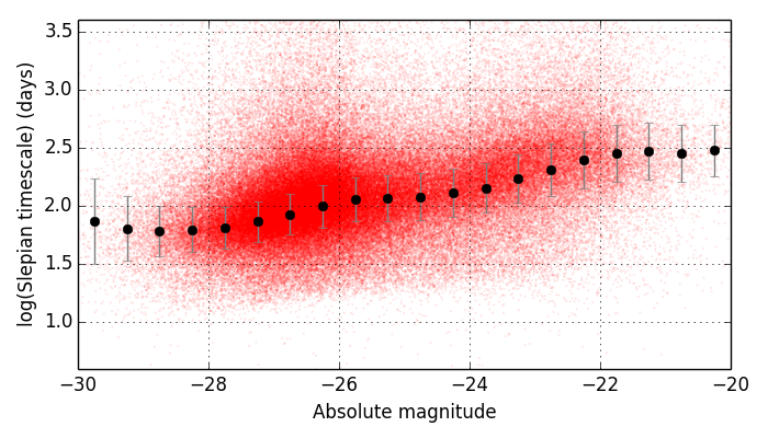
Figure 1: The characteristic restframe timescale determined from the Slepian wavelet variance as a function of absolute magnitude for the 243,500 quasars in the data set. The black points indicate the median value in each magnitude bin.

2.2 Autocorrelation function (ACF)

The autocorrelation function (ACF) is a measure of how closely a quantity observed at a given time is related to the same quantity at another time (the time difference between the two is the lag time). In the case of a (quasi-)periodic signal, peaks in the ACF will indicate lag times at which the signal is perfectly (highly) correlated with itself and these can be interpreted as periods at which the signal (quasi-)repeats. The peak at zero lag $(\tau=0)$ is the strongest peak in the ACF of a (quasi-)periodic signal. Successive peaks at increasing multiples of the period are increasingly weaker, and as the lag value approaches the coherence time – the time required for a signal to change its frequency and phase information, the peaks in the autocorrelation function approach the “noise floor” generated by the non-periodic components of the signal and the noise.

McQuillan et al. (2013) discuss the robustness of the ACF for period detection in time series data. Since the ACF measures only the degree of self-similarity of the light curve at a given lag time, the period remains detectable even when the amplitude and phase of the photometric modulation evolve significantly during the timespan of the observations. The ACF is also not susceptible to residual instrumental systematics since correlated noise, long-term trends and discontinuities manifest as monotonic trends in the ACF, on top of which local maxima may still be identified. In fact, the ACF is preferable as a period-finding method to the Lomb-Scargle periodogram in terms of clarity and robustness.

For irregularly sampled data, the standard ACF estimator of Edelson & Krolik (1988) can be defined as:

$$ACF(k\Delta\tau)=\frac{\sum_{i=1}^{n}\sum_{j>i}x_{i}x_{j}b_{k}(t_{j}-t_{i})}{\sum_{i=1}^{n}\sum_{j=1}^{n}b_{k}(t_{j}-t_{i})}$$

where the observations have been normalized to zero mean and unit variance before the analysis. The kernel $b_{k}(t_{j}-t_{i})$ selects the observations whose time lag is not further than half the bin width from $k\Delta\tau$:

$$b_{k}(t_{j}-t_{i}) = 1\,\,\mathrm{for}\mid(t_{j}-t_{i})/\Delta\tau-k\mid\,\,<1/2$$

$$0\,\,\mathrm{otherwise}$$

However, this estimator has a number of disadvantages including a high variance and not always producing positive semidefinite covariance matrix estimates (necessary to ensure the non-negativity of its Fourier transform; Rehfeld et al. 2011 ). Whilst a Gaussian kernel addresses some of these, Alexander (2013) recommends Fisher’s $z$-transform and equal population binning (at least 11 points in each $\Delta\tau$ bin) for a more effective estimator. Fig. 2 shows the ACF for a sample quasar light curve calculated using both the z-transform method and Scargle’s alternative method (Scargle, 1989).

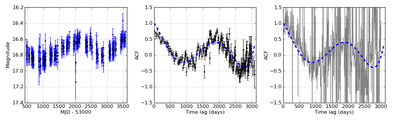
Figure 2: The autocorrelation function for the given quasar light curve (left) evaluated using the $z$-transform method (middle) and Scargle’s method (right). The dashed line shows the best-fit polynomial for the $z$-transform fit constrained to go through ACF(0) = 1.

McQuillan et al. (2013) identify the rotation periods of Kepler field M-dwarfs from the largest peaks (relative to neighbouring local minima) in their ACFs smoothed with a fixed width Gaussian kernel. Our data, however, have variable sampling in terms of cadence, temporal baseline and number of observations, which makes defining a single smoothing width value difficult. We have found that a better procedure to determine the period of any signal in the data is to fit the ACF of a light curve with a Gaussian process model (also known as kriging). Assuming the process has a squared-exponential covariance, this provides the best linear unbiased prediction of the underlying function from noisy data. We define the period as the time-lag value associated with the largest peak in the ACF between the second and third zero-crossings of the fitted model. This shows very good agreement with values determined from ACFs smoothed with a range of different width Gaussian kernels. We have verified the period determined by this method with that obtained with the conditional entropy algorithm of Graham et al. (2013). We would expect broad agreement between the period determined from the ACF and that identified by the wavelet technique.

Periodically driven stochastic systems are expected to have an ACF with the form of an exponentially decaying cosine function (Jung, 1993). Alternatively, if the light curve is the result of a continuous autoregressive moving average CARMA process (CARMA) (see Sec. 6.1) then its ACF is a sum of exponentially damped sinusoids and exponential decays, depending on whether the roots of the characteristic polynomial of the CARMA process are real or imaginary (Kelly et al. 2014, ). To test either case, we have also determined the best fitting exponentially damped sinusoid to the ACF of the form: $ACF(\tau)=A\cos(\omega\tau)\exp(-\lambda\tau)$, where the amplitude $A$, period $p=2\pi/\omega$, and decay $\lambda$ are determined using maximum likelihood estimation.

2.3 Shape and coverage

In the simplest case, periodicity associated with a Keplerian orbit would show as a pure sinusoidal signal in the light curve. Although the projective geometry of a system – orbital inclination, eccentricity and argument of periastron – will distort this, the variation will remain a smooth periodic function, essentially a multiharmonic sine function. Regular flaring activity and similar phenomena not necessarily associated with a close SMBH binary pair would show as (quasi-)periodic discontinuities. We can therefore use the scatter around an expected sinusoidal waveform to identify those objects most closely exhibiting the desired behavior.

The best-fit truncated Fourier series (up to 6 terms) is determined for a given light curve phased using the period calculated by the ACF method (see above):

$$\phi(t)=m_{0}+\sum_{n=1}^{6}a_{n}sin(n\omega t+\phi_{n})$$

where $\phi(t)$ is the phased light curve, $m_{0}$ is the median magnitude and $\omega=2\pi/period_{ACF}$. An F-test is used to determine the exact number of harmonics to include. The scatter about the best fit will be a combination of the intrinsic variability of the quasar and the quality of the fit. We therefore scale the rms scatter of the phased data about the fit by the median absolute deviation (MAD) of the light curve and only consider objects with scatter below some cutoff value as binary candidates. We note, however, that the MAD is a function of magnitude: fainter objects show large MAD values as there is a larger noise contribution for low S/N (faint) sources (see Fig. 3). We therefore employ a MAD value normalized by the median value for a given magnitude to ensure that objects with equivalent variability strength (irrespective of magnitude) can be compared.

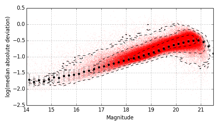
Figure 3: The median absolute deviation - magnitude relationship for the 243,500 quasars in the data set. The black points indicate the median value in each magnitude bin. The contours indicate the 1$\sigma$, 2$\sigma$ and 3$\sigma$ levels.

The temporal coverage of the data set used will determine the range of SMBH masses and binary separations to which it is sensitive (see Fig. 4). A decade-long baseline will only sample a fraction of an orbital period for either a low mass SMBH pair (where the primary BH mass $<10^{7}M_{\odot}$) or a more massive pair at separations $>1$pc. Since we want objects with well-sampled periodic behavior, we limit our search to objects with coverage of at least 1.5 cycles, assuming their ACF determined period. We also only consider objects with more than 50 observations in their light curves to minimize any systematic effects in the statistics from poor sampling.

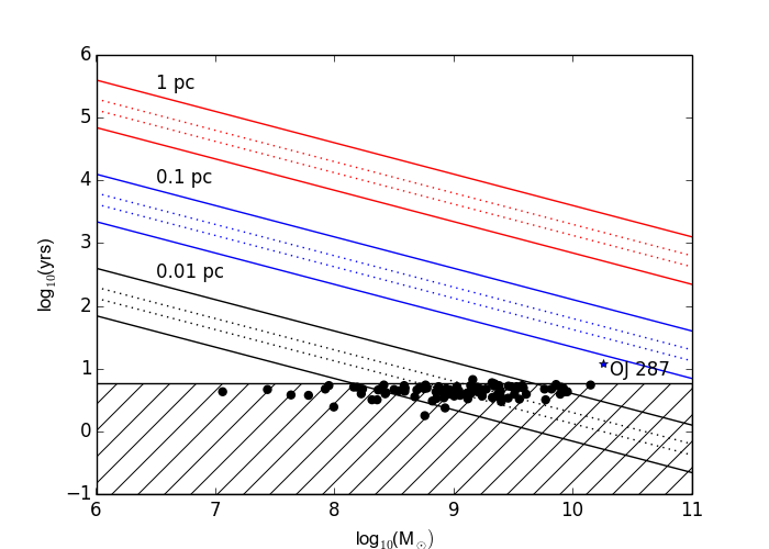
Figure 4: The range of SMBH masses and binary separations to which a synoptic data set is sensitive. The solid upper line for each separation indicates a $z=5$ track and the solid lower line a $z=0.05$ track whilst the two internal dotted lines show $z=1.0$ (lower) and $z=2.0$ (upper) tracks respectively. The hatched region indicates the range over which CRTS has temporal coverage of 1.5 cycles or more of a periodic signal. The points indicate the locations of the CRTS candidates and the best known SMBH binary candidate, OJ 287 (solid black star).

3 Data sets

There are few data sets with sufficient sky and/or temporal coverage and sampling to support an extensive search for quasars exhibiting periodic behavior. Most large studies of long-term quasar variability, e.g., SDSS with POSS (MacLeod et al., 2012) or Pan-STARRS1 (Morganson et al., 2014), consist of relatively few epochs of data spread over a roughly decadal baseline, which is sufficient to model ensemble behavior but not to identify specific patterns in individual objects. CRTS represents the best data currently available with which to systematically define sets of quasars with particular temporal characteristics.

3.1 Catalina Real-time Transient Survey (CRTS)

CRTS leverages the Catalina Sky Survey data streams from three telescopes – the 0.7 m Catalina Sky Survey Schmidt and 1.5 m Mount Lemmon Survey telescopes in Arizona and the 0.5 m Siding Springs Survey Schmidt in Australia – used in a search for Near-Earth Objects, operated by Lunar and Planetary Laboratory at University of Arizona. CRTS covers up to $\sim$2500 deg² per night, with 4 exposures per visit, separated by 10 min, over 21 nights per lunation. All data are automatically processed in real-time, and optical transients are immediately distributed using a variety of electronic mechanisms. The data are broadly calibrated to Johnson $V$ (see Drake et al. 2013 for details) and the full CRTS data set contains time series for approximately 500 million sources.

The Million Quasars (MQ) catalogue v3.7 contains all spectroscopically confirmed type 1 QSOs (309,525), AGN (21,728) and BL Lacs (1,573) in the literature up to 2013 November 26 and formed the basis for the results of Graham et al. (2015). We have extended this with 297,301 spectroscopically identified quasars in the SDSS Data Release 12 (Paris et al., 2015). We crossmatched this combined quasar list against the CRTS data set with a 3″  matching radius and find that 334,446 confirmed quasars are covered by the full CRTS. Of these, 83,782 do not pass our sampling criterion (i.e., they have less than 50 observations in their light curves), leaving a data set of 250,664 quasars. Note that the majority of rejected objects are faint ($V>20$). The magnitude and redshift distributions for our sample are shown in Figs. 5 and 6.

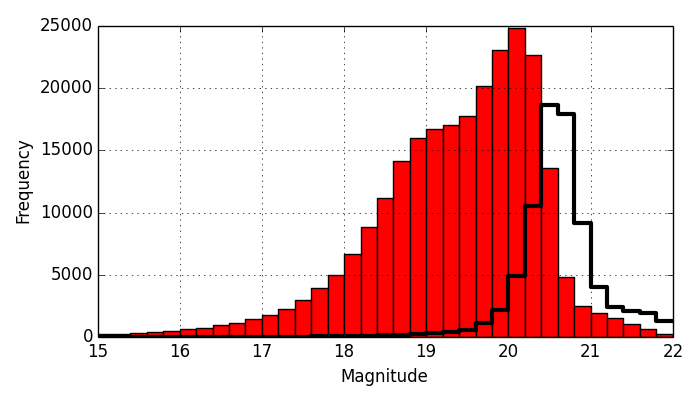
Figure 5: The $V$-band magnitude distribution for the CRTS known quasar sample (red). The tail of sources fainter than $V\sim 20.3$ are from the Mount Lemmon 1.5m telescope in the Catalina surveys. The stepped distribution (black) shows the rejected objects (less than 50 data points) from the sample which are primarily fainter sources.

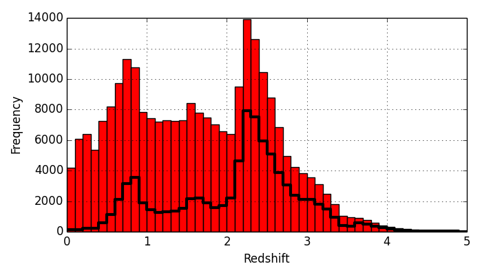
Figure 6: The redshift distribution for the CRTS known quasar sample (red), omitting the tail of the distribution which contains 164 quasars with $z>5.$ The stepped distribution (black) again shows the rejected objects.

3.2 Preprocessing

It is common to preprocess data to remove spurious outlier points which may be caused by technical or photometric error. The danger, of course, is removing real signal, although a robust method should be unaffected by the presence of noisy data. We have created a cleaned version of each data set following the procedure of Palanque-Delabrouille et al. (2011) (PD11): a 3-point median filter was first applied to each time series, followed by a clipping of all points that still deviated significantly from a quintic polynomial fit to the data. To ensure that not too many points are removed, the clipping threshold was initially set to 0.25 mag and then iteratively increased (if necessary) until no more than 10% of the points were rejected. Note that PD11 used a 5$\sigma$ threshold but we found that this removed too few points and so used the limit set by Schmidt et al. (2010) instead.

There is always a chance that the light curve for a particular object may be contaminated by stray light (e.g., diffraction spikes, reflections) from nearby bright sources (up to $\sim$2′  away for CRTS), low surface brightness galaxies or genuine blends, which can give a false seeing-dependent result in the analysis. If an object has a nearby counterpart (within $\sim$5″) which is unresolved by CRTS ($\sim$2 pixels), the light curve will be the combined signal from both, dominated by the brighter of the two. We have defined a distance and magnitude-based criterion to exclude quasars near bright stars by crossmatching the quasar list against the Tycho catalog of bright stars $(V<14)$ and reject 5,319 sources. We reject all objects within a $350^{\prime\prime}$ radius of any star brighter than $V=6.67$ and within a radius of $200^{\prime\prime}/(V-6)$ for $V>6.67$. To identify blends, we crossmatched our list against SDSS and flagged those objects where there is a significant difference (taking into account the variability of the source) between the magnitude of the CRTS source and the SDSS $r$ of its match, typically indicating a faint close SDSS companion contributing to the CRTS photometry: $|V-r|>5\sigma_{V}$. We also flagged those CRTS quasars outside the SDSS footprint (or without a SDSS companion) where the distribution of the spatial positions of individual photometry points in the light curve show significant scatter, e.g., a bimodal distribution indicating two sources: $\sigma_{pos}>5\sigma_{p}os(V)$ where $\sigma_{p}os(V)$ is the expected positional scatter for all quasar of magnitude $V$. Together these reject another 4.560 sources. The final size of the data set is 243.486 quasars.

3.3 Mock data

To first approximation, quasar variability is well-described by a Gaussian first-order continuous autoregressive model (CAR(1)), also known as a damped random walk or Ornstein-Uhlenbeck process (see Graham et al. 2014 ; Kelly et al. 2014 for details of where this description breaks down). Formally, the temporal behavior of the quasar flux $X(t)$ is given by:

$$dX(t)=-\frac{1}{\tau}X(t)dt+\sigma\sqrt{dt}\epsilon(t)+bdt,\tau,\sigma,t>0$$

where $\tau$ is the relaxation time of the process, $\sigma$ is the variability of the time series on timescales short compared to $\tau$, $b\tau$ is the mean magnitude, and $\epsilon(t)$ is a white noise process with zero mean and variance equal to 1. For each quasar in our data set, we have generated a simulated light curve assuming that it follows a CAR(1) model. Using the actual observation times, $t_{i}$, we replace the observed magnitudes with those that would be expected under a CAR(1) model. The magnitude $X(t)$ at a given timestep $\Delta t$ from a previous value $X(t-\Delta t)$ is drawn from a Gaussian distribution with mean and variance given by, e.g., (Kelly et al., 2009):

$$E(X(t)|X(t-\Delta t))=e^{-\Delta t/\tau}X(t-\Delta t)+b\tau(1-e^{-\Delta t/\tau})$$

$$\mathrm{Var}(X(t)|X(t-\Delta t))=\frac{\tau\sigma^{2}}{2}[1-e^{-2\Delta t/\tau}]$$

We add a Gaussian deviate normalized by the photometric error associated with the magnitude to be replaced at each time $t$ to incorporate measurement uncertainties into the mock light curves. For each light curve, we set $b\tau$ to its median value and use the rest frame CAR(1) fitting functions determined by MacLeod et al. (2010):

$$\log f=A+B\log\left(\frac{\lambda_{RF}}{4000{\mathrm{\AA}}}\right)+C(M_{i}+23)+D\log\left(\frac{M_{BH}}{10^{9}M_{\odot}}\right)$$

where $(A,B,C,D)=(-0.51,-0.479,0.131,0.18)$ for $f=SF_{\infty}$ and $(A,B,C,D)=(2.4,0.17,0.03,0.21)$ for $f=\tau$. Note that a value of $C=0.113$ is used for $f=SF_{\infty}$ for non K-corrected magnitudes. $M_{i}$ is the absolute magnitude of the quasar and $\lambda_{RF}$ is the restframe wavelength of the filter – here taken to be SDSS $r$, $\lambda_{RF}=6250{\mathrm{\AA}}/(1+z)$. The mass of the black hole given the absolute magnitude is drawn from a Gaussian distribution:

$$p(\log M_{BH}|M_{i})=\frac{1}{\sqrt{2\pi}\sigma}\exp\left[-\frac{(\log M_{BH}-\mu)^{2}}{2\sigma^{2}}\right]$$

where $\mu=2.0-0.27M_{i}$ and $\sigma=0.58+0.011M_{i}$. This is based on Shen et al. (2008) results. Differences in cosmologies used in estimating the best-fit parameters for CAR(1) and black hole mass should only have a 1% effect (MacLeod thesis, 2012).

4 Results

We have applied our technique which identifies strong periodic behavior to both the real CRTS quasar data set and its simulated counterpart. From the real data set, we define an initial candidate sample according to the following criteria (see Table 1 for a summary). For the wavelet component, we set the decay constant $c=0.001$ and use the frequency range 0.0003 – 0.05 day^-1. As we are interested in well-defined periodicity, we only consider those objects whose wavelet peak significance places them in the top quartile of the data set (in terms of significance), which translates to a WWZ peak value cutoff of $wwzpk>50$. We also only consider objects with a characteristic timescale from their Slepian wavelet variance at least $1\sigma$ below the expected value for their absolute magnitude. This reflects that periodic objects are not expected to be well-described by a CAR(1) model.

Table 1: The selection constraints used to define an initial sample of binary candidates and the respective counts for the real and simulated data sets for each constraint.

Component	Constraint	Real	Mock
Wavelet peak value	$wwzpk>50$	24437	32078
Slepian wavelet deviation	$\tau_{slep}<\tau(M_{V})-\sigma_{\tau}$	37828	27746
WWZ-ACF period	$0.9<p_{ACF}/p_{WWZ}<1.1$	30330	63637
ACF amplitude	$A>0.3$	108625	143447
ACF decay	$\lambda<10^{-3}$	172049	182592
Shape	$rms/MAD<0.67$	11794	3944
Temporal coverage	$\tau/p_{ACF}>1.5$	245234	182257
Number of points	$n>50$	243486	243486
Combined	-	101	0
Final	-	111	0

The first ACF-based constraint is that the periods determined by the WWZ and the ACF, respectively, should agree to within 10 per cent. The shape of the ACF should also be reasonably described by an exponentially damped cosine with not too small an amplitude $(A>0.3)$ and a decay constant such that the ACF drops by at most a factor of $1/e$ over the temporal baseline of the time series. This corresponds to $\lambda<10^{-3}$ for the shortest time coverage in the data set and so we use this as a fiducial value.

In terms of the shape constraint, we limit the selection to those objects whose rms scatter about the best-fit truncated Fourier series to their phased light curve is less than the $1\sigma$ lower limit on the magnitude-normalized median absolute deviation, i.e., $rms/mad<0.67$. Finally, as previously described, we also limit the allowed temporal coverage to 1.5 cycles or greater, i.e. $\tau/period_{ACF}>1.5$, where $\tau$ is the timespan of a light curve, and only consider light curves with 50 or more observations.

Ideally, we want to determine the discriminating hyperplane in the multidimensional feature space that provides a clear separation between periodic and non-periodic objects. The feature cuts that we have defined provide a first approximation to this but likely candidates close to a selection value may have been missed due to error, poor sampling, etc. We therefore use the initial sample defined by the feature cuts as part of the training set for a support vector machine (SVM) with a radial basis function kernel. A number of similar machine learning algorithms could also be employed here but we found from simulations that the SVM was the best in terms of speed and accuracy.

The other part of the training set comprises a set of randomly selected quasars that do not meet the periodicity selection criteria. From simulations with known numbers of periodic objects and periodic/non-periodic ratios, we have determined that the most adequate training set mix is $\sim$100:1, given our expected detection rate (see Section 6.3). 10000 randomly selected “non-periodic” quasars are thus added to the training set. The trained SVM is then used to classify each quasar in the full data set as periodic or not periodic based on their feature values. We repeat this process 50 times and identify those objects in the full data set that are selected each time as periodic as a final binary candidate.

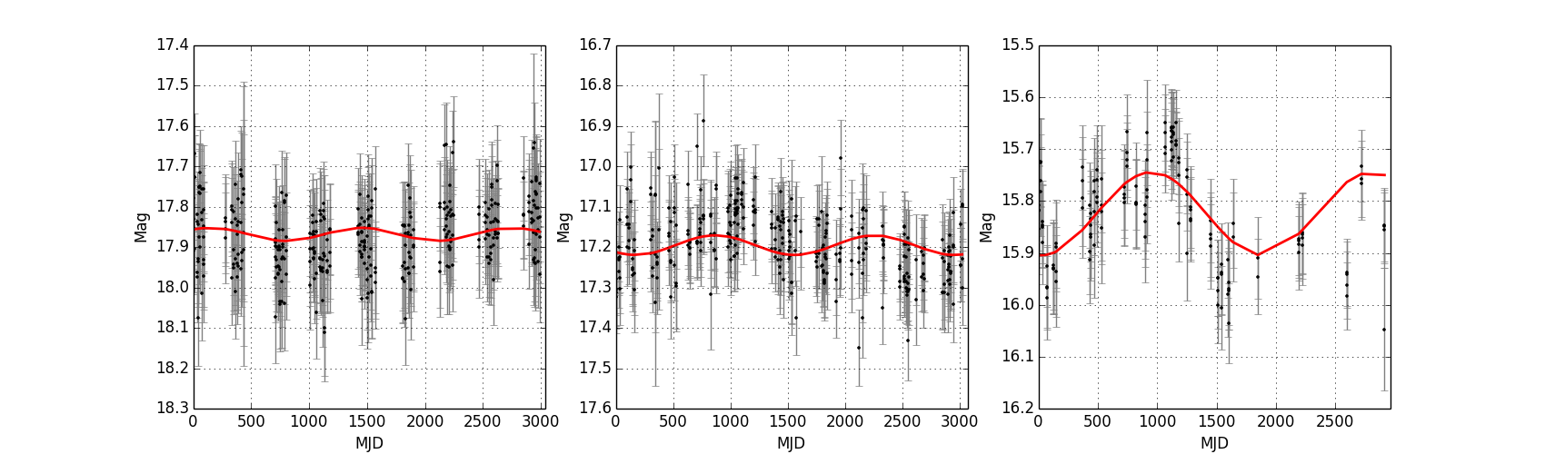
Figure 7: The three objects in the simulated data which most closely match the selection criterion. The best-fit sinusoid for the determined period for each source is plotted in red.

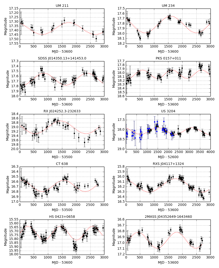
Figure 8: Light curves for periodic candidates. CRTS data (black) is shown; complementary data (blue) from the LINEAR survey (Sesar et al., 2011) is also included where available. The best-fit sinusoid for the determined period is plotted in red. The full set is available online.

Our final sample consists of 111 quasars (see Table 2 for details and Fig. 8 for their light curves). We have also applied the same selection process to the simulated data set of objects with CAR(1) model light curves and find that none of them satisfy our criteria. If we apply the SVM trained on the real data to the simulated data set, we also find that that no objects are selected in all iterations as periodic. There are, however, three mock sources which are selected in almost all iterations (see Fig. 7). Though these objects are the closest to our selection criteria, they look qualitatively different from the real sample with no clear periodicity. The range of variability they exhibit is also significantly more than in the real sample: their mock light curves have MAD values two or three times the values seen in the real data.

Table 2: The 111 periodic quasar candidates meeting the selection criteria. The full version is available in electronic form online. Black hole masses are obtained from Shen et al. (2008) and updates or directly from spectra where a value is not available. Binary system parameters - separation $r$, the restframe merger time $(t_{insp})$ and the maximum induced timing residual amplitude $(\Delta t_{GW})$ - all assume $q=0.5$.

Id	RA	Dec	$z$	$V_{median}$	Period	$\log\left(\frac{M_{BH}}{M_{\odot}}\right)$	$r$	$t_{insp}$	$\Delta t_{GW}$
					(days)		(pc)	(yrs)	(ns)
UM 211	00 12 10.9	$-$01 22 07.6	1.998	17.38	1886	-	-	-	-
UM 234	00 23 03.2	+01 15 33.9	0.729	17.82	1818	9.19	0.013	$1.2\times 10^{4}$	3.0
SDSS J014350.13+141453.0	01 43 50.0	+14 14 54.9	1.438	17.68	1538	9.21	0.009	$2.8\times 10^{3}$	2.4
PKS 0157+011	02 00 03.9	+01 25 12.6	1.170	18.04	1052	-	-	-	-
RX J024252.3-232633	02 42 51.9	$-$23 26 34.0	0.680	19.01	1818	-	-	-	-
US 3204	02 49 28.9	+01 09 25.0	0.954	18.09	1666	8.951	0.009	$1.7\times 10^{4}$	1.0
CT 638	03 18 06.5	$-$34 26 37.4	0.265	16.68	1515	-	-	-	-
RXS J04117+1324	04 11 46.9	+13 24 16.5	0.277	16.20	1851	8.16	0.006	$1.4\times 10^{6}$	0.1
HS 0423+0658	04 26 30.2	+07 05 30.3	0.170	15.73	1123	-	-	-	-
2MASS J04352649-1643460	04 35 26.5	$-$16 43 45.7	0.098	16.96	1369	7.78	0.004	$4.1\times 10^{6}$	0.1
SDSS J072908.71+400836.6	07 29 08.6	+40 08 37.0	0.074	16.08	1612	5.71	0.001	$1.9\times 10^{10}$	0.0
SDSS J080237.60+340446.3	08 02 37.6	+34 04 46.6	1.119	18.40	1428	8.96	0.007	$8.8\times 10^{3}$	0.9
SDSS J080648.65+184037.0	08 06 48.6	+18 40 37.3	0.745	20.61	0892	7.99	0.003	$1.7\times 10^{5}$	0.0
SDSS J080809.56+311519.1	08 08 09.5	+31 15 18.9	2.642	18.91	1162	8.36	0.003	$1.2\times 10^{4}$	0.1
SDSS J081133.43+065558.1	08 11 33.4	+06 55 58.3	1.266	18.48	1587	9.39	0.010	$1.8\times 10^{3}$	5.0
SDSS J081617.73+293639.6	08 16 17.8	+29 36 40.7	0.768	17.80	1162	9.77	0.013	$3.6\times 10^{2}$	23.7
FBQS J081740.1+232731	08 17 40.2	+23 27 32.0	0.891	16.58	1190	9.55	0.011	$7.4\times 10^{2}$	9.6
SDSS J082121.88+250817.5	08 21 22.0	+25 08 16.2	1.906	17.74	1886	9.53	0.011	$8.8\times 10^{2}$	8.2
SDSS J082716.85+490534.0	08 27 16.9	+49 05 34.9	0.682	18.38	1612	8.96	0.009	$2.2\times 10^{4}$	1.3
SDSS J082827.84+400333.9	08 28 27.8	+40 03 34.1	0.968	17.79	1886	8.87	0.008	$3.1\times 10^{4}$	0.8
SDSS J082926.01+180020.7	08 29 26.0	+18 00 20.7	0.810	19.81	1449	8.42	0.005	$1.1\times 10^{5}$	0.1
SDSS J083349.55+232809.0	08 33 49.6	+23 28 09.2	1.155	17.58	1086	9.40	0.008	$7.4\times 10^{2}$	4.7
SDSS J084146.19+503601.1	08 41 46.3	+50 36 00.5	0.555	18.49	1694	7.44	0.003	$1.1\times 10^{7}$	0.0
BZQJ0842+4525	08 42 15.3	+45 25 45.0	1.408	17.20	1886	9.48	0.012	$1.7\times 10^{3}$	7.3
SDSS J091554.50+352949.6	09 15 54.5	+35 29 49.9	0.896	17.92	1369	9.05	0.008	$7.3\times 10^{3}$	1.5
SBS 0920+590	09 23 58.7	+58 49 06.3	0.709	16.76	0649	8.76	0.004	$4.1\times 10^{3}$	0.4
SDSS J092911.35+203708.5	09 29 11.3	+20 37 09.2	1.845	18.51	1785	9.92	0.014	$1.8\times 10^{2}$	36.2
HS 0926+3608	09 29 52.1	+35 54 49.6	2.150	16.99	1562	9.95	0.012	$8.4\times 10^{1}$	38.8
SDSS J093819.25+361858.7	09 38 19.3	+36 18 58.9	1.677	18.80	1265	9.32	0.007	$8.3\times 10^{2}$	3.3
SDSS J094450.76+151236.9	09 44 50.7	+15 12 37.5	2.118	17.72	1428	9.61	0.009	$2.6\times 10^{2}$	10.0
SDSS J094715.56+631716.4	09 47 15.6	+63 17 17.3	0.487	16.10	1724	9.22	0.012	$1.3\times 10^{4}$	4.3
HS 0946+4845	09 50 00.7	+48 31 29.9	0.589	16.87	1587	8.59	0.007	$1.0\times 10^{5}$	0.3
KUV 09484+3557	09 51 23.9	+35 42 49.2	0.398	17.77	1162	8.31	0.005	$1.8\times 10^{5}$	0.1
SDSS J102255.21+172155.7	10 22 55.2	+17 21 56.0	1.062	18.48	1666	8.69	0.006	$3.9\times 10^{4}$	0.4
SDSS J102349.38+522151.2	10 23 49.5	+52 21 51.8	0.955	16.96	1785	9.59	0.014	$1.8\times 10^{3}$	12.1
RXS J10304+5516	10 30 25.0	+55 16 23.4	0.435	16.74	1515	8.43	0.006	$2.2\times 10^{5}$	0.2
SDSS J103111.52+491926.5	10 31 11.5	+49 19 27.2	1.203	17.64	1612	9.04	0.008	$7.8\times 10^{3}$	1.3
SDSS J104430.25+051857.2	10 44 30.3	+05 18 56.8	0.905	17.33	1333	9.24	0.009	$3.3\times 10^{3}$	3.0
SDSS J104758.34+284555.8	10 47 58.3	+28 45 56.2	0.792	19.09	1851	8.72	0.008	$6.9\times 10^{4}$	0.5
SDSS J104941.01+085548.4	10 49 41.0	+08 55 48.5	1.185	17.87	1428	9.37	0.009	$1.7\times 10^{3}$	4.5
MS 10548-0335	10 57 22.3	–3 51 31.3	0.555	17.67	0892	-	-	-	-
CSO 67	11 03 27.5	+29 48 11.2	0.909	17.52	2083	9.35	0.013	$7.1\times 10^{3}$	5.2
SDSS J110554.78+322953.7	11 05 54.8	+32 29 54.1	0.151	17.45	1724	8.24	0.007	$1.2\times 10^{6}$	0.2
SDSS J113050.21+261211.4	11 30 50.2	+26 12 11.8	1.012	17.69	2173	9.32	0.013	$7.6\times 10^{3}$	4.6
SDSS J113916.47+254412.6	11 39 16.4	+25 44 13.0	1.012	17.61	2439	9.16	0.012	$1.9\times 10^{4}$	2.6
SDSS J114438.34+262609.4	11 44 38.3	+26 26 10.1	0.974	18.39	1315	9.38	0.010	$1.7\times 10^{3}$	4.9
SDSS J114749.70+163106.7	11 47 49.7	+16 31 06.8	0.554	18.78	1449	8.22	0.005	$3.5\times 10^{5}$	0.1
SDSS J114857.33+160023.1	11 48 57.4	+16 00 22.7	1.224	18.14	1851	9.90	0.017	$4.1\times 10^{2}$	37.6
SDSS J115141.81+142156.6	11 51 41.8	+14 21 57.0	1.002	18.11	1492	9.11	0.009	$6.3\times 10^{3}$	1.8
SDSS J115346.39+241829.4	11 53 46.4	+24 18 29.8	0.753	18.41	1666	8.97	0.009	$2.1\times 10^{4}$	1.3
SDSS J121018.34+015405.9	12 10 18.3	+01 54 06.2	0.216	16.90	1612	8.54	0.008	$2.6\times 10^{5}$	0.6
SDSS J121018.66+185726.0	12 10 18.7	+18 57 27.0	1.516	17.42	1754	9.53	0.011	$1.1\times 10^{3}$	8.4
SDSS J121056.83+231912.5	12 10 56.8	+23 19 13.0	1.260	18.47	1785	8.78	0.007	$2.7\times 10^{4}$	0.5

Table 3: continued

Id	RA	Dec	$z$	$V_{median}$	Period	$\log\left(\frac{M_{BH}}{M_{\odot}}\right)$	$r$	$t_{insp}$	$\Delta t_{GW}$
					(days)		(pc)	(yrs)	(ns)
SDSS J121457.39+132024.3	12 14 57.4	+13 20 24.5	1.494	18.59	1923	9.46	0.011	$1.8\times 10^{3}$	6.6
SDSS J123147.27+101705.3	12 31 47.3	+10 17 05.4	1.733	18.83	1851	9.20	0.009	$3.5\times 10^{3}$	2.3
SDSS J123821.84+030024.2	12 38 21.8	+03 00 24.6	0.380	18.46	1250	8.92	0.008	$2.2\times 10^{4}$	1.4
SDSS J124044.49+231045.8	12 40 44.5	+23 10 46.1	0.722	18.40	1428	8.94	0.008	$1.6\times 10^{4}$	1.1
SDSS J124119.04+203452.7	12 41 19.0	+20 34 53.4	1.492	18.44	1219	9.40	0.008	$6.8\times 10^{2}$	4.5
SDSS J124157.90+130104.1	12 41 57.9	+13 01 04.7	1.227	18.83	1538	8.95	0.007	$9.4\times 10^{3}$	0.9
PGC 3096192	12 50 29.0	+06 36 11.1	0.133	16.93	1562	7.06	0.003	$8.5\times 10^{7}$	0.00
SDSS J125414.23+131348.1	12 54 14.2	+13 13 48.4	0.655	18.11	1754	8.94	0.009	$3.2\times 10^{4}$	1.2
SDSS J130040.62+172758.4	13 00 40.6	+17 27 58.5	0.863	19.26	1818	8.88	0.008	$3.2\times 10^{4}$	0.8
BZQJ1305-1033	13 05 33.0	–10 33 19.1	0.286	14.99	1694	8.50	0.008	$3.0\times 10^{5}$	0.4
SNU J13120+0641	13 12 04.7	+06 41 07.6	0.242	15.82	1492	9.14	0.012	$2.0\times 10^{4}$	5.1
SDSS J131706.19+271416.7	13 17 06.2	+27 14 16.7	2.672	17.83	1666	9.92	0.011	$7.7\times 10^{1}$	33.9
SDSS J131909.08+090814.7	13 19 09.1	+09 08 15.1	0.882	18.01	1298	8.67	0.006	$2.8\times 10^{4}$	0.3
SDSS J132103.41+123748.2	13 21 03.4	+12 37 48.1	0.687	18.62	1538	8.91	0.008	$2.4\times 10^{4}$	1.0
SDSS J133127.31+182416.9	13 31 27.3	+18 24 17.1	0.938	17.44	1639	9.39	0.011	$3.0\times 10^{3}$	5.6
SDSS J133516.17+183341.4	13 35 16.1	+18 33 41.8	1.192	17.75	1724	9.76	0.015	$6.0\times 10^{2}$	21.7
SDSS J133631.45+175613.8	13 36 31.4	+17 56 14.1	0.421	18.20	1562	9.03	0.010	$2.4\times 10^{4}$	2.2
SDSS J133654.44+171040.3	13 36 54.4	+17 10 40.8	1.231	17.96	1408	9.24	0.008	$2.5\times 10^{3}$	2.7
SDSS J133807.69+360220.3	13 38 07.7	+36 02 20.3	1.196	18.44	1960	9.14	0.010	$9.1\times 10^{3}$	2.1
SDSS J134820.42+194831.5	13 48 20.4	+19 48 31.9	0.594	18.34	1388	7.63	0.003	$2.8\times 10^{6}$	0.0
SDSS J134855.27-032141.4	13 48 55.3	–3 21 41.4	2.099	17.19	1428	9.89	0.011	$8.7\times 10^{1}$	30.0
SDSS J135225.80+132853.2	13 52 25.8	+13 28 53.3	0.402	16.44	1754	8.75	0.009	$1.0\times 10^{5}$	0.8
SDSS J140600.26+013252.2	14 06 00.3	+01 32 52.4	0.454	18.00	2000	8.41	0.007	$4.7\times 10^{5}$	0.2
SDSS J140704.43+273556.6	14 07 04.5	+27 35 56.3	2.222	17.32	1562	9.94	0.012	$8.4\times 10^{1}$	36.3
HE 1408-1003	14 10 40.3	–10 17 29.7	0.882	17.01	1923	-	-	-	-
SDSS J141425.92+171811.2	14 14 25.9	+17 18 11.6	0.409	18.33	1785	8.59	0.008	$1.9\times 10^{5}$	0.4
3C 298.0	14 19 08.2	+06 28 35.1	1.437	16.53	1960	9.57	0.013	$1.3\times 10^{3}$	10.5
SDSS J142301.96+101500.1	14 23 02.0	+10 15 00.0	1.052	17.96	1234	9.46	0.010	$9.\times 10^{2}$	6.3
SDSS J143621.29+072720.8	14 36 21.3	+07 27 21.1	0.889	17.07	1886	9.03	0.010	$1.9\times 10^{4}$	1.5
SDSS J143820.60+055447.9	14 38 20.6	+05 54 48.1	0.614	18.71	1851	8.19	0.006	$6.9\times 10^{5}$	0.1
SDSS J144754.62+132610.0	14 47 54.6	+13 26 10.4	0.572	18.39	1960	8.58	0.008	$1.9\times 10^{5}$	0.4
SDSS J144755.57+100040.0	14 47 55.6	+10 00 40.4	0.678	17.65	0862	8.93	0.006	$4.7\times 10^{3}$	0.9
SDSS J150450.16+012215.5	15 04 50.2	+01 22 15.8	0.967	17.75	1724	9.20	0.010	$7.0\times 10^{3}$	2.7
QNZ3:54	15 18 06.6	+01 31 34.9	1.402	18.64	1724	9.27	0.009	$3.1\times 10^{3}$	3.2
SDSS J152035.23+095925.2	15 20 35.2	+09 59 25.7	1.049	18.88	1204	9.12	0.007	$3.3\times 10^{3}$	1.7
SDSS J152157.02+181018.6	15 21 57.0	+18 10 19.2	0.731	18.23	1960	7.95	0.005	$1.6\times 10^{6}$	0.0
SDSS J153636.22+044127.0	15 36 36.2	+04 41 26.9	0.379	16.75	1111	8.82	0.007	$2.4\times 10^{4}$	0.9
SDSS J154409.61+024040.0	15 44 09.6	+02 40 39.8	0.964	18.72	2000	8.76	0.008	$5.5\times 10^{4}$	0.5
SDSS J155449.11+084204.8	15 54 49.1	+08 42 05.4	0.786	17.03	1562	8.85	0.008	$2.6\times 10^{4}$	0.8
SDSS J155647.78+181531.5	15 56 47.8	+18 15 32.1	1.502	18.79	1428	9.51	0.010	$6.7\times 10^{2}$	7.2
SDSS J160730.33+144904.3	16 07 30.3	+14 49 04.2	1.800	17.57	1724	9.82	0.013	$2.5\times 10^{2}$	24.6
SDSS J161013.67+311756.4	16 10 13.7	+31 17 56.6	0.245	17.19	1724	7.92	0.005	$3.2\times 10^{6}$	0.1
SDSS J161854.64+230859.1	16 18 54.6	+23 08 59.3	0.561	18.22	1666	8.37	0.006	$2.9\times 10^{5}$	0.1
163107.34+560905.3	16 31 07.4	+56 09 05.1	0.731	19.13	1724	8.38	0.006	$2.2\times 10^{5}$	0.1
HS 1630+2355	16 33 02.7	+23 49 28.8	0.821	15.23	2040	9.86	0.020	$1.1\times 10^{3}$	38.7
SDSS J164452.71+430752.2	16 44 52.7	+43 07 52.9	1.715	17.06	2000	10.15	0.019	$1.1\times 10^{2}$	91.6
SDSS J165136.76+434741.3	16 51 36.8	+43 47 41.9	1.604	18.13	1923	9.34	0.010	$2.6\times 10^{3}$	4.1
MCG 5-40-026	17 01 07.8	+29 24 24.6	0.036	14.65	1408	-	-	-	-
SDSS J170616.24+370927.0	17 06 16.2	+37 09 27.0	1.267	18.19	1388	9.10	0.007	$3.9\times 10^{3}$	1.6
HS 1715+2131	17 17 20.1	+21 28 15.0	0.590	16.19	1250	-	-	-	-
FBQS J17239+3748	17 23 54.3	+37 48 41.7	0.828	17.55	1960	9.38	0.013	$6.0\times 10^{3}$	6.1
SDSS J172656.96+600348.5	17 26 56.9	+60 03 49.1	0.991	18.50	1923	9.15	0.010	$1.1\times 10^{4}$	2.3
4C 50.43	17 31 03.7	+50 07 35.7	1.111	16.74	1075	-	-	-	-
BZQJ2156-2012	21 56 33.7	–20 12 30.2	1.309	17.01	1333	-	-	-	-
SDSS J221016.97+122213.9	22 10 17.0	+12 22 14.0	0.717	18.32	1333	9.00	0.008	$1.1\times 10^{4}$	1.4
6QZ J221925.1-305408	22 19 25.2	–30 54 08.1	0.579	19.15	1408	-	-	-	-
HS 2219+1944	22 22 21.1	+19 59 48.1	0.211	16.33	1724	-	-	-	-
SDSS J224829.47+144418.0	22 48 29.4	+14 44 18.4	0.424	18.82	1219	8.86	0.008	$2.4\times 10^{4}$	1.0

If we take the simulated data results as an indication of the expected number of quasars to show comparable periodic behavior by chance then the number of real objects selected is statistically significant, particularly with the higher temporal coverage constraint. It also suggests strong periodicity (on an approximately decadal timescale) is not common in quasars nor is it expected as an artifact of a CAR(1) process. We note, however, that our selection criteria will select against longer periodic as well as more general quasi-periodic behavior as may be expected from SMBH binaries at greater than 1 pc separation.

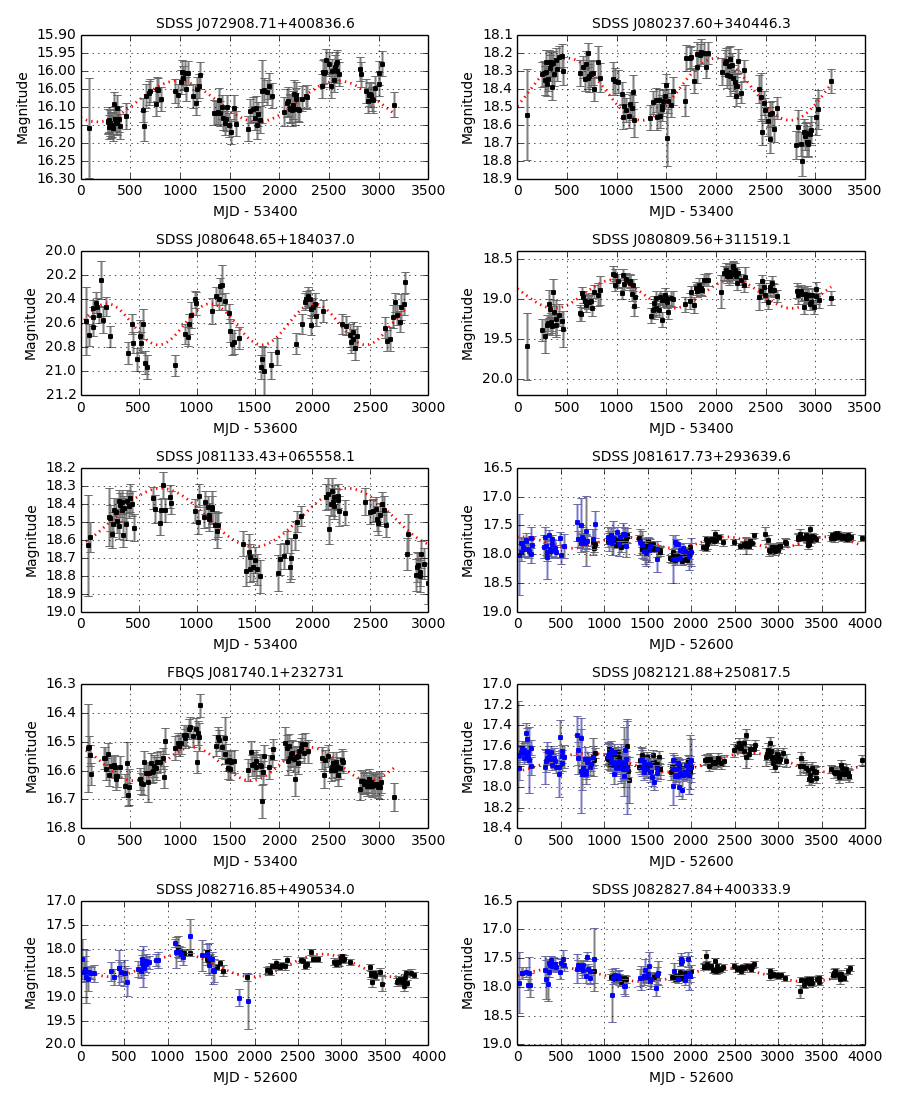
Figure 9: continued

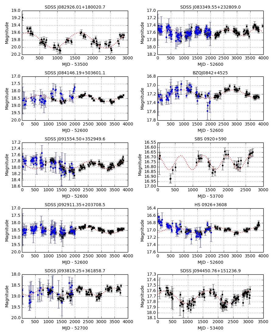
Figure 10: continued

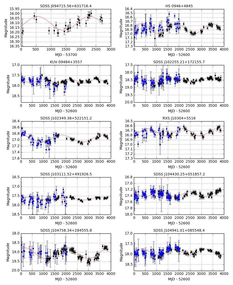
Figure 11: continued

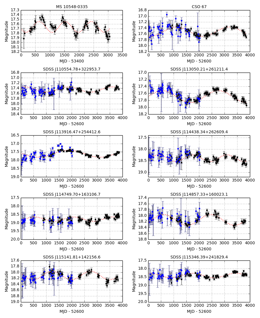
Figure 12: continued

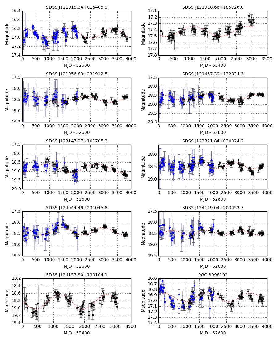
Figure 13: continued

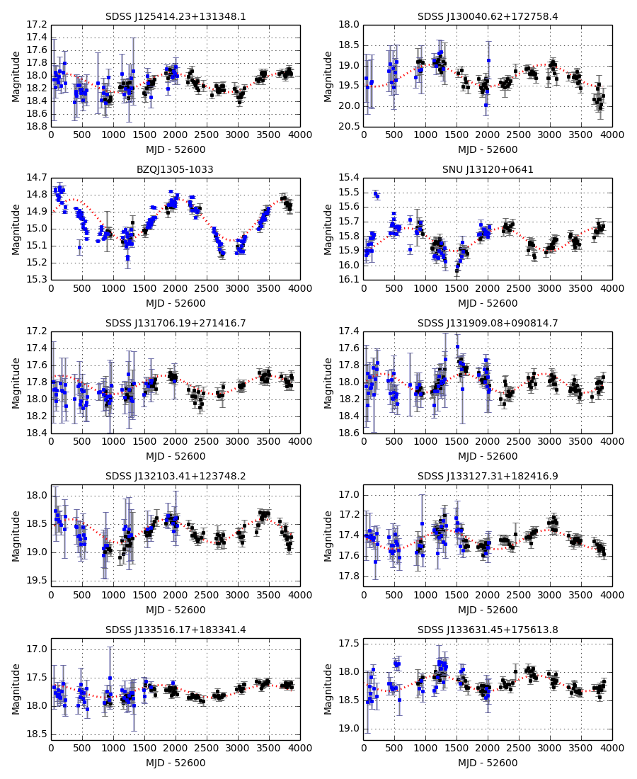
Figure 14: continued

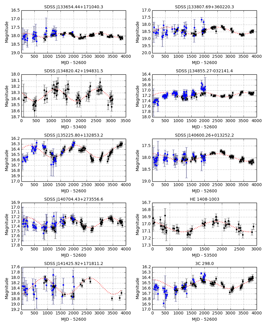
Figure 15: continued

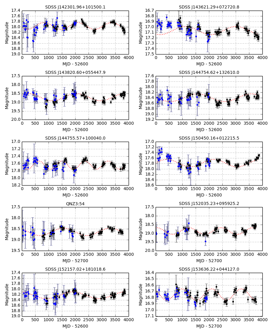
Figure 16: continued

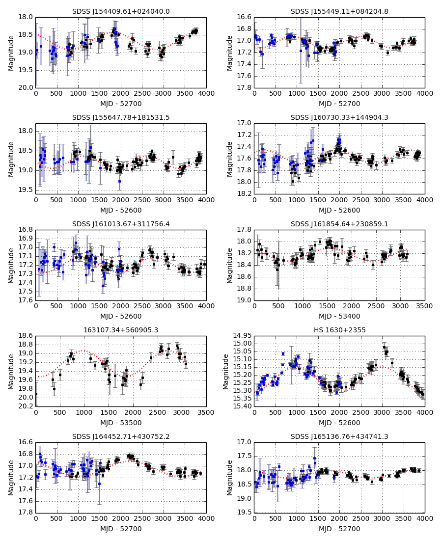
Figure 17: continued

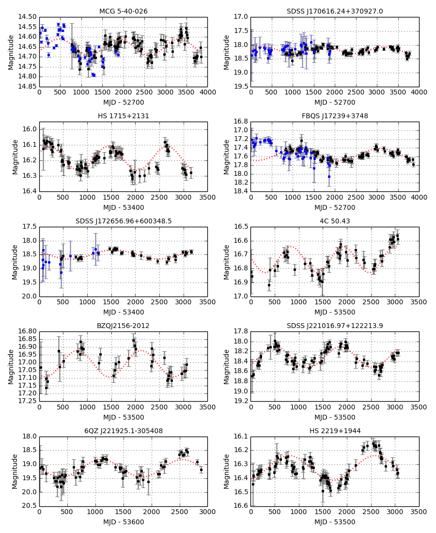
Figure 18: continued

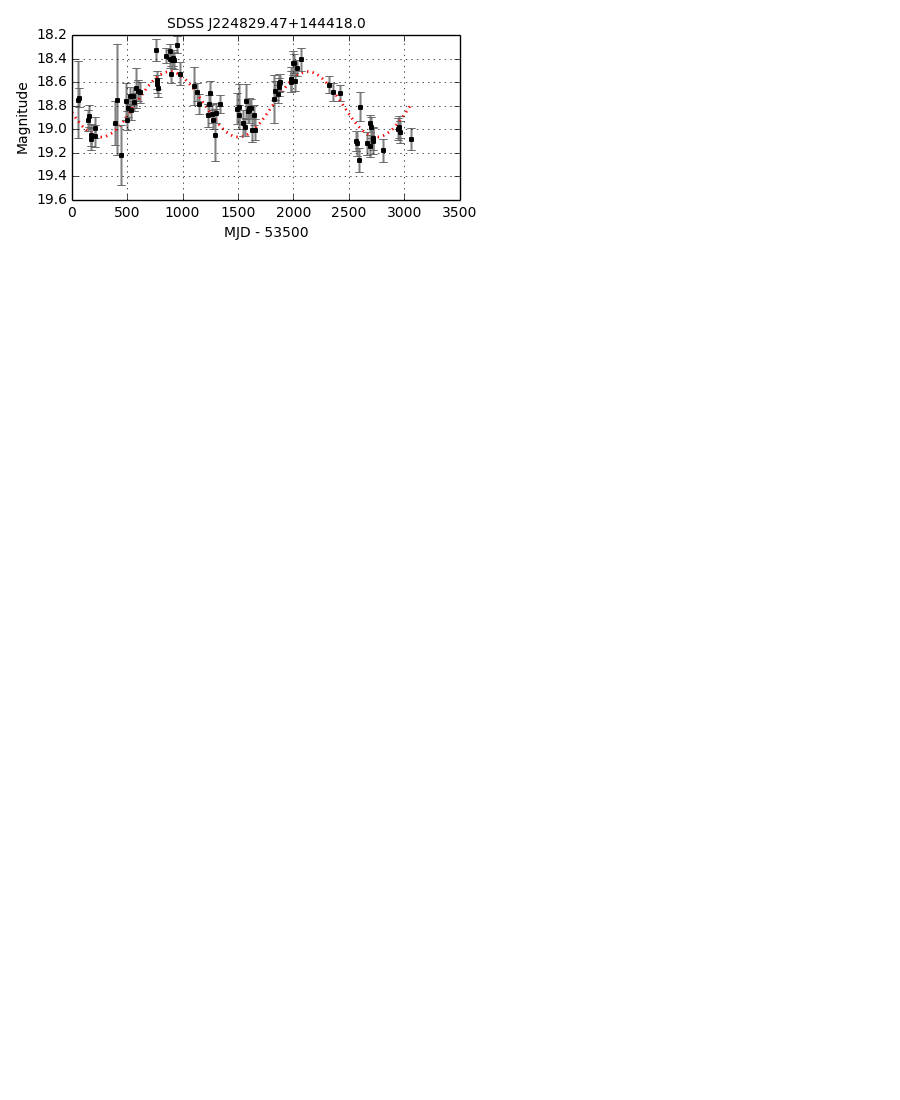
Figure 19: continued

5 Binary Candidates in the Literature

5.1 Spectroscopic

As previously mentioned, the availability of multiepoch spectroscopy enables searches for SMBH binaries on the basis of time-dependent velocity shifts in the broad lines, either with respect to each other or narrow lines associated with the host galaxy. It is interesting to see whether any spectroscopically selected candidates in the literature show periodic photometric variability in CRTS data. We have examined the light curves of 30 spectroscopic SMBH binary candidates from the literature (see Table 4). We only consider here the most likely binary candidates reported, e.g., classified as such from the shape of their Balmer lines (Tsalmantza 2011, ; Decarli et al. 2013, ), and not secondary candidates also reported with asymmetric line profiles, double-peaked emitters, or other features since these do not sufficiently indicate a SMBH binary. Although the predicted separation of these candidates is greater than in our candidates, it is still typically less than 1 pc and we would expect there to be some detectable behavior in the photometric data.

Table 4: SMBH binary candidates identified in the literature

			Best fits
Id	RA	Dec	Shape	Poly	$\log_{10}\tau$	$\log_{10}\sigma^{2}$	CARMA	MAD	Source
J0049+0026	00 49 19.0	+00 26 09.4	Hump	3	2.999	-4.579	(2, 0)	0.10	Optical10
J0301+0004	03 01 00.2	+00 04 29.3	Periodic	1	-1.957	0.753	(4, 0)	0.21	Optical9
J0322+0055	03 22 13.9	+00 55 13.4	Polynomial	5	2.720	-4.327	(6, 0)	0.07	Optical9
J0757+4248	07 57 00.7	+42 48 14.5	Logistic	3	3.235	-5.031	(2, 0)	0.11	Optical10
J0829+2728	08 29 30.6	+27 28 22.7	Polynomial	4	3.095	-3.827	(4, 0)	0.23	Optical8,12
J0847+3732	08 47 16.0	+37 32 18.1	Polynomial	4	2.844	-4.001	(4, 0)	0.12	Optical8
J0852+2004	08 52 37.0	+20 04 11.0	Hump	4	2.594	-3.871	(4, 0)	0.15	Optical8
OJ 287	08 54 48.9	+20 06 30.6	Periodic	5	1.678	-2.021	(7, 0)	0.34	Optical1
J0927+2943	09 27 04.4	+29 44 01.3	Periodic	2	2.882	-4.639	(1, 0)	0.09	Optical2,7,11
J0928+6025	09 28 38.0	+60 25 21.0	Periodic	1	2.650	-4.105	(6, 0)	0.10	Optical8
J0932+0318	09 32 01.6	+03 18 58.7	Polynomial	5	2.921	-4.119	(4, 0)	0.13	Optical6,7,11
J0935+4331	09 35 02.5	+43 31 10.7	Hump	5	2.946	-4.541	(6, 0)	0.05	Optical10
4C 40.24	09 48 55.3	+40 39 44.6	Polynomial	5	2.900	-4.500	(2, 0)	0.09	Radio13
J0956+5350	09 56 56.4	+53 50 23.2	Periodic	1	2.713	-4.392	(4, 0)	0.10	Optical10
J1000+2233	10 00 21.8	+22 33 18.6	Polynomial	7	2.142	-3.593	(7, 0)	0.12	Optical5,7,11
J1012+2613	10 12 26.9	+26 13 27.2	Logistic	2	2.936	-4.557	(5, 0)	0.09	Optical7,11
J1030+3102	10 30 59.1	+31 02 55.8	Hump	3	2.780	-4.134	(5, 0)	0.08	Optical8
J1050+3456	10 50 41.4	+34 56 31.3	Polynomial	10	2.689	-4.154	(2, 0)	0.12	Optical4,7,11
J1100+1709	11 00 51.0	+17 09 34.3	Hump	1	2.906	-4.232	(6, 0)	0.12	Optical8,12
J1112+1813	11 12 30.9	+18 31 11.4	Polynomial	6	2.784	-4.264	(3, 0)	0.09	Optical8
J1154+0134	11 54 49.4	+01 34 43.6	Logistic	1	2.906	-3.853	(5, 2)	0.15	Optical7,11
J1229-0035	12 29 09.5	$-$00 35 30.0	Polynomial	4	2.834	-3.947	(6, 5)	0.13	Optical9
J1229+0203	12 29 06.7	+02 03 08.7	Polynomial	5	1.397	-3.057	(7, 2)	0.07	Radio13
J1305+1819	13 05 34.5	+18 19 32.9	Polynomial	8	2.728	-4.899	(5, 0)	0.04	Optical8,12
J1345+1144	13 45 48.5	+11 44 43.5	Hump	4	2.440	-4.039	(6, 0)	0.08	Optical8
J1410+3643	14 10 20.6	+36 43 22.7	Logistic	3	3.240	-4.434	(5, 0)	0.15	Optical9
J1536+0441	15 36 36.2	+04 41 27.1	Polynomial	10	2.732	-4.474	(6, 0)	0.07	Optical3,7,11
J1537+0055	15 37 06.0	+00 55 22.8	Polynomial	2	3.105	-5.987	(2, 0)	0.03	Optical9
J1539+3333	15 39 08.1	+33 33 27.6	Periodic	1	3.042	-5.591	(2, 0)	0.06	Optical7,11
J1550+0521	15 50 53.2	+05 21 12.1	Hump	1	2.804	-4.817	(2, 0)	0.03	Optical9
J1616+4341	16 16 09.5	+43 41 46.8	Logistic	1	-1.383	-0.033	(4, 0)	0.18	Optical10
J1714+3327	17 14 48.5	+33 27 38.3	Polynomial	7	3.060	-4.865	(1, 0)	0.06	Optical7,11
PKS 2155-304	21 58 52.1	$-$30 13 32.1	Logistic	1	2.483	-2.648	(3, 1)	0.44	Radio13
3C 454.3	22 53 57.7	+16 08 53.6	Polynomial	4	1.978	-1.817	(6, 0)	0.55	Radio13
1ES 2321+419	23 23 52.1	+42 10 59	Polynomial	5	2.531	-2.974	(6, 0)	0.29	X-ray14
J2349-0036	23 49 32.8	$-$00 36 45.8	Periodic	1	-0.337	-1.153	(7, 3)	0.10	Optical9

References: [1] Valtonen et al. (2008); [2] Dotti et al. (2009); [3] Boroson & Lauer 2009; [4] Shields, Bonning & Salviander (2009) ; [5] Decarli et al. (2010); [6] Barrows et al. (2011); [7] Tsalmantza et al. (2011); [8] Liu et al. (2014); [9] Shen et al. (2013); [10] Ju et al. (2013); [11] Decarli et al. 2013 ; [12] Eracleous et al. (2012); [13] Ciaramella et al. (2004); [14] Rani et al. (2009)

There seem to be a number of morphologically distinct behaviors seen with these candidates. To quantify this, we have defined a number of template functions that capture different shape profiles:

Linear: a line with gradient given by the Theil-Sen estimator for the light curve which passes through the median data point $(t_{med},m_{med})$;

Polynomial: the best fitting polynomial up to 10^th order determined by a F-test between successive orders;

Sinusoidal: the best fitting sinusoid with period determined by the ACF method (see section 2.2);

Logistic: a generalized logistic function fit to the light curve:

$$m(t)=A+\frac{K-A}{(1+Qe^{-B(t-M)})^{1/\nu}}$$

Hump/Dip: a linear least-squares fit to the light curve plus a quadratic to the largest contiguous amount of data above or below the linear fit.

For each light curve of interest, we have determined which template function provides the best chi-squared fit. The shape of the light curve may also just be a random pattern arising from the stochastic nature of the variability and so we have also determined both the best-fit CAR(1) and CARMA(p,q) model parameters for each light curve and checked for correlations between these and the best-fitting template. We note that none of the spectroscopic candidates shows the type of strong periodicity exhibited by the candidates identified in this paper.

The division of template shapes is fairly uniform, although objects from Liu et al. (2014) tend to be best-fit by the hump template. These candidates specifically show significant radial accelerations in their broad H$\beta$ lines from dual epoch spectroscopy whereas other studies are based on more or other lines. There is also some suggestion of preferential localization in the CAR(1) $\tau-\sigma^{2}$ plane with objects best fit by a sinusoid function lying outside the $1\sigma$ contour. Those best fit by CARMA models with $p=7$ also show the same effect but to a higher degree. However, the sample size here is too small to determine whether these effects are statistically significant but they certainly warrant further study.

Liu, Shuo & Komossa (2014) proposed SDSS J120136.02+300305.5 as the first milliparsec SMBH binary in a quiescent galaxy on the basis of a candidate tidal disruption event in its X-ray light curve. Its optical light curve shows no significant variation – it has a MAD value of 0.07 mag which is the median value for its magnitude – or evidence of an associated flare and there is no structure to it. This suggests that this population of SMBH binaries will only be detected in the optical as a result of serendipity (assuming that the candidate is an actual binary).

5.2 Blazars

Similarly we have examined the CRTS light curves of the few blazars reported in the literature as exhibiting (quasi-)periodic behavior, e.g., PKS 2155-304 and 1ES 2321+419 (Rani, Wiita & Gupta, 2009). We note that these do not show the consistent periodicity that we see in the candidates in this analysis. However, their CAR(1) and CARMA fits are comparable with those seen for optical candidates in the literature as in the previous section.

5.3 Photometric

Liu et al. (2015) report the discovery of a periodic quasar candidate, FBQS J221648.7+012427, out of a sample of 168 quasars in the Pan-STARRS1 Medium Deep Survey (PSMDS) with an average of 350 detections in four filters. It has an observed period of 542 days, a redshift of 2.06, and an inferred separation of 0.006 pc. Whilst this object is part of the data we have considered, it does not appear as a candidate in our analysis. Assuming the quoted period, its CRTS light curve covers 5.8 cycles but no significant or consistent periodic signal is identified by either the WWZ or ACF algorithms and its Slepian wavelet characteristic timescale is not a statistically significant outlier.

The candidate was identified using a Lomb-Scargle (LS) periodogram to look for evidence of periodicity. A similar approach was used by MacLeod et al. (2010) in a search of 8863 SDSS Stripe 82 quasar light curves (with an average of over 60 observations) with 88 candidates identified. None were considered significant, however, as the standard likelihood calculation assumes white noise as the null hypothesis rather than colored noise as appropriate for an underlying CAR(1) process. The technique is regarded as not very powerful for poorly sampled light curves. It is also interesting to note that both analyses have a detection rate of about 1 in 100 rather than the far more conservative 1 in 10000 that we find, which is much more in line with expected rates from population models (see section 6.3).

The PSMDS candidate FBQS J221648.7+012427 is also reported to have a (restframe) inspiral time of $\sim$ 7 years thus putting its final coalescence within the timeframe of pulsar timing array experiments within the next decade or so. Given that the merger timescale is typically 10⁷ years, it seems statistically unlikely that an object would be found in its final phase in such a small sample size. The inspiral time is, however, very dependent on the black hole mass and so it is possible that the authors have overestimated the mass of the system, particularly as the line and continuum fluxes were not determined from an electronic format spectrum.

6 Discussion

6.1 Quasiperiodic behavior in stochastic models

Although CAR(1) models have been used as popular statistical descriptors of quasar optical variability, e.g., Kelly et al. (2009); MacLeod et al. (2012), there is a growing body of evidence that a more sophisticated approach is required (Mushotzky et al., 2011; Zu et al., 2013; Graham et al. 2014, ; Kasliwal, Vogeley & Richards, 2015). Kelly et al. 2014 describe the use of CARMA models as a better method to quantify stochastic variability in a light curve. (Note that a CAR(1) model is the same as a CARMA(1, 0) model). A zero-mean CARMA(p,q) process $y(t)$ is defined to be the solution to the stochastic differential equation:

$$\frac{d^{p}y(t)}{dt^{p}}+\alpha_{p-1}\frac{d^{p-1}y(t)}{dt^{p-1}}+\ldots+\alpha_{0}y(t)=$$

$$\beta_{q}\frac{d^{q}\epsilon(t)}{dt^{q}}+\beta_{q-1}\frac{d^{q-1}\epsilon(t)}{dt^{q-1}}+\ldots+\epsilon(t)$$

where $\epsilon(t)$ is a continuous time white noise process with zero mean and variance $\sigma^{2}$. This is associated with a characteristic polynomial:

$$A(z)=\sum_{k=0}^{p}\alpha_{k}z^{k}$$

with roots $r_{1},\ldots,r_{p}$. The power spectral density (PSD) for a CARMA(p, q) process is given by:

$$P(\omega)=\sigma^{2}\frac{\mid\sum_{j=0}^{q}\beta_{j}(i\omega)^{j}\mid^{2}}{\mid\sum_{k=0}^{p}\alpha_{k}(i\omega)^{k}\mid^{2}}$$

Now $A(z)$ can be written in terms of its roots:

$$A(z)=\prod_{j=1}^{p}(z-r_{j})=0$$

where $r=a+ib$ and so the PSD is proportional to:

$$P(\omega)\propto\frac{1}{\prod_{j=1}^{p}a_{j}^{2}+(w-b_{j})^{2}}$$

For complex roots (and $p>1$), local maxima will exist at $w=b_{j}$ which correspond to quasi-periodicities in the data. If the roots have negative real parts and $q<p$ then the CARMA process is stationary. By analogy with underdamped second order systems, the quasi-periodicities can be characterized by the damping ratio, $\zeta_{j}=-a_{j}/\sqrt{a_{j}^{2}+b_{j}^{2}}$, for a given frequency, $b_{j}$. Smaller values of $\zeta$ indicate a stronger oscillating signal (less damping) with $\zeta=0$ defining a pure sinusoidal signal. The bandwidth of the signal, i.e., the range of frequencies associated with it, is given by $\Delta f=\zeta b/\pi$.

For each of our periodic candidates, we have determined the best-fitting CARMA(p,q) model using the carma_pack code of Kelly et al. 2014 and checked whether there is any quasi-periodic behavior expected at its identified period from peaks in the PSD. Out of the 111 candidates, we find that five show a detected periodicity which overlaps with that expected from its best-fit CARMA model. However, the bandwidth of all of these is such that any period within the temporal baseline of the object would fit. None of the periodic behavior is therefore consistent with that potentially expected from stochastic variability.

We have also generated 100 mock light curves of the appropriate CARMA(p,q) type for each periodic candidate with the same time sampling as the CRTS data and determined the expected wavelet and ACF parameters. The median differences between the real value and CARMA model-based values are statistically significant in all cases. From this we conclude that CARMA(p,q) models do not provide an adequate statistical description for our periodic candidates as they cannot reproduce the same range of features values seen.

6.2 Physical interpretation

Although we have searched for optical periodicity in quasars on the assumption that this is associated with a close SMBH binary system, the exact physical mechanism responsible for this behavior is uncertain. The sinusoidal nature of the signal suggests that it is kinematic in origin and there are a number of potential explanations that should be considered.

6.2.1 A jet with a varying viewing angle

The optical flux could be the superposition of thermal emission from the accretion disk and a differential Doppler boosted non-thermal contribution associated with a jet (Rieger, 2004). The observed periodicity would be the result of a periodically varying viewing angle, driven either by the orbital motion of a SMBH binary system, a precessing jet or an internally rotating jet flow. In the latter case, the expected observed period is typically $P_{obs}\lesssim 10$ days for massive quasars and even less for objects with significant bulk Lorentz factors, i.e., blazars. Given the range of values we have identified, this seems an unlikely model.

In a single SMBH system, precession of the jet can arise if the accretion disk is tilted (or warped) with respect to the plane of symmetry (although the origin of the tilt would still need to be accounted for). Using data in the literature, Lu & Zhou (2005) find that the expected precession period for a jet with a single SMBH (Lu & Zhou, 2005) is:

$$\log(\tau_{prec}/\mathrm{yr})\sim 0.48M_{abs}+0.14\log\left(\frac{M}{10^{8}M_{\odot}}\right)+A$$

where $A=15.18-18.86$, depending on the values of constant parameters relating to the viscosity and angular momentum of the SMBH system. For a representative quasar with $M_{abs}=-25$ with a $10^{8}M_{\odot}$ SMBH, this gives a period between $10^{2.2-6.9}$ years which is much longer than the observed periods reported here. We note as well that jets in non-blazar systems are predominantly associated with geometrically thick accretion flows in low-luminosity AGN ($L_{bol}\leq 10^{42}$ erg s^-1) whereas the candidate objects considered here span the range $10^{45}\leq L_{bol}\leq 10^{48}$ erg s^-1. Reported jetted systems in the high luminosity range tend to be blazars and radio galaxies, e.g., Ghisellini et al. (2010), Sbarrato et al. (2014), but only a few of the candidates fit that category. It is still possible, though, that the central part of the accretion disk in the highest luminosity systems could be geometrically thick with a slim disk associated to accretion rates close to or above the Eddington limit, e.g. Sadowski & Narayan (2015) and references therein.

Shorter periods are possible, however, for jet procession in a SMBH binary system. In this case, the jet precesses as a result of inner disk precession due to the tidal interaction of an inclined secondary SMBH.

6.2.2 Warped accretion disk

In addition to precessing any potential jet, a warped accretion disk might be responsible for the exhibited periodicity by obscuring the continuum-emitting region or at least modulating its luminosity as it precesses. Warped features are known to exist when the data is of sufficient quality to identify them, e.g. Herrnstein et al. (2005) for NGC 4258, and may be common to most AGN, according to high resolution simulations of gas inflow in active galaxies (Hopkins & Quataert, 2010). In general, the warping may be produced by a number of different mechanisms: the Bardeen-Peterson effect, a quadrupole potential or tidal interaction in a binary system, self-gravity, angular momentum transport by viscous disk stresses, and radiation- and magnetic-driven instabilities.

Simulations suggest that the Bardeen-Peterson effect may not typically occur in AGN disks (Fragile et al., 2007). Radiation- and magnetic-driven instabilities are also not feasible for AGNs as they predict behaviors inconsistent with observation (Caproni et al., 2006). Tremaine & Davis (2014) argue that, in the absence of any source of external torque, self-gravity is expected to play a prominent role in the dynamics of AGN accretion disks. The precession rate of a self-gravitating warped disk around a SMBH is (Ulubay-Siddiki, Gerhard & Arnaboldi, 2009):

$$\omega\simeq C\left(\frac{GM_{d}^{2}}{M_{BH}r_{w}^{3}}\right)^{\frac{1}{2}}$$

where $r_{w}$ is the radius of the warp, $M_{BH}$ is the mass of the central object, $M_{d}$ is the mass of the accretion disk, and $C$ is a constant of order unity accounting for the disk configuration (inclination, etc). For a fiducial value of $M_{BH}$ = 10${}^{8}M_{\odot}$, Tremaine & Davis (2014) find a warp radius of $\sim 300R_{g}$ ($R_{g}=GM_{BH}/c^{2}$) and, assuming $M_{disk}=0.01M_{BH}$, the precession timescale is 51 years. This is only an order of magnitude larger than the typical periods reported here. The typical lifetime for a warp is $t_{align}=1.3\times 10^{5}(r_{w}/300R_{g})^{4}$ yr (Tremaine & Davis, 2014), much shorter than the typical AGN lifetime, and so it would also be a relatively rare phenomenon to encounter.

A common explanation for a warped accretion disk is a binary system (MacFadyen & Milodavljevic, 2008; Hayasaki et al., 2014; Tremaine & Davis, 2014), particularly in stellar systems where all components are resolvable. In the case of a SMBH binary, a warp will occur in the accretion disk of one of the SMBHs if its spin axis is misaligned with the orbital axis of the binary. It is also possible that there is a circumbinary accretion disk which is warped.

6.2.3 Periodic accretion

Farris et al. (2014) describe how periodic mass accretion rates in a SMBH binary system can give rise to an overdense lump in the inner circumbinary accretion disk (CAD) and that the observation of periodicity in quasar emission would be associated with this. Periodic accretion would not be expected for a single SMBH system. Hayasaki, Mineshige & Ho (2008) propose that small temperature changes associated with accretion variations would produce large-amplitude variations in the UV region, where the spectral energy distribution (SED) of the quasar decays exponentially, but would have little effect on the Rayleigh-Jeans part of the spectrum. However, Rafikov (2013) argues that the SED of a circumbinary disk exhibits a power law segment with $\nu F_{\nu}\propto\nu^{12/7}$ rather than $\nu^{4/3}$. Accretion variations would therefore have a more noticeable effect at UV wavelengths in a binary system. We note as well that close pre-main-sequence binary stars show periodic changes in their observed optical luminosity which is attributed to periodic accretion from the circumbinary disk, e.g., Jensen et al. (2007).

6.2.4 Accretion disk gap

From hydrodynamical simulations of SBMH binaries, D’Orazio et al. (2015) have proposed that the detected periodicity in PG1302-102 could be associated with a lopsided central cavity in the CAD for $q>0.3$, where $q$ is the ratio of the two SMBH masses: $q=M_{2}/M_{1}$. Significantly, in this scenario, the strongest period detected is a factor of $\chi=3-8$ times greater than the true period of the binary and so the true binary separation is a factor of $\chi^{-2/3}$ smaller. This model predicts additional smaller amplitude periodic variability on timescales of $t_{bin}$ and $0.5t_{bin}$ ($t_{bin}$ is the true binary periodicity), and periodic spectral variations in broad line widths and narrow line offsets. There are also measurable relativistic effects on the Fe K$\alpha$ line and an observable decrement in the spectral energy distribution of the source at a wavelength determined by the width of the gap, e.g., Gültekin & Miller (2012).

6.2.5 Relativistic beaming

D’Orazio et al. (2015) have also advanced an alternate suggestion for the periodicity of PG1302-102 – the emission seen is from a mini-disk around the secondary black hole which is in orbital motion around the system barycenter. Doppler boosting of the emission as the disk moves along the line-of-sight is sufficient to account for the periodic variation seen. With the right choice of parameters, the variability of PG 1302-102 can explained by this if the broad lines do not originate from any circumbinary disk. The model also predicts different amplitude variability at different frequencies, assuming that the spectral slope is different, with no phase difference, i.e, it should track the optical variability.

6.2.6 Quasi-periodic oscillation

Quasi-periodic oscillations (QPOs) are a common phenomenon in the X-ray emission of stellar mass black hole binaries. Although the underlying physical cause is not understood, high frequency QPOs are consistent with the dynamical time of the system whilst low frequency ones are associated with Lense-Thirring precession of a geometrically thick accretion flow near the primary black hole, e.g., Ingram, Done & Fragile (2009). If the frequencies involved are scaled up by mass (many black hole timescales depend approximately on the inverse of the black hole mass), they are roughly consistent with the periodic behavior reported in this work. For example, the microquasar GRS 1915+105 has a mass of $\sim 12M_{\odot}$ and exhibits QPOs at $\sim$1 Hz (e.g., Yan et al. 2013 and references therein) with slowly varying frequency. Scaling this to the observed mass range of PG 1302-102 ($10^{8.3-9.4}M_{\odot}$) gives QPOs with a period between $\sim$200 and 2400 days (the restframe period is $\sim$1440 days). King et al. (2013) reported the first AGN analog of a low-frequency QPO in the 15 GHz light curve of the blazar J1359+4011 with a timescale varying between 120 and 150 days over a $\sim$4 year timespan. Stellar black hole binary QPOs are predicted to show a decreasing rms amplitude with longer wavelength (Veledina & Poutanen, 2015). The degree and angle of linear polarization of the precessing accretion flow are also predicted to modulate on the QPO frequency (Ingram et al., 2015).

6.3 Theoretical detection rates

Given our large data set of 250,000 quasars, it is worthwhile considering how many SMBH binary systems we could expect to find. Haiman, Kocsis & Menou (2009) used simple disk models for circumbinary gas and the binary-disk interaction to determine the number of SMBH binaries that may be expected in a variety of surveys, assuming that such objects are in the final gravitational wave-dominated phase of coalescence (which equates to separations less than $\sim$0.01 pc for a $10^{8}M_{\odot}$ system). Volonteri, Miller & Dotti (2009) combined this with merger tree assembly models to similarly predict the number of expected SMBH binaries at wider separations where spectral line variations may be seen (equating to separations greater than $\sim 0.2$ pc for a $10^{8}M_{\odot}$ SMBH binary). The latter shows that in a sample of 10000 quasars with $z<0.7$, there should be $\sim 10$ such objects and this number increases by a factor of $\sim$5–10 for $z<1$. We note that our sample has $\sim 75000$ quasars with $z<1$.

Using these approaches, we can estimate our predicted sample size. Assuming a limiting magnitude of $V\sim 20$, a detectable range of orbital periods from 20–300 weeks (thus spanning both gravitational-wave and gas-dominated regimes), a survey sky coverage of $2\pi$ steradians (there are far fewer known spectroscopically confirmed quasars in the regions where CRTS does not overlap with SDSS), and a redshift range of 0.0 – 4.5, we should identify $\sim 450$ SMBH binaries. Our detection rate of $10^{-4}$ is therefore conservative compared to the predicted rate of $2.3\times 10^{-3}$.

Virial black hole mass estimates (Shen et al., 2011) are available for 88,000 quasars in our sample (of which 23 per cent have $z>2$). If we assume that each of these is a SMBH binary with a separation of 0.01 pc then the CRTS temporal baseline is sufficient to detect 1.5 cycles or more of periodic behavior in 63 per cent of them (including 55 per cent of the $z>2$ population). Our search should therefore be sensitive to a large fraction of the close SMBH population. We note, however, these theoretical arguments are still subject to considerable uncertainties, for example, if the final parsec problem cannot be resolved then there will not be any binaries in the $\sim$0.01 pc regime.

Haiman, Kocsis & Menou (2009) also predict that in the gravitational wave (GW)-dominated regime of the merger process, the number of expected binaries is:

$$n_{\mathrm{v}ar}=\left(\frac{10^{7}\mathrm{yr}}{t_{Q}}\right)\left[\frac{t_{\mathrm{orb}}}{50.2\,\,\mathrm{week}}\right]^{8/3}M_{7}^{-5/3}q_{s}^{-1}$$

where $t_{orb}$ is the restframe period, $t_{Q}$ is the timescale, $M_{7}$ is the black hole mass in units of $10^{7}M_{\odot}$ and $q_{s}$ is the black hole mass ratio. Fig. 20 shows the observed distributions for the binary candidates with $\log(M_{BH}/M_{\odot})<9$ and $\log(M_{BH}/M_{\odot})>9$ together with $n_{\mathrm{v}ar}\propto t_{orb}^{8/3}$ relationships fit to these ($\log(M_{BH}/M_{\odot})\sim 9$ is the median value for the data set and provides a natural division point). The results suggest that there is a transition timescale below which objects follow the power law expected from orbital decay driven by GWs. This timescale also anticorrelates with object mass such that higher mass objects (here $\log(M_{BH}/M_{\odot})>9$) change behavior at about $t_{orb}\sim 750$ days and lower mass objects at $t_{orb}\sim 1000$ days.

At longer timescales (and lower masses), the number of objects is expected to follow a power law distribution $n_{var}\propto t^{\alpha}$, where the scaling index $\alpha$ is dependent on the physics of the circumbinary accretion disk and viscous orbital decay. However, since one of our selection criteria is that the temporal coverage of a light curve should cover at least 1.5 cycles of the periodic signal in the observed frame, we are incomplete at restframe timescales larger than the transition timescale. We can therefore not say anything about the true value of $\alpha$ and the physics of the gas-driven phase from our sample due to insufficient coverage. Nevertheless the statistical detection of GW-driven binaries can also be seen to confirm that circumbinary gas is present at small orbital radii and is being perturbed by the black holes (Haiman, Kocsis & Menou, 2009).

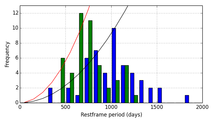
Figure 20: The frequency of supermassive black hole binaries as a function of restframe period. This shows the distribution for objects with $\log(M_{BH}/M_{\odot})<9$ (blue) and $\log(M_{BH}/M_{\odot})>9$ (green). Theoretical curves are also shown for a $n_{var}\propto t_{orb}^{8/3}$ relationship for the two mass distributions: $\log(M_{BH}/M_{\odot})<9$ (black) and $\log(M_{BH}/M_{\odot})>9$ (red).

7 Gravitational wave detection

Given that some of the candidates appear to be in the gravitational-wave driven phase of merging, it is worth determining whether any of them might be resolvable as individual sources for current or upcoming nanohertz GW detectors (pulsar timing arrays (PTA)) rather than just be contributors to the stochastic GW background. For each candidate, we have determined the maximum signal that could be detected (see Table 2). The GW frequency of a binary with a circular orbit is $f_{GW}=2/t_{per}$, where $t_{per}$ is the orbital period. The intrinsic GW strain amplitude is:

$$h_{s}=\left(\frac{128}{15}\right)^{1/2}\frac{(GM_{c})^{5/3}}{c^{4}d_{L}}(\pi f)^{2/3}$$

where $M_{c}=(M_{1}M_{2})^{3/5}(M_{1}+M_{2})^{-1/5}$ is the chirp mass and $d_{L}$ is the comoving distance to the source. The maximum induced timing residual amplitude is then $h_{s}/(2\pi f_{GW})$.

We have also calculated the inspiral time for each candidate (see Table 2) to check that there is no significant frequency evolution over the lifetime of a detection experiment, i.e., $t_{expt}<<t_{insp}$, where $t_{insp}=5(1+q)^{2}a^{4}/2qR_{S}^{3}$ and $R_{S}=2GM/c^{2}$. The median inspiral time is $\sim$8,000 years, although there are four candidates predicted to merge within the next century and , with decadal baselines, we should be able to detect period changes in these objects.

Using PTA noise estimates for Nanograv and the Parkes PTA (Arzoumanian et al. 2014 ; Zhu et al. 2014 ), we calculate that none of the candidates will be resolvable as sources by the current generation of experiments (see Fig. 21). However, some of the sources will be viable by the next generation of detectors, e.g., SKA.

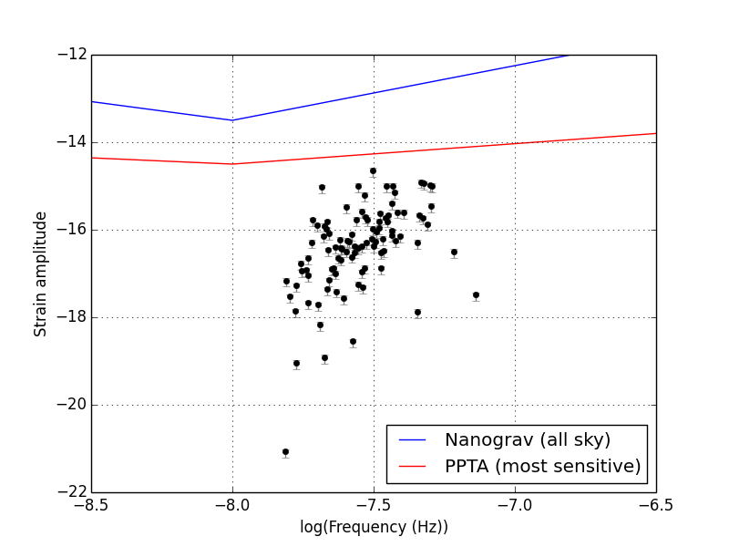
Figure 21: The expected GW strain amplitude for the candidate sources. The error bars indicate the range of strain amplitudes for $q=0.05$ to $q=1$. The blue line indicates the all-sky averaged noise limit for the Nanograv experiment and the red line that of the most sensitive detection limit for the Parkes PTA.

8 Conclusions

We have detected strong periodicity in the optical photometry of 111 quasars which we ascribe to the presence of a close SMBH binary in these systems. The Keplerian nature of the signal suggests that it is kinematic in origin and may be produced by a precessing jet, warped accretion disk or periodic accretion driven by the SMBH binary. We note our detection methodology may not be particularly sensitive to other types of periodic behavior exhibited by SMBH binary candidates, such as OJ 287. This would then suggest that our sample of objects represents a small fraction of a much larger close binary SMBH population which is yet to be detected. We are therefore planning further studies of the (quasi-)periodic quasar population with less stringent constraints than those applied in this analysis. This will also address our incomplete coverage of the gas-driven merger regime.

Further observations of our sample can test the different interpretations, as well as the primary SMBH binary attribution. Shen & Loeb (2010) suggest that reverberation mapping is a particularly useful diagnostic since the behaviour of emission line response to continuum variations is expected to be different for alternate explanations. We plan to see whether stacked reverberation employing time series and pairs of multiepoch spectra (Fine et al., 2013) is sufficient. Obviously continued monitoring by CRTS and other synoptic surveys will track future cycles of periodicity and historical photometric data from photographic plate collections, such as DASCH, may provide more data for previous cycles. For example, DASCH data for PG 1302-102 is consistent with the reported period (J. Grindlay, private communication). With such decadal baselines, any change in the period of the system expected from general relativity may be detectable.

Future spectroscopic observations can also test whether there is any spectral variation in the sample consistent with binary orbital timescales, although this is not necessarily present in such close systems. The theoretical expectation for pairs at the close separations that we are probing is that they should not show any such effect – the size of any broad line region (BLR) dwarfs the orbital dimensions of the binary and at separations closer than 0.03 pc in some scenarios, the BLR is truncated or destroyed (Ju et al., 2013). However, D’Orazio et al. (2015) suggest that there may be broadened emission due to recombination in orbiting circumbinary gas which would show as periodic variation in the FWHM of associated lines and smaller shifts in their centroids. Continued spectral monitoring, particularly coincident with an extremum in the photometric light curve, will help to confirm the origin of any spectral variability detected. With a binary, the variation should follow a regular evolution whereas a bright spot (non-axisymmetric perturbation in the BLR emissivity) in the BLR, say, should just be a transient feature. One caveat with any detection of spectral variability is that asymmetric reverberation can act as a major source of confusion noise in multiepoch spectroscopic data (Barth et al., 2015).

Multiwavelength observations, particularly of the radio quiet objects, will also provide more information about them. In particular, the specific predictions that D’Orazio et al. (2015) make regarding the Fe K$\alpha$ line, broad line widths and narrow line offsets for the accretion disc cavity model can be tested. Finally, we note that these objects are strong candidates for any gravitational wave experiment sensitive to nanohertz frequency waves such as those using pulsar timing arrays as well as any future space-borne gravitational wave detection mission.

References

- Alexander (2013) Alexander T., 2013, arXiv:1302.1508
- Andrae et al. (2013) Andrae R., Kim D. W., Bailer-Jones C. A. L., 2013, A&A, 554, A137, 11
- Artymowicz & Lubow (1996) Artymowicz P., Lubow S. H., 1996, ApJ, 467, L77
- (4) Arzoumanian Z., et al., 2014, ApJ, 794, 141
- Barth et al. (2015) Barth A. J., et al., 2015, ApJS, in press (arXiv:1503.01146)
- Barrows et al. (2011) Barrows R. S., Lacy C. H. S., Kennefick D., Kennefick J., Seigar M. S., 2011, NewA, 16, 122
- Bogdanović et al. (2008) Bogdanović T., Smith B. D., Sigurdsson S., Eracleous M., 2008, ApJS, 174, 455
- Bogdanović (2015) Bogdanović T., 2015, Astrophysics and Space Science Proceedings, 40, 103
- Boroson & Lauer (2009) Boroson T., Lauer T. R., 2009, Nature, 458, 53
- Caproni & Abraham (2004) Caproni A., Abraham Z., 2004, ApJ, 602, 625
- Caproni et al. (2006) Caproni A., Livio M., Abraham Z., Mosquera Cuesta H. J., 2006, ApJ, 653, 112
- Ciaramella et al. (2004) Ciaramella A., et al., 2004, å, 419, 485
- Colpi (2014) Colpi M., 2014, Space Sci. Rev., 183, 189
- Dawson et al. (2013) Dawson K. S., et al., 2013, AJ, 145, 10
- Decarli et al. (2010) Decarli R., Dotti M., Montuori C., Liimets T., Ederoclite A., 2010, ApJ, 720, L93
- (16) Decarli R., et al., 2013, MNRAS, 433, 1492
- De Paolis, Ingrosso & Nucita (2002) De Paolis F., Ingrosso G., Nucita A. A., 2002, å, 388, 470
- Dotti et al. (2009) Dotti M., Montuori C,m Decarli R., Volonteri M., Colpi M., Haardt F., 2009, MNRAS, 398, 73
- Dotti & Hogg (2011) Dotti M., Hogg D. W., 2011, ApJ, 738, 20bb
- (20) Drake A. J., et al., 2009, ApJ, 696, 870
- (21) Drake A. J., et al., 2013, ApJ, 763, 32
- (22) Djorgovski S.G., et al., 2012, in The First Year of MAXI: Monitoring Variable X-ray Sources. Mihara T. & Serino M., eds. Special Publ. IPCR-127, 263. Tokyo: RIKEN.
- D’Orazio et al. (2015) D’Orazio D. J. D., Haiman Z., Duffell P., Farris B. D., MacFadyen A. I., 2015, MNRAS, submitted (arXiv:1502.0311)
- Edelson & Krolik (1988) Edelson R, Krolik J., 1988, ApJ, 333, 646
- (25) Eracleous M., Boroson T. A., Halpern J. P., Liu J., 2012, ApJS, 201, 23
- Farris et al. (2014) Farris B. D., Duffell P., MacFadyen A. I., Haiman Z., 2014, ApJ, 783, 134
- Fan et al. (2002) Fan J. H., et al., 2002, å, 381, 1
- Fine et al. (2013) Fine S., et al., 2013, MNRAS, 434, 16
- Foster (1996) Foster G., 1996, AJ, 112, 1709
- Fragile et al. (2007) Fragile P. C., Blaes O. M., Anninos P., Salmonson J. D., 2007, ApJ, 668, 417
- Ghisellini et al. (2010) Ghisellini G., et al., 2010, MNRAS, 405, 387
- Gibson et al. (2009) Gibson, R. R., et al., 2009, ApJ, 692, 758
- Graham et al. (2013) Graham M. J., Drake A. J., Djorgovski S. G., Mahabal A. A., Donalek C., Duan V., Maker A., 2013, MNRAS, 434, 3423
- (34) Graham M. J., Djorgovski S. G., Drake A. J., Mahabal A. A., Chang M., Stern D., Donalek C., Glikman E., 2014, MNRAS, 439, 703
- Graham et al. (2015) Graham M. J., et al., 2015, Nature, 518, 74
- Gültekin & Miller (2012) Gültekin K., Miller J. M., 2012, ApJ, 761, 90
- Haehnelt & Kaufmann (2002) Haehnelt M., Kaufmann G., 2002, MNRAS, 336, 61