Attractive Hubbard Model: Homogeneous Ginzburg – Landau Expansion and Disorder

Abstract

We derive Ginzburg – Landau (GL) expansion in disordered attractive Hubbard model within the combined Nozieres – Schmitt-Rink and DMFT+$\Sigma$ approximation. Restricting ourselves to the case of homogeneous expansion, we analyze disorder dependence of GL expansion coefficients on disorder for the wide range of attractive potentials $U$, from weak BCS coupling region to the strong coupling limit, where superconductivity is described by Bose – Einstein condensation (BEC) of preformed Cooper pairs. We show, that for the case of semi – elliptic “bare” density of states of conduction band, disorder influence on GL coefficients $A$ and $B$ before quadratic and fourth – order terms of the order parameter, as well as on the specific heat discontinuity at superconducting transition, is of universal nature at any strength of attractive interaction and is related only to the general widening of the conduction band by disorder. In general, disorder growth increases the values of coefficients $A$ and $B$, leading either to the suppression of specific heat discontinuity (in the weak coupling limit), or to its significant growth (in the strong coupling region). However, this behavior actually confirms the validity of the generalized Anderson theorem, as disorder dependence of superconducting critical temperature $T_{c}$, is also controlled only by disorder widening of conduction band (density of states).

I Introduction

The problem of superconductivity in BCS — BEC crossover region (and up to the strong coupling limit) has a long history, starting with early works by Leggett and Nozieres and Schmitt-Rink [Leggett, ; NS, ]. Probably the simplest model to study this crossover is Hubbard model with attractive interaction. The most successive approach to the studies of Hubbard model (both repulsive and attractive) is the dynamical mean field theory (DMFT) [pruschke, ; georges96, ; Vollh10, ]. Attractive Hubbard model was already studied within DMFT in a number of papers [Keller01, ; Toschi04, ; Bauer09, ; Koga11, ; JETP14, ]. However, up to now there are only few works, where disorder effects were taken into account, either in normal or superconducting phases of this model. Qualitative analysis of disorder effects upon critical temperature $T_{c}$ in BCS — BEC crossover region was presented in Ref. [PosSad, ], which claimed the validity of Anderson theorem in this region for the case of $s$-wave pairing. Diagrammatic analysis of disorder effects on $T_{c}$ and the properties of the normal state in crossover region was recently presented in Ref. [PalStr, ].

We have developed the generalized DMFT+$\Sigma$ approach to Hubbard model [JTL05, ; PRB05, ; FNT06, ; UFN12, ], which is quite convenient for the account of different “external” interactions, e.g. such as disorder scattering [HubDis, ; HubDis2, ]. This approach is also well suited to the studies of two–particle properties, such as dynamic (optical) conductivity [HubDis, ; PRB07, ]. In a recent paper [JETP14, ] we used this approach to analyze the single–particle properties of the normal phase and optical conductivity in attractive Hubbard model. Further on the DMFT+$\Sigma$ approximation was combined with Nozieres – Schmitt-Rink approach to study the influence of disorder on superconducting critical temperature $T_{c}$ in BCS – BEC crossover and strong coupling region [JTL14, ; JETP15, ], demonstrating the validity of the generalized Anderson theorem. Disorder effects upon $T_{c}$ are essentially due only the general widening of the conduction band by random scattering. This was demonstrated exactly (for the whole range of attractive interactions) in the case of semi – elliptic density of states of conduction band (three-dimensional case) at any disorder level and becomes also valid in the case of flat band (two-dimensional case) in the limit of strong enough disorder.

Ginzburg – Landau (GL) expansion in the region of BCS – BEC crossover was derived in a number of previous papers [Micnas01, ; Zwerger92, ; Zwerger97, ], however no effects of disorder scattering on GL – expansion coefficients was considered. Here we derive the microscopic coefficients of (homogeneous) GL – expansion for the attractive Hubbard model and study disorder effects on these coefficients including the BCS – BEC and strong coupling regions, as well as upon the specific heat discontinuity at superconducting transition, demonstrating certain universality of disorder behavior of these characteristics..

II Disordered Hubbard model in DMFT+$\Sigma$ approach

We consider the disordered attractive Hubbard model with Hamiltonian:

$$H=-t\sum_{\langle ij\rangle\sigma}a_{i\sigma}^{\dagger}a_{j\sigma}+\sum_{i\sigma}\epsilon_{i}n_{i\sigma}-U\sum_{i}n_{i\uparrow}n_{i\downarrow},$$ (1)

where $t>0$ is transfer integral between the nearest neighbors and $U$ is onsite Hubbard attraction , $n_{i\sigma}=a_{i\sigma}^{\dagger}a_{i\sigma}^{{\phantom{\dagger}}}$ is electron number operator at site $i$, $a_{i\sigma}$ ($a_{i\sigma}^{\dagger}$) is annihilation (creation) operator of an electron with spin $\sigma$. Local energy levels $\epsilon_{i}$ are assumed to be independent random variables on different lattice sites. We assume the Gaussian distribution of $\epsilon_{i}$ at each site for the validity of the standard “impurity” scattering diagram technique [Diagr, ]:

$$\mathcal{P}(\epsilon_{i})=\frac{1}{\sqrt{2\pi}\Delta}\exp\left(-\frac{\epsilon_{i}^{2}}{2\Delta^{2}}\right)$$ (2)

Here $\Delta$ is the measure of disorder scattering.

The generalized DMFT+$\Sigma$ approach [JTL05, ; PRB05, ; FNT06, ; UFN12, ] supplies the standard DMFT [pruschke, ; georges96, ; Vollh10, ] with an additional “external” self-energy (in general case momentum dependent) due to any interaction outside the DMFT, which provides an effective method to calculate both single and two – particle properties [HubDis, ; PRB07, ]. The additive form of the total self-energy conserves the structure of self – consistent equations of DMFT [pruschke, ; georges96, ; Vollh10, ]. The “external” self-energy is recalculated at each step of the standard DMFT iteration scheme, using some approximations, corresponding to the form of an additional interaction, while the local Green’s function (central for DMFT) is also “dressed” by additional interaction.

For disordered Hubbard model we take the “external” self-energy entering DMFT+$\Sigma$ cycle in the simplest form of self – consistent Born approximation, neglecting the “crossing” diagrams due to disorder scattering:

$$\tilde{\Sigma}(\varepsilon)=\Delta^{2}\sum_{\bf p}G(\varepsilon,{\bf p}),$$ (3)

where $G(\varepsilon,{\bf p})$ is the complete single – particle Green’s function.

To solve the effective Anderson impurity model of DMFT here we used the effective algorithm of numerical renormalization group (NRG) [NRGrev, ].

In the following, we consider the model of the “bare” conduction band with semi – elliptic density of states (per unit cell and spin projection):

$$N_{0}(\varepsilon)=\frac{2}{\pi D^{2}}\sqrt{D^{2}-\varepsilon^{2}}$$ (4)

where $D$ determines the half – width of conduction band. This is a good approximation for the three – dimensional case.

In Ref. [JETP15, ] we have shown analytically, that in DMFT+$\Sigma$ approach, within these approximations, all the disorder influence upon single – particle properties is reduced to the simple effect of band widening by disorder scattering, so that $D\to D_{eff}$, where $D_{eff}$ is the effective band half – width in the presence of disorder (in the absence of correlations, i.e. for $U=0$):

$$D_{eff}=D\sqrt{1+4\frac{\Delta^{2}}{D^{2}}}.$$ (5)

and conduction band density of states (in the absence of $U$) “dressed” by disorder is given by:

$$\tilde{N}_{0}(\varepsilon)=\frac{2}{\pi D_{eff}^{2}}\sqrt{D_{eff}^{2}-\varepsilon^{2}}$$ (6)

conserving its semi – elliptic form.

For other models of the “bare” conduction band density of states, besides band widening, disorder scattering changes the form of the density of states, so that the complete universality of disorder influence of single – particle properties, strictly speaking, is absent. However, in the limit of strong enough disorder the “bare” band density effectively becomes elliptic for any reasonable model, so that universality is restored [JETP15, ].

All calculation below were performed for the quarter – filled band (n=0.5 per lattice site).

III Ginzburg – Landau expansion

The critical temperature of superconducting transition $T_{c}$ in attractive Hubbard model was analyzed using direct DMFT calculations a number of papers [Keller01, ; Toschi04, ; Koga11, ]. In Ref. [JETP14, ] we have determined $T_{c}$ from instability condition of the normal phase (instability of DMFT iteration procedure). The results obtained in this way were in good agreement with the results of Refs. [Keller01, ; Toschi04, ; Koga11, ]. Additionally, in Ref. [JETP14, ] we calculated $T_{c}$ using the approximate Nozieres – Schmitt–Rink approach in combination with DMFT (used to calculate the chemical potential of the system), demonstrating that being much less time consuming, it provides semi – quantitative description $T_{c}$ behavior in BCS – BEC crossover region, in good agreement with direct DMFT calculations. In Refs. [JTL14, ; JETP15, ] the combined Nozieres – Schmitt-Rink approach was used to study the detailed dependence of $T_{c}$ on disorder. Below we shall use this combined approach to derive GL – expansion including the disorder dependence of GL – expansion coefficients.

We shall write GL – expansion for the difference of free energies of superconducting and normal phases in the standard form:

$$F_{s}-F_{n}=A|\Delta_{\bf q}|^{2}+q^{2}C|\Delta_{\bf q}|^{2}+\frac{B}{2}|\Delta_{\bf q}|^{4},$$ (7)

where $\Delta_{\bf q}$ is the spatial Fourier component of the amplitude of superconducting order parameter. Microscopically, this expansion is determined by diagrams of the loop – expansion for the free energy of an electron in the “external field” of (static) superconducting order parameter fluctuations with small wave vector ${\bf q}$ , shown in Fig.1 (where fluctuations are represented by dashed lines) [Diagr, ]. Below we limit ourselves to the case of homogeneous expansion with ${\bf q}=0$ and calculations of its coefficients $A$ and $B$, leaving the (much more complicated) analysis of the general inhomogeneous case of finite ${\bf q}$ and calculations of coefficient $C$ in (7) for the future work.

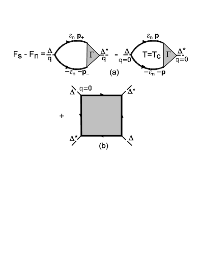
Figure 1: Diagrammatic representation of Ginzburg – Landau expansion.

Within Nozieres – Schmitt-Rink approach [NS, ] we use the weak coupling approximation to calculate loop – diagrams with two and four Cooper vertices shown in Fig. 1, dropping all corrections due to Hubbard $U$, while including “dressing” by disorder scattering. However, the chemical potential, which essentially depends on the coupling strength $U$ and determines the condition of BEC in the strong coupling region, is calculated via the full DMFT+$\Sigma$ procedure.

Coefficient $A$ before the square of the order parameter in GL – expansion is given by diagrams of Fig. 1(a) with $q=0$ [Diagr, ]:

$$A(T)=\chi_{0}(q=0,T)-\chi_{0}(q=0,T_{c}),$$ (8)

where

$$\chi_{0}(q=0,T)=-T\sum_{n}\sum_{\bf pp^{\prime}}\Phi_{\bf pp^{\prime}}(\varepsilon_{n})$$ (9)

is the two – particle loop in Cooper channel “dressed” only by disorder scattering, while $\Phi_{\bf pp^{\prime}}(\varepsilon_{n})$ is disorder averaged two – particle Green’s function in Cooper channel ($\varepsilon_{n}=\pi T(2n+1)$ is corresponding Matsubara frequency). Subtraction of the second diagram in Fig. 1(a), i.e. that of $\chi_{0}(q=0,T_{c})$ in (8), guarantees the validity of $A(T=T_{c})=0$, which is necessarily so in any kind of Landau expansion [Diagr, ].

To obtain $\sum_{\bf pp^{\prime}}\Phi_{\bf pp^{\prime}}(\varepsilon_{n})$ we use an exact Ward identity, derived in Ref. [PRB07, ]:

$$G(\varepsilon_{n},{\bf p})-G(-\varepsilon_{n},-{\bf p})=$$

$$=-\sum_{\bf p^{\prime}}\Phi_{\bf pp^{\prime}}(\varepsilon_{n})(G_{0}^{-1}(\varepsilon_{n},{\bf p^{\prime}})-G_{0}^{-1}(-\varepsilon_{n},-{\bf p^{\prime}})),$$ (10)

Here $G(\varepsilon_{n},{\bf p})$ is disorder averaged (but not “dressed” by Hubbard interaction!) single – particle Green’s function. Using the symmetry $\varepsilon({\bf p})=\varepsilon(-{\bf p})$ and $G(\varepsilon_{n},-{\bf p})=G(\varepsilon_{n},{\bf p})$, we obtain from the Ward identity (10):

$$\sum_{\bf pp^{\prime}}\Phi_{\bf pp^{\prime}}(\varepsilon_{n})=-\frac{\sum_{\bf p}G(\varepsilon_{n},{\bf p})-\sum_{\bf p}G(-\varepsilon_{n},{\bf p})}{2i\varepsilon_{n}},$$ (11)

so that for Cooper susceptibility (9) we get:

$$\chi_{0}(q=0,T)=$$

$$=T\sum_{n}\frac{\sum_{\bf p}G(\varepsilon_{n},{\bf p})-\sum_{\bf p}G(-\varepsilon_{n},{\bf p})}{2i\varepsilon_{n}}=$$

$$=T\sum_{n}\frac{\sum_{\bf p}G(\varepsilon_{n},{\bf p})}{i\varepsilon_{n}}.$$ (12)

Performing now the standard summation over Matsubara frequencies [Diagr, ], we obtain:

$$\chi_{0}(q=0,T)=$$

$$=\frac{1}{4\pi i}\int_{-\infty}^{\infty}d\varepsilon\frac{\sum_{\bf p}G^{R}(\varepsilon,{\bf p})-\sum_{\bf p}G^{A}(\varepsilon,{\bf p})}{\varepsilon}th\frac{\varepsilon}{2T}=$$

$$=-\int_{-\infty}^{\infty}d\varepsilon\frac{\tilde{N}(\varepsilon)}{2\varepsilon}th\frac{\varepsilon}{2T},$$ (13)

where $\tilde{N}(\varepsilon)$ is the “bare” ($U=0$) density of states, “dressed” by disorder scattering, which in the case of semi – elliptic band takes the form (6). In Eq. (13) the origin of $\varepsilon$ is at the chemical potential. Replacing $\varepsilon\to\varepsilon-\mu$ to move the origin of energy to the center of conduction band, we finally write:

$$\chi_{0}(q=0,T)=-\int_{-\infty}^{\infty}d\varepsilon\frac{\tilde{N}(\varepsilon)}{2(\varepsilon-\mu)}th\frac{\varepsilon-\mu}{2T},$$ (14)

Cooper instability of the normal phase, determining superconducting transition temperature $T_{c}$, is written as:

$$1=-U\chi_{0}(q=0,T_{c})$$ (15)

Then, to determine the critical temperature we obtain the following equation:

$$1=\frac{U}{2}\int_{-\infty}^{\infty}d\varepsilon\tilde{N}_{0}(\varepsilon)\frac{th\frac{\varepsilon-\mu}{2T_{c}}}{\varepsilon-\mu},$$ (16)

Using (15) to determine $\chi_{0}(q=0,T_{c})$ and (14) for $\chi_{0}(q=0,T)$, we obtain the coefficient $A$ (8):

$$A(T)=\frac{1}{U}-\int_{-\infty}^{\infty}d\varepsilon\tilde{N}_{0}(\varepsilon)\frac{th\frac{\varepsilon-\mu}{2T}}{2(\varepsilon-\mu)}.$$ (17)

The chemical potential for different values of $U$ and $\Delta$ is to be determined here from direct DMFT+$\Sigma$ calculations, i.e. from the standard equation for the total number of electrons (band filling), defined by Green’s function obtained in DMFT+$\Sigma$ approximation. This allows us to find both $T_{c}$ and GL – expansion coefficients in the wide range of parameters of the model, including the BCS – BEC crossover region and the limit of strong coupling, for different disorder levels. Actually, this is the essence of Nozieres – Schmitt-Rink approximation — in the weak coupling region transition temperature is controlled by the equation for Cooper instability, while in the strong coupling limit it is defined as the temperature of Bose condensation, which is controlled by the equation for chemical potential. The joint solution of Eqs. (16) and (17) with DMFT+$\Sigma$ equation for chemical potential provides the correct interpolation for $T_{c}$ and GL – coefficient $A$ from weak coupling region via the BCS – BEC crossover towards the strong coupling.

For $T\to T_{c}$ the coefficient $A(T)$ is written as:

$$A(T)\equiv a(T-T_{c}).$$ (18)

where in case of temperature independent chemical potential

$$a=\frac{1}{4T_{c}^{2}}\int_{-\infty}^{\infty}d\varepsilon\tilde{N}_{0}(\varepsilon)\frac{1}{ch^{2}\frac{\varepsilon-\mu}{2T_{c}}}.$$ (19)

In BCS approximation with conduction band of infinite width with constant density of states $\tilde{N}_{0}(0)$ we obtain from (19) the standard result $a=\frac{\tilde{N}_{0}(0)}{T_{c}}$ [Diagr, ]. However, in BCS – BEC crossover region temperature dependence of $\mu$ is essential and we have to use the general expression (17) in conjunction with equation for $\mu$ to calculate $a$. At the same time, from Eq. (17) it is clear that disorder scattering influences $a$ only through the changes of the density of states $\tilde{N}_{0}(\varepsilon)$ and chemical potential $\mu$, which is the typical single – particle property. Thus, in the case of semi – elliptic “bare” conduction band the dependence of $a$ on disorder is due only to the band widening by disorder replacing $D\to D_{eff}$. Thus, in the presence of disorder we expect the universal dependence of $a(2D_{eff})^{2}$ on $U/2D_{eff}$ (all energies are to be normalized by the effective bandwidth $2D_{eff}$), which will be confirmed by the results of direct numerical computations in the next Section (cf. Fig. 4(a)).

Coefficient $B$ is determined by “square” diagram with four Cooper vertices with ${\bf q}=0$, “dressed” in arbitrary way by disorder scattering, which is shown in Fig. 1(b) [Diagr, ]:

$$B=\frac{1}{2}T\sum_{n}\sum_{{\bf p}_{1}{\bf p}_{2}{\bf p}_{3}{\bf p}_{4}}<G(i\varepsilon_{n};{\bf p}_{1},{\bf p}_{2})G(-i\varepsilon_{n};-{\bf p}_{2},-{\bf p}_{3})$$

$$G(i\varepsilon_{n};{\bf p}_{3},{\bf p}_{4})G(-i\varepsilon_{n};-{\bf p}_{4},-{\bf p}_{1})>,$$

(20)

where $<\cdots>$ denotes averaging over disorder, while $G(i\varepsilon_{n};{\bf p}_{1},{\bf p}_{2})$ (and other similar expressions) represent exact single – particle Green’s functions for the fixed configuration of the random potential. Performing standard summation over Matsubara frequencies, we obtain:

$$B=\frac{1}{2}\int_{-\infty}^{\infty}\frac{d\varepsilon}{2\pi i}th\frac{\varepsilon}{2T}\sum_{\bf p_{1}p_{2}p_{3}p_{4}}<G^{R}(\varepsilon;{\bf p_{1}},{\bf p_{2}})$$

$$G^{A}(-\varepsilon;-{\bf p_{2}},-{\bf p_{3}})G^{R}(\varepsilon;{\bf p_{3}},{\bf p_{4}})G^{A}(-\varepsilon;-{\bf p_{4}},-{\bf p_{1}})>.$$

(21)

Due to zero value of momentum ${\bf q}=0$ in Cooper vertices and the static nature of disorder scattering, we can now use certain generalization of the Ward identity (10) to get (at $T=T_{c}$):

$$B=\int_{-\infty}^{\infty}\frac{d\varepsilon}{4\varepsilon^{3}}\left(th\frac{\varepsilon}{2T_{c}}-\frac{\varepsilon/2T_{c}}{ch^{2}\frac{\varepsilon}{2T_{c}}}\right)\tilde{N}_{0}(\varepsilon)$$ (22)

Detailed derivation is presented in Appendix A. In BCS approximation, using the conduction band of infinite width with constant density of states $\tilde{N}_{0}(0)$, we immediately obtain from Eq. (22) the standard result: $B=\frac{7\zeta(3)}{8\pi^{2}T_{c}^{2}}\tilde{N}_{0}(0)$ [Diagr, ].

Again, replacing here $\varepsilon\to\varepsilon-\mu$, to move the origin of energy to the middle of the conduction band, we can write:

$$B=\int_{-\infty}^{\infty}\frac{d\varepsilon}{4(\varepsilon-\mu)^{3}}\left(th\frac{\varepsilon-\mu}{2T_{c}}-\frac{(\varepsilon-\mu)/2T_{c}}{ch^{2}\frac{\varepsilon-\mu}{2T_{c}}}\right)\tilde{N}_{0}(\varepsilon)$$ (23)

It is seen, that disorder dependence of the coefficient $B$ (similarly to $A$) is also determined only by disorder widened density of states $\tilde{N}_{0}(\varepsilon)$ and chemical potential, so that in the case of semi – elliptic “bare” conduction band it is reduced to simple replacement $D\to D_{eff}$, leading to universal dependence of $B(2D_{eff})^{3}$ on $U/2D_{eff}$, which is confirmed by the results of direct numerical computations presented in the next Section and shown in Fig.4b.

It should be stressed, that Eqs. (17) and (23) for GL – coefficients $A$ and $B$ were obtained with the use of exact Ward identities, and are thus valid also in the limit of strong disorder (beyond Anderson localization).

Universal dependence on disorder, related to conduction band widening by disorder scattering, is also valid for specific heat discontinuity at $T_{c}$, as it is completely determined by coefficients $a$ and $B$:

$$C_{s}(T_{c})-C_{n}(T_{c})=T_{c}\frac{a^{2}}{B}$$ (24)

Appropriate numerical results are also given in the next Section (cf. Fig. 5(b)).

Coefficient $C$ before the gradient term of GL – expansion is determined essentially by two – particle characteristics (due in particular to non – trivial $q$ – dependence of the vertex, which is obviously changed by disorder scattering). In particular, the behavior of $C$ is significantly changed at Anderson transition [SCLoc, ], so that no universality of disorder dependence is expected in this case.

IV Main results

Let us now discuss the main results of our numerical calculations, directly demonstrating the universal dependencies of GL – coefficients $A$ and $B$ and specific heat discontinuity at $T_{c}$ on disorder.

In Fig. 2 we show the universal dependence of critical temperature $T_{c}$ on Hubbard attraction $U$ for different levels of disorder, which was obtained and discussed in detail in Refs. [JTL14, ; JETP15, ]. Typical maximum of $T_{c}$ at $U/2D_{eff}\sim 1$ is characteristic of BCS – BEC crossover region.

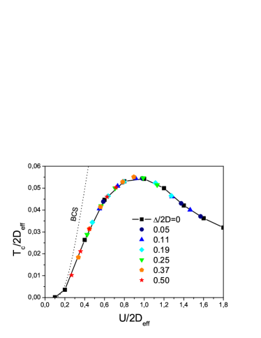
Figure 2: Universal dependence of superconducting critical temperature on disorder for different values of Hubbard attraction.

In Fig. 3 we present disorder dependencies of GL – coefficients $a$ (Fig. 3(a)) and $B$ (Fig. 3(b)) for different values of Hubbard attraction. We can see that $a$ in general increases with the growth of disorder. Only in the limit of strong enough coupling $U/2D>1.4$ (curves 4 and 5) in the region of weak disorder we observe weak suppression of $a$ by disorder scattering. Coefficient $B$ pretty fast grows with disorder in the region of weak coupling (curve 1 in Fig. 3(b)), while in the region of strong coupling this growth becomes more moderate (curves 4,5 in Fig. 3(b), so that in this region the dependence of $B$ on disorder becomes almost independent of the value of $U$ (curves 4 and 5 practically coincide).

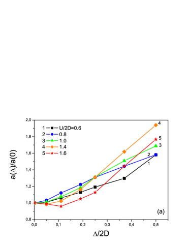
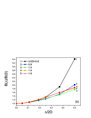
Figure 3: Disorder dependence of GL – coefficients $a$ (a) and $B$ (b), normalized by their values in the absence of disorder, for different values of Hubbard attraction.

However, this rather complicated dependence of coefficients $a$ and $B$ on disorder is determined solely by the growth of effective conduction bandwidth with disordering given by Eq. (5). In Fig. 4 we show the universal dependencies of GL – coefficients $a$ (a) and $B$ (b), normalized by appropriate powers of effective bandwidth, on the strength of Hubbard attraction. In the absence of disorder (dashed line with squares) coefficients $a$ and $B$ drop fast with the growth of $U$. Other symbols in Fig. 4 show the results of our calculations for different levels of disorder. It is clearly seen, that all the data ideally fit the universal curve, obtained in the absence of disorder.

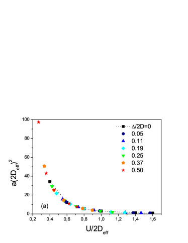
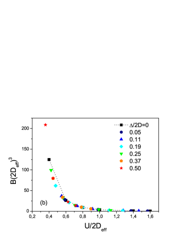
Figure 4: Universal dependence of GL – coefficients $a$ (a) and $B$ (b) on Hubbard attraction for different values of disorder.

Coefficients $a$ and $B$ determine specific heat discontinuity at the critical temperature (24). As these coefficients and $T_{c}$ [JTL14, ; JETP15, ] depend on disorder in universal way due only to the growth of the effective bandwidth (5), the same type of universal dependence is also valid for specific heat discontinuity. In Fig. 5(a) we show the dependence of specific heat discontinuity $dC\equiv C_{s}-C_{n}$ on disorder for different values of Hubbard attraction $U$. It is seen, that in the region of weak coupling (curve 1) specific heat discontinuity is suppressed by disordering, for intermediate couplings (curves 2,3) weak disorder leads to the growth of specific heat discontinuity, while the further growth of disorder suppresses this discontinuity. In the region of strong coupling (curves 4,5) the growth of disorder leads to significant growth of specific heat discontinuity, which is mainly related to the similar growth of $T_{c}$ (cf. [JTL14, ; JETP15, ]). However, this complicated dependence of specific heat discontinuity on disorder is again completely determined by the growth of the effective bandwidth (5). In Fig.5(b) we show the universal dependence of specific heat discontinuity on $U$, normalized by the bandwidth $2D_{eff}$. Black squares represent data in the case of absence of disorder. Other symbols in Fig. 5(b) show the data for different disorder levels. It is seen again, that all the data precisely fit the universal dependence of specific heat discontinuity obtained in the absence of disorder. Specific heat discontinuity grows with the growth of $U$ in the region of weak coupling $U/2D_{eff}\ll 1$ and drops with the growth of $U$ in the limit of strong coupling $U/2D_{eff}\gg 1$. The maximum of specific heat discontinuity is observed at $U/2D_{eff}\approx 0.55$. Actually, this dependence of specific heat discontinuity qualitatively resembles the similar dependence of critical temperature, though the its maximum is reached at smaller values of Hubbard attraction.

V Conclusion

Using the combination of Nozieres – Schmitt-Rink approximation with the generalized DMFT+$\Sigma$ approach we have studied disorder influence upon coefficients $A$ and $B$ determining the homogeneous Ginzburg — Landau expansion and specific heat discontinuity at superconducting transition in attractive Hubbard model.

We have demonstrated analytically, that in the case of the “bare” conduction band with semi – elliptic density of states disorder influence on GL – coefficients $A$ and $B$ and specific heat discontinuity is universal and is controlled only by the general conduction band (density of states) widening by disorder scattering and illustrated this conclusion with explicit numerical calculations, performed for the wide range of attractive potentials $U$, from weak coupling region where $U/2D_{eff}\ll 1$ and superconducting instability is described by the usual BCS approach, up to the strong coupling region where $U/2D_{eff}\gg 1$ and superconducting transition is determined by Bose – Einstein condensation of preformed Cooper pairs.

These results essentially prove the validity of the generalized Anderson theorem in BCS – BEC crossover region and in the limit of strong coupling not only for superconducting $T_{c}$ [JTL14, ; JETP15, ], but also for homogeneous Ginzburg – Landau expansion, determining appropriate thermodynamic effects, like specific heat discontinuity at transition point.

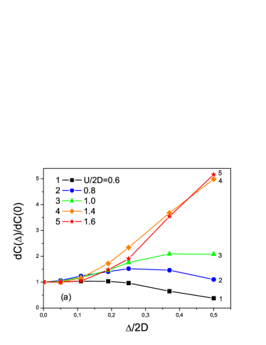
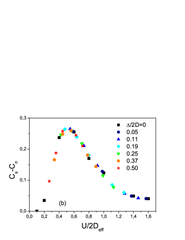
Figure 5: Dependence of specific heat discontinuity at critical temperature $dC\equiv C_{s}-C_{n}$ on disorder for different values of Hubbard attraction $U$ (a) and universal dependence of this discontinuity on $U$ for different values of disorder (b).

This work is supported by RSF grant 14-12-00502.

Appendix A Coefficient $B$ in the presence of disorder

Coefficient $B$ is determined by “square” diagram with four Cooper vertices with ${\bf q}=0$, “dressed” by disorder scattering, shown in Fig. 1(b). Corresponding analytic expression was given above in Eq. (20). After the standard summation over Matsubara frequencies $B$ is written as in (21), i.e. is determined by the following combination of four Green’s functions with real frequencies:

$$\sum_{\bf p_{1}p_{2}p_{3}p_{4}}<G^{R}(\varepsilon;{\bf p_{1}},{\bf p_{2}})G^{A}(-\varepsilon;-{\bf p_{2}},-{\bf p_{3}})$$

$$G^{R}(\varepsilon;{\bf p_{3}},{\bf p_{4}})G^{A}(-\varepsilon;-{\bf p_{4}},-{\bf p_{1}})>.$$ (25)

where $<\cdots>$ denotes averaging over disorder and $G^{R(A)}(\varepsilon;{\bf p}_{1},{\bf p}_{2})$ are the exact retarded (advanced) single – particle Green’s functions for the fixed configuration of disorder.

Typical diagram for the fourth order of disorder scattering (dashed lines) is shown in Fig. 6(a). Arbitrary diagrams for such four – particle Green’s function can be obtained from diagrams for single – particle Green’s function of the same order of disorder scattering by arbitrary inserting three Cooper vertices into “bare” electron Green’s functions, as shown in Fig. 6(a). Taking into account the static nature of disorder scattering and zero value of transferred momentum ${\bf q}=0$ in Cooper vertices, we can evaluate (25) using certain generalization of exact Ward identity (10), derived in Ref. [PRB07, ].

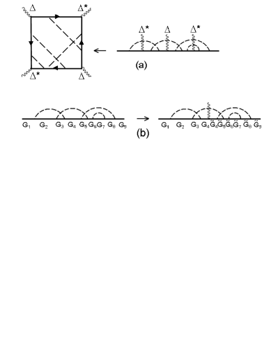
Figure 6: Diagrams for coefficient $B$ and derivation of the generalized Ward identity.

Let us take the diagram for single – particle Green’ function, shown in the left part of Fig. 6(b), and consider certain configuration of momenta transferred by dashed lines. Here we have nine “bare” electron Green’s functions with momenta ${\bf p}_{1}\cdots{\bf p}_{9}$. In the following we use short notations:

$$G_{i}=G_{0}^{R}(\varepsilon;{\bf p_{i}})\qquad\tilde{G}_{i}=G_{0}^{A}(-\varepsilon;-{\bf p_{i}}),$$ (26)

where $G_{0}^{R(A)}(\varepsilon;{\bf p})=\frac{1}{\varepsilon-\varepsilon({\bf p})\pm i\delta}$ is the “bare” Green’s function. Insertion of Cooper vertex leads to the sign change of momenta and frequencies (i.e. to the replacement $G_{i}\leftrightarrow\tilde{G}_{i}$) in all Green’s functions standing to the right from the vertex. Let us assume, that the central of three Cooper vertices was inserted in the fourth Green’s function, as shown in the right part of Fig. 6(b). Arbitrary insertion of the first Cooper vertex into one of the first four of Green’s functions leads to the following result:

$$G_{1}G_{2}G_{3}G_{4}\to G_{1}\tilde{G}_{1}\tilde{G}_{2}\tilde{G}_{3}\tilde{G}_{4}+G_{1}G_{2}\tilde{G}_{2}\tilde{G}_{3}\tilde{G}_{4}+$$

$$G_{1}G_{2}G_{3}\tilde{G}_{3}\tilde{G}_{4}+G_{1}G_{2}G_{3}G_{4}\tilde{G}_{4},$$ (27)

so that taking into account $G_{i}^{-1}-\tilde{G}_{i}^{-1}=2\varepsilon$, we get:

$$G_{1}\tilde{G}_{1}\tilde{G}_{2}\tilde{G}_{3}\tilde{G}_{4}\frac{G_{1}^{-1}-\tilde{G}_{1}^{-1}}{2\varepsilon}+\cdots$$

$$+G_{1}G_{2}G_{3}G_{4}\tilde{G}_{4}\frac{G_{4}^{-1}-\tilde{G}_{4}^{-1}}{2\varepsilon}=$$

$$=\frac{\tilde{G}_{1}\tilde{G}_{2}\tilde{G}_{3}\tilde{G}_{4}-G_{1}G_{2}G_{3}G_{4}}{2\varepsilon}$$ (28)

Then $\tilde{G}_{4}\tilde{G}_{5}\tilde{G}_{6}\tilde{G}_{7}\tilde{G}_{8}\tilde{G}_{9}\to G_{4}G_{5}G_{6}G_{7}G_{8}G_{9}$ and after all insertions of the last (third) Cooper vertex in one of the six Green’s functions $G_{4}\cdots G_{9}$, we again obtain: $\frac{\tilde{G}_{4}\tilde{G}_{5}\tilde{G}_{6}\tilde{G}_{7}\tilde{G}_{8}\tilde{G}_{9}-G_{4}G_{5}G_{6}G_{7}G_{8}G_{9}}{2\varepsilon}$.

Thus we get:

$$<G^{R}(\varepsilon)G^{A}(-\varepsilon)G^{R}(\varepsilon)G^{A}(-\varepsilon)>=$$

$$=<\frac{G^{A}(-\varepsilon)-G^{R}(\varepsilon)}{2\varepsilon}\frac{G^{A}(-\varepsilon)-G^{R}(\varepsilon)}{2\varepsilon}>=$$

$$=\frac{1}{4\varepsilon^{2}}(<G^{A}(-\varepsilon)G^{A}(-\varepsilon)>+<G^{R}(\varepsilon)G^{R}(\varepsilon)>-$$

$$-2<G^{R}(\varepsilon)G^{A}(-\varepsilon)>)=$$

$$=\frac{1}{4\varepsilon^{2}}\left\{\frac{d}{d\varepsilon}(<G^{A}(-\varepsilon)>-<G^{R}(\varepsilon)>)-\right.$$

$$\left.-\frac{<G^{A}(-\varepsilon)>-<G^{R}(\varepsilon)>}{\varepsilon}\right\},$$ (29)

where we can evaluate two – particle Green’s functions with $q=0$ again using the analogue of the Ward identity (10) for real frequencies. Using (29) in (21) and making in terms with $<G^{A}(-\varepsilon)>$ under the integral over $\varepsilon$ the replacement $\varepsilon\to-\varepsilon$, we obtain the following expression for coefficient $B$:

$$B=\int_{-\infty}^{\infty}\frac{d\varepsilon}{2\pi i}\frac{th\frac{\varepsilon}{2T}}{4\varepsilon^{2}}\times$$

$$\times\left(\frac{d}{d\varepsilon}-\frac{1}{\varepsilon}\right)(\sum_{\bf p}G^{A}(\varepsilon,{\bf p})-\sum_{\bf p}G^{R}(\varepsilon,{\bf p}))=$$

$$=\int_{-\infty}^{\infty}d\varepsilon\frac{th\frac{\varepsilon}{2T}}{4\varepsilon^{2}}\left(\frac{d}{d\varepsilon}-\frac{1}{\varepsilon}\right)\tilde{N}_{0}(\varepsilon)=$$

$$=\int_{-\infty}^{\infty}\frac{d\varepsilon}{4\varepsilon^{3}}\left(th\frac{\varepsilon}{2T}-\frac{\varepsilon/2T}{ch^{2}\frac{\varepsilon}{2T}}\right)\tilde{N}_{0}(\varepsilon)$$ (30)

which was used in the main part of the paper.

References

- (1) A. J. Leggett, in Modern Trends in the Theory of Condensed Matter, edited by A. Pekalski and J. Przystawa (Springer, Berlin 1980).
- (2) P. Nozieres and S. Schmitt-Rink, J. Low Temp. Phys. 59, 195 (1985)
- (3) Th. Pruschke, M. Jarrell, and J. K. Freericks, Adv. in Phys. 44, 187 (1995).
- (4) A. Georges, G. Kotliar, W. Krauth, and M. J. Rozenberg, Rev. Mod. Phys. 68, 13 (1996).
- (5) D. Vollhardt in “Lectures on the Physics of Strongly Correlated Systems XIV”, eds. A. Avella and F. Mancini, AIP Conference Proceedings vol. 1297 (American Institute of Physics, Melville, New York, 2010), p. 339; ArXiV: 1004.5069
- (6) M. Keller, W. Metzner, and U. Schollwock. Phys. Rev. Lett. 86, 4612-4615 (2001); ArXiv: cond-mat/0101047
- (7) A. Toschi, P. Barone, M. Capone, and C. Castellani. New Journal of Physics 7, 7 (2005); ArXiv: cond-mat/0411637v1
- (8) J. Bauer, A.C. Hewson, and N. Dupis. Phys. Rev. B 79, 214518 (2009); ArXiv: 0901.1760v2
- (9) A. Koga and P. Werner. Phys. Rev. A 84, 023638 (2011); ArXiv: 1106.4559v1
- (10) N.A. Kuleeva, E.Z. Kuchinskii, M.V. Sadovskii. Zh. Eksp. Teor. Fiz. 146, No. 2, 304 (2014); [JETP 119, No. 2, 264-271 (2014)]; ArXiv: 1401.2295
- (11) A.I. Posazhennikova and M.V. Sadovskii. Pisma Zh. Eksp. Teor. Fiz. 65, 258 (1997) [JETP Letters 65, 270 (1997)]
- (12) F. Palestini, G.C. Strinati. ArXiv:1311.2761
- (13) E.Z.Kuchinskii, I.A.Nekrasov, M.V.Sadovskii. Pisma Zh. Eksp. Teor. Fiz. 82, No. 4, 217 (2005) [JETP Lett. 82, 198 (2005)]; ArXiv: cond-mat/0506215.
- (14) M.V. Sadovskii, I.A. Nekrasov, E.Z. Kuchinskii, Th. Pruschke,V.I. Anisimov. Phys. Rev. B 72, No 15, 155105 (2005); ArXiV: cond-mat/0508585
- (15) E.Z. Kuchinskii, I.A. Nekrasov, M.V. Sadovskii. Fizika Nizkih Temperatur 32, No. 4/5, 528-537 (2006); [Low Temp. Phys. 32, 398 (2006)]; ArXiv: cond-mat/0510376
- (16) E.Z. Kuchinskii, I.A. Nekrasov, M.V. Sadovskii. Usp. Fiz. Nauk 182, No. 4, 345-378 (2012); [Physics Uspekhi 55, No. 4, 325-355 (2012)]; ArXiv:1109.2305
- (17) E.Z. Kuchinskii, I.A. Nekrasov, M.V. Sadovskii, Zh. Eksp. Teor. Fiz. 133, No. 3, 670 (2008); [JETP 106, 581-596 (2008)]; ArXiv: 0706.2618.
- (18) E.Z.Kuchinskii, N.A.Kuleeva, I.A.Nekrasov, M.V.Sadovskii. Zh. Eksp. Teor. Fiz. 137, No 2, 368 (2010); [JETP 110, No. 2, 325-335 (2010)]; ArXiv: 0908.3747
- (19) E.Z. Kuchinskii, I.A. Nekrasov, M.V. Sadovskii. Phys. Rev. B 75, 115102-115112 (2007); ArXiv: cond-mat/0609404.
- (20) E.Z. Kuchinskii, N.A. Kuleeva, M.V. Sadovskii. Pisma Zh. Eksp. Teor. Fiz. 100, No. 3, 213 (2014); [JETP Letters 100, No. 3, 192-196 (2014)]; ArXiv: 1406.5603
- (21) E.Z. Kuchinskii, N.A. Kuleeva, M.V. Sadovskii. Zh. Eksp. Teor. Fiz. 147, No. 6 (2015) [JETP 120, No. 6 (2015)]; ArXiv:1411.1547
- (22) R. Micnas. Acta Physica Polonica A100(s), 177-194 (2001); ArXiv: cond-mat/0211561v2
- (23) M. Drechsler and W. Zwerger. Ann. Phys. (Leipzig) 1, 15 (1992)
- (24) S. Stintzing and W. Zwerger. Phys. Rev. B 56, 9004-9014 (1997); ArXiv: cond-mat/9703129v2
- (25) M.V. Sadovskii. Diagrammatics. World Scientific, Singapore 2006;
- (26) R. Bulla, T.A. Costi, T. Pruschke, Rev. Mod. Phys. 60, 395 (2008).
- (27) M.V. Sadovskii. Superconductivity and Localization. World Scientific, Singapore 2000