DMFT+$\Sigma$ approach to disordered Hubbard model

Abstract

We briefly review the generalized dynamical mean-field theory DMFT+$\Sigma$ treatment of both repulsive and attractive disordered Hubbard models. We examine the general problem of metal-insulator transition and the phase diagram in repulsive case, as well as BCS-BEC crossover region of attractive model, demonstrating certain universality of single – electron properties under disordering in both models. We also discuss and compare the results for the density of states and dynamic conductivity in both repulsive and attractive case and the generalized Anderson theorem behavior for superconducting critical temperature in disordered attractive case. A brief discussion of Ginzburg – Landau coefficients behavior under disordering in BCS-BEC crossover region is also presented.

PACS: 71.10.Fd, 71.10.Hf, 71.20.-b, 71.27.+a, 71.30.+h, 72.15.Rn, 74.20.-z, 74.20.Mn

I Introduction

Strongly correlated electronic systems, which are mainly realized in a range of compounds containing transition or rare-earth elements with partially filled $3d$, $4f$ or $5f$ shells, attract attention of scientists because of their unusual physical properties and are notorious for major difficulties in theoretical description. Perhaps the most significant development in this area was the discovery of high temperature superconductivity in copper oxides, which are considered to be the typical example of strongly correlated systems.

Early qualitative ideas formulated mainly by Mott NFM as well as the introduction of the seminal Hubbard model Hubbard inspired the hundreds of theoretical papers, which now constitute the separate branch of condensed matter theory. Probably the most impressive achievement if this field in recent years was the development of dynamical mean-field theory (DMFT), which provides an asymptotically exact solution for the Hubbard model in the limit of infinite dimensions MetzVoll89 ; vollha93 ; pruschke ; georges96 ; Vollh10 ; PT .

Most of the studies of strongly correlated systems within Hubbard model are devoted to the case of repulsive interactions among electrons, which are directly related to many topical problems, with most attention payed to the physics of high-T_c superconductivity in cuprates and the general problem of metal-insulator transition in cuprates and other similar oxides of transition metals.

Another direction of research is the studies of the Hubbard model with attractive interaction, which is related mainly to rather old problem of strong coupling superconductivity, especially to the theoretical description of the notorious BCS to BEC (Bardeen – Cooper – Schrieffer to Bose – Einstein Condensation) crossover, which is also directly related to the problem of high-T_c superconductivity in copper oxides. Starting with pioneering papers by Eagles and Leggett Eagles ; Leggett at $T=0$ and important progress achieved by Nozieres and Schmitt-Rink NS , who suggested an effective method to study the transition temperature crossover region, this field has produced the large number of theoretical papers published during the recent years, including the successfull applications of DMFT approach.

This last area of research is also directly connected with recent progress in experimental studies of quantum gases in magnetic and optical dipole traps, as well as in optical lattices, with controllable parameters, such as density and interaction strength (cf. reviews BEC1 ; BEC2 ), which has increased the interest to superconductivity (superfluidity of Fermions) with strong pairing interaction, including the region of BCS – BEC crossover.

In recent years we have developed the so called generalized DMFT+$\Sigma$ approach JTL05 ; PRB05 ; FNT06 ; UFN12 , which is very convenient for the studies of different additional interactions in repulsive Hubbard model, such as pseudogap fluctuations JTL05 ; PRB05 ; FNT06 ; UFN12 , disorder HubDis ; HubDis2 , electron – phonon interaction e_ph_DMFT ) etc. This approach is also well suited to analyze two–particle properties, such as optical (dynamic) conductivity HubDis ; PRB07 . In Ref. JETP14 we have used this approximation to calculate single – particle properties of the normal phase and optical conductivity in attractive Hubbard model. Recently DMFT+$\Sigma$ approach was used by us to study disorder influence upon superconducting transition temperature in this model JTL14 ; JETP15 .

Below we shall concentrate on discussion the of disorder effects in both repulsive and attractive Hubbard models. There are not so many works, devoted to the studies of disorder effects in Hubbard models, because of many theoretical complications, related to the problem of mutual interplay of disorder scattering and Hubbard interaction. We shall concentrate exclusively on our DMFT+$\Sigma$ approach, which is actually very convenient here and provides good interpolation scheme between different limiting cases. We shall discuss the results obtained in our previous work, similarities and dissimilarities of disorder effects in both repulsive and attractive Hubbard models, demonstrating in certain cases the universal dependences on disorder.

II The basics of DMFT+$\Sigma$ approach in disordered systems

The Hamiltonian of disordered Hubbard model can be written as:

$$H=-t\sum_{\langle ij\rangle\sigma}a_{i\sigma}^{\dagger}a_{j\sigma}+\sum_{i\sigma}\epsilon_{i}n_{i\sigma}+U\sum_{i}n_{i\uparrow}n_{i\downarrow},$$ (1)

where $t>0$ is the transfer integral between nearest sites of the lattice, $U$ is the onsite interaction ($U>0$ in the case of repulsive interaction, while in the case of attraction $U<0$), $n_{i\sigma}=a_{i\sigma}^{\dagger}a_{i\sigma}^{{\phantom{\dagger}}}$ is the operator of the number of electrons on the lattice site $i$, $a_{i\sigma}$ ($a_{i\sigma}^{\dagger}$) is annihilation (creation) operator for electron with spin $\sigma$ on site $i$. The local energy levels $\epsilon_{i}$ are assumed to be independent random variables at different lattice sites (Anderson disorder) Anderson58 . To simplify diagram technique in the following we assume the Gaussian distribution of these energy levels:

$$\mathcal{P}(\epsilon_{i})=\frac{1}{\sqrt{2\pi}\Delta}\exp\left(-\frac{\epsilon_{i}^{2}}{2\Delta^{2}}\right)$$ (2)

Parameter $\Delta$ represents here the measure of disorder and this Gaussian random field (with “white noise” correlation on different lattice sites) generates “impurity” scattering and leads to the standard diagram technique for calculation of the ensemble averaged Green’s functions Diagr .

Generalized DMFT+$\Sigma$ approach JTL05 ; PRB05 ; FNT06 ; UFN12 extends the standard DMFT pruschke ; georges96 ; Vollh10 introducing an additional self-energy $\Sigma_{\bf p}(\varepsilon)$ (in general case momentum dependent), which is due to some interaction mechanism outside the DMFT. It gives an effective procedure to calculate both single- and two-particle properties HubDis ; PRB07 . The single-particle Green’s function is then written in the following form:

$$G(\varepsilon,{\bf p})=\frac{1}{\varepsilon+\mu-\varepsilon({\bf p})-\Sigma(\varepsilon)-\Sigma_{\bf p}(\varepsilon)},$$ (3)

where $\varepsilon({\bf p})$ is the “bare” electronic dispersion, while the total self-energy completely neglects the interference between the Hubbard and additional interaction and is given by the additive sum of the local self-energy $\Sigma(\varepsilon)$ of DMFT and “external” self-energy $\Sigma_{\bf p}(\varepsilon)$. This conserves the standard structure of DMFT equations pruschke ; georges96 ; Vollh10 . However, there are two important differences with standard DMFT. At each iteration of DMFT cycle we recalculate the “external” self-energy $\Sigma_{\bf p}(\varepsilon)$ using some approximate scheme for the description of “external” interaction and the local Green’s function is “dressed” by $\Sigma_{\bf p}(\varepsilon)$ at each step of the standard DMFT procedure.

In Fig. 1 we show the typical “skeleton” diagrams for self-energy in DMFT+$\Sigma$. Here the first two terms are local DFMT self-energy diagrams due to Hubbard interaction, while two diagrams in the middle show contributions to self-energy from additional interaction (dashed interaction lines), and the last diagram (b) is a typical example of interference process which is neglected. Indeed, once we neglect such interference the total self-energy is defined as a simple sum of two contributions shown in Fig. 1(a).

Figure 1: Typical “skeleton” self-energy diagramms in DMFT+$\Sigma$ approximation.

As an effective Anderson impurity solver in our DMFT calculations we have always used the numerical renormalization group NRGrev , which allows to perform calculations at pretty low temperatures.

For the self-energy due to disorder scattering produced by the Hamiltonian (1) we use below the simplest approximation neglecting the diagrams with “intersecting” interaction lines (like those in the fourth diagram of Fig. 1(a)), i.e. the so called self-consistent Born approximation, represented by the third diagram in Fig. 1(a). For the Gaussian distribution of site energies it is momentum independent and is given by:

$$\Sigma_{\bf p}(\varepsilon)\to\Delta^{2}\sum_{\bf p}G(\varepsilon,{\bf p}),$$ (4)

where $G(\varepsilon,{\bf p})$ is the single-particle Green’s function (3), while $\Delta$ is the strength of site energy disorder.

In the following we shall consider mainly the three-dimensional system with “bare” semi – elliptic density of states (per unit cell and one spin projection), with the total bandwidth $2D$, which is given by:

$$N_{0}(\varepsilon)=\frac{2}{\pi D^{2}}\sqrt{D^{2}-\varepsilon^{2}}.$$ (5)

In this case can directly demonstrate, that in DMFT+$\Sigma$ approximation disorder influence upon single – particle properties of disordered Hubbard model (both repulsive and attractive) is completely described by effects of general band widening by disorder scattering. Actually, in the system of self – consistent equations DMFT+$\Sigma$ equations PRB05 ; UFN12 ; HubDis both the “bare” band spectrum and disorder scattering enter only on the stage of calculations of the local Green’s function:

$$G_{ii}=\sum_{\bf p}G(\varepsilon,{\bf p}),$$ (6)

where the full Green’s function $G(\varepsilon,{\bf p})$ is determined by Eq. (3), while the self – energy due to disorder, in self – consistent Born approximation, is given by Eq. (4). Then, the local Green’s function takes the following form:

$$G_{ii}=\int_{-D}^{D}d\varepsilon^{\prime}\frac{N_{0}(\varepsilon^{\prime})}{\varepsilon+\mu-\varepsilon^{\prime}-\Sigma(\varepsilon)-\Delta^{2}G_{ii}}=$$

$$=\int_{-D}^{D}d\varepsilon^{\prime}\frac{N_{0}(\varepsilon^{\prime})}{E_{t}-\varepsilon^{\prime}},$$ (7)

where we have introduced $E_{t}=\varepsilon+\mu-\Sigma(\varepsilon)-\Delta^{2}G_{ii}$. In the case of semi – elliptic density of states (5) this integral can be calculated in analytic form, so that the local Green’s function reduces to:

$$G_{ii}=2\frac{E_{t}-\sqrt{E_{t}^{2}-D^{2}}}{D^{2}}.$$ (8)

It can be easily seen that Eq. (8) represents one of the roots of quadratic equation:

$$G_{ii}^{-1}=E_{t}-\frac{D^{2}}{4}G_{ii},$$ (9)

reproducing the correct limit of $G_{ii}\to E_{t}^{-1}$ for infinitely narrow ($D\to 0$) band. Then we can write:

$$G_{ii}^{-1}=\varepsilon+\mu-\Sigma(\varepsilon)-\Delta^{2}G_{ii}-\frac{D^{2}}{4}G_{ii}=$$

$$=\varepsilon+\mu-\Sigma(\varepsilon)-\frac{D_{eff}^{2}}{4}G_{ii},$$ (10)

where we have introduced $D_{eff}$ – an effective half-width of the band (in the absence of electronic correlations, i.e. for $U=0$) widened by disorder scattering:

$$D_{eff}=D\sqrt{1+4\frac{\Delta^{2}}{D^{2}}}.$$ (11)

Now comparing (7), (9) and (10), we immediately see, that the local Green’s function can be written as:

$$G_{ii}=\int_{-D_{eff}}^{D_{eff}}d\varepsilon^{\prime}\frac{\tilde{N}_{0}(\varepsilon^{\prime})}{\varepsilon+\mu-\varepsilon^{\prime}-\Sigma(\varepsilon)},$$ (12)

Here

$$\tilde{N}_{0}(\varepsilon)=\frac{2}{\pi D_{eff}^{2}}\sqrt{D_{eff}^{2}-\varepsilon^{2}}$$ (13)

represents the density of states in the absence of interaction $U$ widened by disorder. The density of states in the presence of disorder remains semi – elliptic, so that all effects of disorder scattering on single – particle properties of disordered Hubbard model in DMFT+$\Sigma$ approximation are reduced only to disorder widening of conduction band, i.e. to the replacement $D\to D_{eff}$.

Within DMFT+$\Sigma$ approach we can also investigate the two-particle properties HubDis ; PRB07 . After the general analysis, based on Ward identity derived in Ref. PRB07 , we can show that the real part of dynamical (optical) conductivity in DMFT+$\Sigma$ approximation is given by HubDis ; PRB07 :

$${\rm{Re}}\sigma(\omega)=\frac{e^{2}\omega}{2\pi}\int_{-\infty}^{\infty}d\varepsilon\left[f(\varepsilon_{-})-f(\varepsilon_{+})\right]\times$$

$$\times{\rm{Re}}\left\{\phi^{0RA}_{\varepsilon}(\omega)\left[1-\frac{\Sigma^{R}(\varepsilon_{+})-\Sigma^{A}(\varepsilon_{-})}{\omega}\right]^{2}-\right.$$

$$\left.-\phi^{0RR}_{\varepsilon}(\omega)\left[1-\frac{\Sigma^{R}(\varepsilon_{+})-\Sigma^{R}(\varepsilon_{-})}{\omega}\right]^{2}\right\},$$

(14)

where $e$ is electronic charge, $f(\varepsilon_{\pm})$ — Fermi distribution with $\varepsilon_{\pm}=\varepsilon\pm\frac{\omega}{2}$ and

$$\phi^{0RR(RA)}_{\varepsilon}(\omega)=$$

$$=\lim_{q\to 0}\frac{\Phi^{0RR(RA)}_{\varepsilon}(\omega,{\bf q})-\Phi^{0RR(RA)}_{\varepsilon}(\omega,0)}{q^{2}},$$

(15)

where the two-particle loops (see details in Ref. HubDis ) $\Phi^{0RR(RA)}_{\varepsilon}(\omega,{\bf q})$ contain all vertex corrections from disorder scattering, but does not include any vertex corrections from Hubbard interaction. This considerably simplifies calculations of optical conductivity within DMFT+$\Sigma$ approximation, as we have only to solve the single-particle problem determining the local self-energy $\Sigma(\varepsilon_{\pm})$ via the DMFT+$\Sigma$ procedure, while non-trivial contributions from disorder scattering enter only via $\Phi^{0RR(RA)}_{\varepsilon}(\omega,{\bf q})$, which can be calculated in some appropriate approximation, neglecting vertex corrections from Hubbard interaction. To be more specific, to obtain the loop contributions $\Phi^{0RR(RA)}_{\varepsilon}(\omega,{\bf q})$, determined by disorder scattering, we can either use the usual “ladder” approximation for the case of weak disorder, or following Ref. HubDis , we can use the direct generalization of the self-consistent theory of localization VW ; MS83 ; VW92 , which allows us to treat the case of strong enough disorder. In this approach conductivity is determined mainly by the generalized diffusion coefficient obtained from simple extension of self-consistency equation VW ; MS83 ; VW92 of this theory, which is to be solved in combination with DMFT+$\Sigma$ procedure HubDis .

III Mott – Anderson transition in disordered systems

Below we present some of the most interesting results for repulsive Hubbard model at half-filling with semi – elliptic bare density of states (5) with the bandwidth $2D$ HubDis , which qualitatively is well suited to describe the three – dimensional case. Density of states below is given in units of number of states in energy interval for cubic unit cell of the volume $a^{3}$ ($a$ is the lattice constant) and for one spin projection. Conductivity values are always given in natural units of ${e^{2}}/{\hbar a}$.

III.1 Evolution of the density of states

In the standard DMFT approximation density of states of repulsive Hubbard model at half-filling has a typical three-peak structure georges96 ; pruschke ; Bull with pretty narrow quasiparticle (central) peak at the Fermi level and rather wide upper and lower Hubbard bands situated at energies $\varepsilon\sim\pm U/2$. As Hubbard repulsive interaction $U$ grows quasiparticle band narrows within the metallic phase and disappears at Mott-Hubbard metal-insulator transition at critical interaction value $U_{c2}/2D\approx 1.5$. At larger values of $U$ we observe insulating gap at the Fermi level.

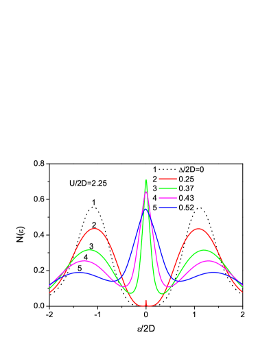
Figure 2: Density of states of Hubbard model at half-filling for different disorder levels $\Delta$ HubDis . (a) — correlated metal with $U=2.5D$. (b) — Mott insulator with $U=4.5D$. Temperature $T/2D$=0.0005.

In Fig. 2 we present our results HubDis for DMFT+$\Sigma$ densities of states for typical strongly correlated metal with $U=2.5D$, both in the absense of disorder and for different values of disorder scattering $\Delta$, including strong enough values of disorder, which transforms correlated metal to correlated Anderson insulator. In metallic phase disorder scattering leads to a typical broadening and suppression of the density of states.

Much more unusual is the the result obtained for $U=4.5D$, typical for Mott insulator phase and shown on Fig. 2(b). Here we observe the recovery of the central peak (quasiparticle band) in the density of states with the increase of disorder, transforming Mott insulator to correlated metal or to correlated Anderson insulator. Similar density of states behavior for disordered Hubbard model was reported also in Ref. BV , using direct numerical DMFT calculations in finite lattices.

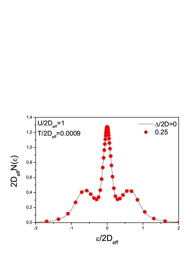
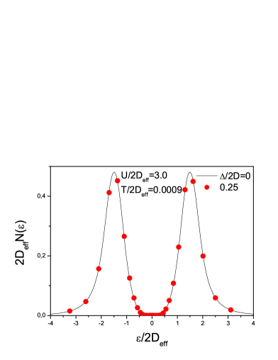
Figure 3: Universal dependence of properly normalized density of states on normalized energy $\varepsilon/2D_{eff}$ in Hubbard model for different disorder levels $\Delta$. (a) — correlated metal ($U/2D_{eff}$=1.0) with no disorder and for $\Delta/2D=$0.25. (b) — Mott insulator ($U/2D_{eff}$=3.0) without disorder and for $\Delta/2D=$0.25. Temperature $T/2D_{eff}$=0.0009.

Physical origin of such quite unexpected central peak restoration is evident. Controlling parameter of metal-insulator transition in DMFT is the ratio of Hubbard interaction $U$ to bare bandwidth $2D$. Introduction of disorder (in the absense of Hubbard interaction) leads to new effective bandwidth $2D_{eff}$ (cf. (11)), growing with disorder. This leads to diminishing values of the ratio $U/2D_{eff}$, which in its turn causes restoration of the quasiparticle band.

More so, in complete accordance with analytic arguments presented above, the density of states behavior in disordered Hubbard model with semi – elliptic actually demonstrates the universal dependence on disorder. This is clearly seen from Fig. 3, where we show properly normalized typical densities of states $2D_{eff}N(\varepsilon)$ in metallic (normalized interaction value $U/2D_{eff}$=1.0) and insulating phase (corresponding to $U/2D_{eff}$=3.0) without disorder and for the typical value of disorder scattering $\Delta/2D=$0.25. The densities of states in the absence and in the presence of disorder are actually described by the same (universal) dependences if expressed via properly normalized parameters.

In the absense of disorder one of the characteristic features of Mott-Hubbard metal-insulator transition is hysteresis behavior of the density of states, appearing with the decrease of $U$, starting from insulating phase georges96 ; Bull . Mott insulator phase remains (meta)stable down to rather small values of $U$ deep within the correlated metal phase and metallic phase is restored only at about $U_{c1}/2D\approx 1$. Corresponding interval of interaction parameter $U_{c1}<U<U_{c2}$ represents a coexistence region of metallic and Mott insulating phases, where, from a thermodynamic point of view, metallic phase is more stable georges96 ; Bull ; Blum . Such hysteresis in density of states behavior is observed also in the presence of disorder HubDis ; HubDis2 .

III.2 Optical conductivity: Mott-Hubbard and Anderson transitions

In the absence of disorder our calculations reproduce conventional DMFT results pruschke ; georges96 , with optical conductivity characterized by typical Drude peak at low frequencies and wide maximum at about $\omega\sim U$, which corresponds to optical transitions to the upper Hubbard band. As $U$ grows Drude peak is suppressed and disappears completely at Mott transition. Introduction of disorder leads to qualitative changes of the frequency dependence of optical conductivity.

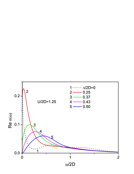
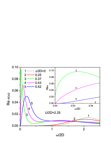
Figure 4: Real part of optical conductivity of Hubbard model at half-filling for different disorder levels $\Delta$ HubDis . (a) – typical correlated metal with $U=2.5D$. Curves 1,2, – metallic phase, curve 3 corresponds to the mobility edge (Anderson transition), curves 4,5 – correlated Anderson insulator. (b) – typical Mott insulator with $U=4.5D$. Curves 1,2 correspond to Mott insulator, curve 3 – mobility edge (Anderson transition), curves 4,5 – correlated Anderson insulator. Inset shows magnified low frequency region. Temperature $T/2D$=0.0005.

Fig. 4(a) shows the real part of optical conductivity of Hubbard model at half-filling for different disorder levels $\Delta$ and $U=2.5D$ typical for correlated metal. Transitions to the upper Hubbard bands at energies $\omega\sim U$ are almost unobservable. However it is clearly visible that metallic Drude peak typically centered at zero frequency is broadened and suppressed by disorder, gradually transforming into a peak at finite frequency because of Anderson localization effects. Anderson transition takes plase at $\Delta_{c}\approx 0.74D$ (corresponding to the curve 3 on all figures here). Notice that this value explicitly depends on value of the cutoff in the equation for the generalized diffusion coefficient, which is defined upto the coefficient of the order of unity MS83 ; Diagr . Naive expectations can lead to conclusion that narrow quasiparticle band at the Fermi level (formed in a strongly correlated metal) may be localized much more easily than the usual conduction band. However, these expectations are wrong and the band localizes only at rather large disorder $\Delta_{c}\sim D$ of the order of conduction band width $\sim 2D$. This is in qualitative agreement with the results for localization transition in two-band model ErkS .

In the DMFT+$\Sigma$ approach critical disorder value $\Delta_{c}$ does not depend on $U$ as interaction effects enter here only through $\Delta\Sigma^{RA}(\omega)\to 0$ for $\omega\to 0$ (for $T=0$, $\varepsilon=0$), so that the influence of interaction at $\omega=0$ just disappears. In fact this is the main shortcoming of DMFT+$\Sigma$ approach originating from the neglect of interference effect between interaction and impurity scattering. Significant role of these interference effects is actually well known for a long time Lee85 ; ma . However, the neglect of these effects allows us to perform the reasonable physical interpolation between two main limits – that of Anderson transition because of disorder and Mott-Hubbard transition because of strong correlations.

On Fig. 4(b) we show the real part of optical conductivity of Mott-Hubbard insulator with $U=4.5D$ for different disorder levels $\Delta$. In the inset we show low frequency data, demonstarting different types of conductivity behaviour, especially close to Anderson transition and within the Mott insulator phase. On the main part of the figure contribution to conductivity from transitions to upper Hubbard band at about $\omega\sim U$ is clearly seen. Disorder growth results in the appearance of finite conductivity for the frequencies inside Mott-Hubbard gap, correlating with the restoration of quasiparticle band in the density of states within the gap as shown in Fig. 2(b). This conductivity for $\Delta<\Delta_{c}$ is metallic (finite in the static limit $\omega=0$), and for $\Delta>\Delta_{c}$ at low frequencies we get ${\rm Re}\sigma(\omega)\sim\omega^{2}$, which is typical for Anderson insulator VW ; Diagr ; MS83 ; VW92 .

A bit unusual is the appearance in ${\rm Re}\sigma(\omega)$ of a peak at finite frequencies even in the metallic phase. This happens because of importance of localization effects. In the “ladder” approximation for $\Phi^{0RA}_{\varepsilon}(\omega,{\bf q})$ which neglects all localization effects we obtain the usual Drude peak at $\omega=0$ HubDis , while taking into account localization effects shifts the peak in ${\rm Re}\sigma(\omega)$ to finite frequencies.

Above we presented the data for conductivity data obtained for the case of increase of $U$ from metallic to Mott insulator phase. As $U$ decreases from Mott insulator phase we observe hysteresis of conductivity in coexistence region defined (in the absense of disorder) by inequality $U_{c1}<U<U_{c2}$. Hysteresis of conductivity is also observed in the coexistence region in the presence of disorder. More details can be found in Refs. HubDis ; HubDis2 .

In general, the picture of conductivity behavior obtained in DMFT+$\Sigma$ approximation is rather rich, demonstarting both Mott – Hubbard transition due to strong correlations and disorder induced Anderson (localization) transition. The complicate behavior under disordering is essentially determined by two – particle Green’s function behavior and does not shown a kind of universality, demonstrated above for the single – particle density of states.

III.3 Phase diagram of disordered Hubbard model at half-filling

Phase diagram of repulsive disordered Hubbard model at half-filling was studied in Ref. BV , using direct DMFT numerics for lattices with finite number of sites with random realizations of energies $\epsilon_{i}$ in (1), with subsequent averaging over many lattice realizations to obtain the averaged density of states and geometric mean local density of states, which allows to determine the critical disorder for Anderson transition. Below we present our results on disordered Hubbard model phase diagram obtained from density of states and optical conductivity calculations in DMFT+$\Sigma$ approach HubDis .

Figure 5: Phase diagram of disordered Hubbard model HubDis . Continuous curves are Mott insulator phase boundaries $U_{c1,c2}(\Delta)$ obtained from analytical estimate of Eq. (17), different symbols represent results for these boudaries obtained from calculations from density of states and optical conductivity. Line of Anderson transition is given by $\Delta_{c}=0.37$.

Calculated disorder – correlation strength $(\Delta,U)$ phase diagram at zero temperature is shown in Fig. 5 (actually calculations were performed at very low $T/2D$=0.0005). Anderson transition line $\Delta_{c}\approx 0.74D$ is defined as disorder strength for which static conductivity becomes zero at $T=0$. Mott-Hubbard transition can be detected either from central peak disappearance in the density of states or from optical conductivity by observation of gap closing in the insulating phase or from static conductivity disappearance in the metallic phase.

We have already noticed that DMFT+$\Sigma$ approximation gives universal ($U$ independent) value of critical disorder $\Delta_{c}$ because of neglect of interference between disorder scattering and Hubbard interaction. This leads to the difference between the phase diagram of Fig. 5 and the one obtained by numerical simulations in Ref. BV . At the same time the qualitative form of our phase diagram is highly nontrivial and qualitatively coincide with results of Ref. BV . Main difference is conservation of Hubbard bands in our results even in the limit of high enough disorder, while in the Ref. BV they just disappear. Phase coexistence region in Fig. 5 slowly widens with disorder growth instead of vanishing at some “critical” point as on phase diagram of Ref. BV . Coexistence boundaries (Mott insulator phase boundaries), obtained with decrease or increase of $U$, represented by curves $U_{c1}(\Delta)$ and $U_{c2}(\Delta)$ on Fig. 5, can actually be obtained from the simple equation:

$$\frac{U_{c1,c2}(\Delta)}{D_{eff}}=\frac{U_{c1,c2}}{D},$$ (16)

where effective bandwidth in the presence of disorder is calculated for $U=0$ within self-consistent Born approximation (4), (11). Thus the boundaries of coexistence region (which define also the boundaries of Mott insulator phase) are given by:

$$U_{c1,c2}(\Delta)=U_{c1,c2}\sqrt{1+4\frac{\Delta^{2}}{D^{2}}}$$ (17)

which are shown in Fig. 5 by dotted and solid lines. Phase transition points detected from disappearance of quasiparticle peak as well as points following from qualitative changes of conductivity behaviour are shown in Fig. 5 by different symbols. These symbols demonstrate very good agreement with analytical results confirming the choice of the ratio (16) as a controlling parameter of Mott transition in the presence of disorder. Thus, this transition is essentially controlled by simple band – widening effects due to disorder scattering, similarly to density of states behavior demonstrated above.

Note that the values of normalized density of states $2D_{eff}N(\varepsilon)$ are universal along each of these boundaries, as well as along any curve in ($\Delta$,$U$) – plane, determined by the equation:

$$U(\Delta)=U(0)\sqrt{1+4\frac{\Delta^{2}}{D^{2}}}$$ (18)

in accordance with our discussion on the universal dependence of the densities of states on disorder presented above.

Essentially similar results were obtained for the density of states behavior, dynamic conductivity and phase diagram HubDis2 in the case of the conduction band with “flat” density of states in the absence of disorder and interactions, which qualitatively corresponds to the two – dimensional case. This is not surprising, as both large enough disorder and interactions transform the “flat” band into a kind of smeared semi – elliptic band. Some explicit examples of this kind of behavior will be presented below for the case of attractive Hubbard model.

IV Attractive Hubbard model with disorder

The studies of superconductivity in BCS – BEC crossover region attracts theorists for rather long time Leggett and most important advance here was made by Nozieres and Schmitt-Rink NS , who proposed an effective approach to describe $T_{c}$ crossover. Attractive Hubbard model is probably the simplest model allowing theoretical studies of BCS-BEC crossover NS . This model was studied within DMFT in a number of recent papers Keller01 ; Toschi04 ; Bauer09 ; Koga11 . However only few results were obtained for the normal (non-superconducting) phase of this model, especially in disordered case. Similarly, there were practically no studies of two – particle properties, such as optical conductivity. Below we present a summary of our results obtained within DMFT+$\Sigma$ approach and make comparison with similar results for repulsive Hubbard model.

IV.1 Density of states and optical conductivity

In the special case of half – filled band ($n=1$) the densities of states of attractive and repulsive Hubbard models just coincide (due to exact mapping of these models onto each other). Thus, below we discuss the more typical case of quarter – filled band ($n=0.5$). In Fig. 6 we show densities of states obtained for $T/2D=0.05$ for different values of attractive interaction ($U<0$). Fig. 6(a) should be compared with Fig. 6(b), where we present similar results for repulsive ($U>0$) case. We can see that the densities of states close to the Fermi level drop with the growth of $U$, both for attraction (Fig. 6(a)) and repulsion (Fig. 6(b)), but significant growth of $|U|$ in repulsive case leads only to vanishing quasiparticle peak, so that the density of states at the Fermi level becomes practically independent of $U$, while in attractive case the growth of $|U|$ leads to superconducting pseudogap opening at the Fermi level (curves 5, 6 in Fig. 6(a)) and for $|U|/2D>1.2$ we observe the full gap opening at the Fermi level (curves 7-9 in Fig. 6(a)). This gap is not directly related to the emergence of superconducting state, but is due to the appearance of preformed Cooper pairs at the temperatures larger than superconducting transition temperature (which is lower, than the temperature $T/2D=0.05$ used in our calculations). Here we actually observe the important difference between attractive and repulsive cases — in case of repulsion deviation from half – filling leads to metallic state for arbitrary values of $U$ and insulating gap at large $U$ opens not at the Fermi level.

This picture of density of states evolution with the growth of $|U|$ is also supported by the behavior of optical conductivity shown in Fig. 7. We see that the growth of $|U|$ leads to the replacement of Drude peak at zero frequency (curves 1-3 in Fig. 7) by pseudogap dip (curves 5, 6 in Fig. 7) and wide maximum of conductivity at finite frequency, connected with transitions across the pseudogap. The further increase of $|U|$ leads to opening of the full gap in optical conductivity due to formation of Cooper pairs (curves 7-9 in Fig. 7).

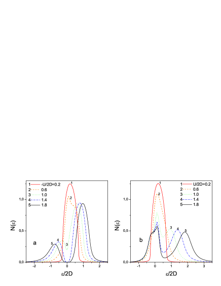
Figure 6: Densities of states and for different values of Hubbard attraction (a) and repulsion (b). Temperature $T/2D=0.05$.

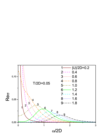
Figure 7: Optical conductivity for different values of attractive Hubbard attraction. Temperature $T/2D=0.05$.

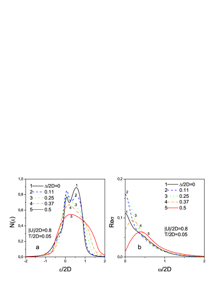
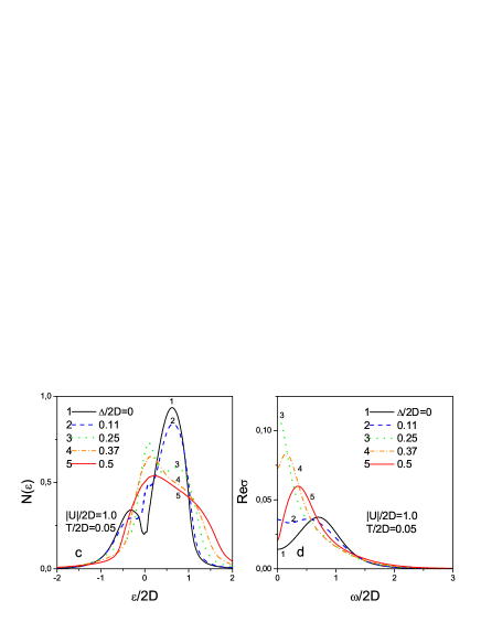
Figure 8: Evolution of the density of states (left panels) and optical conductivity (right panels) with disorder for different values of $U$ ($|U|/2D=0.8$ - (a),(b); $|U|/2D=1$ - (c),(d); $|U|/2D=1.6$ - (e),(f)).

In Fig. 8 we present the evolution of the density of states and optical conductivity with changing disorder. At weak enough attraction ($|U|/2D=0.8$, Fig. 8(a),(b)), the growth of disorder just widens the density of states. Disorder effectively masks peculiarities of the density of states due to correlation effects. In particular, quasiparticle peak and the “wings” due to upper and lower Hubbard bands present in Fig. 8(a) in the absence of disorder completely vanish at strong enough disorder. Evolution of optical conductivity with the growth of disorder $\Delta$, shown in Fig. 8(b), is in general agreement with the evolution of density of states. Weak enough disordering (curves 1-3 in Fig. 8(b)), leads to some growth of static conductivity, which is connected with suppression of correlation effects at the Fermi level (curves 1-3 in Fig. 8(a). The further growth of disorder leads to significant widening of the band and the drop of the density of states (curve 5 in Fig. 8(a),(b)), which leads to the drop of static conductivity. Finally, the growth of disorder leads to Anderson localization which takes place at $\Delta/2D=0.37$ for $T=0$ HubDis . However, here we consider the case of high enough temperature $T/2D=0.05$, so that static conductivity (see curves 6, 7 in Fig. 8(b)) always remains finite, though the localization behavior is also clearly seen and $\sigma(\omega)\sim\omega^{2}$. At larger value of attractive interaction $|U|/2D=1$ the evolution of the density of states and optical conductivity is more or less similar (Fig. 8(c),(d) ). However, in the absence of disorder we observe here Cooper pairing pseudogap in the density of states, while disorder leads to its suppression, leading both to the growth of the density of states at the Fermi level and related growth of static conductivity. Finally, at still larger attraction $|U|/2D=1.6$ (Fig. 8(e),(f)) in the absence of disorder there is the real Cooper pairing gap in the density of states. This gap is also evident in optical conductivity. With the growth of disorder Cooper pairing gap both in the density of states and conductivity becomes narrower (curves 2-5). Further growth of disorder leads to complete suppression of this gap and restoration of metallic state with finite density of states at the Fermi level and finite static conductivity. This closure of Cooper gap is obviously related to the effective growth of the conduction bandwidth $2D_{eff}$, which leads to the lowering of $|U|/2D_{eff}$ ratio, which actually controls the formation of Cooper gap. Situation here is similar to the closure of Mott gap by disorder in repulsive Hubbard model discussed above HubDis . However, at large disorder (curve 7 in Fig. 8(f)) we clearly observe localization behavior, so that the growth of disorder at $T=0$ will first lead to metallic state (the closure of Cooper pairing gap), while the further growth of disorder will induce Anderson metal – insulator transition. Similar picture is observed for large positive $U$ at half-filling ($n=1$) HubDis , where the growth of disorder leads to Mott insulator – correlated metal – Anderson insulator transition.

Let us now demonstrate the universality of disorder dependence of the density of states as an example of the most important single – particle property. Let us concentrate on the most typical case of the density of states evolution shown in Fig. 8 (a). We can easily convince ourselves, that this evolution is only due to the general widening of the band due to disorder (cf. (11)), as all the data for the density of states fit the same universal curve replotted in appropriate new variables, with all energies (and temperature) normalized by the effective bandwidth by replacing $D\rightarrow D_{eff}$, as shown in Fig. 9(a), in complete accordance with results obtained above in repulsive Hubbard model for semi – ellipric band.

In the case of initial (“bare”) conduction band with flat density of states, there is no complete universality, as is seen from Fig. 9(b) for low enough values of disorder. However, for large enough disorders the dashed curve in Fig. 9(b) practically coincides with universal curve for the density of states shown in Fig. 9(a). This reflects the simple fact, that at large enough disorders the flat density of states is effectively transformed into semi – elliptic oneJETP15 .

Figure 9: Universal dependence of the density of states on disorder in attractive Hubbard model: (a) — the model of semi – elliptic “bare” density of states. (b) — the model of flat “bare” density of states.

IV.2 Generalized Anderson theorem

Superconducting transition temperature $T_{c}$ in general is not a single – particle characteristic of the system. Cooper instability, determining $T_{c}$ is related to divergence of two – particle loop in Cooper channel. In the weak coupling limit, when superconductivity is due to the appearance of Cooper pairs at $T_{c}$, disorder only slightly influences superconductivity with $s$-wave pairing SCLoc ; Genn . This is the essence of the so called Anderson theorem and changes of $T_{c}$ are due only to the relatively small changes of the density of states at the Fermi level induced by disorder.

In region of BCS – BEC crossover and in the strong coupling region Nozieres – Schmitt-Rink approach NS assumes, that corrections due to strong pairing attraction significantly change the chemical potential of the system, while possible correction due to this interaction to Cooper instability condition can be neglected, so that we can always use the weak coupling (ladder) approximation. Then the condition of Cooper instability in disordered Hubbard model takes the form:

$$1=-|U|\chi_{0}(q=0,\omega_{m}=0)$$ (19)

where

$$\chi_{0}(q=0,\omega_{m}=0)=-T\sum_{n}\sum_{\bf pp^{\prime}}\Phi_{\bf pp^{\prime}}(\varepsilon_{n})$$ (20)

represents the two – particle loop (susceptibility) in Cooper channel “dressed” only by disorder scattering, and $\Phi_{\bf pp^{\prime}}(\varepsilon_{n})$ is the averaged two – particle Green’s function in Cooper channel ($\omega_{m}=2\pi mT$ and $\varepsilon_{n}=\pi T(2n+1)$ are the usual Boson and Fermion Matsubara frequencies).

Using the exact Ward identity, derived in Ref. PRB07

$$G(\varepsilon_{n},{\bf p})-G(-\varepsilon_{n},-{\bf p})=$$

$$=-\sum_{\bf p^{\prime}}\Phi_{\bf pp^{\prime}}(\varepsilon_{n})(G_{0}^{-1}(\varepsilon_{n},{\bf p^{\prime}})-G_{0}^{-1}(-\varepsilon_{n},-{\bf p^{\prime}})),$$

(21)

where $G(\varepsilon_{n},{\bf p})$ is the impurity averaged (but not containing Hubbard interaction corrections!) single – particle Green’s function, we can show JETP15 that Cooper susceptibility (20) is given by:

$$\chi_{0}(q=0,\omega_{m}=0)=$$

$$=T\sum_{n}\frac{\sum_{\bf p}G(\varepsilon_{n},{\bf p})-\sum_{\bf p}G(-\varepsilon_{n},{\bf p})}{2i\varepsilon_{n}}=$$

$$=T\sum_{n}\frac{\sum_{\bf p}G(\varepsilon_{n},{\bf p})}{i\varepsilon_{n}}.$$ (22)

After the standard summation over Matsubara frequencies Diagr we get:

$$\chi_{0}(q=0,\omega_{m}=0)=$$

$$=\frac{1}{4\pi i}\int_{-\infty}^{\infty}d\varepsilon\frac{\sum_{\bf p}G^{R}(\varepsilon,{\bf p})-\sum_{\bf p}G^{A}(\varepsilon,{\bf p})}{\varepsilon}th\frac{\varepsilon}{2T}$$

$$=-\int_{-\infty}^{\infty}d\varepsilon\frac{\tilde{N}_{0}(\varepsilon)}{2\varepsilon}th\frac{\varepsilon}{2T},$$ (23)

where $\tilde{N}_{0}(\varepsilon)$ is the density of states ($U=0$) renormalized by disorder scattering. In Eq. (23) the energy $\varepsilon$ origin is at the chemical potential. If the origin of energy is shifted to the middle of conduction band we have to replace $\varepsilon\to\varepsilon-\mu$, and the condition of Cooper instability (19) leads to the following equation for $T_{c}$:

$$1=\frac{|U|}{2}\int_{-\infty}^{\infty}d\varepsilon\tilde{N}_{0}(\varepsilon)\frac{th\frac{\varepsilon-\mu}{2T_{c}}}{\varepsilon-\mu},$$ (24)

The chemical potential of the system at different values of $U$ and $\Delta$ now should be determined from DMFT+$\Sigma$ calculations, i.e. from the standard equation for the number of electrons (band-filling), determined by Green’s function given by Eq. (3), which allows us to find $T_{c}$ for the wide range of model parameters, including the BCS-BEC crossover and strong coupling regions, as well as for different levels of disorder. This is the gist of Nozieres – Schmitt-Rink approximation — in the weak coupling region superconducting transition temperature is controlled by the equation for Cooper instability (24), while in the strong coupling limit it is determined by the temperature of Bose – Einstein condensation, which is controlled by chemical potential. Then the joint solution of Eq. (24) and equation for the chemical potential guarantees the correct interpolation for $T_{c}$ through the region of BCS-BEC crossover. In the absence of disorder this combination of Nozieres – Schmtt-Rink approximation with DMFT produces the results for the critical temperature, which, as shown in Fig. 10, are almost quantitatively close to exact results, obtained by direct numerical DMFT calculations Keller01 ; Toschi04 ; Koga11 ; JETP14 , but demands much less numerical efforts.

Eq. (24) demonstrates, that Cooper instability depends on disorder only through the disorder dependence of the density of states $\tilde{N}_{0}(\varepsilon)$, which is the main statement of Anderson theorem. Within Nozieres – Schmitt-Rink approach Eq. (24) is conserved also in the region of strong coupling, when the critical temperature is determined by BEC condition for compact Cooper pairs. However, the chemical potential $\mu$, entering Eq. (24), may significantly depend on disorder. In DMFT+$\Sigma$ approximation this dependence of chemical potential (as well as any other single – particle characteristic) in the model with semi – elliptic density of states is only due to disorder widening of conduction band. In this sence both in BCS – BEC crossover region and in the strong coupling limit a kind of generalized Anderson theorem actually holds and Eq. (24) leads to universal dependence of $T_{c}$ on disorder, due to the change of $D\to D_{eff}$. Such universality is fully confirmed by direct numerical calculations of $T_{c}$ in this model, performed in Ref. JTL14 .

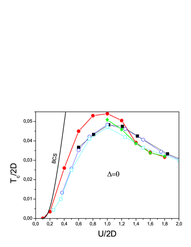
Figure 10: Dependence of superconducting critical temperature on attractive interaction strength. Black squares, white circles and white squares show the results of Refs. Keller01 ,Toschi04 ,Koga11 respectively for quarter-filled band with $n=0.5$. Stars represent the results obtained numerically from the criterion of instability of the normal phase in Ref. JETP14 . Filled circles show $T_{c}$ in Nozieres – Schmitt-Rink approximations, combined with DMFT JETP14 . Continuous black curve represents the result of BCS theory.

Figure 11: Dependence of superconducting transition temperature on disorder for different values of Hubbard attraction $U$: (a) — semi – elliptic band. (b) — flat band.

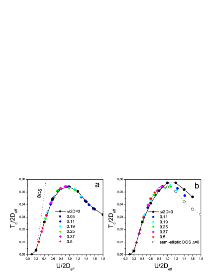
Figure 12: Universal dependence of superconducting critical temperature on Hubbard attraction $U$ for different disorder levels: (a) — semi – elliptic band. Dashed curve represent BCS dependence in the absence of disorder. (b) — flat band. Dashed line represents similar dependence for semi – elliptic band for $\Delta=0$.

In Fig. 11 we present the dependence of $T_{c}$ (normalized by the critical temperature in the absence of disorder $T_{c0}=T_{c}(\Delta=0$)) on disorder for different values of pairing interaction $U$ for both models of initial semi – elliptic density of states (Fig. 11(a)) and for the case of flat density of states (Fig. 11(b)). Qualitatively the evolution of $T_{c}$ with disorder is the same for both models. In the weak coupling limit ($U/2D\ll 1$) disorder slightly suppresses $T_{c}$ (curves 1). At intermediate couplings ($U/2D\sim 1$) weak disorder increases $T_{c}$, while the further growth of disorder suppresses the critical temperature (curves 3). In the strong coupling region ($U/2D\gg 1$) the growth of disorder leads to significant increase of the critical temperature (curves 4,5). However, this rather complicate dependence of $T_{c}$ on disorder is actually completely determined simply by disorder widening of the initial ($U=0$) conduction band, demonstrating the validity of the generalized Anderson theorem for all values of $U$. In Fig. 12 curve with octagons show the dependence of the critical temperature $T_{c}/2D$ on coupling strength $U/2D$ in the absence of disorder ($\Delta=0$) for both models of initial conduction bands (semi – elliptic — Fig. 12(a) and flat — Fig. 12(b)). In both models in the weak coupling region superconducting transition temperature is well described by BCS model (in Fig. 12(a) the dashed curve represents the result of the solution of BCS model, with $T_{c}$ determined by Eq. (24), with chemical potential independent of $U$ and determined by quarter – filling of the “bare” band), while in the strong coupling region the critical temperature is determined by Bose – Einstein condesation of Cooper pairs and drops as $t^{2}/U$ with the growth of $U$ (inversely proportional to the effective mass of the pair), passing through the maximum - at $U/2D_{eff}\sim 1$. The other symbols in Fig. 12(a) show the results for $T_{c}$ obtained by combination of DMFT+$\Sigma$ and Nozieres – Schmitt-Rink approximations for the case of semi – elliptic band. We can see, that all data (expressed in normalized units of $U/2D_{eff}$ and $T_{c}/2D_{eff}$) ideally fit the universal curve, obtained in the absence of disorder. For the case of flat band, results of our calculations are shown in Fig. 12(b) and we do not observe the complete universality — data points, corresponding to different degrees of disorder slightly deviate from the curve, obtained in the absence of disorder. However, with the growth of disorder the flat density of states gradually transforms to semi – elliptic and our data points move towards the universal curve, obtained for semi – elliptic case and shown by the dashed curve in Fig. 12(b), confirming the validity of the generalized Anderson theorem also in this case.

IV.3 Ginzburg – Landau coefficients

Universal dependence on disorder is also observed for the coefficients of Ginzburg – Landau expansion $A$ (homogeneous quadratic term of the expansion) and $B$ (fourth-order term), related to Cooper – channel vertices with the sum of incoming (outgoing) momenta $q=0$. Coefficient $A$ is given by Diagr :

$$A(T)=\chi_{0}(q=0,T)-\chi_{0}(q=0,T_{c}),$$ (25)

where $\chi_{0}(q=0,T)$ is Cooper susceptibility (20), and subtraction of $\chi_{0}(q=0,T_{c})$ guarantees the zero value of $A(T=T_{c})$. Using (19) to determine $\chi_{0}(q=0,T_{c})$ and (23) for $\chi_{0}(q=0,T)$, we get:

$$A(T)=\frac{1}{|U|}-\int_{-\infty}^{\infty}d\varepsilon\tilde{N}_{0}(\varepsilon)\frac{th\frac{\varepsilon-\mu}{2T}}{2(\varepsilon-\mu)}.$$ (26)

so that the coefficient $A(T)$ reduces to zero for $T\to T_{c}$, and is written as:

$$A(T)=a(T-T_{c}).$$ (27)

For the case of “bare” band with semi – elliptic density of states the dependence of $a$ on disorder is related only to the general widening of the band by disorder, i.e. is completely described by the replacement $D\to D_{eff}$. Thus, in the presence of disorder we obtain the universal dependence of $a$ on $U$ (normalized by $D_{eff}$), shown in Fig. 13a.

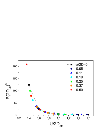
Figure 13: Universal dependence of Ginzburg – Landau coefficients $a$ (a) and $B$ (b) on Hubbard attraction for different disorder levels. Dotted line with black squares shows the case of $\Delta=0$.

Ginzburg – Landau coefficient $B$ is determined by the “loop” diagramm with four Cooper vertices Diagr . After rather complicated analysis, to be presented elsewhere, which is based on some generalizations of Ward identity (21), it can be shown exactly, that $B$ is given by:

$$B=\int_{-\infty}^{\infty}\frac{d\varepsilon}{4(\varepsilon-\mu)^{3}}\left(th\frac{\varepsilon-\mu}{2T}-\frac{(\varepsilon-\mu)/2T}{ch^{2}\frac{\varepsilon-\mu}{2T}}\right)\tilde{N}_{0}(\varepsilon)$$ (28)

Thus, the dependence of coefficient $B$ on disorder, similarly to $A$, is determined only by the density of states $\tilde{N}_{0}(\varepsilon)$ renormalized (widened) by disorder and the chemical potential $\mu$. Then, in the case of semi – elliptic density of states the dependence of $B$ on disorder is reduced to the simple replacement $D\to D_{eff}$, so that in the presence of disorder we obtain again the universal dependence of $B$ on $U$, shown in Fig. 13b.

It should be noted that Eqs. (26) and (28) for coefficients $A$ and $B$ were otained using the exact Ward identities and remain valid also in the limit of strong disorder (Anderson localized phase), when both. $A$ and $B$ depend on disorder also only via the effective bandwidth $D_{eff}$.

This universal dependence on disorder (due only to the replacement $D\to D_{eff}$) is reflected also in the specific heat discontinuity at the transitio temperature, which is determined by coefficients $a$ and $B$:

$$C_{s}(T_{c})-C_{n}(T_{c})=T_{c}\frac{a^{2}}{B}$$ (29)

To determine the coefficient $C$ in gradient term of Ginzburg – Landau expansion we need the knowledge of nontrivial of $q$-dependence of Cooper vertex Diagr , which is essentially changed by disorder scattering. In particular, the behavior of coefficient $C$ is qualitatively changed at Anderson localization transition SCLoc . Thus, the coefficient $C$ is basically determined by two – particle charateristics of the system and does not demopnstrate the universal dependence on disorder due only to changes of the effective bandwidth.

IV.4 Number of local pairs

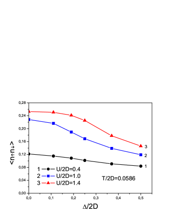
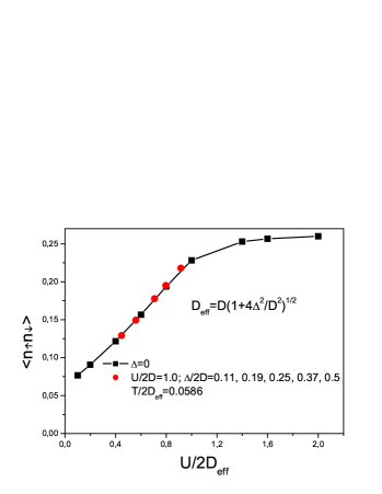
Figure 14: Dependence of the number of local pairs on disorder for different values of Hubbard attraction (a) and universal dependence on disorder, expressed via normalized variables at fixed value of $U/2D=1$ (b).

Disorder in attractive Hubbard model also leads to the suppression of the number of local pairs (doubly occupied sites). The average number of local pairs is determined by local (single site) pair correlation function $<n_{\uparrow}n_{\downarrow}>$, which in the absence of disorder grows with the increase of Hubbard attraction $U$ from $<n_{\uparrow}n_{\downarrow}>=<n_{\uparrow}><n_{\uparrow}>=n^{2}/4$ for $U/2D_{eff}\ll 1$ to $<n_{\uparrow}n_{\downarrow}>=n/2$ for $U/2D_{eff}\gg 1$, when all electrons become paired. In our calculations $n$=0.5 (quarter – filled band), so that $n/2$=0.25, while $n^{2}/4$=0.0625. The growth of $D_{eff}$ with disorder leads to an effective suppression of the parameter $U/2D_{eff}$ and corresponding suppression of the number of doubly occupied sites. In Fig. 14(a) we show the disorder dependence of the number of doubly occupied sites for three different values of Hubbard attraction. In all cases the growth of disorder suppresses the number of doubly occupied sites (local pairs). Similarly to $T_{c}$, the change of the number of local pairs with disorder can be attributed only to the change of the effective bandwidth (11) with the growth of disorder. In Fig. 14(b) the curve with black squares shows the dependence of the number of doubly occupied sites on attractive interaction in the absence of disorder at temperature $T/2D=0.0586$. This curve is actually universal — the dependence of the number of local pairs $<n_{\uparrow}n_{\downarrow}>$ on the scaled parameter $U/2D_{eff}$ with appropriately scaled temperature $T/2D_{eff}=0.0586$ in the presence of disorder is given by the same curve, which is shown by by circles representing data obtained for five different disorder levels, shown in Fig. 14(b) for the case of $U/2D=1$.

V Conclusion

In this paper, in the framework of DMFT+$\Sigma$ generalization of dynamical mean field theory UFN12 , we have studied and compared disorder effects in both repulsive and attractive Hubbard models. We examined both the problem of Mott – Hubbard and Anderson metal-insulator transitions in repulsive case, and BCS-BEC crossover region of attractive Hubbard model. We also performed extensive calculations of the densities of states and dynamic (optical) coductivity for the wide range of ineractions $U$ and at different disorder levels $\Delta$, demonstrating similarities and dissimilarities between repulsive and attractive cases.

We have shown analytically for the case of conduction band with semi – elliptic density of states (which is a good approximation for three – dimensional case) in DMFT+$\Sigma$ approximation disorder influences all single – particle properties (e.g. density of states) in a universal way — all changes of these properties are due only to disorder widening of the conduction band. In the model of conduction band with flat density of states (which is more appropriate for two – dimensional systems), there is no such universality in the region of weak disorder. However, the main effects are again due to general widening of the band and complete universality is restored for high enough disorders, when the density of states effectively becomes semi – elliptic. Similar universal dependences on disorder are also reflected in the phase diagram of repulsive Hubbard model and in superconducting critical temperature of attractive Hubbard model, where the combination of DMFT+$\Sigma$ and Nozieres – Schmitt-Rink approximations demonstrates the validity of the generalized Anderson theorem both in BCS – BEC crossover and strong coupling regions.

Naturally, no universal dependences on disorder were obtained for the two – particle properties like optical conductivity, where vertex corrections due to disorder scattering become very important, leading to new physics, like that of Anderson transition.

Overall, the use of DMFT+$\Sigma$ approximation to analyze the disorder effects in Hubbard model was shown to produce reasonable results for the phase diagram for repulsive case, as compared to exact numerical simulations of disorder in DMFT, density of states behavior and optical conductivity in both repulsive and attractive cases. However, the role of approximations made in DMFT+$\Sigma$, such as the neglect of the interference of disorder scattering and correlation effects, deserves further studies.

V.1 Acknowledgements

It is a pleasure and honour to dedicate this short review to Professor Leonid Keldysh 85-th anniversary. This work is supported by RSF grant No. 14-12-00502.

References

- (1) N.F. Mott. Metal - Insulator Transitions, 2nd edn. Taylor and Francis, London, 1990
- (2) J. Hubbard. Proc. Roy. Soc. London Ser. A 276, 238 (1963); Proc. Roy. Soc. London Ser. A 277, 237 (1964); Proc. Roy. Soc. London Ser. A 281, 401 (1964); Proc. Roy. Soc. London Ser. A 285, 542 (1965); Proc. Roy. Soc. London Ser. A 296, 829 (1967); Proc. Roy. Soc. London Ser. A 296, 100 (1967)
- (3) W. Metzner, D. Vollhardt. Phys. Rev. Lett. 62, 324 (1989)
- (4) D. Vollhardt in Correlated Electron Systems (Ed. by V.J. Emery). World Scientific, Singapore, 1993, p. 57
- (5) Th. Pruschke, M. Jarrell, J.K. Freericks Adv. Phys. 44, 210 (1995)
- (6) A. Georges, G. Kotliar, W. Krauth, M.J. Rozenberg. Rev. Mod. Phys. 68, 13 (1996)
- (7) D. Vollhardt. AIP Conference Proceedings 1297, 339 (2010); ArXiv:1004.5069
- (8) G. Kotliar, D. Vollhardt. Physics Today 57, 53 (2004)
- (9) D.M. Eagles. Phys. Rev. 186, 456 (1969)
- (10) A. J. Leggett, in Modern Trends in the Theory of Condensed Matter, edited by A. Pekalski and J. Przystawa (Springer, Berlin 1980).
- (11) P. Nozieres and S. Schmitt-Rink, J. Low Temp. Phys. 59, 195 (1985)
- (12) I. Bloch, J. Dalibard, and W. Zwerger. Rev. Mod. Phys. 80, 885 (2008)
- (13) L.P. Pitaevskii. Usp. Fiz. Nauk 176, 345 (2006) [Physics Uspekhi 44, 333 (2006)]
- (14) E.Z. Kuchinskii, I.A. Nekrasov, M.V. Sadovskii. Pis’ma Zh. Eksp. Teor. Fiz. 82, 217 (2005) [JETP Lett. 82 198 (2005)]
- (15) M.V. Sadovskii, I.A. Nekrasov, E.Z. Kuchinskii, Th. Prushke,V.I. Anisimov. Phys. Rev. B 72, 155105 (2005)
- (16) E.Z. Kuchinskii, I.A. Nekrasov, M.V. Sadovskii. 32, 528-537 (2006) [Low Temp. Phys. 32, 398 (2006)]
- (17) E.Z. Kuchinskii, I.A. Nekrasov, M.V. Sadovskii. Usp. Fiz. Nauk 182, 345-378 (2012) [Physics Uspekhi 55, 325 (2012)]
- (18) E.Z. Kuchinskii, I.A. Nekrasov, M.V. Sadovskii. Zh. Eksp. Teor. Fiz. 133, 670 (2008) [JETP 106, 581 (2008)]
- (19) E.Z.Kuchinskii, N.A.Kuleeva, I.A.Nekrasov, M.V.Sadovskii. Zh. Eksp. Teor. Fiz. 137, 368 (2010) [JETP 110, 325 (2010)]
- (20) E.Z.Kuchinskii, I.A.Nekrasov, M.V.Sadovskii. Phys. Rev. B 80, 115124 (2009)
- (21) E.Z. Kuchinskii, I.A. Nekrasov, M.V. Sadovskii. Phys. Rev. B 75, 115102 (2007)
- (22) N.A. Kuleeva, E.Z. Kuchinskii, M.V. Sadovskii. Zh. Eksp. Teor. Fiz. 146, 304 (2014) [JETP 119, 264 (2014)]
- (23) E.Z. Kuchinskii, N.A. Kuleeva, M.V. Sadovskii. Pis’ma Zh. Eksp. Teor. Fiz. 100, No. 3, 213 (2014) [JETP Lett. 100, No. 3, 192 (2014)]
- (24) E.Z. Kuchinskii, N.A. Kuleeva, M.V. Sadovskii. Zh. Eksp. Teor. Fiz. 147, No. 6 (2015) [JETP 120, No. 6 (2015)]; ArXiv:1411.1547
- (25) P.W. Anderson. Phys. Rev. 109, 1492 (1958)
- (26) M.V. Sadovskii. Diagrammatics (Singapore: World Scientific, 2006)
- (27) R. Bulla, T.A. Costi, T. Pruschke, Rev. Mod. Phys. 60, 395 (2008).
- (28) D. Vollhardt and P. Wölfle. Phys. Rev. B 22, 4666-4679 (1980); Phys. Rev. Lett. 48, 699 (1982); in Anderson Localization, eds. Y. Nagaoka and H. Fukuyama, Springer Series in Solis State Sciences, vol. 39, p.26. Springer Verlag, Berlin 1982.
- (29) M.V. Sadovskii. The Theory of Electron Localization in Disordered Systems. Soviet Scientific Reviews – Physics Reviews, ed. I.M. Khalatnikov, vol. 7, p.1. Harwood Academic Publ., NY 1986; A.V. Myasnikov., M.V. Sadovskii. Fiz. Tverd. Tela 24, 3569 (1982) [Sov. Phys.-Solid State 24, 2033 (1982) ]; E.A. Kotov, M.V. Sadovskii. Zs. Phys. B 51, No 1, 17 (1983)
- (30) P. Wölfle, D. Vollhardt in Electronic Phase Transitions, (Eds W. Hanke, Yu.V. Kopaev) (Amsterdam:North–Holland, 1992) 32 p. 1
- (31) K. Byczuk, W. Hofstetter, D. Vollhardt. Phys. Rev. Lett. 94, 056404 (2005)
- (32) R. Bulla. Phys. Rev. Lett. 83, 136 (1999); R. Bulla, T.A. Costi, D. Vollhardt. Phys. Rev. B 64, 045103 (2001)
- (33) N. Blümer. Mott–Hubbard Metal–Insulator Transition and Optical Conductivity. Thesis, München 2002.
- (34) P.A. Lee, T.V. Ramakrishnan. Rev. Mod. Phys. 57, 287 (1985); D. Belitz, T.R. Kirkpatrick. Rev. Mod. Phys. 66, 261 (1994)
- (35) A.M. Finkelshtein. Zh. Eksp. Teor. Fiz. 84 168 (1983) [Sov. Phys. JEPT 57 97 (1983)]; C. Castellani et al. Phys. Rev. B 30 527 (1984)
- (36) M.A. Erkabaev, M.V. Sadovskii M V. J. Moscow Phys. Soc. 2, 233 (1992)
- (37) M. Keller, W. Metzner, and U. Schollwock. Phys. Rev. Lett. 86, 4612 4615 (2001)
- (38) A. Toschi, P. Barone, M. Capone, and C. Castellani. New Journal of Physics 7, 7 (2005)
- (39) J. Bauer, A.C. Hewson, and N. Dupis. Phys. Rev. B 79, 214518 (2009)
- (40) A. Koga and P. Werner. Phys. Rev. A 84, 023638 (2011)
- (41) M.V. Sadovskii. Superconductivity and Localization. World Scientific, Singapore 2000
- (42) P.G. De Gennes. Superconductivity of Metals and Alloys. W.A. Benjamin, NY 1966