Interference-Cooperation in Multi-User/Multi-Operator Receivers

Abstract

In a multi-user scenario where users belong to different operators, any interference mitigation method needs unavoidably some degree of cooperation among service providers. In this paper we propose a cooperation strategy based on the exchange of mutual interference among operators, rather than of decoded data, to let every operator to recover an augmented degree of diversity either for channel estimation and multi-user detection. In xDSL scenario where multiple operators share the same cable binder the interference-cooperation (IC) approach outperforms data-exchange methods and preserves to certain degree the privacy of the users as signals can be tailored to prevent each operator to infer parameters (channel and data) of the users from the other operators.

The IC method is based on Expectation Maximization estimation shaped to account for the degree of information that each operator can exchange with the others during the two steps of multi-user channel estimation and multi-user detection. Convergence of IC is guaranteed into few iterations and it does not depend on the structure of the interference. IC performance attains those of centralized receivers (i.e., one fusion-center that collects all the received signals from all the users/operators), with some loss when in heavily interfered multi-user channel such as in twisted-pair communications allocated beyond 50-100MHz spectrum.

I Introduction

Interference mitigation is a largely investigated topic in communication systems for wired and wireless technology. The increasing demand of data-intensive services in fixed and mobile communication brings new challenges for interference cancellation, and service providers (SPs) are looking for solutions that not only meet current, but mostly future requirements, still preserving the downward compatibility.

Existing copper-wire infrastructure to provide net-bidirectional data rate of up to 200Mbps can use short loop lengths and high frequencies as in ITU-T G.993.2 recommendation [1]. Single cable binder can contain up to hundreds twisted pairs and these can be shared by multiple coexisting SPs. In multi-pair cable, crosstalk is the dominant impairment caused by the capacitive and inductive coupling among the twisted pairs. Techniques have been proposed to mitigate near-end crosstalk (NEXT) such as spectral shaping and frequency division duplexing [2], [3]. However, in digital subscriber line (DSL) the data rate is still limited by the far-end crosstalk (FEXT) that can be mitigated only by appropriate interference cancellation methods. More specifically, the performance is improved by using multi-user processing for FEXT cancellation, or vectoring [4]. DSL Access Multiplexer (DSLAM) hosts signal processing units to mitigate upstream FEXT generated within a vectored group belonging to the same SP. In common DSL scenario, non-vectored lines coexist along with the vectored groups in a same cable binder, and this prevents reliable FEXT control. Referring to multi-operator scenario in Fig.1, vectoring technique is very efficient to cancel self-FEXT (i.e., FEXT of the same SP), but it has no control of FEXT due to the non-vectored lines and from other vectored group in the same cable binder (so called alien-FEXT) when twisted-pairs are shared among non-cooperating SPs. This problem is even more challenging in next generation G.Fast standard where the bandwidth is even larger than 100MHz [5] over 50-200m cable length and alien-FEXT induced from just one temporary line-mismatch could loose all the benefits of vectoring at the expenses of energy [6].

In this scenario, centralized vectoring where FEXT mitigation is controlled by one single processing unit for multiple SPs would be beneficial but it is unfeasible due to the regulations of physical unbundling [7]. In addition, due to the privacy issue, SPs are not prone to exchange each other data to ease interference cancellation, even if in turn from this exchange there would be a benefit for all. Dynamic spectrum management methods could provide the same benefit as vectored transmission in the mix vectored and non-vectored (or equivalently non-cooperating SPs) cable environment [8]. Noise decorrelation technique can handle alien-FEXT as additive structured noise, at the price of additional initialization (to estimate noise correlation) and adaptation (for time varying alien-FEXT scenario) algorithms [9]. If in vectored groups the non-vectored lines are unmanaged, the benefits of vectoring degrade rapidly [10]. The way to handle compatibility between vectored and non-vectored group lines is still an open issue [9].

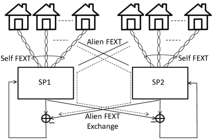
Figure 1: Interference Cooperation (IC) for multi-operator xDSL system.

Focus of this paper is the co-operation among SPs as envisioned in [11] to take the full advantage of vectoring in multi-operator settings. Cooperation among multiple SPs (Fig.1) being one alien-FEXT of the other is proposed here by avoiding the exchange of any sensitive data among SPs to guarantee that none of the other SPs can recover the information (either channel matrix and encoded data stream) of own users. The interference cooperation (IC) approach is based on the exchange of alien-FEXT only that is purposely removed as sketched in Fig.1. The iterative ICs that account either for multi-user channel estimation and multi-user detection are based on Expectation and Maximization (EM) estimation methods adapted to FEXT mitigation from cellular communications [12][13][14]. In this paper, these iterative EM methods are reformulated by guaranteeing that every SP exchanges the interference with others after stripping the information depending on the own users to have an IC that preserves the sensible information. Given the linearity of the communication model, multiple-channel estimation and multi-user detection are handled using the same principle, with slightly differences due to the peculiarities of the two processing steps. Even if the signaling of the inter-operator interference seems to be a trivial extension of EM methods, the specificities of interference cooperation need to address the overall multi-user channel estimation (comprehensive of alien-FEXT) and detection as a new problem.

Benefits from cooperation in multiple receiver systems was established based on information theoretic capacity of multi-receiver cellular network [15, 16], showing that the capacity loss due to inter-cell interference (i.e., alien-FEXT in wired systems) could be eliminated by cooperating base stations (BSs). In view to densify the BSs, multiple remote radio equipment are connected to a central BS through high speed link to get the benefit of central processing for up-link inter-cell interference mitigation [17]. Interference alignment and cancellation has been proposed and validated in field trials [18] but still based on exchange of encoded data. Interference cancellation based on iterative subtraction of interfering signals in cooperative BS clusters is in [19, 20]. Distributed BS co-operation scheme based on soft-combining for multi-user multi-cell system is in [21]. In all these schemes, the degree of co-operation is controlled by limiting the backhaul capacity. Mixed soft and hard information exchange among multiple BSs for interference cancellation is in [22]. All these methods, in addition to [23, 24, 25],[26], are excellent references to highlight the active research in the field of interference cancellation when multiple processing units need to cooperate by exchanging decoded (still sensitive) data to increase the spectrum efficiency in wireless and wired systems. However, this paper moves on a different conceptual setting where the exchanging among SPs is only the interference from received signals after iteratively stripping own sensitive data, or data mixed with an unknown mixing matrix acting as randomized multiplicative data perturbation [27].

Security and privacy are primary concerns in communication systems. Providing enough privacy should be also a challenge in any co-operative interference mitigation technique in multi-operator scenario due to the exchange of subscriber’s private information for the purpose of canceling the interference. Conventionally, security is provided at network layer for the well-known security threats e.g. eavesdropping, man-in-the-middle attack etc. [28, 29], but the concept of security is changing in the advanced communication system design. Examples of attacks on femtocells are in [30]. Recently, research community is giving more attention to physical layer security. Stochastic geometry approach for physical layer security in cellular system has been proposed in [31]. This paper is motivated by the need to do all necessary to prevent the other SPs to decode the information on own users still having a benefit from the mutual SPs cooperation.

I-A Contribution

Interference cooperation (IC) for multi-operator is the same for cellular and wired system, but in this paper we specialize the method for xDSL system, even if extension to multi-cell processing is conceptually straightforward with minor adaptations (not covered here). To better highlight the contribution, let us consider Fig.1 for the simple case of two SPs with one user each labeled as 1 and 2 (channel estimation would be similar except for larger size systems, see Section III). Signal model is

$$y_{1} = h_{11}x_{1}+h_{21}x_{2}+w_{1}\mathbf{=g}_{1}^{T}\mathbf{x}+w_{1}$$

$$y_{2} = h_{12}x_{1}+h_{22}x_{2}+w_{2}=\mathbf{g}_{2}^{T}\mathbf{x}+w_{2}$$

where SP 1 and 2 receive the interference from the other ($h_{21}x_{2}$ and $h_{12}x_{1}$), and $w_{1},w_{2}$ denote the additive white Gaussian noise (AWGN). In conventional data-exchange methods each SP is aware (or estimated separately) of the channel vector ${\bf g}_{1}=\left[h_{11},h_{21}\right]^{T}$ and ${\bf g}_{2}=\left[h_{12},h_{22}\right]^{T}$, symbols $x_{1}$ and $x_{2}$ are locally decoded as $\hat{x}_{1}$ and $\hat{x}_{2}$ (by SP 1 and 2, respectively) and iteratively exchanged to remove the crosstalk as $y_{1}-h_{21}\hat{x}_{2}$ to estimate $x_{1}$ by SP1, and similarly for SP2 with $y_{2}-h_{12}\hat{x}_{1}$.

In the proposed IC method, the overall system is modeled as:

$$\mathbf{y}=\left[\begin{array}[]{c}y_{1}\\ y_{2}\end{array}\right]=\mathbf{h}_{1}x_{1}+\mathbf{h}_{2}x_{2}+\mathbf{w}$$

with $\mathbf{h}_{1}=[h_{11},h_{12}]^{T}$ and $\mathbf{h}_{2}=[h_{21},h_{22}]^{T}$ the channels known to SP1 and SP2, respectively. The interference is exchanged at every iteration (i.e., based on the decoded $\hat{x}_{1}$, the residual $y_{1}-h_{11}\hat{x}_{1}$ and $h_{12}\hat{x}_{1}$are sent $1\rightarrow 2$ that use by SP2 for decoding ${\hat{x}_{2}}$; a similar reasoning holds true for signaling $2\rightarrow 1$) to yield the $2\times 1$ set of observations $\mathbf{y}-\mathbf{h}_{2}\hat{x}_{2}$ and $\mathbf{y}-\mathbf{h}_{1}\hat{x}_{1}$ at SP 1 and 2 to decode $\hat{x}_{1}$ and $\hat{x}_{2}$ using the locally known channels $\mathbf{h}_{1}$ and $\mathbf{h}_{2}$. Differently from conventional iterative receivers where each exchange of data is to guarantee that the other processing units can reduce the interference, here each interference exchange favors the other SPs. Even if interference exchange seems less efficient than encoded data exchange, this paper proves that the iterative method solves implicitly the centralized problem of data detection (and similarly for channel estimation) by reorganizing the interference exchange to carry out Jacobi iterations distributed over SPs, that in turn converge to the centralized interference cancellation method within few iterations at price of signaling overhead. The convergence-rate of IC depends on the degree of interference that is faster when the channel matrix is diagonal dominant, but still within 3-5iterations. Even if the exchange among SPs is interference-based to preserve the privacy on own users, there could be a way for the other SPs to infer the information on the own users (e.g., SP1 can extract $h_{21}\hat{x}_{2}$ after the stripping of SP2, but still mixed with unknown $h_{21}$ and $\hat{x}_{2}$) by using blind separation methods [32, 33]. However, blind-estimation methods need strict assumptions (e.g., known constellations and/or well algebraic structure of the channel) that make them unfeasible in practical xDSL systems (see Section III).

Paper is organized as follows. Section II illustrates the system model for multi-operator scenarios with self-FEXT and alien-FEXT. Section III describes the co-operative channel estimation using iterative information shared among the SPs that implements the EM method distributed among different SPs with partial information on the interference. Section IV describes the cooperative multi-user detection (MUD) still using iterative EM with MMSE estimator for multiple-operators. Numerical validations are in Section V, while Section VI draws some conclusions.

II System Model for Multi-operator Receiver

System model is for K-operators scenario with the channel matrices (or channels in short) for self- and alien-FEXT.

II-A Multi-operator System Model

Multi-operator xDSL system for upstream is shown in Fig.2, where multiple service providers (SPs) sharing the same cable binder have $N$ customer premises equipments (CPEs) labeled as $\text{CP}\text{E}_{1,i},\text{CP}\text{E}_{2,i},\ldots,\text{CP}\text{E}_{N,i}$ that are mutually interfering one another. To have an analytically tractable problem, here we assume that all the $K$ SPs have the same number of CPEs mutually synchronized with the same upstream frame structure without any frequency drift one another so that any inter-carrier interference can be neglected, and we can employ a system model that accounts for FEXT on each carrier independently.

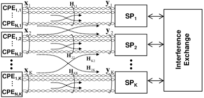
Figure 2: System model for cooperative xDSL with $K$ SPs and $N$ CPEs each

Fig.2 shows the ensemble of all $KN\times 1$ received signals $\mathbf{y}\left(t\right)$ at time $t$ as given by

$$\underset{\mathbf{y}\left(t\right)}{\underbrace{\left[\begin{array}[]{c}\mathbf{y}_{1}\left(t\right)\\ \mathbf{y}_{2}\left(t\right)\\ \vdots\\ \mathbf{y}_{\mathrm{K}}\left(t\right)\end{array}\right]}}=\underset{\mathbf{H}}{\underbrace{\left[\begin{array}[]{cccc}\mathbf{H}_{11}&\mathbf{H}_{21}&\ldots&\mathbf{H}_{\mathrm{K}1}\\ \mathbf{H}_{12}&\mathbf{H}_{22}&\ldots&\mathbf{H}_{\mathrm{K}2}\\ \vdots&\vdots&\ddots&\vdots\\ \mathbf{H}_{1\mathrm{K}}&\mathbf{H}_{2\mathrm{K}}&\ldots&\mathbf{H}_{\mathrm{K}\mathrm{K}}\end{array}\right]}}\underset{\mathbf{x}\left(t\right)}{\underbrace{\left[\begin{array}[]{c}\mathbf{x}_{1}\left(t\right)\\ \mathbf{x}_{2}\left(t\right)\\ \vdots\\ \mathbf{x}_{\mathrm{K}}\left(t\right)\end{array}\right]}}+\underset{\mathbf{w}\left(t\right)}{\underbrace{\left[\begin{array}[]{c}\mathbf{w}_{1}\left(t\right)\\ \mathbf{w}_{2}\left(t\right)\\ \vdots\\ \mathbf{w}_{\mathrm{K}}\left(t\right)\end{array}\right]}}$$ (1)

where $\mathbf{x}_{k}\left(t\right)=\left[x_{k,1}\left(t\right),x_{k,2}\left(t\right)\ldots,x_{k,N}\left(t\right)\right]^{T}$ denotes the signals from the finite alphabet $\Lambda$ of M-QAM constellation that is transmitted from the $N$ CPEs belonging to the $k$th SP. The ensemble of $NK\times 1$ transmitted signals related to all CPEs from all the $K$ SPs are in $\mathbf{x}\left(t\right)$. Each $N\times N$ matrix $\mathbf{H}_{ij}$ is the $i\rightarrow j$ channel from $N$ CPEs of the $i$th SP ($\text{CP}\text{E}_{1,i},\ldots,\text{CP}\text{E}_{N,i}$) towards the $j$th SP ($i\rightarrow j$) and it accounts for the channel including the self-FEXT (when $i=j$) and alien-FEXT (when $i\neq j$). $\mathbf{H}$ is the $KN\times KN$ channel matrix of the multi-user/multi-operator system. The AWGN ${\bf w}_{k}(t)$ is uncorrelated among CPEs and SPs, with the same power: $\mathbf{w}\left(t\right)\sim CN(0,\sigma^{2}\mathbf{I})$. Since the proposed IC method handles mutual interference as useful signals for the other SPs, for the scope of the paper the model (1) needs to be re-ordered by grouping the CPEs that belong to the same SP

$$\mathbf{y}\left(t\right)=\mathbf{H}_{1}\mathbf{x}_{1}\left(t\right)+\mathbf{H}_{2}\mathbf{x}_{2}\left(t\right)+\ldots+\mathbf{H}_{\mathrm{K}}\mathbf{x}_{\mathrm{K}}\left(t\right)+\mathbf{w}\left(t\right)$$ (2)

where ${\bf H}_{k}=\left[{\bf H}_{k1}^{T},{\bf H}_{k2}^{T},\ldots,{\bf H}_{kK}^{T}\right]^{T}$ is the compound channel from the $N$ CPEs belonging to the $k$th SP ($\text{CP}\text{E}_{1,k},\ldots,\text{CP}\text{E}_{N,k}$) toward all the SPs as sketched in Fig.2. The arrangement (2) will be used by the $k$th SP to estimate the $KN\times N$ channel ${\bf H}_{k}$ in IC channel estimation (Section III), or in detection assuming ${\bf H}_{k}$ is known (Section IV). Model for interference co-operation among the $K$ SPs is shown in Fig.2, where all SPs share alien-FEXT interference information by using backhaul for interference exchange that let every SP forward to all the $K-1$ SPs the received alien-interference after stripping the own data. For $K=2$ it reduces to a single-link between SP1 and SP2.

To separate channel estimation from decoding beyond the logical separation, the transmission is organized into frames with a frame structure that alternates a set of training samples with data to be decoded. The $k$th SP assigns to its $N$ CPEs $T$ samples of the training sequences $\left\{\overline{\mathbf{x}}_{k}\left(t\right)\right\}_{t=1}^{T}$ selected independently by the $k$th SP. Training used by the $k$th SP are not known to the other SPs to prevent estimation of alien-FEXT by other SPs. To ease the attention on IC method, training can be considered as ideal (i.e., mutually orthogonal) even if some degradation is expected when this condition is not met. Needless to say that the channel estimation step includes the estimate of any frequency drift and their correction for the own CPEs, if necessary (not covered here). Channel estimation and MUD are discussed below as two distinct processing steps, still sharing several commonalities due to the linear model (2).

II-B Self and Alien channel models

Channel model depends on the cable length and frequency range as increasing the frequency strengthen the inter-cable coupling, and this makes the FEXT comparable with losses of direct links (insertion loss). A simple model adopted here for numerical validations is based on the assumption that the direct links are normalized to have unit-amplitude, and the degree of diagonal dominance for self-FEXT channel $\mathbf{H}_{ii}$ and alien-FEXT channel $\mathbf{H}_{ij}$ (from $\{\text{CP}\text{E}_{\ell,i}\text{\}}_{\ell=1}^{N}$ to $\mathit{j}$th SP) is accounted in terms of scaling term $\alpha$, the entries are

$${\bf H}_{ii}[p,p]=e^{j\theta_{p}}\text{ with }\theta_{p}\sim{\mathcal{U}}(0,2\pi)$$ (3)

$${\bf H}_{ij}[p,q]\sim\mathcal{C}\mathcal{N}(0,\alpha^{2}),\forall p\neq q$$ (4)

with the same coupling $\alpha$ for both self- and alien-FEXT.

Off-diagonal terms are as small as $\alpha<-10dB$ up to 10-30MHz bandwidth [34] [14], these values are compliant with channel measurements of 24 pairs (0.5mm/ea) over 200m twisted pair cable up to 80-100MHz bandwidth as for next generation DSL [35]. The FEXT coupling $\alpha$ increases vs frequency and for long-cables, it is not so unusual to have a FEXT that is comparable to direct link when above 50-100MHz as for G.fast settings [5] adopted in numerical validations (Section V).

III Cooperative Channel Estimation

The training sequences are composed of a set of $T$ complex-valued samples ($T>N$) transmitted by all the $KN$ CPEs at the same time. The $N\times T$ training sequence matrix for the $N$ CPEs of $k$th SP {$\text{CP}\text{E}_{\ell,k}\text{\}}_{\ell=1}^{N}$ is

$$\overline{\mathbf{X}}_{k}=\left[\overline{\mathbf{x}}_{k}\left(1\right),\overline{\mathbf{x}}_{k}\left(2\right),\ldots,\overline{\mathbf{x}}_{k}\left(T\right)\right],$$ (5)

over-bar denotes the frame of training sequences. These training are pseudo-random sequences assigned by SP to every CPE and never exchanged among the SPs so the $k$th SP knows $\overline{\mathbf{X}}_{k}$, but not the others. To simplify, it is assumed that the training sequences of one SP are mutually uncorrelated with training sequences of other $K-1$ SPs and have ideal auto-correlation so that $\overline{\mathbf{X}}_{k}\overline{\mathbf{X}}_{k}^{H}=\mathbf{I}$ and $\overline{\mathbf{X}}_{k}\overline{\mathbf{X}}_{i}^{H}=\mathbf{0}$ for all $i\neq k$. Notice that for random selection of the training sequence as in practice happens, these ideal properties hold only approximately at price of a negligible loss of performance (Section V). The discrete signal received at $k$th SP ${\bf Y}_{k}=[{\bf y}_{k}(1),{\bf y}_{k}(2),\ldots,{\bf y}_{k}(T)]$ is

$$\mathbf{Y}_{k}=\mathbf{H}_{kk}\overline{\mathbf{X}}_{k}+\sum\limits_{m\neq k}\mathbf{H}_{mk}\overline{\mathbf{X}}_{m}+\mathbf{W}_{k}$$ (6)

here separated into own data ($\mathbf{H}_{kk}\overline{\mathbf{X}}_{k}$) and alien-FEXT ($\sum\limits_{m\neq k}\mathbf{H}_{mk}\overline{\mathbf{X}}_{m}$). Below the conventional Data Cooperation (DC) is discussed first as reference scenario, and then the method based on Interference Cooperation (IC).

III-A Data Cooperation (DC)

In DC the initial signaling setup lets all SPs be aware of the training sequence of all the other SPs. In this case the channel estimation can be carried out by each SP to attain the centralized approach where virtually one SP collects all the received signals. More specifically, when the $k$th SP is aware of all training $\overline{\mathbf{X}}=\left[\overline{\mathbf{X}}_{1}^{T},\overline{\mathbf{X}}_{2}^{T},\ldots,\overline{\mathbf{X}}_{K}^{T}\right]^{T}$, the model (6) becomes:

$$\mathbf{Y}_{k}=\mathbf{G}_{k}^{T}\overline{\mathbf{X}}+\mathbf{W}_{k}$$ (7)

where ${\bf G}_{k}^{T}=\left[{\bf H}_{1k},\cdots,{\bf H}_{kk},\ldots,{\bf H}_{Kk}\right]$ collects the channels from all $\text{CP}\text{E}_{\ell,i}$ toward $k$th SP. Maximum likelihood estimation (MLE) of this compound channel is

$$\widehat{\mathbf{G}}_{k}=\mathbf{Y}_{k}\overline{\mathbf{X}}^{H}(\overline{\mathbf{X}}\overline{\mathbf{X}}^{H})^{-1}$$ (8)

According to the properties of training sequence, the covariance of the channel estimate $\widehat{\mathbf{G}}_{k}$ is

$$\operatorname{cov}(\widehat{{\bf G}}_{k})\geq\frac{\sigma^{2}}{T}{\bf I},$$ (9)

that is the Cram r Rao bound of the channel estimate. These estimates are independent and error scales with the training sequence length $T$ and AWGN power $\sigma^{2}$. Once again, it is crucial to remark that DC mimics the centralized approach so that $k$th SP estimates self-FEXT (${\mathbf{H}_{kk}}$) and all the alien-FEXT (${\mathbf{H}_{mk}}$ for $\forall m\neq k$) channels that are locally used by $k$th SP in MUD. If channel is slowly varying as in wired system, this method needs a minimal inter-SP signaling at setup to have a consensus among the usage of training and the channel estimations can be carried out independently by each SP according to (8).

III-B Interference Cooperation (IC)

IC method is iterative and implies not to exchange the training among the SPs (as considered a sensitive information) but rather the training-induced FEXT. The model for channel estimation by the $k$th SP as the SP of interest is by collecting the $T$ training samples into $\mathbf{Y}=\left[\mathbf{y}(1),\mathbf{y}(2),\ldots,\mathbf{y}(T)\right]$ according to (2):

$$\mathbf{Y}=\mathbf{H}_{k}\overline{\mathbf{X}}_{k}+\sum\limits_{m\neq k}\mathbf{H}_{m}\overline{\mathbf{X}}_{m}+\mathbf{W\mathrm{,}}$$ (10)

where contribution by the different CPEs are grouped according to their SPs. Since each SP is only aware of its own training sequence, after the $k$th SP receives the alien-FEXT signaling from all the other $K-1$ SPs in the form of $\mathbf{Y}_{m}-\sum\limits_{l\neq k}\mathbf{H}_{lm}\overline{\mathbf{X}}_{l}$ (say from the $m$th SP with$m\neq k$), it stacks all the received alien-FEXT to locally reproduce the following model complementary to (10)

$$\mathbf{Y}-\sum\limits_{m\neq k}\mathbf{H}_{m}\overline{\mathbf{X}}_{m}=\mathbf{H}_{k}\overline{\mathbf{X}}_{k}+\mathbf{W\mathrm{,}}$$ (11)

after the signals from all interfering SPs are stripped out from each SP and forwarded to the $k$th one. The linear model (11) is solved iteratively in the IC method as detailed below.

Let $\mathbf{H}_{kk}^{(1)}$ be the initial estimate at $k$th SP by assuming that alien-FEXT is an augmented AWGN, the $k$th SP exchanges $\mathbf{Y}_{k}-\mathbf{H}_{kk}^{(1)}\overline{\mathbf{X}}_{k}$ with the other $K-1$ SPs in trade of $\mathbf{Y}_{m}-\mathbf{H}_{mm}^{(1)}\overline{\mathbf{X}}_{m}$ one by one from all the others SPs (here $m\neq k$ denotes any arbitrary SP different from the $k$th one). At the $n$th iteration of the iterative IC method, the $k$th SP estimates $\mathbf{H}_{km}^{(n)}$ and this is re-encoded as $\mathbf{H}_{km}^{\left(n\right)}\overline{\mathbf{X}}_{k}$ and forwarded to the $m$th SP in form of alien-FEXT, and similarly each of the other $K-1$ SPs re-encodes $\mathbf{H}_{mk}^{\left(n\right)}\overline{\mathbf{X}}_{m}$ for the benefit of $k$th SP. The interference is thus exchanged among all the $K$ SPs one by one as $N\times T$ matrices. $k$th SP uses the received re-encoded interference for alien-FEXT cancellation and iterative channel estimation based on the linear model (11) adapted for the iterations. It must be noticed that at every iteration the estimate by the $k$th SP is the channel $KN\times N$ matrix $\mathbf{H}_{k}=\left[\mathbf{H}_{k1}^{T},\mathbf{H}_{k2}^{T},\ldots,\mathbf{H}_{kK}^{T}\right]^{T}$ that stacks not only self-FEXT ($\mathbf{H}_{kk}^{(n)}$), but also alien-FEXT channels from own CPEs towards the other SPs ($\mathbf{H}_{km}^{(n)}$ for $m\neq k$). At every iteration, the cost function is

$$\mathbf{H}_{k}^{\left(n+1\right)}=\arg\mathop{\min}\limits_{{\mathbf{H}_{k}}}\left\|\mathbf{Z}_{k}^{(n)}-\mathbf{H}_{k}\overline{\mathbf{X}}_{k}\right\|^{2}$$ (12)

where $\mathbf{Z}_{k}^{(n)}=\mathbf{Y}-\sum\limits_{m\neq k}\mathbf{H}_{m}^{\left(n\right)}\overline{\mathbf{X}}_{m}$ is the effective variable that collects all interference $\mathbf{H}_{m}^{\left(n\right)}\overline{\mathbf{X}}_{m}$ exchanged by the $K-1$ SPs ($m\neq k$) locally used for refinement of $\mathbf{H}_{k}$. The estimation of $\mathbf{H}_{k}$ becomes

$$\mathbf{H}_{k}^{\left(n+1\right)}=\mathbf{Z}_{k}^{(n)}\overline{\mathbf{X}}_{k}^{H}(\overline{\mathbf{X}}_{k}\overline{\mathbf{X}}_{k}^{H})^{-1}$$ (13)

Once again, SPs cooperation refines self-FEXT and alien-FEXT by constraining the cooperation among SPs to never exchange the training $\overline{\mathbf{X}}_{k}$ and $\overline{\mathbf{X}}_{m}$ among each other, at most mixed by the (unknown) channel responses. The iterative channel estimation algorithm is summarized in Algorithm-1 for the $k$th SP.

Algorithm 1 Upstream Multi-operator Interference Cooperation Channel Estimation

• Initialize ${\bf{H}}_{kk}^{\left(1\right)}={{\bf{Y}}_{k}}\overline{{\bf{X}}}_{k}^{H}{(\overline{{\bf{X}}}_{k}\overline{{\bf{X}}}_{k}^{H})^{-1}}$

• Receive alien-FEXT ${{\bf{Y}}_{m}}-{\bf{H}}_{mm}^{\left(1\right)}{\overline{{\bf{X}}}_{m}}$ from all $K-1$ SPs ($m\neq k$).

• Interference exchange ($m\leftrightarrow k$): evaluate ${\bf{H}}_{km}^{\left({1}\right)}=({{\bf{Y}}_{m}}-{\bf{H}}_{mm}^{\left({1}\right)}{\overline{{\bf{X}}}_{m}})\overline{{\bf{X}}}_{k}^{H}{(\overline{{\bf{X}}}_{k}\overline{{\bf{X}}}_{k}^{H})^{-1}}$ and forward ${\bf{H}}_{km}^{\left({1}\right)}{\overline{{\bf{X}}}_{k}}$ to $m$th SP in exchange of ${\bf{H}}_{mk}^{\left({1}\right)}{\overline{{\bf{X}}}_{m}}$.

• for $n=1:{N_{iteration}}$

  • Estimate

    $${\bf{H}}_{kk}^{\left({n+1}\right)}=\left({{{\bf{Y}}_{k}}-\sum\limits_{m\neq k}{{\bf{H}}_{mk}^{(n)}{{\overline{{\bf{X}}}}_{m}}}}\right)\overline{{\bf{X}}}_{k}^{H}{({\overline{{\bf{X}}}_{k}}\overline{{\bf{X}}}_{k}^{H})^{-1}}$$

  • Receive alien-FEXT ${{\bf{Y}}_{m}}-{\bf{H}}_{mm}^{\left({n+1}\right)}{\overline{{\bf{X}}}_{m}}-\sum\limits_{p\neq m,k}{{\bf{H}}_{pm}^{\left(n\right)}{{\overline{{\bf{X}}}}_{p}}}$ from all $K-1$ SPs ($m\neq k$).

  • Interference exchange ($m\leftrightarrow k$): evaluate ${\bf{H}}_{km}^{\left({n+1}\right)}=({{\bf{Y}}_{m}}-{\bf{H}}_{mm}^{\left({n+1}\right)}{\overline{{\bf{X}}}_{m}}-\sum\limits_{p\neq m,k}{{\bf{H}}_{pm}^{\left(n\right)}{{\overline{{\bf{X}}}}_{p}}})\overline{{\bf{X}}}_{k}^{H}{({\overline{{\bf{X}}}_{k}}\overline{{\bf{X}}}_{k}^{H})^{-1}}$ and forward ${\bf{H}}_{km}^{\left({n+1}\right)}{\overline{{\bf{X}}}_{k}}$ to $m$th SP in exchange of ${\bf{H}}_{mk}^{\left({n+1}\right)}{\overline{{\bf{X}}}_{m}}$.

III-B1 Convergence of IC

Iterative IC method for channel estimation is equivalent to iteratively solve the linear system of equations for the (centralized) model $\mathbf{Y}=\mathbf{H}\overline{\mathbf{X}}+\mathbf{W}$ from the (1). In other word, given the centralized model $\mathbf{Y}=\mathbf{H}\overline{\mathbf{X}}+\mathbf{W}$, the training can be partitioned into self and alien-FEXT training ($\overline{\mathbf{X}}=\overline{\mathbf{X}}_{s}+\overline{\mathbf{X}}_{a}$) so that the IC can be rewritten as ${\bf Y}={\bf H}^{(n+1)}\overline{{\bf X}}_{s}+{\bf H}^{(n)}\overline{{\bf X}}_{a}+{\bf W}$, this is the basis to prove that the iterations in IC is equivalent to Jacobi iteration [36] for channel estimation such that the estimate is carried out independently by each SP without exchanging $\overline{\mathbf{X}}_{a}$ but rather in form of mixed values ${\bf H}^{(n)}\overline{{\bf X}}_{a}$. Some technicalities are necessary for the equivalence. Let $\mathbf{M}=blockdiag\left[\mathcal{X}_{1},\mathcal{X}_{2},\ldots,\mathcal{X}_{K}\right]$ be the block diagonal of the training sequences known by each SP, where $\mathcal{X}_{k}=\mathbf{I}_{K}\otimes\overline{\mathbf{X}}_{k}^{T}\otimes\mathbf{I}_{N}$ here reordered just to comply with matrix algebra computations, the block off-diagonal term $\mathbf{N}=\mathbf{M}-\left(\mathbf{1}_{K}\otimes\left[\mathcal{X}_{1},\mathcal{X}_{2},\ldots,\mathcal{X}_{K}\right]\right)$ denotes the matrix with training for alien-FEXT, the IC method (Algorithm 1) reduces to the set of Jacobi iterations

$$\mathbf{M}\cdot vec\left(\mathbf{H}^{(n+1)}\right)=\mathbf{N\cdot}vec\left(\mathbf{H}^{(n)}\right)+\left(\mathbf{1}_{K}\otimes vec(\mathbf{Y})\right)$$ (14)

distributed over the SPs as each SP iteration refines (locally) a portion of the channel estimate $vec\left(\mathbf{H}^{(n)}\right)$ where the estimates by each SP are arranged into a vector by $vec(.)$ operator. Proof of convergence of Jacobi iterations is in Appendix-A, but since Jacobi iteration converge to $\mathbf{H}^{(n)}=\mathbf{Y}\overline{\mathbf{X}}^{H}(\overline{\mathbf{X}}\overline{\mathbf{X}}^{H})^{-1}$ for $n$ large enough (in practice, after 3-5 iterations, see Section V) the IC converge to the centralized MLE of the channel matrix without any exchange of data/training except as mixed values. It is crucial to remark again that in IC method the channels ${\bf H}_{k}=\left[{\bf H}_{k1}^{T},{\bf H}_{k2}^{T},\ldots,{\bf H}_{kK}^{T}\right]^{T}$ that cause alien-FEXT towards the other remaining $K-1$ SPs is the one that is updated within the $k$th SP. At convergence, this information is resident in $k$th SP in form of channel estimates, and this enables the IC Multi-user Detection (IC-MUD) as detailed below.

IV Cooperative Multi-user Detection

Data detection in multi-operator environment is based on channel state information available at each SP and the degree of cooperation among SPs. To ease the analysis still consistent with the problem at hand, the channels are assumed as random and mutually orthogonal i.e. $E\left[\mathbf{H}_{ii}^{H}\mathbf{H}_{ij}\right]=0,\forall i\neq j$. The signals received at $k$th SP for data detection follows from (1) (time index $t$ is omitted to simplify the notation):

$$\mathbf{y}_{k}=\mathbf{H}_{kk}\mathbf{x}_{k}+\sum\limits_{m\neq k}\mathbf{H}_{mk}\mathbf{x}_{m}+\mathbf{w}_{k}$$ (15)

where $\mathbf{H}_{kk}\mathbf{x}_{k}$, $\mathbf{H}_{mk}\mathbf{x}_{m}$ and $\mathbf{w}_{k}$ accounts self-FEXT, alien-FEXT and AWGN. The iterative MUD for Data Cooperation (DC) and Interference Cooperation (IC) are based on the EM method [12, 13, 40, 41], and these iterative methods are compared to the centralized MUD (i.e., all the SPs are decoded jointly) used as a reference scenario.

Once defined the linear model, MUD can be based either on zero-forcing (ZF) or minimum mean square (MMSE) criteria depending on the diagonal dominance of the channel model [4]. Herein all MUD methods are based on the matrix decision-feedback equalizer (DFE) from QR decomposition of the corresponding channel (or equivalently, BLAST system) either using ZF or MMSE criteria as widely investigated and adopted in vectoring (see e.g., [42] and [4]). To simplify the notation of MUD, the metrics are referred to ZF-MUD and matrix DFE are left indicated as well established.

IV-A Centralized Multi-user Detection

In centralized MUD all SPs forward the received signals to a central processing unit that is aware of all channels $\mathbf{H}$ (possibly estimated) and jointly decodes all the data streams according to the system model (1). The ZF-MUD is

$$\widehat{\mathbf{x}}=\mathbf{H}^{-1}\mathbf{y},$$ (16)

and the variance of the noise at decision variable is lower bounded by $\sigma^{2}/(1+(NK-1)\alpha^{2})$, it decreases with the number of cooperating SPs ($K$) and CPEs ($N$) due to the augmentation of signal flows in vectoring. For larger bandwidth (say >50MHz) the FEXT-coupling increases and the MMSE-MUD with matrix-DFE takes more efficiently into account the higher FEXT in vectoring. Signaling constraints for data-rate and privacy issues make the full cooperation with centralized MUD unfeasible but still it is an excellent reference bound in performance analysis (Section V).

IV-B Data Cooperation (DC) MUD

In DC iterative technique, it is assumed that the channel $\mathbf{G}_{k}^{T}=\left[\mathbf{H}_{1k},\ldots,\mathbf{H}_{kk},\ldots,\mathbf{H}_{Kk}\right]$ is known to $k$th SP, or estimated as a separated step discussed in Section III-A. At every iteration (say $n$th), every SP forwards its decoded data $\mathbf{x}_{m}^{(n)}$ to all the other $K-1$ SPs that in turn cancel locally the alien-FEXT using all the received data from the $K-1$ SPs after channel reshaping $\mathbf{H}_{mk}\mathbf{x}_{m}^{\left(n\right)}$, this step employs the following model for every iteration

$$\mathbf{y}_{k}-\sum\limits_{m\neq k}\mathbf{H}_{mk}\mathbf{x}_{m}^{(n)}=\mathbf{H}_{kk}\mathbf{x}_{k}+\mathbf{w}_{k}$$ (17)

The ZF-MUD simplifies into a set of soft-detection for each decision variable as [12]:

$$\mathbf{x}_{k}^{(n)}=g_{\Lambda}\left[\frac{\mathbf{H}_{kk}^{-1}}{\sigma_{n}^{2}}\left(\mathbf{y}_{k}-\sum\limits_{m\neq k}\mathbf{H}_{mk}\mathbf{x}_{m}^{(n)}\right)\right]$$ (18)

where $g_{\Lambda}[x]=E_{x\in\Lambda}\{x|x+z\}$ is the symbol-based MMSE estimator at the decision variable and $\sigma_{n}^{2}$ is the corresponding (iteration varying) variance of the noise at the decision variable. The soft-decision $g_{\Lambda}[.]$ is modulation-dependent as described in Appendix C, and it reduces to $\tanh[.]$ for BPSK and QPSK modulations [12]. Smoothness depends on $1/\sigma_{n}^{2}$ and it can be “hardened” (by reducing $\sigma_{n}^{2}$) at last iterations, if necessary, or by updating its value as in [24]. The same soft-decisions are employed within the loop of the matrix-DFE to avoid error propagation within the same SP.

At 1st iteration, data from other SPs are not available at any SP, therefore from the received signal $\mathbf{y}_{k}$ the noise at decision variable is assumed Gaussian and alien-FEXT augments the AWGN: $\mathbf{H}_{kk}^{-1}(\sum\limits_{m\neq k}\mathbf{H}_{mk}\mathbf{x}_{m}+\mathbf{w}_{k})\sim CN\left(0,\sigma_{1}^{2}\mathbf{I}\right)$ with $\sigma_{1}^{2}=\left(\left(K-1\right)N\alpha^{2}+\sigma^{2}\right)/(1+(N-1)\alpha^{2})$. Once the decoded data is shared among the SPs, the variance at decision variable progressively reduces down to the (almost) complete alien-FEXT cancellation $\sigma_{n}^{2}=\sigma^{2}/(1+(N-1)\alpha^{2})$, for $n$ large enough. However, it must be noticed that the noise variance in DC is always higher than the centralized approach as in DC only the $N$ self-FEXT links are used for data estimation rather than in centralized vectoring approach where all $KN$ links contributes in decoding. Compared to centralized vectoring, the degradation of noise power at decision variable for DC is at least

$$\text{DC}_{loss}=1+\frac{N(K-1)\alpha^{2}}{1+(N-1)\alpha^{2}}$$ (19)

that for a very large number of CPEs it depends on $K$ as DC${}_{loss}\simeq K$.

IV-C Interference Cooperation (IC) MUD

For IC method, the reference system is (2) and the ensemble of channels ${\bf H}_{k}=\left[{\bf H}_{k1}^{T},{\bf H}_{k2}^{T},\ldots,{\bf H}_{kK}^{T}\right]^{T}$ is known to $k$th SP as being estimated by the IC channel estimation (Section III-B). At each iteration, all the $K$ SPs estimates the symbols $\mathbf{x}_{1}^{(n)},\mathbf{x}_{2}^{(n)},...,\mathbf{x}_{K}^{(n)}$ and forward each-others the received signals after stripping the own signals and leaving the alien-FEXT. Focusing to the $k$th SP, it stacks all the measurements received by all the K-1 SP into the $KN\times 1$ vector

$$\mathbf{z}_{k}^{(n)}=\mathbf{y}-\sum\limits_{m\neq k}\mathbf{H}_{m}\mathbf{x}_{m}^{\left(n\right)}$$ (20)

that is the results of stripping $\mathbf{x}_{m}^{(n)}$ with the local $KN\times N$ mixing channel$\mathbf{H}_{m}$ known only to the $m$th SP ($m\neq k$) as detailed in Section III. The model at the $k$th SP reduces to

$$\mathbf{z}_{k}^{(n)}=\mathbf{H}_{k}\mathbf{x}_{k}+\mathbf{w},$$ (21)

that is made redundant by $KN$ lines as the result of the augmentation from the alien-FEXT exchange.

Signaling exchange and MUD processing for (21) is detailed in Algorithm 2 for ZF criteria (MMSE differs only for the metric), and it is illustrated by focusing to a pair of SPs, say $m$th and $k$th. The $m$th SP estimate $\mathbf{x}_{m}^{(n)}$ is mixed with (locally available) channel $\mathbf{H}_{mk}$ to have $\mathbf{H}_{mk}\mathbf{x}_{m}^{(n)}$ that is forwarded to the $k$th SP, and symmetrically from $k$th SP so that the interference is exchanged one-by-one among all the $K$ SPs. Based on these exchanges, $k$th SP mitigates the alien-FEXT from the locally received signal $\mathbf{y}_{k}$ as $\mathbf{y}_{k}-\sum\limits_{m\neq k}\mathbf{H}_{mk}\mathbf{x}_{m}^{(n)}$. Similarly, the $m$th SP estimates the alien-FEXT contribution from $k$th SP as $\mathbf{y}_{m}-\sum\limits_{l\neq k}\mathbf{H}_{lm}\mathbf{x}_{l}^{(n)}$ using own CPEs ($\mathbf{H}_{mm}\mathbf{x}_{m}^{(n)}$) and alien-FEXT ($\mathbf{H}_{lm}\mathbf{x}_{l}^{(n)}$ for $l\neq k,m$) received from the other SPs. The estimated alien-FEXT is again exchanged among all the $K-1$ SPs and the $k$th SP to locally build the new $KN\times 1$ vector (20) for MUD ${\bf x}_{k}^{\left(n+1\right)}$.

After mutual alien-FEXT signaling, the estimation of $\mathbf{x}_{k}^{\left(n+1\right)}$ from the linear model (21) is carried as part of the EM iterations [12, 13]. Namely, the cost function for ZF-MUD (similarly for MMSE-MUD) is given by

$$\mathbf{x}_{k}^{\left(n+1\right)}=\arg\min\limits_{\mathbf{x}_{k}}\left\|\mathbf{z}_{k}^{(n)}-\mathbf{H}_{k}\mathbf{x}_{k}\right\|^{2}$$ (22)

and it is be solved by matrix-DFE from QR decomposition of the compound $KN\times N$ mixing channel$\mathbf{H}_{k}$ (see Algorithm 2 for details). Due to the iterative exchange of alien-FEXT in interference cancellation, it is convenient to adopt the soft-estimates to avoid error propagation and have a gain in SNR of approx. 5dB (Section V) in line with ref.[24]. The MUD of the symbols at $(n+1)$th iteration becomes:

$$\mathbf{x}_{k}^{\left(n+1\right)}=g_{\Lambda}\left[\frac{1}{\sigma_{n}^{2}}(\mathbf{H}_{k}^{H}\mathbf{H}_{k})\mathbf{H}_{k}^{H}\mathbf{z}_{k}^{(n)}\right]$$ (23)

where $\sigma_{n}^{2}$ is the variance of the noise at decision variable for IC method and $g_{\Lambda}[.]$ is symbol-based MMSE estimator based on the alphabet $\Lambda$ (Appendix C). Variance $\sigma_{n}^{2}$ reduces vs iterations and it can be calculated while evaluating the new soft-decisions [24].

At the setup, there is no information available on alien-FEXT and thus the estimate (23) is replaced by the estimate based on $\mathbf{y}_{k}$ that accounts for alien-FEXT as an augmented AWGN. After the 1st iteration, IC and DC differ as received signals are stripped of the own data to form the exchange signal $\mathbf{y}_{k}-\sum\limits_{m\neq k}\mathbf{H}_{mk}\mathbf{x}_{m}^{(n)}$ as detailed above (or in Algorithm 2). After alien-FEXT exchange, the noise power at decision variable is bounded by $\sigma^{2}/(1+(NK-1)\alpha^{2})$ as for centralized approach.

Algorithm 2 Upstream Multi-operator Cooperative ZF-MUD

• QR decomposition of $\mathbf{H}_{kk}$ (iteration 0): $\mathbf{Q\mathbf{R}}=\mathbf{H}_{kk}$, and ${\bf\widetilde{y}}_{k}=\mathbf{Q}^{H}{\bf y}_{k}$.

• Initialize

  $$\left[\mathbf{x}_{k}^{(1)}\right]_{i}=g_{\Lambda}\left[\frac{1}{\sigma_{n}^{2}}\left(\frac{1}{r_{i,i}}\left[{\bf\widetilde{y}}_{k}\right]_{i}-\sum\limits_{j=i+1}^{N}\frac{r_{i,j}}{r_{i,i}}\left[\mathbf{x}_{k}^{(1)}\right]_{j}\right)\right]$$

  , for $i=N,N-1,\ldots,1$

• QR decomposition of $\mathbf{H}_{k}$ (iteration $n\geq 1$):$\mathbf{Q\mathbf{R}}=\mathbf{H}_{k}$,

• for $n=1:N_{iteration}$

  • Receive ${\bf H}_{mk}{\bf x}_{m}^{\left(n\right)}$ from all$K-1$ SPs ($m\neq k$).

  • Interference exchange ($k\leftrightarrow m$): evaluate ${\bf y}_{k}-\sum\limits_{l\neq m}{\bf H}_{lk}{\bf x}_{l}^{\left(n\right)}$ and forward to $m$th SP in exchange of ${\bf y}_{m}-\sum\limits_{l\neq k}{\bf H}_{lm}{\bf x}_{l}^{\left(n\right)}$.

  • Estimate

    $$\left[\mathbf{x}_{k}^{(n+1)}\right]_{i}=$$

    $$g_{\Lambda}\left[\frac{1}{\sigma_{n}^{2}}\left(\frac{1}{r_{i,i}}\left[\tilde{\mathbf{z}}_{k}^{(n)}\right]_{i}-\sum\limits_{j=i+1}^{N}\frac{r_{i,j}}{r_{i,i}}\left[\mathbf{x}_{k}^{(n+1)}\right]_{j}\right)\right]$$

    , for $\tilde{\mathbf{z}}_{k}^{(n)}=\mathbf{Q}^{H}\mathbf{z}_{k}^{(n)}$

  • Update $\sigma_{n}^{2}$ based on ${\bf x}_{k}^{\left(n+1\right)}$

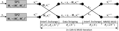
Figure 3: Signaling and Computational Complexity at each SP for $K=2$.

Fig.3 illustrates the $(n+1)$th iteration of IC MUD Algorithm 2 for $K=2$, there are two signaling phases with an overall signaling complexity $\mathcal{O}_{S}\left(2N\right),$ and computational complexity $\mathcal{O}_{C}\left(4N^{2}\right)$ at each SP. Generalization to arbitrary $K$ SPs makes the overall complexity $\mathcal{O}_{S}\left(2\left(K-1\right)N\right)$ and $\mathcal{O}_{C}\left(2KN^{2}\right)$. Compared to DC MUD with signaling complexity $\mathcal{O}_{S}\left(\left(K-1\right)N\right)$, the signaling of IC MUD is twice with remarkable benefits (Section V). Even if the data-rate is quite intensive, the SPs are hosted in the same cabinet on at short distance, and there are several parallelism that can be exploited in this setting for any practical implementations [43].

IV-C1 Convergence of ZF-MUD IC

Similarly to channel estimation (as IC MUD rely on the same linear model (1) used in multi-user channel estimation), the updating (23) is conceptually equivalent to the partition of the channel model into self ($\mathbf{H}_{s}$) and alien-FEXT ($\mathbf{H}_{a}$) so that the iterations reflect this partitioning eased by the IC signaling, and the local availability of channel matrices $\mathbf{H}_{k}$: $\mathbf{y}=\mathbf{H}_{s}\mathbf{x}^{(n+1)}+\mathbf{H}_{a}\mathbf{x}^{(n)}+\mathbf{w.}$ The proof of convergence toward the centralized estimate follows the same steps that highlights the equivalence between iterations (23) and the Jacobi method to solve the linear system $\mathbf{y}=\mathbf{Hx{\textstyle+}w}$ [36]. By reshaping the linear problem into block diagonal matrix $\mathbf{M}=blockdiag\left[\mathbf{H}_{1},\mathbf{H}_{2},\ldots,\mathbf{H}_{K}\right]$ that accounts for self-FEXT (say $\mathbf{H}_{s}$), and block off-diagonal matrix $\mathbf{N}=\mathbf{M}-\left(\mathbf{1}_{K}\otimes\left[\mathbf{H}_{1},\mathbf{H}_{2},\ldots,\mathbf{H}_{K}\right]\right)$ for alien-FEXT (say $\mathbf{H}_{a}$), each IC MUD is equivalent to the Jacobi iteration:

$$\mathbf{M}\mathbf{x}^{(n+1)}=\mathbf{N}\mathbf{x}^{(n)}+\left(\mathbf{1}_{K}\otimes\mathbf{y}\right)$$ (24)

carried out separately by each SP as MUD step (23), except for soft-detector $g_{\Lambda}[.]$ that is unavoidably related to the alphabet $\Lambda$ and used to prevent error propagation. Once again, the proof of convergence of Jacobi iterations (Appendix B) guarantees that IC converges to the same centralized vectoring solution for ZF metric. It can be shown that proof for MMSE-MUD IC follows the same steps.

IV-C2 Privacy

The exchange between any two SP is mixed by alien-FEXT channel that is never know according to the IC method for channel estimation (Section III). The $k$th SP could recover the mixed signal $\mathbf{H}_{mk}\mathbf{x}_{m}^{(n)}$ but this is without the knowledge of the mixing alien-FEXT channel $\mathbf{H}_{mk}$ that in IC method is not known to the $k$th SP, but only to the $m$th SP, and this randomizes $\mathbf{x}_{m}^{(n)}$ to preserve its the privacy [27]. Even if the exchange among SPs is interference-based, in principle there could be a way for the other SPs to infer the information on the own users. For the example at hand, the estimation of the alien information $\mathbf{x}_{m}^{(n)}$ could reduce to a multi-user blind separation from $\mathbf{H}_{mk}\mathbf{x}_{m}^{(n)}$ with the unknown mixing matrix $\mathbf{H}_{mk}$. However, even if the modulating terms are non-Gaussian as a necessary condition for blind-estimation methods, these are unknown in term of constellation, power (or scaling factor) and phase-stationarity (e.g., each user can have an arbitrarily rotated constellation specifically employed to prevent the decoding by alien SPs, but still being determistically known for the own SP) to prevent a reliable decoding of $N\times N$ MIMO mixing that, for the alien-FEXT channel $\mathbf{H}_{mk}$, it is likely below the decoding capability. In this sense the privacy can be considered pragmatically preserved to enable the adoption of IC methods from commercial operators and enable local loop unbundling.

V Numerical results

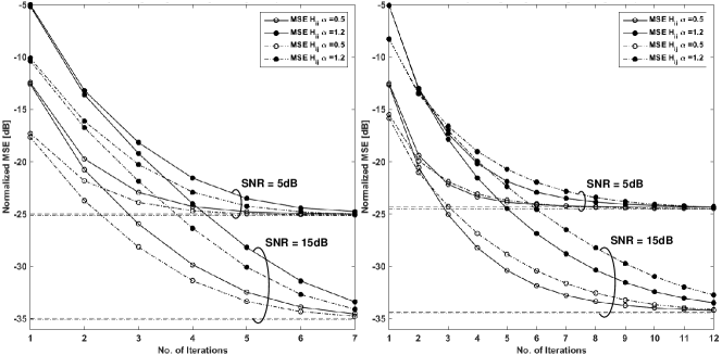
Figure 4: MSE vs Iterations($n$) of IC channel estimation in multi-operator xDSL for $SNR=[5,15]$dB,$\alpha=[0.5,1.2],K=2$ (left) and $K=3$ (right).

Numerical simulations validate the asymptotic performance of the IC method and evaluate the effectiveness of the cooperative method based on the exchange of interference only. We consider a scenario with $K=2$ and $3$ operators with $N=10$ CPEs each as being a reference for G.fast setting. Performances of the IC algorithms are evaluated either for statistical model [37] by varying the FEXT coupling $\alpha$, and by considering the cable-models of 100m length [35] up to the frequency of 200MHz to simulate the behavior in G.fast settings. In any case, the direct link is independent over the lines (all lines with the same length) so that $\mathbf{H}_{kk}[p,p]=\exp(j\theta_{p})$ with $\theta_{p}\sim\mathcal{U}(0,2\pi)$ statistically independent over lines. The transmitted symbols from every CPE belong to QAM constellation with a size that depends on the degree of G.fast specifications. Power spectral density of the signal at CPE is -76dBm/Hz and the noise is -140dBm/Hz as customary [35, 38, 39], signal to noise ratio (SNR) is always referred at the receiver unless defined at decision variable.

V-A Iterative Channel Estimation

Training are generated from a random set of QPSK symbols known to each SP as this approximates the ideal training with $\overline{\mathbf{X}}_{k}\overline{\mathbf{X}}_{k}^{H}\simeq\mathbf{I}$ and $\overline{\mathbf{X}}_{k}\overline{\mathbf{X}}_{i}^{H}\simeq\mathbf{0}$ for all $i\neq k$. Fig.4 shows MSE vs iterations of self ($\mathbf{H}_{ii}$) and alien-FEXT ($\mathbf{H}_{ij}$) channel estimates for $K=2$ and 3 operators scenario using IC, and the corresponding Cram r Rao Bound (CRB) (9). The performance has been evaluated for SNR$=1/\sigma^{2}\in\{5dB,15dB\}$ and FEXT coupling $\alpha\in\{0.5,1.2\}$ to validate the convergence of the proposed algorithms in these severe FEXT-conditions. The MSE is normalized by the power of channel for self-FEXT $\text{E}\left[\left\|\mathbf{H}_{ii}\right\|^{2}\right]$ and alien-FEXT $\text{E}\left[\left\|\mathbf{H}_{ij}\right\|^{2}\right]$; since $\text{E}\left[\left\|\mathbf{H}_{ii}\right\|^{2}\right]>\text{E}\left[\left\|\mathbf{H}_{ij}\right\|^{2}\right]$ the normalized MSE for $\mathbf{H}_{ii}$ is lower than MSE of $\mathbf{H}_{ij}$. Centralized method attains the CRB $MSE_{{\text{CRB}}}=trace\left[\sigma^{2}(\overline{\mathbf{X}}\overline{\mathbf{X}}^{H})^{-1}\right]$, and here IC attains the CRB in 3-5 iterations for $K=2$. When $K>2$ a larger number of iterations is necessary as the iterations are implicitly pairing the alien-FEXT to each users during the alien-FEXT exchange steps. If FEXT-coupling $\alpha$ is smaller, the number of iterations for IC convergence decreases as expected for smaller interference settings. In G.fast scenario the IC method converges (with in +2-3dB of excess MSE compared to CRB) in $2\div 3$ iterations up to a frequency of 100-120MHz, even if a practical convergence (not necessarily to the CRB) within 1-2 iterations. The cost of inter-SP signaling in this case is limited to the set-up phase and it needs not further optimizations to comply with inter-SP data-rate.

V-B Iterative Detection

Performance for multi-user/multi-operator detection are evaluated in term of SNR at decision variable ($SNR_{D}$) for different FEXT coupling and modulations. MMSE criteria for MUD is employed to cope with large FEXT coupling. Fig.5 shows the $SNR_{D}$ for varying $\alpha$ and SPs $K={2,3}$ for SNR $=1/\sigma^{2}=15dB$ scenario after 6-iterations for DC and IC methods with QPSK modulation. Performance of IC MMSE-MUD is compared with DC MMSE-MUD and MMSE-MUD with local vectoring (without alien-FEXT compensation) thus showing that the IC MMSE-MUD outperforms all the methods. Degradation with respect to centralized MUD is mainly due to error propagation for large FEXT coupling, soft-decoding in IC MUD prevents the propagation of errors and guarantees $SNR_{D}\geq 10dB$ even for $\alpha=0dB$ and $K=2,3$. Any inter-SP cooperation becomes mandatory for large degree of coupling, say $\alpha>-20$dB, with IC MUD uniformly when the error propagation dominates. Since in G.fast the crosstalk can be considered as $\alpha\geq-20dB$, the cooperation among SP should be considered as mandatory to make an efficient usage in any condition of coexistence of users within the same cable bundling.

h

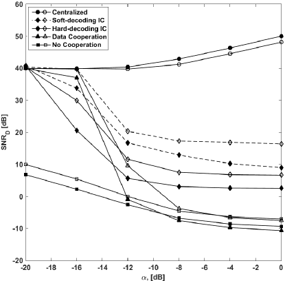
Figure 5: SNR at decision variable of MMSE-MUD methods vs $\alpha$ for $K=2$ (empty marker) and $K=3$ (filled marker) with $SNR=40dB$ and 6 iterations.

h

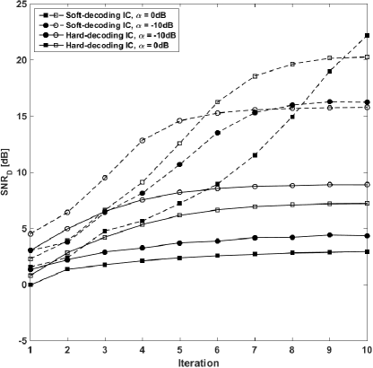
Figure 6: SNR at decision variable vs iterations of IC MMSE-MUD for $K=2$ (empty marker) and $K=3$ (filled marker), DFE with soft (dashed line) and hard (solid line) decisions, and varying $\alpha=${-10(circle),0(square)} dB. $(N=10,SNR=15dB)$

Convergence analysis of IC MMSE-MUD for QPSK with soft (empty-dots) and hard (filled dots) decisions DFE is in Fig.6 showing the $SNR_{D}$ vs iterations for $K=2,3$ and varying $\alpha$. Once again, this numerical results validates that the iterative IC algorithm converges into few iterations (say 3-5 iterations) for most practical purposes, with a remarkable benefit when using soft-decisions (23). Convergence is faster for smaller $\alpha$ and slower for large number of SPs (here K=3) as iterations implicitly ease the assignment to each SP the alien-FEXT corresponding to the own users to be exploited efficiently as “useful signal”.

Average performance from all lines vs frequency for G.fast channel model [35, 37] (cable length is 100m for all the CPEs, N=10 CPEs per SP and K=2 SPs) is in Fig.7, channel model is sketched on top-corner for insertion-loss (IL) and FEXT, and the corresponding $\alpha$. The thresholds on $SNR_{D}$ to attain the symbol error rate of $10^{-7}$ are superimposed for different QAM constellations, from BPSK to 4096-QAM. The MMSE-MUD for centralized system is the upper-bound with some dispersion of values (shaded area) but still above the BPSK threshold. The lack of any alien-FEXT mitigation as for no-cooperation scenario offers the lower bound. The DC MMSE-MUD method shows comparable performance with centralized MUD up to approx.120MHz (or equivalently from the channel parameters $\alpha<-10dB$) in accordance with threshold effect in Fig.5. IC MMSE-MUD (4 iterations) with soft-decoding outperforms the DC MUD and the same IC MUD with hard decoding for QPSK and 16-QAM (other modulations are consistent with these results), thus confirming all the results in Fig.5. In addition, the IC method guarantees the transport over all the G.fast bandwidth up to 212MHz.

h

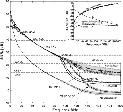
Figure 7: SNR at decision variable vs frequency in G.fast settings (cable length is 100m for all the CPEs, N=10 CPEs per SP and K=2 SPs) for MMSE-MUD: IC method with soft (SD) and hard (HD) decoding, centralized MUD, DC method. Channel losses are in top-right corner.

The SNR lets to compute the average throughput (Table 1) according to the “gap-formula” for bit-loading usually adopted in DSL [38, 39] for $SNR_{D}$ at $\ell$th tone

$$b_{\ell}=log_{2}\left(1+\frac{SNR_{D,\ell}}{\Gamma}\right)$$

where the gap $\varGamma$=10.8dB=6dB(SNR margin)+9.8dB(SNR gap)-5dB(coding gain) according to the ITU specifications for symbol error probability $10^{-7}$, maximum loading of 12bits and framing overhead is 12% [38]. Over the bandwidth 2-106MHz DC and IC attain the same throughput of centralized MUD, but when extending the bandwidth up to 212MHz the loss of IC MUD is negligible compared to centralized method, and the DC looses approx. 100MHz in throughput. The same Table shows that is it remarkably better to partition the overall bandwidth among the 2 SPs (e.g., alternate usage of the tones per SP) rather than allocate all the CPEs over the same bandwidth without any degree of cooperation, in this case the throughput is half the value for centralized (or IC) MUD.

Table I: Average throughput of different cooperation schemes for G. Fast settings (N=10, K=2, cable:100m)

Cooperation Scheme	2-106 MHz	2-212 MHz
Centralized	718 Mbps	884 Mbps
Equally shared bandwidth	357 Mbps	425 Mbps
Interference Cooperation (IC)	714 Mbps	854 Mbps
Data Cooperation (DC)	711 Mbps	756 Mbps
No Cooperation (NC)	275 Mbps	275 Mbps

VI Conclusions

Conventional interference mitigation techniques are based on centralized iterative interference cancellation that exchange data without any limitation on ownership. In this paper, we propose multi-user receivers employing channel estimation and detection in the multi-operator xDSL unbundling scenario where cooperation among different operators is obtained by exchanging the alien-interference considered as useful signal by the other operators. The IC method is iterative as interference exchange refines alien-interference and own data, and it has the merit that this cooperation among different service providers never exchange the decoded symbols considered as sensitive-information. Since each operator receives the interference from the others in exchange of their own, it can be considered an interference-based cooperation that can exploit all the redundancy from all the data-paths with respect to the other operators and thus the performance attains the same performance as a centralized vectoring method.

The convergence of IC is impaired by error propagation and soft-decision multi-user detection guarantees the convergence in few iterations (type.3-5 iterations) with a threshold in loss when overall interference becomes comparable with signal of interest. Even if data-rate exchange among operators is double the interference mitigation method by data exchange, the parallelism over frequency can be easily exploited in inter-operator communication using specific architectures [43].

Appendix A IC Channel Estimation Convergence

The exchanging of the interference reduces the channel estimation for $K$ SPs to the linear system (except AWGN that is irrelevant for MLE method) $\mathbf{Y}=\mathbf{H}\overline{\mathbf{X}}$, after vectorization this is rewritten as linear system

$${\mathbf{b}}={\mathbf{Ah}}$$ (25)

to be solved with respect to $\mathbf{h}=vec\left(\mathbf{H}\right)\in\mathbb{C}^{{K^{2}}{N^{2}}{\times 1}}$. Terms in (25) are ${\mathbf{b=1}_{K}}\otimes vec\left(\mathbf{Y}\right)\in\mathbb{C}^{{{K^{2}}NT}{\times 1}}$, ${\mathbf{A=}{\mathbf{1}_{K}}\otimes\left[{{{\mathcal{X}}_{1}},{{\mathcal{X}}_{2}},\ldots,{{\mathcal{X}}_{K}}}\right]\in\mathbb{C}^{{K^{2}}NT\times{K^{2}}{N^{2}}}\mathbf{{\mathcal{\ }}}}$ where training for the kth SP are reordered as ${\mathcal{X}_{k}}={\mathbf{I}_{K}}\otimes\overline{\mathbf{X}}_{k}^{T}\otimes{\mathbf{I}_{N}\in\mathbb{C}^{{K}NT\times{K^{2}}{N^{2}}}}$ and ${\mathbf{1}_{K}}={\left[{1,1,\ldots,1}\right]^{T}}$ of size $K\times 1$. Block-matrix $\mathbf{A}$ of training sequences can be decomposed based on the knowledge of each SP as block-diagonal $\mathbf{M}=blockdiag\left[{{{\mathcal{X}}_{1}},{{\mathcal{X}}_{2}},\ldots,{{\mathcal{X}}_{K}}}\right]$ (for each SP) and block off-diagonal matrix $\mathbf{N}=-(\mathbf{A}-\mathbf{M)}$ (signaled by the other SPs) so that the updates at every SP is equivalent to the Jacobi iterations:

$${\mathbf{M}}{{\mathbf{h}}^{(n+1)}}={\mathbf{N}}{{\mathbf{h}}^{(n)}}+{\mathbf{b}}$$ (26)

to be applied in least-square sense as $\mathbf{A}$ is not a square matrix:$\mathbf{h}$

$${{\mathbf{h}}^{(n+1)}}={\left({{{\mathbf{M}}^{H}}{\mathbf{M}}}\right)^{-1}}{{\mathbf{M}}^{H}}{\mathbf{N}}{{\mathbf{h}}^{(n)}}+{\left({{{\mathbf{M}}^{H}}{\mathbf{M}}}\right)^{-1}\mathbf{b.}}$$ (27)

Convergence to ${{\mathbf{h}}^{(\infty)}}={\left({{\mathbf{A}}^{H}\mathbf{A}}\right)^{-1}{\mathbf{A}}^{H}\mathbf{b}}$ regardless of the initialization ${{\mathbf{h}}^{(0)}}$ depends on the spectral radius of ${\left({{\mathbf{M}^{H}}\mathbf{M}}\right)^{-1}}{\mathbf{M}^{H}}\mathbf{N}$ [36]. Since $\mathbf{M}$ is diagonal dominant, the spectral radius $\rho({\left({{\mathbf{M}^{H}}\mathbf{M}}\right)^{-1}}{\mathbf{M}^{H}}\mathbf{N})<1$, and then the Jacobi iterations always converges for any starting vector ${\mathbf{h}^{(0)}}$. Proof is given below.

Let $\mathbf{e}{{}^{(n)}}={\mathbf{h}^{(n)}}-{\mathbf{h}^{(\infty)}}$ is the error at $n$th iteration. As $\mathbf{M}{\mathbf{h}^{(n+1)}}=\mathbf{N}{\mathbf{h}^{(n)}}+\mathbf{b}$, the iterations are equivalent to the update $\mathbf{e}{{}^{(n+1)}}={\left({{{\mathbf{M}}^{H}}{\mathbf{M}}}\right)^{-1}}{{\mathbf{M}}^{H}}{\mathbf{Ne}^{(n)}}$ and convergence is guarantee if the eigenvalues of ${\left({{\mathbf{M}^{H}}\mathbf{M}}\right)^{-1}}{\mathbf{M}^{H}}\mathbf{N}$ are strictly smaller than 1. Rewriting the updating as

$${\left({{{\mathbf{M}}^{H}}{\mathbf{M}}}\right)^{-1}}{{\mathbf{M}}^{H}}{\mathbf{N}}={\mathbf{I}}-{\left({{{\mathbf{M}}^{H}}{\mathbf{M}}}\right)^{-1}}{{\mathbf{M}}^{H}}{\mathbf{A}}$$ (28)

where ${\mathbf{M}^{H}}\mathbf{M}=blockdiag\left[{{\mathcal{X}}_{1}^{H}{{\mathcal{X}}_{1}},{\mathcal{X}}_{2}^{H}{{\mathcal{X}}_{2}},\ldots,{\mathcal{X}}_{K}^{H}{{\mathcal{X}}_{K}}}\right]$,

$${{\mathbf{M}}^{H}}{\mathbf{A}}=\left[{\ \begin{array}[]{cccc}{{\mathcal{X}}_{1}^{H}{{\mathcal{X}}_{1}}}&{{\mathcal{X}}_{1}^{H}{{\mathcal{X}}_{2}}}&\cdots&{{\mathcal{X}}_{1}^{H}{{\mathcal{X}}_{K}}}\\ {{\mathcal{X}}_{2}^{H}{{\mathcal{X}}_{1}}}&{{\mathcal{X}}_{2}^{H}{{\mathcal{X}}_{2}}}&\cdots&{{\mathcal{X}}_{2}^{H}{{\mathcal{X}}_{K}}}\\ \vdots&\vdots&\ddots&\vdots\\ {{\mathcal{X}}_{K}^{H}{{\mathcal{X}}_{1}}}&{{\mathcal{X}}_{K}^{H}{{\mathcal{X}}_{2}}}&\cdots&{{\mathcal{X}}_{K}^{H}{{\mathcal{X}}_{K}}}\end{array}}\right],$$ (29)

the update ${\left({{\mathbf{M}^{H}}\mathbf{M}}\right)^{-1}}{\mathbf{M}^{H}}\mathbf{A}$ becomes:

$${\left({{{\mathbf{M}}^{H}}{\mathbf{M}}}\right)^{-1}}{{\mathbf{M}}^{H}}{\mathbf{A}}=$$

$$\left[{\begin{array}[]{cccc}{\mathbf{I}}&{{{\left({{\mathcal{X}}_{1}^{H}{{\mathcal{X}}_{1}}}\right)}^{-1}}{\mathcal{X}}_{1}^{H}{{\mathcal{X}}_{2}}}&\cdots&{{{\left({{\mathcal{X}}_{1}^{H}{{\mathcal{X}}_{1}}}\right)}^{-1}}{\mathcal{X}}_{1}^{H}{{\mathcal{X}}_{K}}}\\ {{{\left({{\mathcal{X}}_{2}^{H}{{\mathcal{X}}_{2}}}\right)}^{-1}}{\mathcal{X}}_{2}^{H}{{\mathcal{X}}_{1}}}&{\mathbf{I}}&\cdots&{{{\left({{\mathcal{X}}_{2}^{H}{{\mathcal{X}}_{2}}}\right)}^{-1}}{\mathcal{X}}_{2}^{H}{{\mathcal{X}}_{K}}}\\ \vdots&\vdots&\ddots&\vdots\\ {{{\left({{\mathcal{X}}_{K}^{H}{{\mathcal{X}}_{K}}}\right)}^{-1}}{\mathcal{X}}_{K}^{H}{{\mathcal{X}}_{1}}}&{{{\left({{\mathcal{X}}_{K}^{H}{{\mathcal{X}}_{K}}}\right)}^{-1}}{\mathcal{X}}_{K}^{H}{{\mathcal{X}}_{2}}}&\cdots&{\mathbf{I}}\end{array}}\right]$$ (30)

Since the training sequences are orthogonal (i.e., ${\overline{\mathbf{X}}_{k}}\overline{\mathbf{X}}_{k}^{H}=\mathbf{I}$ and ${\overline{\mathbf{X}}_{k}}\overline{\mathbf{X}}_{i}^{H}=\mathbf{0}$ for all $i\neq k$), or at least uncorrelated, the entries of the off-diagonal blocks ${\left({{\mathcal{X}}_{k}^{H}{{\mathcal{X}}_{k}}}\right)^{-1}}{\mathcal{X}}_{k}^{H}{{\mathcal{X}}_{m}}$ are very small (ideally null). Hence the matrix is diagonal dominant and spectral radius is $\rho({\left({{\mathbf{M}^{H}}\mathbf{M}}\right)^{-1}}{\mathbf{M}^{H}}\mathbf{N})<1$, the convergence is guaranteed.

Appendix B IC Data Detection Convergence Conditions

The exchanging of the interference reduces the detection for K SPs to the linear system ${\bf{y}}={\bf{Hx}}$, after vectorization it is

$${\bf{b}}={\bf{Ax}}$$ (31)

to be solved with respect to ${\bf{x}}\in{{\mathbb{C}}^{KN\times 1}}$. Terms in (31) are ${\bf{b}}={{\bf{1}}_{K}}\otimes{\bf{y}}\in{{\mathbb{C}}^{{K^{2}}N\times 1}}$, ${\bf{A}}={{\bf{1}}_{K}}\otimes{\bf{H}}\in{{\mathbb{C}}^{{K^{2}}N\times KN}}$, and ${\mathbf{1}_{K}}={\left[{1,1,\ldots,1}\right]^{T}}$ of size $K\times 1$. Block-matrix A of channel can be decomposed based on the knowledge of each SP as block-diagonal $\mathbf{M}=blockdiag\left[{{\mathbf{H}_{1}},{\mathbf{H}_{2}},\ldots,{\mathbf{H}_{K}}}\right]$ and block off-diagonal matrix $\mathbf{N}=\mathbf{M}-\mathbf{A}$ so that the updates at every SP is equivalent to the Jacobi iterations:

$${\mathbf{M}}{{\mathbf{x}}^{(n+1)}}={\mathbf{N}}{{\mathbf{x}}^{(n)}}+{\mathbf{b}}$$ (32)

Similarly to Appendix-A, the iterative method is

$${{\mathbf{x}}^{(n+1)}}={\left({{{\mathbf{M}}^{H}}{\mathbf{M}}}\right)^{-1}}{{\mathbf{M}}^{H}}{\mathbf{N}}{{\mathbf{x}}^{(n)}}+{\left({{{\mathbf{M}}^{H}}{\mathbf{M}}}\right)^{-1}}{{\mathbf{M}}^{H}}{\mathbf{b}}$$ (33)

System convergence to ${{\bf{x}}^{(\infty)}}={\left({{{\bf{A}}^{H}}{\bf{A}}}\right)^{-1}}{{\bf{A}}^{H}}{\bf{b}}$ that for the structure of the problem coincides with ZF MUD (18), and depends upon the spectral radius of ${\left({{\mathbf{M}^{H}}\mathbf{M}}\right)^{-1}}{\mathbf{M}^{H}}\mathbf{N}$. The structure of the matrix is:

$${\left({{{\mathbf{M}}^{H}}{\mathbf{M}}}\right)^{-1}}{{\mathbf{M}}^{H}}{\mathbf{N}}={\mathbf{I}}-{\left({{{\mathbf{M}}^{H}}{\mathbf{M}}}\right)^{-1}}{{\mathbf{M}}^{H}}{\mathbf{A}}$$ (34)

where ${{\mathbf{M}}^{H}}{\mathbf{M}}=blockdiag\left[{{\mathbf{H}}_{1}^{H}{{\mathbf{H}}_{1}},{\mathbf{H}}_{2}^{H}{{\mathbf{H}}_{2}},\ldots,{\mathbf{H}}_{K}^{H}{{\mathbf{H}}_{K}}}\right]$ and

$${{\mathbf{M}}^{H}}{\mathbf{A}}=\left[{\begin{array}[]{cccc}{{\mathbf{H}}_{1}^{H}{{\mathbf{H}}_{1}}}&{{\mathbf{H}}_{1}^{H}{{\mathbf{H}}_{2}}}&\cdots&{{\mathbf{H}}_{1}^{H}{{\mathbf{H}}_{K}}}\\ {{\mathbf{H}}_{2}^{H}{{\mathbf{H}}_{1}}}&{{\mathbf{H}}_{2}^{H}{{\mathbf{H}}_{2}}}&\cdots&{{\mathbf{H}}_{2}^{H}{{\mathbf{H}}_{K}}}\\ \vdots&\vdots&\ddots&\vdots\\ {{\mathbf{H}}_{K}^{H}{{\mathbf{H}}_{1}}}&{{\mathbf{H}}_{K}^{H}{{\mathbf{H}}_{2}}}&\cdots&{{\mathbf{H}}_{K}^{H}{{\mathbf{H}}_{K}}}\end{array}}\right]$$ (35)

thus ${\left({{\mathbf{M}^{H}}\mathbf{M}}\right)^{-1}}{\mathbf{M}^{H}}\mathbf{A}$ becomes:

$${\left({{{\mathbf{M}}^{H}}{\mathbf{M}}}\right)^{-1}}{{\mathbf{M}}^{H}}{\mathbf{A}}=$$

$$\left[{\begin{array}[]{cccc}{\mathbf{I}}&{{{\left({{\mathbf{H}}_{1}^{H}{{\mathbf{H}}_{1}}}\right)}^{-1}}{\mathbf{H}}_{1}^{H}{{\mathbf{H}}_{2}}}&\cdots&{{{\left({{\mathbf{H}}_{1}^{H}{{\mathbf{H}}_{1}}}\right)}^{-1}}{\mathbf{H}}_{1}^{H}{{\mathbf{H}}_{K}}}\\ {{{\left({{\mathbf{H}}_{2}^{H}{{\mathbf{H}}_{2}}}\right)}^{-1}}{\mathbf{H}}_{2}^{H}{{\mathbf{H}}_{1}}}&{\mathbf{I}}&\cdots&{{{\left({{\mathbf{H}}_{2}^{H}{{\mathbf{H}}_{2}}}\right)}^{-1}}{\mathbf{H}}_{2}^{H}{{\mathbf{H}}_{K}}}\\ \vdots&\vdots&\ddots&\vdots\\ {{{\left({{\mathbf{H}}_{K}^{H}{{\mathbf{H}}_{K}}}\right)}^{-1}}{\mathbf{H}}_{K}^{H}{{\mathbf{H}}_{1}}}&{{{\left({{\mathbf{H}}_{K}^{H}{{\mathbf{H}}_{K}}}\right)}^{-1}}{\mathbf{H}}_{K}^{H}{{\mathbf{H}}_{2}}}&\cdots&{\mathbf{I}}\end{array}}\right]$$ (36)

Since the off-diagonal terms are random (3-5) and ${\bf{H}}_{k}^{H}{{\bf{H}}_{m}}=\sum\limits_{l=1}^{K}{{\bf{H}}_{kl}^{H}{{\bf{H}}_{ml}}}\simeq 0$ for large $N$ and $K$, ${\left({\mathbf{H}_{k}^{H}{\mathbf{H}_{k}}}\right)^{-1}}\mathbf{H}_{k}^{H}{\mathbf{H}_{m}}$ is close to 0. Hence ${\left({{\mathbf{M}^{H}}\mathbf{M}}\right)^{-1}}{\mathbf{M}^{H}}\mathbf{N}$ is diagonal dominant with $\rho({\left({{\mathbf{M}^{H}}\mathbf{M}}\right)^{-1}}{\mathbf{M}^{H}}\mathbf{N})<1$ and convergence is guaranteed.

Appendix C MMSE Estimator $g_{\Lambda}$[.]

Soft-detector $g_{\Lambda}[.]$ plays a role to avoid error propagation and it depends on the transmitted constellation $\Lambda$. During iterations, each symbol for each user at decision variable can be modeled as $y=x+z$: the sum of a complex valued symbol $x\in\Lambda$ and a Gaussian noise $z\sim CN(0,\sigma^{2})$ with power $\sigma^{2}$ that depends on the iteration. The conditional expectation $g[y]=E\{x|y\}$ depends on the probability density function (pdf) $p_{y}[y]$ of $y$, and in turn on pdf of $x$ and $z$ as being both random variable statistically independent

$$g_{\Lambda}[y]=y+\sigma^{2}\frac{d}{dy}\log\{p_{y}[y]\}.$$ (37)

For separable rectangular constellation (e.g., M-QAM: $\Lambda={\Lambda_{R}}\times{\Lambda_{I}}$ with ${\Lambda_{R}}={\Lambda_{I}}=\{\pm 1,\pm 3,..,\pm(2\sqrt{M}-1)\}$) the soft-detector is separable $g_{\Lambda}[y]=\phi[y_{R}]+j\phi[y_{I}]$ onto real and imaginary component, and it resembles a soft-detector for multilevel constellations and it becomes hard-detector for $\sigma^{2}\rightarrow 0$.

To simplify, let $x\in\{\alpha_{1},\alpha_{2},...,\alpha_{M}\}$ where $M$ symbols of the alphabet are equally likely, and $G(\zeta,\sigma^{2})=(2\pi\sigma^{2})^{-1/2}\exp(-\zeta^{2}/2\sigma^{2})=p_{z}[\zeta]$ be the Gaussian pdf of noise, the conditional mean becomes

$$\phi[y]=y+\sigma^{2}\frac{d}{dy}\log\left\{\frac{1}{K}\sum_{k=1}^{K}G(y-\alpha_{k},\sigma^{2})\right\}$$ (38)

and it reduces to $\phi[y]=\tanh[y/\sigma^{2}]$ for $x\in\{-1,+1\}$ (BPSK constellation).

References

- [1] Very high speed digital subscriber line transceivers 2 (VDSL2), G.993.2 ITU-T Rec., Dec. 2011.
- [2] G.A . Zimmerman, “Spectral Compatibility and Real-World Performance Advances,” PairGain Technologies, HDSL2 Tutorial-(714) 481-4549, Jun. 25, 1998.
- [3] J.A.C. Bingham, ADSL, VDSL, Multicarrier Modulation, Wiley ed., 2000.
- [4] G. Ginis and J. M. Cioffi, "Vectored transmission for digital subscriber line systems," IEEE J. Select. Areas Comm., vol. 20, no. 5 pp. 1085-1104, Jun. 2002.
- [5] Fast Access to Subscriber Terminals (G.FAST) - Physical layer specification, G.9701 ITU-T Rec., Dec. 2013.
- [6] J. Maes and C.Nuzman, "Energy Efficient Discontinuous Operation in Vectored G.fast," presented at IEEE Int. Conf. on Communication, Sydney, Australia, June 10-14, 2014.
- [7] S. Vanhastel, P. Spruyt (2012, March), "VDSL2 Vectoring in a Multi-operator Environment Separating Fact from Fiction," Alcatel-Lucent TechZine, Paris, France. [online]. Available: http://www2.alcatel-lucent.com/techzine/
- [8] M. Mohseni, G. Ginis, and J. Cioffi, "Dynamic Spectrum Management for Mixtures of Vectored and Non-vectored DSL Systems," in Proc. IEEE CISS, Princeton, NJ, 2010, pp. 1-6.
- [9] G. Ginis and C.-N. Peng (2006, Feb.). "Alien crosstalk cancellation for multi-pair digital subscriber line systems," EURASIP, Special Issue on Digital Subscriber Line, [online]. vol. 2006, pp. 1 12. Available: http://asp.eurasipjournals.com/content/2006/1/016828
- [10] K. Kerpez, J. Cioffi, S. Galli, G. Ginis, M. Goldburg, M. Mohseni, and A. Chowdhery, "Compatibility of Vectored and Non-Vectored VDSL2," in Proc. IEEE CISS, Princeton, NJ, 2012, pp. 1-6.
- [11] R. Zidane, S. Huberman, C. Leung, and T. Le-Ngoc," Vectored DSL: Benefi ts and Challenges for Service Providers," IEEE Commun. Mag. , vol. 51, no. 2, pp. 152-157, Feb., 2013.
- [12] L. Nelson and V. Poor, "Iterative multi-user receivers for CDMA channels: An EM-based approach," IEEE Trans. Commun., vol. 44, no. 12, pp. 1700-1710, Dec., 1996.
- [13] S. Zafaruddin, S. Prakriya, and S. Prasad (2011, Apr.). "Iterative Receiver Based on SAGE Algorithm for Crosstalk Cancellation in Upstream Vectored VDSL," ISRN Communications and Networking, [online]. vol. 2011, pp. 1 15. Available: http://dx.doi.org/10.5402/2011/586574
- [14] R. Cendrillon , G. Ginis , E. Van den Bogaert and M. Moonen "A near-optimal linear crosstalk canceler for upstream VDSL," IEEE Trans. Signal Process., vol. 54, no. 8, pp. 3136-3146, 2006.
- [15] S. V. Hanly and P. Whiting "Information-theoretic capacity of multi-receiver networks," Telecommun Syst, vol. 1, no. 1, pp. 1 42, Dec. 1993.
- [16] D. Gesbert , S. Hanly , H. Huang , S. Shamai , O. Simeone and W. Yu "Multi-cell MIMO cooperative networks: A new look at interference," IEEE J. Sel. Areas Commun., vol. 28, no. 9, pp. 1380-1408, Dec. 2010.
- [17] M. Sawahashi, Y. Kishiyama, A. Morimoto, D. Nishikawa, M. Tanno, "Coordinated multipoint transmission/reception techniques for LTE/Advanced," IEEE Wireless Commun., vol. 17, no. 3, pp. 26-34, Jun. 2010.
- [18] S. Gollakota , S. D. Perli and D. Katabi "Interference alignment and cancellation," in Proc. ACM SIGCOMM, NY, 2009, pp. 159-170.
- [19] Maruta, Kazuki, et al. "Iterative inter-cluster interference cancellation for cooperative base station systems," in Proc. IEEE VTC,Yokohama, 2012, pp. 1-5.
- [20] Jiang Wenlin, Zhang Zhongzhao, "Interference mitigated Receiver based on Base Station Cooperation," in Proc. IEEE IFITA, Chengdu, 2009, pp. 256-259.
- [21] S. Yang , T. Lv , G. R. Maunder and L. Hanzo "Distributed probabilistic data association based soft reception employing base station cooperation in MIMO-aided multi-user multi-cell systems," IEEE Trans. Veh. Technol., vol. 60, no. 7, pp. 3532-3538, 2011.
- [22] P. Li and R. de Lamare, "Parallel multiple candidate interference cancellation with distributed iterative multi-cell detection and base station cooperation," in Proc. IEEE WSA, Dresden, 2012, pp. 92-96.
- [23] T.-W. Yune, G.-H. Choi, G.-H. Im, J.-B. Lim, E.-S. Kim, Y.-C. Cheong, and K.-H. Kim, "SC-FDMA and iterative multi-user detection improvements on power/spectral efficiency," IEEE Commun. Mag., vol. 48, no. 3, pp. 164-171, 2010.
- [24] W. Choi, K. Cheong, and J. Cioffi, "Iterative soft interference cancellation for multiple antenna systems," in Proc. IEEE WCNC, Chicago, IL, 2000, pp. 04 -309.
- [25] S. Kaiser and J. Hagenauer, "Multicarrier CDMA with Iterative Decoding and Soft-Interference Cancellation," in Proc. IEEE GLOBECOM, Phoenix, AZ, 1997, pp. 6-10.
- [26] Bhushan, Naga, et al. "Network Densification: The Dominant Theme for Wireless Evolution into 5G," IEEE Commun. Mag., vol. 52, no. 2, pp. 82-89, 2014.
- [27] Kun Liu, H. Kargupta, J.Ryan, “Random projection-based multiplicative data perturbation for privacy preserving distributed data mining,” IEEE Trans. Knowledge and Data Eng., vol. 18, no.1, pp. 92-106, 2006.
- [28] P. Lekkas and R. Nichols. "Wireless Security-Models, Threats and Solutions," 1st ed., McGraw Hill, New York, USA, 2002.
- [29] R. Dean Vines, "Wireless Security Essentials: Defending Mobile Systems from Data Piracy," 1st ed., John Wiley and Sons, Inshc, New York, USA, 2002.
- [30] C.Jing, and M.Wong. (2012). "Security implications and considerations for femtocells," Journal of Cyber Security and Mobility. [online]. pp. 21 35. Available: http://riverpublishers.com/journal/.
- [31] W.He, X.Zhou, and M.C.Reed. "Physical layer security in cellular networks: A stochastic geometry approach," IEEE Trans. Wireless Commun., vol. 12, no. 6, pp. 2776-2787, 2013.
- [32] X. Wang, and V.H. Poor, “Blind multi-user detection: a subspace approach,” IEEE Trans. Inf.Theory, vol.44, n.2, pp.677-690, 1998.
- [33] M.Honig, U.Madhow, and S. Verd , “Blind adaptive multi-user detection,” IEEE Trans. Inf.Theory, vol.41, no.4, pp.944-969, 1995.
- [34] R. Cendrillon , M. Moonen , T. Bostoen and G. Ginis "The linear zero-forcing crosstalk canceller is near-optimal in DSL channels," in Proc. IEEE GLOBECOM, Dallas, TX, 2002, pp. 2334-2338
- [35] D. Acatauassu1, I. Almeida1, F. Muller, A. Klautau1, C. Lu , K. Ericson and B. Dortschy. (2012). "Measurement and Modeling Techniques for the Fourth Generation Broadband Over Copper," Advanced Topics in Measurements, Prof. Zahurul Haq (Ed.), ISBN: 978-953-51-0128-4, InTech. [online]. pp. 263. Available: http://cdn.intechopen.com/pdfs-wm/31084.pdf.
- [36] G.H.Golub and C.F.Van Loan, Matrix Computations (4th ed.). Johns Hopkins Univ.Press, 2013.
- [37] M. Sorbara "Construction of a DSL-MIMO channel model for evaluation of FEXT cancellation systems in VDSL2", Proc. IEEE Sarnoff Symp., Princeton, NJ, 2007, pp. 1 6.
- [38] Ad Hoc Convener, “G.fast: Ad-hoc report on vectoring simulation conditions,” ITU-T Q4a/15 Contribution 2012-11-4A-082. November 5-9, 2012, Chengdu, China.
- [39] T. Starr, J. M. Cioffi, and P. J. Silverman, Understanding Digital Subscriber Line Technology. Prentice-Hall, 1999.
- [40] A. Kocian and B. H. Fleury "EM-based joint data detection and channel estimation of DS-CDMA signals," IEEE Trans. Commun., vol. 51, no. 10, pp. 1709-1720 2003.
- [41] S.-H. Wu , U. Mitra and C.-C. J. Kuo "Iterative joint channel estimation and multi-user detection for DS-CDMA in frequency-selective fading channels," IEEE Trans. Signal Process., vol. 56, no. 7, pp. 3261-3277, 2008.
- [42] C. Windpassinger, R.F.H. Fischer, T. Vencel, and J.B.Huber, “Precoding in multiantenna and multi-user communications,” IEEE Trans. on Wireless Comm., vol.3, n.4, pp.1305-1316, 2004.
- [43] InfiniBand Trade Association, InfiniBand Architecture Specification, Release 1.1, http://www.infinibandta.org (November 2002).