Abstract

We study the class of self-similar probability density functions with finite mean and variance which maximize Rényi’s entropy. The investigation is restricted in the Schwartz space $S(\mathbb{R}^{d})$ and in the space of $l$-differentiable compactly supported functions $C_{c}^{l}(\mathbb{R}^{d})$. Interestingly the solutions of this optimization problem do not coincide with the solutions of the usual porous medium equation with a Dirac point source, as it occurs in the optimization of Shannon’s entropy. We also study the concavity of the entropy power in $\mathbb{R}^{d}$ with respect to time using two different methods. The first one takes advantage of the solutions determined earlier while the second one is based on a setting that could be used for Riemannian manifolds.

MSC2010: 94A17, 60E99
Key words: Maximum Rényi entropy, Entropy power, Fisher information, Nonlinear diffusion equation

1 Introduction

The last two decades have witnessed an enormous growing interest in using information concepts in diverse fields of science. Although Rényi entropy was introduced as early as 1961, only recently a wide range of applications has emerged as in the analysis of quantum entanglement [8], quantum correlations [4], computer vision [5], clustering [9], quantum cryptography [3] and pattern recognition [16].

In the present work we solve three problems. The first examines the possibility to extremize Rényi’s entropy using self-similar probability density functions (p.d.f.’s) with zero expectation value and finite second moment in the Schwartz space and the space of compactly supported continuous functions on $\mathbb{R}^{d}$. The second tackles the same problem but with the additional feature of non-zero mean. Finally, the third one is devoted to the determination of conditions under which the concavity of entropy power is valid.

Our contribution is threefold: First, we theoretically establish the solutions of the first two problems by applying the method of calculus of variations, which was lacking from the literature. Second, we compare the specified solutions with the already known ones derived from the fast and porous medium equations. Third, we propose two different methods to answer the third problem.

In particular, for the first problem, the functional which contains Rényi’s entropy and the constraints, incorporated as Lagrange multipliers, is constructed and then by applying the calculus of variations its critical points is determined. The perturbed p.d.f.’s have the form $g_{\epsilon}=f+\epsilon h$ where $|\epsilon|<\epsilon_{0}<1$ and $h$ are functions which are chosen in such a way that $g_{\epsilon}$ is a p.d.f. and has the same variance as $f$. The vanishing of the first variation of the Lagrange functional provides the equation which determines the critical points. It turns out that the solutions are unique. The nonnegativity of the second variation leads to an integral inequality which is preserved by the admissible perturbations we consider. Therefore the critical point is a local maximum of the functional. To prove its global nature we use the concept of the relative Rényi entropy and examine its positivity at the critical point. This procedure can be generalised in $\mathbb{R}^{d}$ and also by requiring a finite covariance constraint the well-known solutions of [21] are recovered. As a check one can prove that in the $\alpha\rightarrow 1$ limit the solutions converge to the p.f.d. of the normal distribution $\mathcal{N}(0,\mu_{2})$. The second problem is proved to be equivalent to the first one by performing a suitable transformation to the random variable (composition of a displacement with a rescaling). Therefore its solution maps to the one of the first problem.

The knowledge of the solutions enables us to construct the nonlinear diffusion equation they satisfy and compare them with those of Zel’dovich, Kompaneets and Barenblatt (ZKB) [2], [22]. The difference is in the diffusion coefficient which depends not only on the shape and the size of a molecule but also on the order $\alpha$ of the Rényi entropy and the dimension of the space. We plot both our solution and the Barenblatt’s solutions and observe that their $\mathcal{L}_{\infty}$ norms obey $\|u\|_{\infty}\leq\|f\|_{\infty},\,\forall\frac{d}{d+2}<\alpha\leq\alpha_{\textrm{th.}}(d)$ while for values of $\alpha$ greater than the threshold $\alpha_{\textrm{th.}}(d)$ the inequality changes direction.

Finally, the problem of concavity of the entropy power in $\mathbb{R}^{d}$ is confronted by utilising two different methods. In the first method, the solutions of the first problem guarantee concavity on the condition that the second time derivative of Rényi’s entropy fulfils inequality (79). The second method is closer to the spirit analyzed in [23], where the $\alpha=1$ case was studied, and concavity holds provided that (106) is satisfied.

The paper is organized into six sections. Section 2 reviews and proves some properties of the entropy. Section 3 determines the solutions of the two maximization problems using the method of calculus of variations and examines their global validity using the concept of relative Rényi entropy. Section 4 provides the nonlinear diffusion equation the solutions satisfy and compare it with the usual one. Section 5 proves the concavity of the Rényi entropy with respect to time following two different methods. Section 6 concludes the work and comments on more general constraints one could have considered.

2 Preliminaries

In this section we briefly review some properties of the Rényi entropy and for the sake of completeness we present the corresponding proofs.

Definition 2.1

Let $(\Omega,\mathcal{A},\mu)$ be a probabilty space and an $\mathcal{A}$-measurable function $f:\Omega\rightarrow\mathbb{R}^{+}$ be a probability density function (p.d.f.). The differential Rényi entropy of order $\alpha$, $\alpha\in\mathbb{R}^{+}$, is the nonlinear functional

$$H_{\alpha}:f\rightarrow\mathbb{R}$$ (1)

defined by

$$H_{\alpha}[f]:=\frac{1}{1-\alpha}\ln\left(\int_{\Omega}\left(\frac{dF}{d\mu}\right)^{\alpha-1}dF\right)$$ (2)

where $F$ is the probability measure induced by $f$ namely

$$F(E)=\int_{E}f(x)d\mu(x),\quad\forall E\in\mathcal{A}.$$ (3)

Other equivalent ways of defining the Rényi entropy are

$$H_{\alpha}[f] = \frac{1}{1-\alpha}\ln\left(\mathbb{E}_{X}(f^{\alpha-1}(X))\right),\quad\forall\alpha$$

$$H_{\alpha}[f] = \frac{1}{1-\alpha}\ln\left(\left\|f\right\|_{L^{\alpha}}^{\alpha}\right),\quad\forall\alpha>1.$$

Properties

1. $H_{\alpha}[f]$ is continuous ($\alpha\neq 1$) and strictly decreasing function in $\alpha$ unless f is the uniform density in which case it is constant.

2. A consequence of property ($1\alpha$) is the inequality

   $$0<D_{KL}(g||f)<H_{1}[g]-(2-\alpha)H_{\alpha}[f],\quad\textrm{for}\quad\alpha<1$$ (4)

   $$\textrm{where}\quad g=\frac{f^{\alpha}}{\int_{\Omega}f^{\alpha}d\mu},\quad\int_{\Omega}(g-f)d\mu>0\quad\textrm{and}\quad D_{KL}(g||f)=\int_{\Omega}g\ln\left(\frac{g}{f}\right)d\mu$$

   is the Kullback-Leibler (KB) relative entropy. If $\alpha>1$ then the direction of the inequality is reversed. Therefore the Rényi entropy as a function of $\alpha$, for fixed $f$, is bounded by the difference between the Shannon entropy of $g$ and the KB relative entropy of $f$ and $g$.
   Proof

   1. By Hölder’s inequality there is a family of relations

      $$\int_{\Omega}f^{(1-\theta)p+\theta q}d\mu\leq\left(\int_{\Omega}f^{p}d\mu\right)^{1-\theta}\left(\int_{\Omega}f^{q}d\mu\right)^{\theta}$$ (5)

      holding whenever $p,q\geq 0$ and $\theta\in[0,1]$. Taking $p=1$ and assuming $f$ to be a p.d.f. we have

      $$\int_{\Omega}f^{1-\theta+\theta q}d\mu\leq\left(\int_{\Omega}f^{q}d\mu\right)^{\theta}$$ (6)

      Let $0<\alpha<\beta<1$ and $q=\alpha$. Then for $\theta=(1-\beta)/(1-\alpha)<1$ the previous inequality becomes

      $$\int_{\Omega}f^{\beta}d\mu\leq\left(\int_{\Omega}f^{\alpha}d\mu\right)^{\frac{1-\beta}{1-\alpha}}$$ (7)

      which, using that the $\ln$-function is an increasing function, implies that

      $$H_{\beta}[f]\leq H_{\alpha}[f].$$

   The same proof holds for $\alpha,\beta>1$.
   

3. Differentiating $H_{\alpha}$ with respect to $\alpha$ we obtain

   $$\frac{dH_{\alpha}[f]}{d\alpha} = \frac{1}{(1-\alpha)}\left(H_{\alpha}[f]-\frac{1}{\alpha\int_{\Omega}f^{\alpha}(x)d\mu}H_{1}[f^{\alpha}]\right]$$ (8)

   $$= \frac{1}{\alpha(1-\alpha)}\left(H_{\alpha}[f]+D_{KL}(g||f)-\frac{1}{\alpha}H_{1}[f^{\alpha}]\right)$$

   $$= \frac{1}{\alpha(1-\alpha)}\left((2-\alpha)H_{\alpha}[f]+D_{KL}(g||f)-H_{1}[g]\right)<0,\,\,\forall\alpha<1$$

   from which the inequality follows.

4. $H_{\alpha}(f)$ as a function of $\alpha$ converges to the following limits

   $$\lim_{\alpha\rightarrow 0^{+}}H_{\alpha}[f] = \ln(\mu(\Omega))$$ (9)

   $$\lim_{\alpha\rightarrow 1}H_{\alpha}(f) = H_{1}[f]=-\int_{\Omega}f\ln fd\mu$$ (10)

   $$\lim_{\alpha\rightarrow\infty}H_{\alpha}[f] = \left\|f\right\|_{\infty}=\textrm{inf.}\{0<\lambda<\infty:\,\,f\leq\lambda\,\,\textrm{a.e.}\,\,\omega\in\Omega\}.$$ (11)

   where $H_{1}[f]$ is the Shannon entropy of f.

5. Let $f$ be a non-negative and integrable function w.r.t. the measure $\mu$ on $\Omega$, then the following inequality holds

   $$H_{\alpha}[f]<\left(\frac{\alpha}{1-\alpha}\right)\ln\left(\int_{\Omega}fd\mu\right)+\ln(\mu(\Omega))\quad\textrm{for}\quad\alpha<1$$ (12)

   while for $\alpha>1$ the inequality is reversed.
   Proof
   This is a direct consequence of Jensen’s inequality

   $$\frac{1}{\mu(\Omega)}\int_{\Omega}(\phi\circ f)d\mu\leq\phi\left(\frac{1}{\mu(\Omega)}\int_{\Omega}fd\mu\right)$$ (13)

   for concave functions $\phi$. In our case $(\phi\circ f)(x))=f(x)^{\alpha}$ is concave for $\alpha<1$ and by applying it we have

   $$\frac{1}{1-\alpha}\ln\left(\frac{1}{\mu(\Omega)}\int_{\Omega}f^{\alpha}d\mu\right)<\left(\frac{\alpha}{1-\alpha}\right)\ln\left(\frac{1}{\mu(\Omega)}\int_{\Omega}fd\mu\right)$$ (14)

   from which it is deduced straightforwardly. In particular for a p.d.f. it reduces to $H_{\alpha}[f]<\ln(\mu(\Omega))$.

6. If the $L_{1}(\Omega,\mathbb{R}^{+})$ norm is invariant under the homogeneous dilations

   $$x \rightarrow \tilde{x}=\lambda^{\gamma}x,\quad\lambda>0,\,\,\forall x\in\Omega\subset\mathbb{R}^{d}$$

   $$f(x) \rightarrow f_{\lambda}(x)=\lambda^{\delta}f(\tilde{x})$$ (15)

   then $H_{\alpha}$, for $\alpha<1$, scales as

   $$H_{\alpha}[f_{\lambda}]=H_{\alpha}[f]-\delta\ln\lambda,\quad\delta=d\gamma.$$ (16)

   Proof The $L_{1}$ norm invariance of $f$

   $$\left\|f\right\|_{L_{1}(\Omega)}=\left\|f\right\|_{L_{1}(\tilde{\Omega})}=M$$ (17)

   implies the condition

   $$\delta=d\gamma$$ (18)

   which combined with the definition of Rényi’s entropy produces the desired result.

3 Formulation of the first problem and its solutions

In what follows we restrict on the probability space $(\mathbb{R},\mathcal{B},dx)$ where $\mathcal{B}=\sigma(\mathcal{O})$ is the sigma algebra on open sets and $dx$ the Lebesgue measure on $\mathbb{R}$. The domain of the Rényi functional, $\mathcal{D}(H_{\alpha})$, is defined to be

$$\mathcal{D}(H_{\alpha<1}) = \left\{f\in S(\mathbb{R}):\int_{\mathbb{R}}f(x)dx=1\right\}$$ (19)

$$\mathcal{D}(H_{\alpha>1}) = \left\{f_{+}\in C_{c}^{k}(\mathbb{R}),\,k\in\mathbb{Z}^{+}\,\,\textrm{and}\,\,k\leq\left[\frac{1}{\alpha-1}\right]:\int_{\mathbb{R}}f_{+}(x)dx=1\right\},$$ (20)

where $f$ is a positive and integrable real valued function, $f_{+}(x)=f(x)\chi_{B}(x)$ with $\chi$ the indicator function of the set $B$ and $[\cdot]$ is the integer part of the number.

The first entropy maximization problem with vanishing mean and finite variance is formulated as:

$$\underset{f\in\mathcal{D}(H_{\alpha<1})}{max.H_{\alpha}[f]}\quad\textrm{subjected to the constraint}\quad\mathbb{E}(X^{2})=\int_{\mathbb{R}}x^{2}f(x)dx=\mu_{2}^{2}<\infty.$$ (21)

Using the method of Lagrange multipliers we construct the functional

$$\mathcal{F}(f;\lambda_{0},\lambda_{2})=H_{\alpha}[f]-\sum_{k\in\{0,2\}}\lambda_{k}\left(\mathbb{E}(X^{k})-\mu_{k}^{2}\right),\quad\mu_{0}=1$$ (22)

and impose appropriate conditions on the perturbations in order to calculate its first and second variation.

Definition 3.1

A perturbation $h\in S(\mathbb{R})$ is called admissible if it satisfies the following conditions:

$$|h(x)| < c|f(x)|,\,\,0<c<1,\,\,\forall x\in\mathbb{R},$$

$$\int_{\mathbb{R}}h(x)dx = 0\quad\textrm{and}\quad\int_{\mathbb{R}}x^{2}h(x)dx=0.$$ (23)

If we introduce the usual inner product in $S(\mathbb{R})$, the previous integral conditions imply that we search for a class of functions which are orthogonal to the unity and $x^{2}$. Odd functions in the Schwartz space such as $Q(x)e^{-b|x|^{\mu}},\,\,b,\,\mu>0$ with $Q(x)$ be a polynomial of odd powers of x satisfies these criteria.

Expanding the Lagrange functional in a Taylor series up to second order in $\epsilon$ we obtain

$$\mathcal{F}(f+\epsilon h;\lambda_{0},\lambda_{2})=\mathcal{F}(f;\lambda_{0},\lambda_{2})+\delta\mathcal{F}_{f}(h)\epsilon+\delta^{2}\mathcal{F}_{f}(h)\epsilon^{2}+o(\epsilon^{2}).$$ (24)

The first-order necessary condition for optimality requires [12]

$$\delta\mathcal{F}_{\hat{f}}(h) = \lim_{\epsilon\rightarrow 0^{+}}\frac{\mathcal{F}(f+\epsilon h;\lambda_{0},\lambda_{2})-\mathcal{F}(f;\lambda_{0},\lambda_{2})}{\epsilon}$$ (25)

$$= \frac{d}{d\epsilon}\mathcal{F}(f+\epsilon h;\lambda_{0},\lambda_{2})\biggr{|}_{\epsilon=0}=0,\quad|\epsilon|<\epsilon_{0}<1$$

or, equivalently,

$$\int_{\mathbb{R}}\biggl{(}f^{\alpha-1}(x)-\sum_{k\in\{0,2\}}\tilde{\lambda}_{k}x^{k}\biggr{)}h(x)dx=0,\quad\textrm{where}\quad\tilde{\lambda}_{k}=\lambda_{k}\,g(\alpha)=\lambda_{k}\frac{(1-\alpha)}{\alpha}\int_{\mathbb{R}}f^{\alpha}(x)dx.$$ (26)

The function $f(x)$ is determined by using the following lemma

Lemma 3.2

If $f\in S(\mathbb{R})$ and if

$$\int_{\mathbb{R}}f(x)g(x)dx=0,\,\,\forall g\in S(\mathbb{R})\quad\textrm{such that}\quad\lim_{|x|\rightarrow\infty}g(x)=0$$ (27)

then $f(x)=0,\,\,\forall x\in\mathbb{R}$.

Proof
Suppose that $f(x)\neq 0$ then there exists $\xi\in\mathbb{R}$ such that $f(\xi)=c>0$ (assuming that the constant is positive). Since $f\in S(\mathbb{R})$ there exists a neighbour $(a,b)$ of $\xi$ in which $f(x)>0,\,\forall x\in(a,b)$. Define the function

$$g(x)=(x-a)(b-x)e^{-x^{2}}\chi_{(a,b)}(x).$$ (28)

The function $g(x)$ is positive in $(a,b)$ with $g(a)=g(b)=0$. However

$$\int_{\mathbb{R}}f(x)g(x)dx=\int_{a}^{b}f(x)(x-a)(b-x)e^{-x^{2}}dx>0$$ (29)

since the integrand is positive (except at a and b). This contradiction proves the lemma.
Therefore $f(x)$ is given by

$$\hat{f}(x)=\biggl{(}\sum_{k\in\{0,2\}}\tilde{\lambda}_{k}x^{k}\biggr{)}^{-\frac{1}{1-\alpha}}=\tilde{\lambda}_{0}^{-\frac{1}{1-\alpha}}\left(1+\frac{\tilde{\lambda}_{0}}{\tilde{\lambda}_{2}}x^{2}\right)^{-\frac{1}{1-\alpha}}=\left\|\hat{f}\right\|_{\infty}\left(1+\frac{\tilde{\lambda}_{0}}{\tilde{\lambda}_{2}}x^{2}\right)^{-\frac{1}{1-\alpha}},$$ (30)

where the $L^{\infty}$ norm is with respect to x and $\tilde{\lambda}_{k}>0$ since $\hat{f}\in\mathcal{D}_{\alpha<1}$.
In order $\hat{f}$ to be a local maximum the following second-order necessary condition for optimality should also hold

$$\delta^{2}\mathcal{F}|_{\hat{f}}(h)\leq 0\quad\textrm{or}\quad\frac{d^{2}}{d\epsilon^{2}}\mathcal{F}(f+\epsilon h;\lambda_{0},\lambda_{2})\biggr{|}_{\epsilon=0,f=\hat{f}}\leq 0.$$ (31)

In other words, the second variation of $\mathcal{F}$ at $\hat{f}$ should be positive semidefinite on the space of admissible perturbations $h$. The previous inequality is translated into

$$\frac{\alpha}{\alpha-1}\int_{\mathbb{R}}\hat{f}^{\alpha-1}(x)h(x)dx\leq\left(\int_{\mathbb{R}}\hat{f}^{\alpha}(x)dx\right)\left(\int_{\mathbb{R}}\hat{f}^{\alpha-2}(x)h^{2}(x)dx\right).$$ (32)

It is easily checked that the solution $\hat{f}$ together with the admissible perturbations satisfy the strict inequality, therefore $\hat{f}$ is a strict one-parameter family of local maxima with increasing Rényi entropy as property $(1\alpha)$ of section 2 guarantees.
Remark

If $0<\int_{\mathbb{R}}f^{\alpha}(x)dx\leq 2$ then Taylor expanding the $\ln$-function around unity, the Rényi entropy reduces to the Havrda-Charvát entropy [7] also called Tsallis entropy [20]

$$S_{\alpha}(f)=\frac{1}{\alpha-1}\left(1-\int_{\mathbb{R}}f^{\alpha}(x)dx\right).$$ (33)

The solution in this case is the previous one but with the substitution $\tilde{\lambda}_{k}=\lambda_{k}\frac{(1-\alpha)}{\alpha}$.

Depending on the space of functions, we distinguish the following two types of solutions.

1. The $\boldsymbol{S(\mathbb{R}})$ solution ($\boldsymbol{\alpha<1}$). The requirement that $\hat{f}$ is a p.d.f. leads to

   $$\tilde{\lambda}_{0}^{\frac{1}{2}-\frac{1}{1-\alpha}}B_{\frac{1}{2}}=\tilde{\lambda}_{2}^{\frac{1}{2}}\quad\textrm{for}\quad 0<\alpha<1,$$ (34)

   while the second moment constraint gives

   $$\tilde{\lambda}_{0}^{\frac{3}{2}-\frac{1}{1-\alpha}}B_{\frac{3}{2}}=\tilde{\lambda}_{2}^{\frac{3}{2}}\mu_{2}^{2}(\alpha)\quad\textrm{for}\quad\frac{1}{3}<\alpha<1.$$ (35)

   We adopt the abbreviation $B_{s/2}\equiv B(s/2,1/(1-\alpha)-s/2)$ from now on. From these two relations we conclude that

   $$\frac{\tilde{\lambda}_{0}}{\tilde{\lambda}_{2}}\frac{B_{\frac{3}{2}}}{B_{\frac{1}{2}}}=\frac{\lambda_{0}}{\lambda_{2}}\left(\frac{1-\alpha}{3\alpha-1}\right)=\mu_{2}^{2}\quad\textrm{for}\quad\frac{1}{3}<\alpha<1.$$ (36)

   Using this relation, the exact solution can be expressed as

   $$\hat{f}(x)=\left(\frac{1-\alpha}{3\alpha-1}\right)^{\frac{1}{2}}\frac{1}{\mu_{2}B(\frac{1}{2},\frac{1}{1-\alpha}-\frac{1}{2})}\left(1+\left(\frac{1-\alpha}{3\alpha-1}\right)\frac{x^{2}}{\mu_{2}^{2}}\right)^{-\frac{1}{1-\alpha}},\quad\frac{1}{3}<\alpha<1.$$ (37)

   This one-parameter family of local maxima of $H_{\alpha}$ is unique and it remains to prove that it is actually also a one-parameter family of global maxima in $\mathcal{D}(H_{\alpha<1})$. For this we use the notion of the relative $\alpha$-Rényi entropy of two densities $\hat{f}$ and $g$, defined by [13]

   $$D_{\alpha}(g||\hat{f})=\frac{1}{1-\alpha}\ln\left(\int_{\mathbb{R}}\hat{f}^{\alpha-1}(x)g(x)\,dx\right)+\frac{(1-\alpha)}{\alpha}H_{\alpha}[\hat{f}]-\frac{1}{\alpha}H_{\alpha}[g],$$ (38)

   where $g$ satisfies the same second moment constraint as $\hat{f}$. The first term in the right hand side of (38) equals to $H_{\alpha}[\hat{f}]$ as one may check since $\int_{\mathbb{R}}\hat{f}^{\alpha-1}(x)g(x)dx=\int_{\mathbb{R}}\hat{f}^{\alpha}(x)dx$. Therefore

   $$D_{\alpha}(g||\hat{f})=\frac{1}{\alpha}(H_{\alpha}[\hat{f}]-H_{\alpha}[g])\geq 0$$ (39)

   by applying Hölder’s inequality to the functions $(\hat{f}^{\alpha-1}g)^{\alpha}$ and $\hat{f}^{\alpha(\alpha-1)}$. The same result holds in the $\alpha>1$ case.

   Proposition 3.3

   The optimization problem for $\alpha<1$ has a one-parameter family of global maxima $\hat{f}$ which in the $\alpha\rightarrow 1^{-}$ limit converges to the global maximum of the Shannon entropy which is the normal distribution $\mathcal{N}(0,\mu_{2})$.
   

   Proof
   The first two terms of (37) in the $\alpha\rightarrow 1^{-}$ limit give

   $$\lim_{\alpha\rightarrow 1^{-}}\tilde{\lambda}_{0}^{-\frac{1}{1-\alpha}}(\alpha)=\frac{1}{\sqrt{2\pi\mu_{2}^{2}}},$$ (40)

   while the third term, by performing the change of variables $s=(1-\alpha)/(3\alpha-1),\rho=1/2s$ successively, converges to

   $$\lim_{\alpha\rightarrow 1^{-}}\left(1+\left(\frac{1-\alpha}{3\alpha-1}\right)\frac{x^{2}}{\mu_{2}^{2}}\right)^{-\frac{1}{1-\alpha}} = \lim_{s\rightarrow 0^{+}}\left(1+s\frac{x^{2}}{\mu_{2}^{2}}\right)^{-\frac{3}{2}-\frac{1}{2s}}$$ (41)

   $$= \lim_{\rho\rightarrow 0^{+}}\left(1+\frac{x^{2}}{2\mu_{2}^{2}}\rho\right)^{-\frac{1}{\rho}}$$

   $$= e^{-\frac{x^{2}}{2\mu_{2}^{2}}}.$$

2. The l-differentiable compactly supported solution ($\boldsymbol{\alpha>1}$). In this case following steps similar to the previous one the solution turns out to be

   $$\hat{f}(x)=\tilde{\lambda}_{0}^{\frac{1}{\alpha-1}}\left(1-\left(\frac{\alpha-1}{3\alpha-1}\right)\frac{x^{2}}{\mu_{2}^{2}}\right)_{+}^{\frac{1}{\alpha-1}},\,\,\,\alpha>1\quad\textrm{and}\quad x_{+}\equiv max\{0,x\}\equiv x\theta(x),$$ (42)

   where $\theta(x)$ is the unit-step function and the arbitrary constant $\tilde{\lambda}_{0}$ is specified as usual by imposing the requirement that $\hat{f}$ be a p.d.f.

   $$\tilde{\lambda_{0}}(\alpha)=\left(\left(\frac{\alpha-1}{3\alpha-1}\right)^{\frac{1}{2}}\frac{1}{\mu_{2}B(\frac{1}{2},\frac{1}{\alpha-1}+1)}\right)^{\alpha-1}.$$ (43)

Remarks

$\bullet$ The solution $(3\alpha)$ can also be derived by integrating equation (26), in which case we obtain the relation between the Lagrange multipliers

$$\lambda_{0}=\frac{\alpha}{1-\alpha}-\mu_{2}^{2}\lambda_{2}.$$ (44)

Eliminating $\lambda_{0}$ from the solution and applying the constraints we arrive at (37).

$\bullet$ The derivation of $(3\alpha)$ and $(3\beta)$ is based on (A.1) and (A.2) which are connected through the transformation $u=x^{2}/(x^{2}+1)$ with $u\in(0,1)$, see (A.3).

$\bullet$ The previous set up can also be applied to the more general case in which a covariance matrix $C$-constraint is present. The new solution can be derived from the old one by replacing $x^{2}$ by $x^{T}C^{-1}x$, see [21].

4 Formulation of the second problem and its solutions

The second entropy maximization problem with non-vanishing mean and finite variance is formulated as follows:

$$\begin{array}[]{lc}\underset{f_{X}\in\mathcal{D}(H_{\alpha<1})}{max.H_{\alpha}[f_{X}]}\quad\textrm{subjected to the constraints}&\mathbb{E}(X)=\int_{\mathbb{R}}xf_{X}(x)dx=\mu_{1}<\infty\\ &\textrm{Var}(X)=\mathbb{E}(X^{2})-\mu_{1}^{2}=\mu_{2}^{2}<\infty.\end{array}$$ (47)

This problem can equivalently be restated as

$$\begin{array}[]{lc}\underset{f_{Y}\in\mathcal{D}(H_{\alpha<1})}{max.H_{\alpha}[f_{Y}]}\quad\textrm{subjected to the new constraints}&\mathbb{E}(Y)=\int_{\mathbb{R}}yf_{Y}(y)dy=0\\ &\textrm{Var}(Y)=\mathbb{E}(Y^{2})=1.\end{array}$$ (50)

The random variables $X,Y$ are related through the transformation $X=\mu_{2}Y+\mu_{1}$ and their corresponding p.d.f.’s $f_{X},f_{Y}$ satisfy

$$f_{X}(x)=\frac{1}{\mu_{2}}f_{Y}\left(\frac{x-\mu_{1}}{\mu_{2}}\right).$$ (51)

As a consequence the entropies are given by

$$H_{\alpha}[f_{X}]=H_{\alpha}[f_{Y}]+\ln\mu_{2}.$$ (52)

The solutions of the second problem (47) are therefore given by the solutions of first problem (21) with the substitution $(x-\mu_{1})/\rightarrow x$.

One may also try to solve directly the second problem starting from the Lagrange functional

$$\mathcal{F}(f;\lambda_{0},\lambda_{1},\lambda_{2})=H_{\alpha}[f]-\lambda_{0}\left(\int_{\mathbb{R}}f(x)dx-1\right)-2\lambda_{1}(\mathbb{E}(X)-\mu_{1})-\lambda_{2}(\textrm{Var}(X)-\mu_{2}^{2}),\,\,\lambda_{k}\in\mathbb{R}.$$ (53)

The first-order necessary optimization condition dictates the solution

$$\hat{f}^{\alpha-1}(x)=\sum_{k=0}^{2}\tilde{\lambda}_{k}x^{k},$$ (54)

which can also be proved to be a global maximum.

We distinguish the following two classes of solutions.

1. The $\boldsymbol{S(\mathbb{R}})$ solution ($\boldsymbol{\alpha<1}$). The positivity of the solution $\hat{f}^{\alpha-1}(x),\,\forall x\in\mathbb{R}$ requires $\tilde{\lambda}_{2}>0$ and $\tilde{\lambda}_{2}\tilde{\lambda}_{0}-(\tilde{\lambda}_{1})^{2}>0$. The p.d.f. and the mean value constraints lead to the condition

   $$\mu_{1}=-\frac{\lambda_{1}}{\lambda_{2}},$$ (55)

   while the variance constraint implies

   $$\frac{\lambda_{0}}{\lambda_{2}}=\frac{(2n-3)!!}{(2n-5)!!}\mu_{2}^{2}+\mu_{1}^{2},\quad n=\frac{1}{1-\alpha}\in\mathbb{Z}^{+}.$$ (56)

   Finally, the solution is written as

   $$\hat{f}(x)=\frac{(2n-2)!!}{(2n-3)!!}\sqrt{\frac{(2n-5)!!}{(2n-3)!!}}\frac{1}{\mu_{2}}\left(1+\frac{(2n-3)!!}{(2n-5)!!}\left(\frac{x-\mu_{1}}{\mu_{2}}\right)^{2}\right)^{-n},$$ (57)

   which is identical to the solution derived from the equivalent problem.

2. The l-differentiable compactly supported solution ($\boldsymbol{\alpha>1}$). In this case the polynomial $\sum_{k}\tilde{\lambda}kx^{k}$ should be positive between its real roots. This occurs provided that $\tilde{\lambda}_{2}<0$ and $(\tilde{\lambda}_{1})^{2}-\tilde{\lambda}_{2}\tilde{\lambda}_{0}>0$. Using the indicator function $\chi_{(x_{1},x_{2})}$, with $x_{1},x_{2}$ the roots of the polynomial, we find the previous solution with a relative minus sign between the terms inside the parentheses while the power is now positive.

5 Comparison with the FME and PME solutions

The p.d.f., $\hat{f}$, which maximizes the Shannon entropy under finiteness of the second moment turns out to be identical to the fundamental solution of the diffusion equation with a Dirac point source. It is worth noting that $\hat{f}$ is actually a global maximum of $H_{1}$. This observation is accidental as one may justify from the study of the corresponding optimization problem for the Rényi entropy. In particular, the nonlinear, initial valued problem

$$\partial_{t}u(x,t) = \Delta u^{\alpha}(x,t),\quad(x,t)\in\mathbb{R}^{d}\times(0,\infty)$$

$$\lim_{t\rightarrow 0^{+}}\left(\int_{\mathbb{R}^{d}}u(x,t)dx\right) = \delta_{0}(x)$$ (58)

has the following self-similar solutions [21]

$$\textrm{FME solution:}\quad u(x,t)_{\alpha<1} = t^{-\delta}\left(C_{\alpha<1}+\frac{(1-\alpha)\delta}{2\alpha d}\left(\frac{x}{t^{\gamma}}\right)^{2}\right)^{-\frac{1}{1-\alpha}},$$ (59)

$$\textrm{PME solution:}\quad u(x,t)_{\alpha>1} = t^{-\delta}\left(C_{\alpha>1}-\frac{(\alpha-1)\delta}{2\alpha d}\left(\frac{x}{t^{\gamma}}\right)^{2}\right)_{+}^{\frac{1}{\alpha-1}},$$ (60)

where

$$\delta = d\gamma,\quad\gamma=\frac{1}{(2+d(\alpha-1))},$$ (61)

$$C_{\alpha<1} = \left(\frac{B(\frac{d}{2},\frac{1}{1-\alpha}-\frac{d}{2})|S_{d-1}|}{2|\kappa|^{\frac{d}{2}}}\right)^{2\gamma(1-\alpha)},$$ (62)

$$C_{\alpha>1} = \left(\frac{2|\kappa|^{\frac{d}{2}}}{B(\frac{d}{2},\frac{\alpha}{\alpha-1})|S_{d-1}|}\right)^{2\gamma(\alpha-1)}\quad\textrm{and}$$ (63)

$$|\kappa| = \frac{|1-\alpha|}{2\alpha d}\delta.$$ (64)

The $d$-dimensional time-dependent functions

$$f(x,t)_{\alpha<1} = \frac{1}{\mu_{2}^{d}}A_{\alpha<1}\left(1+\beta\frac{x^{2}}{\mu_{2}^{2}(t)}\right)^{-\frac{1}{1-\alpha}}\quad\textrm{where}\quad\beta\equiv\beta(\alpha,d)=\frac{|1-\alpha|}{\left(2\alpha-d(1-\alpha)\right)}$$ (66)

$$\textrm{and}\quad A_{\alpha<1}=\beta^{\frac{d}{2}}\frac{2}{|\mathbb{S}_{d-1}|B(\frac{d}{2},\frac{1}{1-\alpha}-\frac{d}{2})}\quad\textrm{if}\quad\frac{d}{d+2}<\alpha<1,$$

and

$$f(x,t)_{\alpha>1} = \frac{1}{\mu_{2}^{d}}A_{\alpha>1}\left(1-\beta\frac{x^{2}}{\mu_{2}^{2}(t)}\right)^{\frac{1}{\alpha-1}}_{+}$$ (68)

$$\textrm{where}\quad A_{\alpha>1}=\beta^{\frac{d}{2}}\frac{2}{|\mathbb{S}_{d-1}|B(\frac{d}{2},\frac{\alpha}{\alpha-1})}\quad\textrm{if}\quad\alpha>1$$

derived from the optimization of Rényi’s entropy, can be shown to satisfy the following initial value problem

$$K_{\alpha}\partial_{t}f(x,t) = \Delta f^{\alpha}(x,t),\,\,(x,t)\in\mathbb{R}^{d}\times(0,\infty)$$

$$\lim_{t\rightarrow 0^{+}}\left(\int_{\mathbb{R}^{d}}f(x,t)dx\right) = 1$$ (69)

provided that $\gamma\equiv\gamma(\alpha,d)=1/(2+d(\alpha-1))$ and the coefficient is given by

$$K_{\alpha\lessgtr 1} = \frac{2\alpha(2+d(\alpha-1))}{(2\alpha+d(\alpha-1))}A^{\alpha-1}_{\alpha\lessgtr 1},$$ (70)

where $\mu_{2}(t)=t^{\gamma}$. The presence of the ratio $x/t^{\gamma}$ is implied by the self-similar property of the solution which requires the function into the parentheses to remain invariant under the rescalings: $x\rightarrow\tilde{x}=\lambda^{\gamma}x$ and $t\rightarrow\tilde{t}=\lambda t$. Therefore in general, the p.d.f. maximizing the Rényi entropy is a solution of an appropriately constructed difussion equation problem.

We plot the FME and PME solutions of (58) versus the solutions of (69).

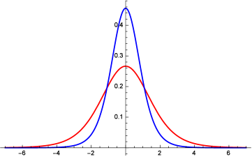
Figure 1: A snapshot at $t=1$ of the FME solution of (58) (red line) and (69) (blue line) initial value problems, with parameters: $d=1$, $\alpha=3/4$.

In the fast diffusion case $\|u\|_{\infty}<\|f\|_{\infty}$ since $C_{\alpha<1}<A_{\alpha<1},\,\,\forall\frac{d}{d+2}<\alpha<1$ as one may prove using (8.1).

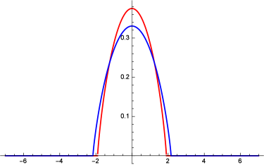
Figure 2: A snapshot at $t=1$ of the PME solution of (58) (red line) and (69) (blue line) initial value problems, with parameters: $d=1$, $\alpha=2.2$.

In the porous medium regime $\|u\|_{\infty}<\|f\|_{\infty}$ up to the threshold value $\alpha_{\textrm{th.}}(d=1)=1.8268$ for which $C_{\alpha>1}=A_{\alpha>1}$ and then $\|u\|_{\infty}>\|f\|_{\infty},\,\,\forall\alpha>1.8268$. The threshold value $\alpha_{\textrm{th.}}$, which depends on the dimension $d$, is determined arithmetically.

6 The concavity of Rényi’s entropy power

Definition 6.1

Let $f:\,\Omega\times(0,\infty)\subset\mathbb{R}^{d}\times(0,\infty)\rightarrow\mathbb{R}^{d}_{+}\times(0,\infty)$ be a p.d.f. in $\mathcal{D}_{\alpha}$. The $\alpha$-weighted Fisher information of $f$ is defined as

$$I_{\alpha}[f](t)=\frac{1}{\int_{\Omega}f^{\alpha}d\mu}\int_{\Omega}\frac{|\nabla f^{\alpha}|^{2}}{f}d\mu,$$ (71)

while the entropy power of $f$ associated to the Rényi entropy $H_{\alpha}$ is defined as

$$\mathcal{N}_{\alpha}[f](t)=\left\{\begin{array}[]{lcc}e^{\left(\frac{2}{d}+(\alpha-1)\right)H_{\alpha}[f](t)}=\left(\int f^{\alpha}d\mu\right)^{-1}\left(\int f^{\alpha}d\mu\right)^{\frac{2}{d(1-\alpha)}},&0<\alpha<\infty,&\alpha\neq 1\\ e^{\frac{2}{d}H_{1}[f](t)},&\alpha=1&\\ \mu(\{x:f(x,t)>0\})^{\frac{2}{d}-1},&\alpha=0.&\end{array}\right.$$ (75)

Proposition 6.2

Let $\Omega=\mathbb{E}^{d}$ be the d-dimensional Euclidean space. The entropy power $\mathcal{N}_{\alpha}$ is a concave function of $t,\,\forall t\in(0,\infty)$ provided that :

$$\frac{d^{2}H_{\alpha}[f](t)}{dt^{2}}\leq\left\{\begin{array}[]{lc}-\frac{d}{(2+d(\alpha-1))}t^{-2}&\textrm{if}\quad\frac{d}{d+2}<\alpha<1\\ &\\ -\frac{d}{(2\alpha-1)^{2}(2+d(\alpha-1))}t^{-2}&\textrm{if}\quad\alpha>1,\end{array}\right.$$ (79)

where the right hand side of the inequality represents the contributions from the global maximum of $H_{\alpha}$.

Proof
Using the nonlinear diffusion equation, a straightforward calculation reveals the connection between $dH_{\alpha}/dt$ and $I_{\alpha}$ expressed by the relation

$$\frac{dH_{\alpha}[f](t)}{dt}=K_{\alpha}^{-1}I_{\alpha}[f](t).$$ (80)

The entropy power is a concave function of time iff

$$\frac{d^{2}\mathcal{N}_{\alpha}[f](t)}{dt^{2}}\leq 0\Longleftrightarrow\left(\frac{2}{d}+(\alpha-1)\right)\left(\frac{d^{2}H_{\alpha}[f](t)}{dt^{2}}+\left(\frac{2}{d}+(\alpha-1)\right)\left(\frac{dH_{\alpha}[f](t)}{dt}\right)^{2}\right)\mathcal{N}_{\alpha}[f](t)\leq 0$$ (81)

or, equivalently when

$$\frac{d^{2}H_{\alpha}[f](t)}{dt^{2}}=K_{\alpha}^{-1}\frac{dI_{\alpha}[f](t))}{dt}\leq-\left(\frac{2}{d}+(\alpha-1)\right)\left(\frac{dH_{\alpha}[f](t)}{dt}\right)^{2}.$$ (82)

Next, we establish the identity

$$\frac{dH_{\alpha}[f](t)}{dt}=\frac{\alpha^{2}K_{\alpha}^{-1}}{(1-2\alpha)\int_{\mathbb{R}^{d}}f^{\alpha}dx}\int_{\mathbb{R}^{d}}f^{2\alpha-1}\Delta\left(\ln f\right)dx.$$ (83)

To do so we rewrite the integral as

$$\int_{\mathbb{R}^{d}}\frac{|\nabla f^{\alpha}|^{2}}{f}dx = \int_{\mathbb{R}^{d}}f^{\alpha-1}\nabla f^{\alpha}\cdot\nabla(\ln f^{\alpha})dx$$ (84)

$$= -\alpha\int_{\mathbb{R}^{d}}f^{\alpha}\left(\nabla f^{\alpha-1}\cdot\nabla(\ln f)+f^{\alpha-1}\Delta(\ln f)\right)$$

$$= \frac{\alpha(1-\alpha)}{(2\alpha-1)}\int_{\mathbb{R}^{d}}\nabla f^{2\alpha-1}\cdot\nabla(\ln f)dx-\alpha\int_{\mathbb{R}^{d}}f^{2\alpha-1}\Delta(\ln f)dx$$

$$= \frac{\alpha^{2}}{(1-2\alpha)}\int_{\mathbb{R}^{d}}f^{2\alpha-1}\Delta(\ln f)dx.$$

The first time derivative of the Rényi entropy satisfies the following upper bounds

$$\frac{dH_{\alpha}[f](t)}{dt}\leq\left\{\begin{array}[]{lc}\frac{d}{(2+d(\alpha-1))}t^{-1}&\textrm{if}\quad\frac{d}{d+2}<\alpha<1\\ &\\ \frac{d}{(2\alpha-1)(2+d(\alpha-1))}t^{-1}&\textrm{if}\quad\alpha>1.\end{array}\right.$$ (88)

To prove this note that the term $\Delta(\ln\hat{f})$ is given by

$$\Delta(\ln\hat{f}(x,t))=-\frac{1}{|1-\alpha|}\frac{2\beta}{t^{2\gamma}}\times\Biggl{\{}\begin{array}[]{lc}\left(1+\beta\frac{x^{2}}{t^{2\gamma}}\right)^{-2}\left[d+(d-2)\beta\frac{x^{2}}{t^{2\gamma}}\right]&\textrm{if}\quad\frac{d}{d+2}<\alpha<1\\ &\\ \left(1-\beta\frac{x^{2}}{t^{2\gamma}}\right)^{-2}\left[d-(d+2)\beta\frac{x^{2}}{t^{2\gamma}}\right]&\textrm{if}\quad\alpha>1\end{array}$$ (92)

and therefore its contribution to the integral is

$$\int_{\mathbb{R}^{d}}\hat{f}^{2\alpha-1}\Delta(\ln\hat{f})dx = -\frac{1}{|1-\alpha|}\frac{2\beta^{1-\frac{d}{2}}|\mathbb{S}_{d-1}|}{t^{2\gamma(1+d(\alpha-1))}}$$ (96)

$$\times \!\!\!\!\!\left\{\begin{array}[]{lcc}\!\!\!\!A_{\alpha<1}^{2\alpha-1}\left[dB(\frac{d}{2},\frac{1}{1-\alpha}-\frac{d}{2})+(d-2)B(1+\frac{d}{2},\frac{\alpha}{1-\alpha}-\frac{d}{2})\right]&\textrm{if}&\frac{d}{d+2}<\alpha<1\\ &\\ \!\!\!\!A_{\alpha>1}^{2\alpha-1}\left[dB(\frac{d}{2},\frac{\alpha}{\alpha-1})-(d+2)B(1+\frac{d}{2},\frac{\alpha}{\alpha-1}+1)\right]&\textrm{if}&\alpha>1.\end{array}\right.$$

Also,

$$\frac{\alpha^{2}}{(1-2\alpha)}\frac{K^{-1}_{\alpha}}{\int_{\mathbb{R}^{d}}f^{\alpha}(x,t)dx}=\frac{\alpha}{2(1-2\alpha)}\frac{(2\alpha+d(\alpha-1))}{(2+d(\alpha-1))}\frac{\beta^{\frac{d}{2}}}{|\mathbb{S}_{d-1}|}t^{d\gamma(\alpha-1)}\times\left\{\begin{array}[]{lcc}\frac{A^{1-2\alpha}_{\alpha<1}}{B(\frac{d}{2},\frac{\alpha}{1-\alpha}-\frac{d}{2})}&\textrm{if}&\frac{d}{d+2}<\alpha<1\\ &\\ \frac{A^{1-2\alpha}_{\alpha>1}}{B(\frac{d}{2},\frac{\alpha}{\alpha-1}+1)}&\textrm{if}&\alpha>1.\end{array}\right.$$ (100)

Substituting (88) into (82) we recover the expected result. $\Box$
Note that in the $\alpha\rightarrow 1^{-}$ limit we reproduce the well-known result valid for the Shannon’s entropy.

Next we prove the concavity of Rény’s power entropy on a different setting. This problem was also studied in [18] but our approach leads to a condition not predicted before. We will need the following lemma.

Lemma 6.3

Let $G$ be defined as

$$G_{\alpha}[f](t)=\int_{\mathbb{R}^{d}}\frac{|\nabla f^{\alpha}|^{2}}{f}dx=\int_{\mathbb{R}^{d}}f|\nabla v|^{2}dx\quad\textrm{where}\quad v=\frac{\alpha}{\alpha-1}f^{\alpha-1}$$ (101)

then

$$\frac{dG_{\alpha}[f](t)}{dt} = -2K_{\alpha}^{-1}\int_{\mathbb{R}^{d}}f^{\alpha}\left(\|\nabla\nabla v\|^{2}+(\alpha-1)(\Delta v)^{2}\right)dx$$ (102)

$$\frac{dI_{\alpha}[f](t)}{dt} = (1-\alpha)K_{\alpha}^{-1}I_{\alpha}^{2}+\frac{1}{\int_{\mathbb{R}^{d}}f^{\alpha}dx}\frac{dG_{\alpha}[f](t)}{dt}.$$ (103)

Proof
Using the porous medium equations for $f,v$ as well as the relation $\nabla f^{\alpha}=f\nabla v$ we have

$$\frac{dG[f](t)}{dt} = \int_{\mathbb{R}^{d}}\left(f_{t}|\nabla v|^{2}+2f_{t}\nabla v(x,t)\cdot\nabla v_{t}\right)dx,\,\,v_{t}=\frac{\partial v}{\partial t}$$ (104)

$$= K_{\alpha}^{-1}\int_{\mathbb{R}^{d}}\left(\Delta f^{\alpha}|\nabla v|^{2}+2f\nabla v\cdot\nabla\left((\alpha-1)v\nabla v+|\nabla v|^{2}\right)\right)dx$$

$$= K_{\alpha}^{-1}\int_{\mathbb{R}^{d}}\left(\Delta f^{\alpha}|\nabla v|^{2}+2(\alpha-1)\left(f|\nabla v|^{2}\Delta v+fv\nabla v\cdot\nabla\Delta v\right)+2f\nabla v\cdot\nabla|\nabla v|^{2}\right)dx$$

$$= K_{\alpha}^{-1}\int_{\mathbb{R}^{d}}\left(\Delta f^{\alpha}|\nabla v|^{2}+2(\alpha-1)\nabla f^{\alpha}\cdot\nabla v\Delta v+2\alpha f^{\alpha}\nabla v\cdot\nabla\Delta v+2\nabla f^{\alpha}\cdot\nabla|\nabla v|^{2}\right)dx$$

$$= K_{\alpha}^{-1}\int_{\mathbb{R}^{d}}\!\!\!\!\left(\left(\Delta f^{\alpha}-2\Delta f^{\alpha}\right)|\nabla v|^{2}-2(\alpha-1)f^{\alpha}\left((\Delta v)^{2}+\nabla v\cdot\nabla\Delta v\right)+2\alpha f^{\alpha}\nabla v\cdot\nabla\Delta v\right)dx$$

$$= K_{\alpha}^{-1}\int_{\mathbb{R}^{d}}\left(f^{\alpha}\left(2\nabla v\cdot\nabla\Delta v-\Delta(|\nabla v|^{2})\right)-2(\alpha-1)f^{\alpha}(\Delta v)^{2}\right)dx$$

$$= -2K_{\alpha}^{-1}\int_{\mathbb{R}^{d}}f^{\alpha}\left(\|\nabla\nabla v\|^{2}+(\alpha-1)(\Delta v)^{2}\right)dx,$$

where partial integrations in the fourth and fifth equalities have been used. Also in the last step the Bochner’s formula in Euclidean space has been applied. Relation (103) is proved using (102). $\Box$

Theorem 6.4

The Rényi entropy power, for self-similar solutions, is concave in t provided that the following inequality is satisfied

$$\int_{\mathbb{R}^{d}}\left(f^{\alpha}(\xi)-Cf^{2\alpha-1}(\xi)\right)d\xi\geq 0,\quad\xi=\frac{x}{t^{\gamma}},\quad C=\frac{1}{\alpha^{2}(1+d(\alpha-1))},$$ (105)

where the equality holds for $\alpha=1$.

Proof
The Rényi entropy power is concave in t iff the condition(82) holds which can be written equivalently as

$$I^{2}_{\alpha}[f](t) \leq d\left(\int_{\mathbb{R}^{d}}f^{\alpha}dx\right)^{-1}\int_{\mathbb{R}^{d}}f^{\alpha}\left(\|\nabla\nabla v\|^{2}+(\alpha-1)(\Delta v)^{2}\right)dx$$ (106)

$$\leq d(1+d(\alpha-1))\left(\int_{\mathbb{R}^{d}}f^{\alpha}dx\right)^{-1}\int_{\mathbb{R}^{d}}f^{\alpha}\|\nabla\nabla v\|^{2}dx$$

$$\leq d(1+d(\alpha-1))J_{\alpha}[f](t),$$

where $\|\nabla\nabla v\|^{2}=\|\textrm{Hess}\,v\|^{2}=\sum_{i,j=1}^{d}(\partial_{ij}v)^{2}$ and we used the identity $\|\textrm{Hess}\,v\|^{2}=\textrm{Tr}\left((\textrm{Hess}\,v)^{2}\right)\geq\left(\textrm{Tr}(\textrm{Hess}\,v)\right)^{2}/d$. Expanding $\|\cdot\|^{2}$ and writing it in terms of $\ln f$ the last integral can be casted into the form

$$\int_{\mathbb{R}^{d}}f^{\alpha}\|\nabla\nabla v\|^{2}dx=\alpha^{2}\int_{\mathbb{R}^{d}}f^{2\alpha-1}\sum_{i,j=1}^{d}\left((\alpha-1)(\partial_{i}\ln f)(\partial_{j}\ln f)+\partial_{ij}^{2}\ln f\right)^{2}dx,$$ (107)

which by applying the Cauchy-Schwarz inequality we get that

$$\int_{\mathbb{R}^{d}}f^{\alpha}\|\nabla\nabla v\|^{2}dx\geq\frac{\alpha^{2}}{d}\left(\int_{\mathbb{R}^{d}}f^{2\alpha-1}dx\right)^{-1}\left(\int_{\mathbb{R}^{d}}f^{2\alpha-1}\left((\alpha-1)|\nabla\ln f|^{2}+\Delta\ln f\right)dx\right)^{2}.$$ (108)

Using the identity

$$\frac{\Delta f^{\alpha}}{f^{\alpha}}=|\nabla\ln f^{\alpha}|^{2}+\Delta\ln f^{\alpha}$$ (109)

we eliminate the $|\nabla\ln f|^{2}$ term from the previous relation and get

$$J_{\alpha}[f](t)\geq\frac{\alpha^{2}}{d}\frac{\left(\int_{\mathbb{R}^{d}}f^{\alpha}\right)}{\left(\int_{\mathbb{R}^{d}}f^{2\alpha-1}\right)}I^{2}_{\alpha}(f)\geq\frac{1}{d(1+d(\alpha-1))}I^{2}_{\alpha}(f).$$ (110)

$\Box$
In 1979, Aronson and Bénilan obtained a second-order differential inequality of the form [1]

$$\sum_{i=1}^{d}\frac{\partial}{\partial x_{i}}\left(\alpha f^{\alpha-2}\frac{\partial f}{\partial x_{i}}\right)=\Delta\left(\frac{\alpha}{\alpha-1}f^{\alpha-1}\right)\geq-\frac{d}{\left(d(\alpha-1)+2\right)t},\quad\alpha>\alpha_{c}:=1-\frac{2}{d},$$ (111)

which applies to all positive smooth solutions of the porous medium equation defined on the whole Euclidean space. In 1986 Li-Yau studied a heat type flow [10] on complete Riemannian manifolds $(M,g)$ with nonnegative Ricci scalar and for any positive function $f$ on M and any $t>0$ they arrived at the following sharp lower bound

$$\Delta(\ln f)\geq-\frac{d}{2t},$$ (112)

pointwise, where $\Delta$ is the Laplace-Beltrami operator on $M$. An extension of the Aronson and Bénilan estimate to the PME flow for all $\alpha>1$ and the FME flow for $\alpha\in(\alpha_{c},1)$ on complete Riemannian manifolds with Ricci scalar bounded from below was given in [11].

In our case these bounds change because our p.d.f. differs from the solution of the PME derived from the gradient flow of the functional [15]

$$E[f](t)=\frac{1}{1-\alpha}\int_{\mathbb{R}^{d}}f^{\alpha}(x,t)dx.$$ (113)

7 Conclusions

In this article we have proved that the p.d.f.’s that maximize Rényi’s entropy under the conditions of finite variance and of zero or non-zero mean are given by a one-parameter family of functions which belong to $S(\mathbb{R}^{d})$ for $\alpha<1$ and to $C^{l}_{0}(\mathbb{R}^{d})$ for $\alpha>1$. This one-parameter family of functions is a global maximum of the entropy and satisfies the non-linear diffusion equation (69). The $\mathcal{L}_{\infty}$ norms of these solutions when compared to the corresponding ones derived from the fast and porous medium diffusion equation initial value problem (58), they appear to behave in a particular way as seen in Figures (1) and (2).

If one considers finite even moments of the random variable $X$, as constraints, and try to solve the corresponding maximization problem then the $S(\mathbb{R})$ solution exists whenever $\hat{f}^{\alpha-1}$ is a complete polynomial of even degree, or equivalently, when all the coefficients $\tilde{\lambda}_{2k+1}$ vanish. In those cases there exists the possibility not to have interception points with the x-axis since the roots come into conjugate complex pairs. The compactly supported solution, under certain conditions, can always be determined.

The concavity of entropy power holds whenever the second time derivative of the entropy varies according to (79) or the function $f^{\alpha}-Cf^{2\alpha-1}$ belongs to $L_{1}(\mathbb{R}^{d})$. It would be more appealing to have a deeper understanding of the origin of the later constraint which at this stage seems to be a requirement for consistency.

8 Acknowledgments

The author would like to thank both J. K. Pachos for the fruitful discussions he had related to this project, and the Department of Physics and Astronomy of the University of Leeds for its hospitality during this visit.

Appendix

Using the two integral formulas [6]

$$\int_{0}^{\infty}x^{\mu-1}(1+x^{2})^{\nu-1}dx = \frac{1}{2}B(\frac{\mu}{2},1-\nu-\frac{\mu}{2}),\quad\textrm{Re}\mu>0,\,\textrm{Re}(\nu+\frac{\mu}{2})<1$$

$$\int_{0}^{1}x^{\mu-1}(1-x^{\lambda})^{\nu-1}dx = \frac{1}{\lambda}B(\frac{\mu}{\lambda},\nu),\quad\textrm{Re}\mu,\,\textrm{Re}\nu,\,\lambda>0,$$ (A.1)

one can prove the following ones, used in section 3,

1. $$\int_{0}^{\infty}x^{\mu-1}(1+x^{2})^{\nu-1}dx=\frac{1}{2}\int_{0}^{1}u^{\frac{\mu}{2}-1}(1-u)^{-\nu-\frac{\mu}{2}}=\frac{1}{2}B(\frac{\mu}{2},1-\nu-\frac{\mu}{2}),$$ (A.2)

   where we made the change of variable $u=x^{2}/(1+x^{2})$.

2. $$\int_{\mathbb{S}_{d-1}}\int_{0}^{\infty}\!\!\!\!\frac{r^{d-1}}{(C(\alpha)+g(\alpha)r^{2})^{\lambda(\alpha)}}dr\,dS=|\mathbb{S}_{d-1}|\frac{C^{\frac{d}{2}-\lambda}}{2g^{\frac{d}{2}}}B(\frac{d}{2},\lambda-\frac{d}{2})\,\,\,\textrm{where}\,\,\,C,g,\lambda>0,\,\,d<2\lambda,$$ (A.3)

   $|\mathbb{S}_{d-1}|=\frac{2\pi^{\frac{d}{2}}}{\Gamma\left(\frac{d}{2}\right)}$ is the volume of the unit ball and $B(x,y)=\Gamma(x)\Gamma(y)/\Gamma(x+y)$ is the Euler’s beta function. The constraint $d<2\lambda$ for $\lambda=1/(1-\alpha)$ allows only values

   $$\alpha_{c_{0}}=1-\frac{2}{d}<\alpha<1\quad\textrm{for}\quad d\geq 3,$$ (A.4)

   while $\alpha_{c_{0}}=0$ for $d=1,2$.

3. $$\int_{\mathbb{S}_{d-1}}\int_{0}^{\infty}\!\!\!\!\!\!\frac{r^{d+1}}{(C(\alpha)+g(\alpha)r^{2})^{\lambda(\alpha)}}dr\,dS=|\mathbb{S}_{d-1}|\frac{C^{\frac{d}{2}+1-\lambda}}{2g^{1+\frac{d}{2}}}B(\frac{d}{2}+1,\lambda-\frac{d}{2}-1)\,\,\textrm{where}\,\,d+2<2\lambda.$$ (A.5)

   The constraint between $d,\,\lambda$ becomes

   $$\alpha_{c_{2}}=1-\frac{2}{d+2}<\alpha<1\quad\textrm{for}\quad d\geq 1.$$ (A.6)

4. The last formula is

   $$\int_{\mathbb{S}_{d-1}}\!\!\int_{0}^{\infty}\!\!\!\!\!r^{d-1}(C(\alpha)-g(\alpha)r^{2})_{+}^{k(\alpha)}dr\,dS=|\mathbb{S}_{d-1}|\frac{1}{2}g(\alpha)^{-\frac{d}{2}}C(\alpha)^{\frac{d}{2}+k(\alpha)}B(\frac{d}{2},k(\alpha)+1)$$

   $$\textrm{when}\quad k(\alpha)>0.$$ (A.7)

Formulas (A.3)-(A.4) are direct consequences of (A.1) and (A.2). Another integral formula [6] used in section 4 is

$$\int_{\mathbb{R}}\frac{x^{m}}{(ax^{2}+2\beta x+c)^{n}} = \frac{(-1)^{m}\pi a^{n-m}b^{m}}{(2n-2)!!(ac-b^{2})^{n-\frac{1}{2}}}$$ (A.11)

$$\times \sum_{k=0}^{[m/2]}\left(\begin{array}[]{c}m\\ 2k\end{array}\right)(2k-1)!!(2n-2k-3)!!\left(\frac{ac-b^{2}}{b^{2}}\right)^{k}$$

$$\textrm{where}\quad ac-b^{2}>0,\,\,0\leq m\leq 2(n-1)$$

and $m,n$ are nonnegative, positive integers respectively.

Identities involving the Euler’s beta function

1. $$\lim_{\rho\rightarrow\infty}\left(\rho^{\frac{s}{2}}B(\frac{s}{2},\rho-\frac{s}{2})\right)=\Gamma\left(\frac{s}{2}\right)$$ (A.12)

   Proof
   The large asymptotic expansion of the ratio of gamma functions [19], is given by

   $$\frac{\Gamma(\rho+a)}{\Gamma(\rho+b)}=\rho^{a-b}\left(1+\frac{(a-b)(a+b-1)}{\rho}+O(\rho^{-2})\right).$$ (A.13)

   Substituting the values $a=-s/2$, $b=0$ in the previous expression and taking the limit $\rho\rightarrow\infty$ we recover the desired result.
   

2. $$d\frac{B(\frac{d}{2},\frac{1}{1-\alpha}-\frac{d}{2})}{B(\frac{d}{2},\frac{\alpha}{1-\alpha}-\frac{d}{2})}+(d-2)\frac{B(1+\frac{d}{2},\frac{\alpha}{1-\alpha}-\frac{d}{2})}{B(\frac{d}{2},\frac{\alpha}{1-\alpha}-\frac{d}{2})} = \frac{d}{\alpha}(2\alpha-1)$$

   $$d\frac{B(\frac{d}{2},\frac{\alpha}{\alpha-1})}{B(\frac{d}{2},\frac{\alpha}{\alpha-1}+1)}-(d+2)\frac{B(1+\frac{d}{2},\frac{1}{\alpha-1}+1)}{B(\frac{d}{2},\frac{\alpha}{\alpha-1}+1)} = \frac{d}{\alpha}.$$ (A.14)

   These are direct consequences of the definition of the Euler’s beta function and the gamma’s function property $\Gamma(x+1)=x\Gamma(x)$.

3. $$B(\frac{1}{2},n-\frac{1}{2}) = \frac{(2n-3)!!}{(2n-2)!!}\pi$$

   $$B(k+\frac{1}{2},n-k-\frac{1}{2}) = (2k-1)!!\frac{(2n-2k-3)!!}{(2n-2)!!}\pi,\quad k\in\mathbb{Z}^{+}$$

   $$B(\frac{1}{2},n+1) = 2^{2n+1}B(n+1,n+1)$$ (A.15)

   Proof
   Use the doubling formula for gamma functions and $\Gamma(n)$ in terms of the double factorial

   $$\Gamma\left(n+\frac{1}{2}\right) = \frac{\sqrt{\pi}}{2^{n}}(2n-1)!!$$

   $$\Gamma(n) = \frac{(2n-2)!!}{2^{n-1}}$$ (A.16)

Proposition 8.1

The function $\Gamma(x)/\Gamma(x+c)$ with $x,c\,\in\mathbb{R}^{+}$ is decreasing in $x$.

Proof It is enough to prove that

$$\frac{d}{dx}\ln\biggl{(}\frac{\Gamma(x)}{\Gamma(x+c)}\biggr{)}=\psi(x)-\psi(x+c)<0.$$ (A.17)

A straightforward computation gives

$$-\ln\biggl{(}1+\frac{c}{x}\biggr{)}-\frac{c}{x(x+c)}\leq\psi(x)-\psi(x+c)\leq-\ln\biggl{(}1+\frac{c}{x}\biggr{)}-\frac{c}{2x(x+c)}<0$$ (A.18)

by using the inequality

$$\ln x-\frac{1}{x}\leq\psi(x)\leq\ln x-\frac{1}{2x}.$$ (A.19)

References

• [1] Aronson, D.G.; Bénilan, P. Régularité des solutions de l’équation des milieux poreux dans $\mathbb{R}^{n}$. C. R. Acad. Sci. Paris. Sér. 1979, A-B 288, 103-105.
• [2] Barenblatt, G.I. On some unsteady motions of a liquid and gas in a porous medium, Akad. Nauk SSSR, Prikl. Mat. Mec., 1952, 16, 67-78.
Barenblatt, G.I. Scaling, Self-Similarity and Intermediate Asymptotics; Cambridge Univ. Press: Cambridge, U.K., 1996.
• [3] Bennett, C.H.; Brassard, G.; Crépeau, C.; Maurer, U.M. Generalized privacy amplification, IEEE Transactions of Information Theory, 1995, 41, 1915-1923.
• [4] Evangelisti, S. Quantum correlations in field theory and integrable systems, Minkowski Institute Press: U.K., 2013.
• [5] Geman, D.; Jedynak, B. An active testing model for tracking roads in satellite images, IEEE Trans. on Pattern Anal. and Machine Intell., 1996, 1, 10-17.
• [6] Gradshteyn, I.S.; Ryzhik, I.M. Table of Integrals, Series, and Products, Academic Press, 5th edition, 1994.
• [7] Havrda M.; Charvát, F. Quantification method of classification processes: concept of structural $\alpha$-entropy, Kybernetika, 1967, 3, 30-35.
• [8] Horodecki, R.; Horodecki, P.; Horodecki, M.; Horodecki, K. Quantum entanglement, Rev. Mod. Phys., 2009, 81, 865-942.
• [9] Jenssen, R.; Hild, K.E.; Erdogmus, D.; Principe, J.C.; Eltoft, T. Clustering using Renyi’s Entropy. In Proceedings of the International Joint Conference on Neural Networks, Portland, OR, 20-24 July 2003; IEEE: Piscataway, NJ, 2003, 1, pp. 523-528.
• [10] Li, P.; Yau, S.T. On the parabolic kernel of the Schrödinger operator, Acta Math., 1986, 56, 153- 201.
• [11] Lu, P.; Ni, N.; Vázquez, L.J.; Villani, C. Local Aronson-Bénilan estimates and entropy formulae for porous medium and fast diffusion equations on manifolds, J. Math. Pures Appl., 2009, 91, 1-19.
• [12] Liberzon, D. Calculus of variations and optimal control theory, Princeton University Press: Princeton, NJ, USA, 2012.
• [13] Lutwak, E.; Yang, D.; Zhang, G. Cramér-Rao and moment-entropy inequalities for Rényi entropy and generalized Fisher information, IEEE Trans. Inform. Theory, 2005, 51, 473-478.
• [14] Johnson, O.; Vignat, C. Some results concerning maximum Rényi entropy distributions, Ann. Inst. H. Poincaré Probab. Statist., 2007, 43, 339-351.
• [15] Otto, F. The geometry of dissipative evolution equations: the porous medium equation, Commun. in Partial Differential Equations, 2001, 26, 101-174.
• [16] Sahoo, P.; Wilkins, V.; Yeager, J. Threshold selection using Reny’is entropy, Pattern Recognition, 1997, 30, 71-84.
• [17] Sankur, B.; Sezgin, M. Image thresholding techniques: a survey over categories, Pattern Recognition, 2001, 34, 1573-1607.
• [18] Savaré, G.; Toscani, G. The concavity of Rényi entropy power, IEEE Trans. Inform. Theory, 2014, 60, 2687-2693.
• [19] Tricomi, F.G.; Erdélyi, A. The asymptotic expansion of a ratio of gamma functions, Pacific J. Math., 1951, 1, 133-142.
• [20] Tsallis, C. Possible generalizations of Boltzmann and Gibbs statistics, J. Stat. Phys., 1988, 52, 479-487.
• [21] Vázquez, J.L. The Porous Medium Equation: Mathematical Theory, Oxford University Press: Oxford, U.K., 2007.
• [22] Zeld’dovich, Ya.B.; Kompaneets, A.S. Towards a theory of heat conduction with thermal conductivity depending on the temperature. Collection of Papers Dedicated to 70th Birthday of Academician A. F. Ioffe, Izd. Akad. Nauk SSSR, Moscow, 1950, 61-71.
• [23] Villani, C. A short proof of the ”concavity of entropy power”, IEEE Trans. Inform. Theory, 2000, 46, 1695-1696.