Abstract: In 2+1 dimensions, Dirac fermions in reducible, i.e. four-component representations of the spinor algebra form the basis of many interesting model field theories and effective descriptions of condensed matter phenomena. This paper explores lattice formulations which preserve the global U$(2N_{f})$ symmetry present in the massless limit, and its breakdown to U($N_{f})\otimes$U($N_{f}$) implemented by three independent and parity-invariant fermion mass terms. I set out generalisations of the Ginsparg-Wilson relation, leading to a formulation of an overlap operator, and explore the remnants of the global symmetries which depart from the continuum form by terms of order of the lattice spacing. I also define a domain wall formulation in 2+1+1$d$, and present numerical evidence, in the form of bilinear condensate and meson correlator calculations in quenched non-compact QED using reformulations of all three mass terms, to show that U($2N_{f}$) symmetry is recovered in the limit that the domain-wall separation $L_{s}\to\infty$. The possibility that overlap and domain wall formulations of reducible fermions may coincide only in the continuum limit is discussed.

Keywords: Lattice Gauge Field Theories, Field Theories in Lower Dimensions, Global Symmetries

1 Introduction

Relativistic fermions moving in two spatial dimensions are at the heart of many interesting issues in theoretical physics, and are increasingly important in effective descriptions of phenomena in condensed matter systems. Let us immediately draw a distinction between so-called irreducible formulations in which the fermion fields $\psi,\bar{\psi}$ are described by two-component spinors, and reducible models which invoke four-component spinors. In the former case, there is no mass term invariant under a discrete parity inversion; gauge theories of irreducible fermions generically manifest a parity anomaly [1, 2, 3], leading to an induced Chern-Simons term endowing the gauge degrees of freedom with mass. Such theories describe excitations with fractional statistics, and form the basis for effective descriptions of the fractional quantum Hall effect [4]. The main focus of this paper, by contrast, will be reducible theories, which like their 4$d$ counterparts admit parity-invariant fermion masses, but whose action is invariant under an enlarged group of global symmetries generated by both $\gamma_{5}$ and the “unused” $\gamma_{3}$. The prototype model involving reducible fermions is QED₃, an asymptotically-free theory with potential non-trivial critical dynamics in the infra-red, and still investigated as a toy model of walking technicolor [5]. Reducible fermions figure in effective descriptions of the spin-liquid phase of quantum antiferromagnets [6, 7], the pseudogap phase of cuprate superconductors [8, 9], and graphene [10, 11, 12].

Once interactions are introduced, reducible 3$d$ fermions may exhibit spontaneous mass generation via formation of a bilinear condensate $\langle\bar{\psi}\psi\rangle\not=0$, entirely analogous to chiral symmetry breaking in QCD. This is manifested in variants of the Gross-Neveu (GN) model [13], in which the basic interaction is a four-fermi contact between scalar or pseudoscalar densities; and also in the Thirring model [14] whose interaction is a contact between two conserved currents, and which shares the global symmetries of QED₃. For GN models the condensate may be studied systematically using an expansion in $1/N_{f}$ where $N_{f}$ is the number of fermion flavors [15], whereas condensate formation in the Thirring model is inherently non-perturbative. In both cases the critical coupling at which the condensate forms is associated with a UV-stable fixed point of the renormalisation group, although the nature of the fixed-point theories remains an open problem [16].

Because field fluctuations near a fixed point can be large, it is natural to explore critical dynamics in 3$d$ using lattice field theory techniques. We immediately confront the issue of how best to formulate the fermion fields. The two traditional approaches which mitigate the species doubling present in naive discretisations are Wilson fermions, which eliminate unwanted species by explicitly breaking important global symmetries, and staggered fermions, which preserve a subgroup of the symmetries by effectively spreading the spinor degrees of freedom over several lattice sites (for an excellent introduction to lattice fermions see chapters 5,7 and 10 of [17]). In a seminal work [18] Coste and Lüscher argued that the Wilson formulation is the more natural for irreducible descriptions, and can be shown to recover the correct parity anomaly (a recent calculation of the mass-dependence of the anomaly in various background fields using Wilson fermions is given in [19]), while the staggered approach naturally leads to a parity-invariant mass term; indeed the relation between staggered fields and the $N_{f}=2$ reducible spinor flavors expected in the continuum limit was given by Burden and Burkitt in [20]. Since the Chern-Simons action is imaginary in Euclidean metric, numerical simulations of $3d$ fermions have to date been restricted almost exclusively to this second case.

To date there have been several papers studying critical behaviour in both GN [15, 21, 22] and Thirring [23, 24, 25] models using numerical simulations of staggered fermions. In general the results support the theoretical prejudice that GN models exhibit a critical point at a coupling $g^{2}\sim O(a)$ (where $a$ is lattice spacing) for all $N_{f}$, with small corrections of O$(1/N_{f})$ to both $g_{c}^{2}$ and the “mean field” critical exponents predicted in the large-$N_{f}$ limit [15]. By contrast, the Thirring model exhibits gap formation only for $N_{f}\leq N_{fc}$, with both exponents and $g_{c}^{2}$ strongly dependent on $N_{f}$ [25]. In the continum, the two models are supposedly distinct. However, recent results obtained with a fermion bag algorithm permitting simulation in the massless limit [26, 27] suggest that in fact the lattice models defined using staggered fermions may actually lie in the same universality class for the minimal case $N_{f}=2$. This somewhat unexpected result is motivation to question the applicability of staggered fermions to problems involving critical fields. For $N$ staggered flavors the global symmetry is U($N)\otimes$U($N$), with $N_{f}=2N$, broken to U($N$) by the generation of a fermion mass. In the long wavelength limit $a\partial\to 0$ this enlarges to the required U($4N)\to$U($2N)\otimes$U($2N$) [20], but there is less reason than usual to trust this restoration once fluctuations on all length scales are important. Other situations where it may be important to reproduce the global symmetry pattern correctly include the infrared behaviour of QED₃, where it has been argued that dynamical mass generation depends on the correct counting of massless degrees of freedom, which include Goldstone modes in a symmetry-broken phase [28], and the role of “half-instantons” in the thermal response of the gapped phase of graphene, which may result in a much reduced value for the critical temperature [29].

This paper explores the application of formulations originally developed to optimise the reproduction of global symmetries in lattice QCD, namely Ginsparg-Wilson (GW) fermions [30] and, principally, domain wall fermions [31, 32], to reducible fermion models in 2+1$d$. After reviewing the relevant symmetries and identifying three distinct but physically equivalent formulations of the mass term in the next section, in Sec. 3 we generalise the GW relation to fermions in 2+1$d$ and identify remnant quasi-global symmetries, which recover the desired U(2$N_{f}$) form only in the continuum limit $a\to 0$. A realisation of the GW symmetries by an overlap operator [33] is given. In Sec. 4 we define a domain wall fermion operator in 2+1+1$d$ which permits the definition of fermi fields localised on domain walls at either end of the newly introduced 3 direction which purport to satisfy the U(2$N_{f}$) symmetry in the limit that the wall separation $L_{s}\to\infty$. An important component of the argument is the reformulation of the three distinct mass terms given in Sec. 2. Sec. 5 presents results from numerical investigations of the $N_{f}=1$ domain wall operator in the context of quenched non-compact QED₃, which permits the use of either weak, strong, or intermediate coupling. While there is no attempt to explore either continuum or thermodynamic limits, we calculate both bilinear condensates (Sec. 5.1) and meson propagators (Sec. 5.2) using each of the three alternative mass terms, and show that in almost all cases as $L_{s}\to\infty$ the results are in accord with a scenario in which U(2) symmetry is broken to U(1)$\otimes$U(1). Interestingly, the most rapid convergence to the U(2)-symmetric limit is obtained for the case of a “twisted” mass term $im\bar{\psi}\gamma_{3}\psi$. For intermediate coupling the results for the condensate $\langle\bar{\psi}\psi\rangle$ are compatible in the massless limit with old results obtained with staggered fermions [35]. Finally in Sec. 6 we present a summary of the findings and an outlook for future investigations. We also discuss the intriguing possibility that for reducible theories of fermions in 2+1$d$ the overlap and domain wall approaches may not coincide except in the continuum limit.

2 Relativistic Fermions in 2+1d

I begin by reviewing the continuum formulation of a gauge theory with fermion fields $\Psi,\bar{\Psi}$ in a reducible representation of the spinor algebra, based on $4\times 4$ Euclidean Dirac matrices $\gamma_{\mu}$ with $\{\gamma_{\mu},\gamma_{\nu}\}=2\delta_{\mu\nu}$, $\mu,\nu=0,1,2$, and having a parity-invariant mass. The weakly-interacting long-wavelength limit of staggered lattice fermions naturally reproduces this formulation with $N_{f}=2$ flavors [20] - in what follows flavor indices are suppressed. The action can be written (for convenience, the necessary $\int d^{3}x$ is omitted in all action definitions)

$$S=\bar{\Psi}D\Psi+m\bar{\Psi}\Psi$$ (1)

where the covariant derivative operator $D$ can be expanded as

$$D=\gamma_{0}D_{0}+\gamma_{1}D_{1}+\gamma_{2}D_{2}=-D^{\dagger}.$$ (2)

This has global symmetries

$$\Psi\mapsto e^{i\alpha}\Psi \bar{\Psi}\mapsto\bar{\Psi}e^{-i\alpha},$$ ; (3)

$$\Psi\mapsto e^{\alpha\gamma_{3}\gamma_{5}}\Psi \bar{\Psi}\mapsto\bar{\Psi}e^{-\alpha\gamma_{3}\gamma_{5}},$$ ; (4)

where $\gamma_{3}$ and $\gamma_{5}$ are two additional traceless, hermitian, and linearly independent 4$\times 4$ matrices which anticommute with all the $\gamma_{\mu}$ (see (8,9) below), and as usual in Euclidean matric $\gamma_{5}\equiv\gamma_{0}\gamma_{1}\gamma_{2}\gamma_{3}$. For fermion mass $m=0$ there are two additional symmetries

$$\Psi\mapsto e^{i\alpha\gamma_{5}}\Psi \bar{\Psi}\mapsto\bar{\Psi}e^{i\alpha\gamma_{5}},$$ ; (5)

$$\Psi\mapsto e^{i\alpha\gamma_{3}}\Psi \bar{\Psi}\mapsto\bar{\Psi}e^{i\alpha\gamma_{3}}.$$ ; (6)

These four rotations generate a global U(2) invariance, which generalises to U$(2N_{f})$ for several flavors. The mass term explicitly breaks the symmetry from U($2N_{f})\to$ U$(N_{f})\otimes$U$(N_{f})$.

It will prove interesting to explore different forms of the mass term, which are simply accessed by changing integration variables in the path integral. Since there is no axial anomaly in $2+1d$, this procedure is straightforward in the continuum and the resulting action describes identical physics. If, however, the representations of the Dirac matrices are tied to the particular form of the underlying lattice, as is the case for staggered fermions or graphene, then due to discretisation effects the mass terms are not equivalent and correspond to distinct patterns of symmetry breaking (see the discussion following eqn. (17) for an example). Let’s recast the continuum action (1) in terms of two two-component spinors $u$ and $d$:

$$S=\bar{u}\tilde{D}u-\bar{d}\tilde{D}d+m\bar{u}u+m\bar{d}d.$$ (7)

where $\tilde{D}=-\tilde{D}^{\dagger}=\sigma_{1}D_{0}+\sigma_{2}D_{1}+\sigma_{3}D_{2}$ and the $\sigma_{i}$ are Pauli matrices. The link with (1) requires the identification

$$\gamma_{0}=\left(\begin{matrix}\sigma_{1}&\cr&-\sigma_{1}\end{matrix}\right);\;\;\gamma_{1}=\left(\begin{matrix}\sigma_{2}&\cr&-\sigma_{2}\end{matrix}\right);\;\;\gamma_{2}=\left(\begin{matrix}\sigma_{3}&\cr&-\sigma_{3}\end{matrix}\right),$$ (8)

implying

$$\gamma_{3}=\left(\begin{matrix}&-i\cr i&\end{matrix}\right);\;\;\gamma_{5}=\left(\begin{matrix}&1\cr 1&\end{matrix}\right);\;\;i\gamma_{3}\gamma_{5}=\left(\begin{matrix}1&\cr&-1\end{matrix}\right).$$ (9)

We now define an important discrete symmetry, parity, here specified for convenience in terms of reversal of all three spacetime axes $x_{\mu}\mapsto-x_{\mu}$ (in general parity must invert an odd number of axes, since flipping an even number is equivalent to a rotation: the Euclidean parity operation which flips just one axis is formally equivalent to the time-reversal operation frequently discussed in condensed matter physics). In fact it can be realised in two ways:

$$\bar{u}\mapsto\bar{d};\;\;\bar{d}\mapsto-\bar{u};\;\;u\mapsto d;\;\;d\mapsto-u;\;\;\;\; \;\Psi\mapsto i\gamma_{3}\Psi;\;\;\bar{\Psi}\mapsto-i\bar{\Psi}\gamma_{3}$$ i.e. (10)

$$\bar{u}\mapsto-i\bar{d};\;\;\bar{d}\mapsto-i\bar{u};\;\;u\mapsto id;\;\;d\mapsto iu;\;\;\;\; \;\Psi\mapsto i\gamma_{5}\Psi;\;\;\bar{\Psi}\mapsto-i\bar{\Psi}\gamma_{5}$$ i.e. (11)

This should be no surprise, since both $\gamma_{3}$ and $\gamma_{5}$ behave identically with respect to the $\gamma_{\mu}$ appearing in (1). In either case the parity operation effectively exchanges the $u$ and $d$ fields, absorbing the sign change of $\tilde{D}$ under $x\to-x$, but keeping the mass term invariant.

Now consider a change of basis

$$\psi={1\over\surd 2}(u+d);\;\;\chi={1\over\surd 2}(-u+d);\;\;\bar{\psi}={1\over\surd 2}(\bar{u}-\bar{d});\;\;\bar{\chi}={1\over\surd 2}(\bar{u}+\bar{d})$$ (12)

in which the action (7) reads

$$S=(\begin{matrix}\bar{\psi}&\bar{\chi}\end{matrix})\left(\begin{matrix}\tilde{D}&-m\cr m&-\tilde{D}\end{matrix}\right)\left(\begin{matrix}\psi\cr\chi\end{matrix}\right)=(\begin{matrix}\bar{\psi}&\bar{\chi}\end{matrix})\left(\begin{matrix}\tilde{D}&-m\cr m&\tilde{D}^{\dagger}\end{matrix}\right)\left(\begin{matrix}\psi\cr\chi\end{matrix}\right).$$ (13)

The parity transformation leaving (13) invariant is equivalent to (10). In terms of four-component spinors the action (13) can be written

$$S=\bar{\Psi}(D-im\gamma_{3})\Psi.$$ (14)

Although the mass term $im\bar{\Psi}\gamma_{3}\Psi$ is still parity invariant, it is now an antihermitian term in the Lagrangian, in contrast to the hermitian mass of (1). Superficially it resembles the twisted mass sometimes used to formulate lattice QCD in 4$d$ [36], though the absence of an anomaly in $2+1d$ permits the term to be flavor singlet. We can also consider a different change of basis

$$\psi={1\over\surd 2}(u+id);\;\;\omega={i\over\surd 2}(u-id);\;\;\bar{\psi}={1\over\surd 2}(\bar{u}+i\bar{d});\;\;\bar{\omega}={i\over\surd 2}(\bar{u}-i\bar{d})$$ (15)

yielding

$$S=(\begin{matrix}\bar{\psi}&\bar{\omega}\end{matrix})\left(\begin{matrix}\tilde{D}&-im\cr-im&-\tilde{D}\end{matrix}\right)\left(\begin{matrix}\psi\cr\omega\end{matrix}\right)=(\begin{matrix}\bar{\psi}&\bar{\omega}\end{matrix})\left(\begin{matrix}\tilde{D}&-im\cr-im&\tilde{D}^{\dagger}\end{matrix}\right)\left(\begin{matrix}\psi\cr\omega\end{matrix}\right),$$ (16)

with this time a parity transformation (11). In terms of four-component spinors (16) can be written

$$S=\bar{\Psi}(D-im\gamma_{5})\Psi;$$ (17)

again, the mass term is parity invariant and antihermitian.

While the three actions (1,14,17) must be equivalent in the continuum, when derived from a lattice system such as a tight-binding model of graphene the terms correspond to physically distinct gapping instabilities at the Dirac cones [37]. The mass term $mS_{h}$ of (1) corresponds to a charge density wave in which electrons preferentially sit on one of the two sub-lattices $A$ or $B$ [38], whereas a linear combination of $m_{3}S_{3}$ (14) and $m_{5}S_{5}$ (17) yields a bond density wave in which electrons are distributed on both $A$ and $B$ sublattices in a Kekulé texture [39].

Note that a mass term proportional to the bilinear $\bar{\Psi}\gamma_{3}\gamma_{5}\Psi$, whether hermitian or antihermitian, is qualitatively different. In terms of two-component spinors the resulting action reads

$$S=(\begin{matrix}\bar{\psi}&\bar{\xi}\end{matrix})\left(\begin{matrix}\tilde{D}+m&\cr&-\tilde{D}-m\end{matrix}\right)\left(\begin{matrix}\psi\cr\xi\end{matrix}\right);$$ (18)

since all elements are proportional to the combination $\tilde{D}+m$ there is no parity operation realisable as a linear transformation on $\Psi,\bar{\Psi}$ which flips the sign of $\tilde{D}$ but leaves the mass term invariant. This corresponds to the non-time-reversal invariant “Haldane mass”, realised in graphene-like systems by alternately circulating currents in adjacent half-unit cells [40].

In summary, there are three linearly independent, physically indistinguishable parity-invariant mass terms available for continuum four-component Dirac fermions in 2+1$d$. We will see that this furnishes a non-trivial test for lattice fermion formulations, such as the domain wall formulation presented in Sec. 4, in which the matrices $\gamma_{3}$ and $\gamma_{5}$ appear in inequivalent ways. Of course, the transformations (12,15) are merely special cases of the rotations (6,5) with $\alpha={\pi\over 4}$, so the physical equivalence of the mass terms is a consequence of U(2) symmetry.

3 Ginsparg-Wilson Relations and the Overlap operator

The Nielsen-Ninomiya theorem [41, 42] famously asserts the impossibility of a lattice fermion formulation with a physical (ie. undoubled) spectrum which simultaneously respects locality, unitarity (or reflection positivity in Euclidean metric) and the existence of a conserved axial charge, expressed in four dimensions via the anticommutator $\{D,\gamma_{5}\}=0$. Ginsparg and Wilson [30] proposed a minimal modification to these criteria for lattice chiral fermions to be viable, namely that chiral symmetry now be constrained by the GW relation

$$\gamma_{5}D+D\gamma_{5}=aD\gamma_{5}D,$$ (19)

where $a$ is the lattice spacing. The non-vanishing right hand side of (19) is effectively an O($a$) contact term for the anticommutator of the propagator $D^{-1}$ with $\gamma_{5}$, which should become unimportant in the long-wavelength limit $aD\to 0$.

The GW relation appropriate to odd-dimensional fermions in irreducible representations of the spinor algebra was investigated by Bietenholz and Nishimura [43], who found that the correct parity anomaly is recovered due to non-invariance of the fermion measure under a “generalised parity” transformation. For the reducible 2+1$d$ theories of interest in this paper the GW relations generalise to:

$$\gamma_{5}D+D\gamma_{5} = aD\gamma_{5}D;$$

$$\gamma_{3}D+D\gamma_{3} = aD\gamma_{3}D;$$ (20)

$$\gamma_{3}\gamma_{5}D-D\gamma_{3}\gamma_{5} = 0.$$ (21)

In addition we require the hermiticity relations

$$\gamma_{3}D\gamma_{3}=\gamma_{5}D\gamma_{5}=D^{\dagger}.$$ (22)

The GW symmetries (19-21) are realised by the overlap operator [33]

$$D^{ov}=a^{-1}(1+\gamma_{3}\mbox{sign}[\gamma_{3}A])=a^{-1}(1+\gamma_{5}\mbox{sign}[\gamma_{5}A])=a^{-1}\left(1+{A\over{(A^{\dagger}A)^{1\over 2}}}\right),$$ (23)

where the matrix $A\equiv aD^{Wils}-1\kern-4.5pt1$, where $D^{Wils}$ is the lattice Dirac operator for orthodox Wilson fermions. It has the properties $\gamma_{5}A\gamma_{5}=\gamma_{3}A\gamma_{3}=A^{\dagger}$ and $i\gamma_{3}\gamma_{5}Ai\gamma_{3}\gamma_{5}=A$, implying $D^{ov}+D^{ov\dagger}=aD^{ov}D^{ov\dagger}=aD^{ov\dagger}D^{ov}$. It is manifest that $\gamma_{3}$ and $\gamma_{5}$ are treated identically in the overlap formalism. A distinct overlap operator, appropriate for irreducible fermions and reproducing the correct parity anomaly, was considered in [44].

Analogously to the situation in 4$d$ [45] the GW relations (19-21) admit the following remnant symmetries, which recover the desired U($2N_{f}$) symmetries (3-6) in the continuum and long-wavelength limits $a\to 0$, $aD\to 0$:

$$\Psi\mapsto e^{\left(i\alpha\gamma_{5}(1-{aD\over 2})\right)}\Psi \bar{\Psi}\mapsto\bar{\Psi}e^{\left(i\alpha(1-{aD\over 2})\gamma_{5}\right)}$$ ;

$$\Psi\mapsto e^{\left(i\alpha\gamma_{3}(1-{aD\over 2})\right)}\Psi \bar{\Psi}\mapsto\bar{\Psi}e^{\left(i\alpha(1-{aD\over 2})\gamma_{3}\right)}$$ ;

$$\Psi\mapsto e^{-\alpha\gamma_{3}\gamma_{5}}\Psi \bar{\Psi}\mapsto\bar{\Psi}e^{\alpha\gamma_{3}\gamma_{5}}.$$ ; (24)

For theories such as the GN and Thirring models defined near a critical point it is not a priori clear that continuum and long-wavelength limits coincide.

To construct mass terms, we define projection operators of two kinds

$$P_{5\pm}={1\over 2}(1\pm\gamma_{5});\;\;P_{3\pm}={1\over 2}(1\pm\gamma_{3}),$$ (25)

and

$$\hat{P}_{5\pm}={1\over 2}(1\pm\hat{\gamma}_{5});\;\;\hat{P}_{3\pm}={1\over 2}(1\pm\hat{\gamma}_{3}),$$ (26)

with

$$\hat{\gamma}_{5}=\gamma_{5}(1-aD);\;\;\hat{\gamma}_{3}=\gamma_{3}(1-aD).$$ (27)

Relations (19-21) may be used to show $\hat{\gamma}_{5}^{2}=\hat{\gamma}_{3}^{2}=1$, so that the $\hat{P}$s are genuine projectors. Importantly, it also follows that

$$D\hat{P}_{3\pm}=P_{3\mp}D;\;\;D\hat{P}_{5\pm}=P_{5\mp}D.$$ (28)

Therefore it makes sense to define two different sets of projected fields:

$$\Psi_{3\pm} = \hat{P}_{3\pm}\Psi;\;\;\bar{\Psi}_{3\pm}=\bar{\Psi}P_{3\mp};$$

$$\Psi_{5\pm} = \hat{P}_{5\pm}\Psi;\;\;\bar{\Psi}_{5\pm}=\bar{\Psi}P_{5\mp},$$ (29)

enabling a decomposition of the kinetic term in two different ways:

$$\bar{\Psi}D\Psi=\bar{\Psi}_{3+}D\Psi_{3+}+\bar{\Psi}_{3-}D\Psi_{3-}=\bar{\Psi}_{5+}D\Psi_{5+}+\bar{\Psi}_{5-}D\Psi_{5-}.$$ (30)

The mass term in this approach is defined in terms of projected fields:

$$m_{h}(\bar{\Psi}_{3-}\Psi_{3+}+\bar{\Psi}_{3+}\Psi_{3-})=m_{h}(\bar{\Psi}_{5-}\Psi_{5+}+\bar{\Psi}_{5+}\Psi_{5-})=m_{h}\bar{\Psi}(1-{aD\over 2})\Psi\equiv m_{h}S_{h}^{GW}.$$ (31)

Although this term only corresponds with the desired mass term in the continuum limit $a\to 0$, the extra O($a$) piece has the same form as the kinetic term, so the overall effect is a benign wavefunction renormalisation. We can also check the effects of the GW symmetries (24), along with the fermion number symmetry (3). With obvious notation, and to $O(\alpha)$:

$$\delta_{1}^{GW}\bar{\Psi}(1-{aD\over 2})\Psi = \delta_{35}^{GW}\bar{\Psi}(1-{aD\over 2})\Psi=0$$ (32)

$$\delta_{3,5}^{GW}\bar{\Psi}(1-{aD\over 2})\Psi = 2i\alpha\bar{\Psi}\gamma_{3,5}(1-{a^{2}D^{\dagger}D\over 4})\Psi$$ (33)

The variation (33) provides the interpolators for the Goldstone modes associated with a spontaneous breaking $\langle\bar{\Psi}(1-{aD\over 2})\Psi\rangle\not=0$; we see there is an O($a^{2}$) correction to the expected continuum forms.

It is interesting to repeat this exercise for the two other parity-invariant mass terms in (14,17). The mass terms constructed from the projected fields are

$$im_{3}(\bar{\Psi}_{3-}\gamma_{3}\Psi_{3+}+\bar{\Psi}_{3+}\gamma_{3}\Psi_{3-})=im_{3}(\bar{\Psi}_{5-}\gamma_{3}\Psi_{5-}+\bar{\Psi}_{5+}\gamma_{3}\Psi_{5+}) = im_{3}\bar{\Psi}\gamma_{3}(1-{aD\over 2})\Psi$$

$$\equiv m_{3}S_{3}^{GW};$$

$$im_{5}(\bar{\Psi}_{3-}\gamma_{5}\Psi_{3-}+\bar{\Psi}_{3+}\gamma_{5}\Psi_{3+})=im_{5}(\bar{\Psi}_{5-}\gamma_{5}\Psi_{5+}+\bar{\Psi}_{5+}\gamma_{5}\Psi_{5-}) = im_{5}\bar{\Psi}\gamma_{5}(1-{aD\over 2})\Psi$$ (34)

$$\equiv m_{5}S_{5}^{GW}.$$

In this case the O($a$) correction does not correspond to an existing term in the action, so the correction may be less benign. Another symptom is that if we label the full Dirac operator including mass terms as ${\cal D}=D+m_{h}S_{1}+m_{3}S_{3}+m_{5}S_{5}$, then

$$\gamma_{3}{\cal D}(m_{h},0,0)\gamma_{3}={\cal D}^{\dagger}(m_{h},0,0);\;\;\;\gamma_{5}{\cal D}(m_{h},0,0)\gamma_{5}={\cal D}^{\dagger}(m_{h},0,0),$$ (35)

but that no such simple relations exist once $m_{3},m_{5}\not=0$.

We find the O($\alpha$) variations of the mass term $S_{3}$ under (24)

$$\delta_{1}^{GW}\bar{\Psi}\gamma_{3}(1-{aD\over 2})\Psi = 0$$

$$\delta_{3}^{GW}\bar{\Psi}\gamma_{3}(1-{aD\over 2})\Psi = 2i\alpha\bar{\Psi}(1-{a^{2}DD^{\dagger}\over 4})(1-{aD\over 2})\Psi$$

$$\delta_{5}^{GW}\bar{\Psi}\gamma_{3}(1-{aD\over 2})\Psi = i\alpha\bar{\Psi}\gamma_{3}\gamma_{5}{a\over 2}(D-D^{\dagger})(1-{aD\over 2})\Psi$$

$$\delta_{35}^{GW}\bar{\Psi}\gamma_{3}(1-{aD\over 2})\Psi = -2\alpha\bar{\Psi}\gamma_{5}(1-{aD\over 2})\Psi$$ (36)

with similar results, mutatis mutandis for variations of $S_{5}$. In all cases the expected expressions for Goldstone interpolators are recovered in the continuum limit. However for $a>0$ there are subtle differences in the effect of the GW variations on the different mass terms; for instance, the two Goldstone interpolators “$\bar{\psi}\psi$” and “$\bar{\psi}\gamma_{5}\psi$” resulting from $\delta_{3}^{GW},\delta_{35}^{GW}$ in (36) have realisations differing by O($a^{2}$) away from the continuum limit. In this sense, full U(2) symmetry is only recovered by overlap fermions as $a\to 0$.

4 Domain Wall Formulation

In this section we set out an alternative route to undoubled U($2N_{f}$)-symmetric fermions using the domain wall approach first introduced by Kaplan [31] and put into the present form by Furman and Shamir [32]. Here we follow the treatment set out in [17]. Define 4-spinor fields $\Psi(x,s)$, $\bar{\Psi}(x,s)$ living on a $4d$ lattice where $x$ denotes the usual 2+1$d$ spacetime coordinates of a lattice site and $s=1,\ldots,L_{s}$ its coordinate along the extra dimension, here labelled 3. The kinetic term in the action is then

$$S^{DW}=\sum_{x,y}\sum_{s,r}\bar{\Psi}(x,s)D^{DW}(x,s|y,r)\Psi(y,r).$$ (37)

with domain wall Dirac operator

$$D^{DW}(x,s|y,r)=\delta_{s,r}D(x|y)+\delta_{x,y}D_{3}^{DW}(s|r).$$ (38)

The first term is the orthodox $2+1d$ Wilson operator

$$D(x|y)={1\over 2}\sum_{\mu=0,1,2}\left[(1-\gamma_{\mu})U_{\mu}(x)\delta_{x+\hat{\mu},y}+(1+\gamma_{\mu})U^{\dagger}_{\mu}(y)\delta_{x-\hat{\mu},y}\right]+(M-3)\delta_{x,y}$$ (39)

with gauge link variables $U_{\mu}(x)$, and $D_{3}^{DW}$ controls hopping in the 3 direction:

$$D_{3}^{DW}(s|s^{\prime})={1\over 2}\bigl{[}(1-\gamma_{3})\delta_{s+1,s^{\prime}}(1-\delta_{s^{\prime},L_{s}})+(1+\gamma_{3})\delta_{s-1,s^{\prime}}(1-\delta_{s^{\prime},1})-2\delta_{s,s^{\prime}}\bigr{]}.$$ (40)

Note there are Dirichlet boundary conditions imposed in direction 3, at $s=1$ and $s=L_{s}$. The inclusion of $D_{3}^{DW}$ explicitly destroys the equivalence of $\gamma_{3}$ and $\gamma_{5}$ in the dynamics described by the action (37), so it will be important to test whether and how this is recovered in practice.

The key idea [31] is that the dynamics generated by (39) and (40), with suitably chosen $M$, results in fermion zeromodes localised on domain walls at $s=1,L_{s}$, which are also respectively $\mp$ eigenmodes of $\gamma_{3}$. The $2+1d$ physics we wish to describe is formulated entirely using these localised modes (the Wilson terms in (39,40) render the would-be zeromodes due to unwanted doubler species non-normalisable in the limit $L_{s}\to\infty$ [31]). In particular we need to define $2+1d$ fermion mass terms corresponding to their continuum counterparts in (1), (14) and (17). To this end, define fermion fields $\psi(x),\bar{\psi}(x)$ living in 2+1$d$:

$$\psi(x) = P_{-}\Psi(x,1)+P_{+}\Psi(x,L_{s});$$

$$\bar{\psi}(x) = \bar{\Psi}(x,L_{s})P_{-}+\bar{\Psi}(x,1)P_{+},$$ (41)

where from now on $P_{\pm}\equiv{1\over 2}(1\pm\gamma_{3})$. We thus consider actions of the form (37) supplemented by three alternative mass terms:

$$m_{h}S_{h}=m_{h}\bar{\psi}\psi = m_{h}[\bar{\Psi}(x,L_{s})P_{-}\Psi(x,1)+\bar{\Psi}(x,1)P_{+}\Psi(x,L_{s})];$$ (42)

$$m_{3}S_{3}=im_{3}\bar{\psi}\gamma_{3}\psi = im_{3}[\bar{\Psi}(x,L_{s})\gamma_{3}P_{-}\Psi(x,1)+\bar{\Psi}(x,1)\gamma_{3}P_{+}\Psi(x,L_{s})];$$ (43)

$$m_{5}S_{5}=im_{5}\bar{\psi}\gamma_{5}\psi = im_{5}[\bar{\Psi}(x,L_{s})\gamma_{5}P_{+}\Psi(x,L_{s})+\bar{\Psi}(x,1)\gamma_{5}P_{-}\Psi(x,1)].$$ (44)

It is interesting to note that $S_{h}$ has the same form as the fermion mass term for domain wall formulations of $3+1d$ physics, and couples fields from opposite walls; $S_{3}$ also couples opposite walls, but $S_{5}$ couples fields living on the same wall.

In the next section we will examine the numerical consequences of the three terms (42-44) and in particular check whether they yield compatible, U(2)-symmetric results in the $L_{s}\to\infty$ limit.

5 Numerical Results

In order to explore the domain wall action (37) supplemented by one of the mass terms (42-44) we have performed quenched simulations of non-compact QED, so that $U_{\mu}(x)=\exp(i\theta_{\mu}(x))$ with the real link variable $\theta$ equilibrated using the Maxwell-like action

$$S_{ncQED}={\beta\over 2}\sum_{\mu\not=\nu}(\Delta^{+}_{\mu}\theta_{\nu}(x)-\Delta^{+}_{\nu}\theta_{\mu}(x))^{2};\;\;\;\mu,\nu=0,1,2.$$ (45)

The dimensionless coupling $\beta\equiv(g^{2}a)^{-1}$, where the dimensionful fermion charge $g$ is the natural scale with which to define physical observables. The continuum limit lies at $\beta\to\infty$. In $2+1d$ QED is an asymptotically-free theory whose infra-red behaviour is still imperfectly understood. Since the non-compact lattice formulation is non-confining, numerical simulations are plagued by the slow fall-off of the photon propagator ($\propto r^{-2}$ for the quenched theory), and the thermodynamic limit is extremely difficult to achieve at weak coupling. Quenched simulations with staggered lattice fermions presented in [35] suggest that chiral symmetry is spontaneously broken in the ground state in the continuum thermodynamic limit, namely (in lattice units $a=1$)

$$\lim_{m\beta\to 0}\lim_{L/\beta\to\infty}\lim_{\beta\to\infty}\langle\bar{\psi}\psi(m)\rangle\not=0.$$ (46)

Lattice sizes up to $80^{3}$ were used in support of this claim.

Away from the continuum limit massless staggered fermions have a manifest U(1)$\otimes$ U(1) global symmetry which spontaneously breaks to U(1) either when an explicit mass is introduced or a chiral condensate of the form (46) develops. Only in the continuum limit can this pattern enlarge to the expected U($2N_{f})\to$U($N_{f})\otimes$U($N_{f}$), with $N_{f}=2$ [20]. The main aim of this study is not to verify (46) for domain wall fermions, but rather to test the restoration of the correct symmetry breaking pattern, with $N_{f}=1$, as $L_{s}\to\infty$. To this end we have performed simulations on system sizes $24^{3}\times L_{s}$, with couplings $\beta=0.5$, 1.0 and 2.0, corresponding respectively to strong, intermediate and weak coupling regimes. Throughout the domain wall fermion mass $M$ in (39) was set to 0.9 (physical quantities are expected to be $M$-independent; §reflection positivity requires $0<M<1$), and unless otherwise stated the masses $m_{h},m_{3},m_{5}$ in (42-44) to 0.01. For convenience a hybrid Monte Carlo algorithm was used to generate the $\{\theta\}$ ensembles, with 100 trajectories of average length 1.0 between measurements; a much more efficient Fourier-space method was employed in the original study [35].

5.1 Bilinear Condensates

First we explore bilinear condensates generically defined by $\langle\bar{\psi}\Gamma_{i}\psi\rangle\equiv\partial\ln{\cal Z}/\partial m_{i}$, where $m_{i}\in\{m_{h},m_{3},m_{5}\}$. These form in response either to $m_{i}\not=0$ or in the thermodynamic limit to strong dynamics. For the latter case in the limit $m_{i}\to 0$ all three condensates should be equal if U(2) symmetry is manifest. It is not obvious that this will occur for the action (37), both because of the Wilson terms inherent in (39,40), and because $\gamma_{3}$ and $\gamma_{5}$ do not appear in (37) on an equal footing. By hypothesis, however, U(2) symmetry should be recovered as $L_{s}\to\infty$.

To begin, we present results obtained using a spatial point source on a configuation generated at $\beta=0.5$ (in fact, the numbers result from averaging over 10 spatial sources); the systematics are easiest to expose at the strongest coupling. Note from (42-44) that each condensate gets contributions from two terms: for $\langle\bar{\psi}\psi\rangle$ and $i\langle\bar{\psi}\gamma_{3}\psi\rangle$ the two terms arise from four-dimensional propagators running from $s=1$ to $L_{s}$ and $L_{s}$ to 1 respectively; for $i\langle\bar{\psi}\gamma_{5}\psi\rangle$ each contribution is from a propagator starting and ending on the same domain wall. Within the working numerical precison each contribution is the complex conjugate of the other, so the sum is real. However, it turns out the imaginary component parametrises the approach to the U(2)-symmetric limit. Define $i\langle\bar{\Psi}(1)\gamma_{3}\Psi(L_{s})\rangle={i\over 2}\langle\bar{\psi}\gamma_{3}\psi\rangle_{L_{s}}+i\Delta_{h}(L_{s})$ (where the first term is real, and the spatial coordinate $x$ is suppressed), and then write:

$${1\over 2}\langle\bar{\psi}\psi\rangle_{L_{s}} = {i\over 2}\langle\bar{\psi}\gamma_{3}\psi\rangle_{L_{S}\to\infty}+\Delta_{h}(L_{s})+\epsilon_{h}(L_{s});$$ (47)

$${i\over 2}\langle\bar{\psi}\gamma_{3}\psi\rangle_{L_{s}} = {i\over 2}\langle\bar{\psi}\gamma_{3}\psi\rangle_{L_{S}\to\infty}+\epsilon_{3}(L_{s});$$ (48)

$${i\over 2}\langle\bar{\psi}\gamma_{5}\psi\rangle_{L_{s}} = {i\over 2}\langle\bar{\psi}\gamma_{3}\psi\rangle_{L_{S}\to\infty}+\epsilon_{5}(L_{s}).$$ (49)

The residuals $\Delta_{h}$ and $\epsilon_{i}$ must vanish for a U(2)-invariant limit.

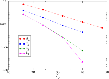
Figure 1: Residual errors as a function of $L_{s}$ for bilinear condensates evaluated using point spatial sources on $24^{3}$ at $\beta=0.5$.

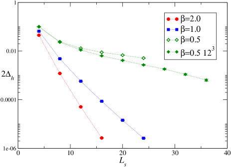
Figure 2: Residual error $2\Delta_{h}(L_{s})$ evaluated for various $\beta$ using a stochastic estimator on $24^{3}$.

Fig. 1 plots the residuals for $L_{s}=16,\ldots,40$; note that $\Delta_{h}$ is measured directly as the imaginary component of $i\langle\bar{\psi}\gamma_{3}\psi\rangle$ using just the $+$ components of $\Psi,\bar{\Psi}$, while to estimate the $\epsilon_{i}$ the value of $i\langle\bar{\psi}\gamma_{3}\psi\rangle_{L_{s}\to\infty}$ is taken to be that measured at $L_{s}=48$. Several features are apparent:

• The dominant correction by almost an order of magnitude is $\Delta_{h}$, which contributes to the hermitian condensate $\langle\bar{\psi}\psi\rangle$ but not, as a result of the twist, to the antihermitian $i\langle\bar{\psi}\gamma_{3,5}\psi\rangle$. Indeed, at the weakest coupling $\beta=2.0$ $\Delta_{h}$ is the only residual large enough to measure.

• All residuals decay approximately as $\exp(-cL_{s})$, consistent with U(2) symmetry restoration as $L_{s}\to\infty$.

• $\epsilon_{3}$ and $\epsilon_{5}$ are practically identical – the disparity in Fig. 1 at $L_{s}=40$ probably results from uncertainty in the determination of $i\langle\bar{\psi}\gamma_{3}\psi\rangle_{L_{S}\to\infty}$. This is striking since the underlying structures in terms of four-dimensional propagators are quite distinct.

Of course, we should not draw universal conclusions from a single gauge configuration, particularly since the bilinear condensates display strong intermittent upward fluctuations across a gauge ensemble. Fig. 2 shows $\Delta_{h}(L_{s})$ evaluated for 1200 ($24^{3}$) or 2400 ($12^{3}$) measurements of $i\langle\bar{\psi}\gamma_{3}\psi\rangle$ at the three couplings explored (for $L_{s}\geq 16$ O(500) measurements were made at the strongest coupling $\beta=0.5$ on $24^{3}$) using a stochastic noise vector $\eta(x)$; to faithfully implement the projectors $P_{\pm}$ in (43) the same $\eta$ is chosen for all spin components in the trace. Reassuringly, for $L_{s}\raisebox{-2.15277pt}{$\ \stackrel{{\scriptstyle\textstyle>}}{{\textstyle\sim}}\ $}8$ the exponential behaviour $\Delta_{h}\propto e^{-cL_{s}}$ persists, with decay constant $c$ decreasing as the coupling increases. Comparison of the $\beta=0.5$ results also shows $c$ is in general also volume-dependent. Although not investigated here, we also expect $c$ to depend on the Lagrangian parameter $M$. There is no reason to doubt, however, that the residuals will eventually become an insignificant systematic as $L_{s}\to\infty$.

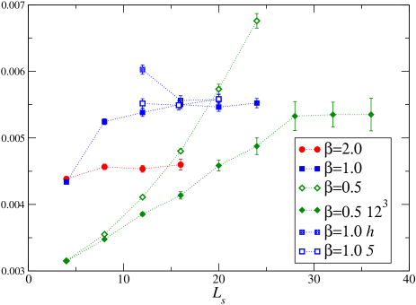
Figure 3: Bilinear condensate $i\langle\bar{\psi}\gamma_{3}\psi\rangle$ for various $\beta$ as a function of $L_{s}$. Results for $\langle\bar{\psi}\psi\rangle$ and $i\langle\bar{\psi}\gamma_{5}\psi\rangle$ at $\beta=1.0$ are also shown.

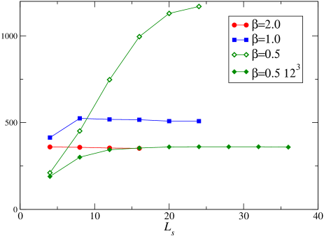
Figure 4: Average number of conjugate gradient iterations per measurement required for the data of Figs. 2,3.

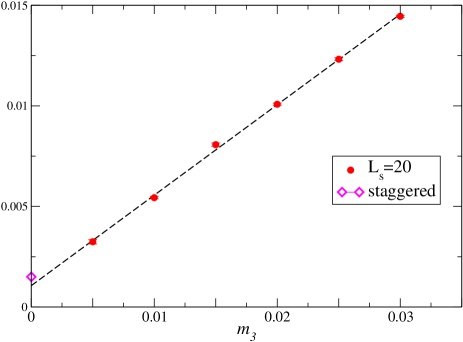
Figure 5: $i\langle\bar{\psi}\gamma_{3}\psi\rangle$ vs. symmetry-breaking mass $m_{3}$ at $\beta=1.0$ on $24^{3}\times 20$. The diamond shows the corresponding observable extrapolated to the chiral limit using staggered fermions [35].

Results for the condensate $i\langle\bar{\psi}\gamma_{3}\psi\rangle$, which as a result of the twist does not include effects of the dominant residual $\Delta_{h}$, are shown in Fig. 3. With the use of a stochastic estimator a conjugate gradient residual of $10^{-12}$ per (four-dimensional) lattice site and spin component sufficed. As a function of $L_{s}$ the results plateau essentially once $\Delta_{h}/|\langle\bar{\psi}\gamma_{3}\psi\rangle|$ is smaller than the statistical error confirming the trends of Fig. 2: this occurs for $L_{s}\raisebox{-2.15277pt}{$\ \stackrel{{\scriptstyle\textstyle>}}{{\textstyle\sim}}\ $}8$ for $\beta=2.0$ and $L_{s}\raisebox{-2.15277pt}{$\ \stackrel{{\scriptstyle\textstyle>}}{{\textstyle\sim}}\ $}16$ for $\beta=1.0$. At the strongest coupling $\beta=0.5$ the available numerical resources have not permitted this regime to be probed on the reference $24^{3}$ volume; however data taken on $12^{3}$ eventually plateau for $L_{s}\raisebox{-2.15277pt}{$\ \stackrel{{\scriptstyle\textstyle>}}{{\textstyle\sim}}\ $}28$. Based on the $\Delta_{h}$ data from Fig. 2 we might guess the $\beta=0.5$, $24^{3}$ plateau may set in for $L_{s}\approx 40$.

Fig. 3 also shows results for the other bilinear condensates $\langle\bar{\psi}\psi\rangle$ ($h$) and $i\langle\bar{\psi}\gamma_{5}\psi\rangle$ ($5$) for $\beta=1.0$, showing that within statistical errors they become consistent with $i\langle\bar{\psi}\gamma_{3}\psi\rangle$ for $L_{s}\raisebox{-2.15277pt}{$\ \stackrel{{\scriptstyle\textstyle>}}{{\textstyle\sim}}\ $}20$. The impact of the $\Delta_{h}$ residual on $\langle\bar{\psi}\psi\rangle$ is clearly discernable, and suggests it is not the optimal choice for systematic studies of chiral symmetry breaking. However, with this level of precision there is no reason not to suppose U(2) symmetry is eventually restored. Fig. 4 shows the number of conjugate gradient iterations required for each fermion matrix inversion is roughly constant once the plateau is reached, implying that the numerical effort needed scales linearly with $L_{s}$ as the U(2)-symmetric limit is approached.

Finally, Fig. 5 plots $i\langle\bar{\psi}\gamma_{3}\psi\rangle$ as a function of $m_{3}$ at $\beta=1.0$ on $24^{3}\times 20$. The data can be plausibly extracted linearly to the chiral limit $m_{3}\to 0$ to yield a non-vanishing intercept, consistent with the hypothesis that chiral symmetry is indeed spontaneously broken (though at this stage no thermodynamic or continuum limit is taken). Also shown is the staggered fermion condensate ${1\over 2}\langle\bar{\chi}\chi\rangle$ (ie. normalised to $N_{f}=1$) on the same spatial volume estimated from Fig. 7 of [35]. The values are close enough to be plausibly consistent, but in any case provide reassurance first that the domain wall fermion data do not contain significant contributions from doubler species, and secondly that the explicit chiral symmetry-breaking violation by the Wilson terms in (39) is mitigated in the domain wall approach. Of course, since there are as-yet unquantified renormalisations of both elementary fields and composite operators, these considerations strictly require a continuum limit to be taken.

5.2 Meson Propagators

Next we turn attention to correlations between mesonic operators $\bar{\psi}\Gamma\psi$ at different spacetime points, with $\Gamma\in\{\gamma_{5},\gamma_{3},1\kern-4.5pt1,i\gamma_{3}\gamma_{5}\}$ all yielding spin-0 states, two with positive parity and two negative. We again focus on the recovery of U(2) symmetry as $L_{s}\to\infty$. A similar analysis for staggered fermions in the continuum limit of non-compact QED₃ was presented in [46]. We begin by listing two important identities of the 2+1+1$d$ fermion propagator $S(m_{i};x,s;y,s^{\prime})=\langle\Psi(x,s)\bar{\Psi}(y,s^{\prime})\rangle$, which follow directly from (37) and have been checked numerically on small lattices:

$$\gamma_{5}S(m_{h},m_{3},m_{5};x,s;y,s^{\prime})\gamma_{5} \equiv S^{\dagger}(m_{h},m_{3},-m_{5};y,s^{\prime};x,s);$$ (50)

$$\gamma_{3}S(m_{h},m_{3},m_{5};x,s;y,s^{\prime})\gamma_{3} \equiv S^{\dagger}(m_{h},-m_{3},m_{5};y,\bar{s}^{\prime};x,\bar{s}).$$ (51)

Here $x$ denotes the coordinate in 2+1$d$ and $s$ that in the 3rd direction, $\bar{s}\equiv L_{s}-s+1$, and the dagger acts on Dirac indices. In what follows a mass parameter $m_{i}$ is omitted from the argument list if it takes the value zero. The identities (50,51) are of course crucial for the efficient calculation of timeslice correlators with a minimal number of matrix inversions, although there will be instances where a further inversion with the sign of the mass term $m_{3,5}$ reversed is needed. The contrast with relations (35) for overlap fermions, which away from the continuum limit only hold for $m_{3}=m_{5}=0$ should be noted. As will be demonstrated, in the limit $L_{s}\to\infty$ two further approximate relations become valid:

$$\gamma_{3}S(m_{3};x,s;y,s^{\prime})\gamma_{3} \approx -S^{\dagger}(m_{3};y,\bar{s}^{\prime};x,\bar{s})\;\mbox{for}\;s^{\prime}=\bar{s};$$

$$\gamma_{3}S(m_{3};x,s;y,s^{\prime})\gamma_{3} \approx S^{\dagger}(m_{3};y,\bar{s}^{\prime};x,\bar{s})\;\mbox{for}\;s^{\prime}=s,$$ (52)

and equivalent ones for $3\leftrightarrow 5$.

Now consider the pion correlator $C_{5}(x)=\langle\bar{\psi}(0)\gamma_{5}\psi\bar{\psi}(x)\gamma_{5}\psi(x)\rangle$. Under the parity definition (10) this state has $J^{P}=0^{-}$. Using the definition (41) and ignoring the overall minus sign from the Grassmann nature of $\Psi,\bar{\Psi}$, we deduce the following relation in terms of 2+1+1$d$ propagators

$$C_{5}(x) = {\rm tr}\Bigl{[}P_{+}S(m_{i};x,L_{s};0,L_{s})P_{-}\gamma_{5}P_{+}S(m_{i};0,L_{s};x,L_{s})P_{-}\gamma_{5}$$ (53)

$$+ P_{-}S(m_{i};x,1;0,1)P_{+}\gamma_{5}P_{-}S(m_{i};0,1;x,1)P_{+}\gamma_{5}$$

$$+ P_{-}S(m_{i};x,1;0,L_{s})P_{-}\gamma_{5}P_{+}S(m_{i};0,L_{s};x,1)P_{+}\gamma_{5}$$

$$+ P_{+}S(m_{i};x,L_{s};0,1)P_{+}\gamma_{5}P_{-}S(m_{i};0,1;x,L_{s})P_{-}\gamma_{5}\Bigr{]}.$$

It’s natural in this formalism to have projectors $P_{\pm}$ sandwiching the fermion propagators – they are the bridge, both formally and in the code, between the 4$d$ and 3$d$ worlds.

Now specialise to the case of mass term $S_{h}$, and use the identity (50), along with translational invariance in 3$d$, to arrive at

$$C_{5}^{h}(x) = {\rm tr}\Bigl{[}S(m_{h};0,L_{s};x,L_{s})P_{-}S^{\dagger}(m_{h};0,L_{s};x,L_{s})P_{+}$$ (54)

$$+ S(m_{h};0,1;x,1)P_{+}S^{\dagger}(m_{h};0,1;x,1)P_{-}$$

$$+ S(m_{h};0,1;x,L_{s})P_{-}S^{\dagger}(m_{h};0,1;x,L_{s})P_{-}$$

$$+ S(m_{h};0,L_{s};x,1)P_{+}S^{\dagger}(m_{h};0,L_{s};x,1)P_{+}\Bigr{]}$$

$$\equiv C^{h-+}(x)+C^{h+-}(x)+C^{h--}(x)+C^{h++}(x).$$ (55)

This has the familiar look of a pion correlator (ie. positive definite terms of the form $SS^{\dagger}$) apart from the projectors, and is clearly calculable with two sources, one located at $s=1$ and the other at $s=L_{s}$. In the abbreviated form (55) note that $-+$ and $+-$ correlators involve fermion propagators linking a domain wall to itself, whereas for $--$ and $++$ the propagators run between the walls.

Next consider the $0^{+}$ correlator $C_{3}^{h}(x)=\langle\bar{\psi}(0)\gamma_{3}\psi\bar{\psi}(x)\gamma_{3}\psi(x)\rangle$. This produces an expression with a different 4$d$ spacetime structure, but which with the help of (51) can be rearranged to coincide exactly with (54):

$$C_{3}^{h}(x) = {\rm tr}\Bigl{[}P_{-}S(m_{h};x,1;0,L_{s})P_{-}\gamma_{3}P_{-}S(m_{h};0,1;x,L_{s})P_{-}\gamma_{3}$$ (56)

$$+ P_{-}S(m_{h};x,1;0,1)P_{+}\gamma_{3}P_{+}S(m_{h};0,L_{s};x,L_{s})P_{-}\gamma_{3}$$

$$+ P_{+}S(m_{h};x,L_{s};0,L_{s})P_{-}\gamma_{3}P_{-}S(m_{h};0,1;x,1)P_{+}\gamma_{3}$$

$$+ P_{+}S(m_{h};x,L_{s};0,1)P_{+}\gamma_{3}P_{+}S(m_{h};0,L_{s};x,1)P_{+}\gamma_{3}\Bigr{]}$$

$$= C^{h--}(x)+C^{h+-}(x)+C^{h-+}(x)+C^{h++}(x)\equiv C_{5}^{h}(x).$$

These two states are thus exactly degenerate if the hermitian mass term $S_{h}$ is chosen.

The same methods can be used for the correlators

$$C_{1}(x) = \langle\bar{\psi}(0)\psi(0)\bar{\psi}(x)\psi(x)\rangle;$$

$$C_{35}(x) = \langle\bar{\psi}(0)i\gamma_{3}\gamma_{5}\psi(0)\bar{\psi}(x)i\gamma_{3}\gamma_{5}\psi(x)\rangle,$$ (57)

which are respectively $0^{+}$ and $0^{-}$ to show

$$C_{1}^{h}(x)=C_{35}^{h}(x) = {\rm tr}\Bigl{[}S(m_{h};0,1;x,L_{s})\gamma_{3}P_{-}S^{\dagger}(m_{h};0,1;x,L_{s})P_{-}\gamma_{3}$$ (58)

$$+ S(m_{h};0,L_{s};x,L_{s})\gamma_{3}P_{-}S^{\dagger}(m_{h};0,L_{s};x,L_{s})P_{+}\gamma_{3}$$

$$+ S(m_{h};0,1;x,1)\gamma_{3}P_{+}S^{\dagger}(m_{h};0,1;x,1)P_{-}\gamma_{3}$$

$$+ S(m_{h};0,L_{s};x,1)\gamma_{3}P_{+}S^{\dagger}(m_{h};0,L_{s};x,1)P_{+}\gamma_{3}\Bigr{]}$$

$$= C^{h--}(x)-C^{h-+}(x)-C^{h+-}(x)+C^{h++}(x).$$

Therefore these two states are also degenerate, but distinct from $\bar{\psi}\gamma_{3}\psi$ and $\bar{\psi}\gamma_{5}\psi$ in (54). Assuming the primitive correlators $C^{h\pm\pm}$ are all positive definite, then $|C_{5}^{h}|=|C_{3}^{h}|>|C_{1}^{h}|=|C_{35}^{h}|$. If the symmetry breaking in the direction of $S_{3}$ is spontaneous this is consistent with U(2)$\rightarrow$U(1)$\otimes$U(1) yielding two light pseudo-Goldstone modes interpolated by $\bar{\psi}\gamma_{5}\psi$ and $\bar{\psi}\gamma_{3}\psi$. Had we instead chosen (11) as the definition of parity, then the assignments of the two Goldstone states would be reversed so that $\bar{\psi}\gamma_{5}\psi$ is now $0^{+}$ and $\bar{\psi}\gamma_{3}\psi$ $0^{-}$. However, the overall picture of a Goldstone $0^{\pm}$ doublet and a non-Goldstone $0^{\pm}$ doublet remains unaltered.

The picture is more interesting when the mass term $S_{3}$ is considered. The correlator $C_{5}^{3}=C^{3-+}+C^{3+-}+C^{3--}+C^{3++}$ in analogy to (54,55), but for $C_{3}^{3}$ we find

$$C_{3}^{3}(x) = {\rm tr}\Bigl{[}S(m_{3};0,1;x,L_{s})P_{-}S^{\dagger}(-m_{3};0,1;x,L_{s})P_{-}$$ (59)

$$+ S(m_{3};0,1;x,1)P_{+}S^{\dagger}(-m_{3};0,1;x,1)P_{-}$$

$$+ S(m_{3};0,L_{s};x,L_{s})P_{-}S^{\dagger}(-m_{3};0,L_{s};x,L_{s})P_{+}$$

$$+ S(m_{3};0,L_{s};x,1)P_{+}S^{\dagger}(-m_{3};0,L_{s};x,1)P_{+}\Bigr{]}$$

$$\equiv \tilde{C}^{3--}(x)+\tilde{C}^{3+-}(x)+\tilde{C}^{3-+}(x)+\tilde{C}^{3++}(x).$$ (60)

The expression (60) is similar in form to (56) but requires twice the number of matrix inversions to evaluate. However, use of the large-$L_{s}$ approximations (52) gives

$$C_{3}^{3}(x)\approx-C^{3--}(x)+C^{3+-}(x)+C^{3-+}(x)-C^{3++}(x).$$ (61)

Similarly we find

$$C_{1}^{3}(x) \approx -C^{3--}(x)-C^{3++}(x)-C^{3-+}(x)-C^{3+-}(x);$$ (62)

$$C_{35}^{3}(x) = C^{3--}(x)+C^{3++}(x)-C^{3-+}(x)-C^{3+-}(x).$$ (63)

This suggests that the Goldstone modes are now interpolated by $\bar{\psi}\psi$ ($0^{+}$) and $\bar{\psi}\gamma_{5}\psi$ ($0^{-}$), consistent with the variation of $S_{3}$ under (3-6), but that the U(2)$\rightarrow$U(1)$\otimes$U(1) pattern will now only be recovered in the limit $L_{s}\to\infty$.

Finally, for mass term $S_{5}$ we have

$$C_{5}^{5}(x) \approx C^{5-+}(x)+C^{5+-}(x)-C^{5--}(x)-C^{5++}(x);$$ (64)

$$C_{3}^{5}(x) = C^{5-+}(x)+C^{5+-}(x)+C^{5--}(x)+C^{5++}(x);$$ (65)

$$C_{1}^{5}(x) = -C^{5-+}(x)-C^{5+-}(x)+C^{5--}(x)+C^{5++}(x);$$ (66)

$$C_{35}^{5}(x) \approx -C^{5-+}(x)-C^{5+-}(x)-C^{5--}(x)-C^{5++}(x);$$ (67)

the apparent contradiction with the expected identification of $\bar{\psi}\psi$ ($0^{+}$) and $\bar{\psi}\gamma_{3}\psi$ ($0^{-}$) (using either the symmetries (3-6) or the change of variables (15)) as Goldstone interpolators will be further discussed below.

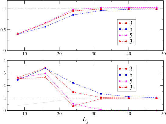
Figure 6: Ratio $\sum_{t=0}^{23}|C/C^{3\pm-}|$ vs. $L_{s}$ for $C=C^{+-}$ (top) and $C=C^{--}$ (bottom) for $\beta=0.5$ on $24^{3}$. The key denotes the mass term used.

We now present numerical results for the primitive correlators $C^{\pm\pm}(x)$. It is clear the recovery of U(2) symmetry hinges on the validity of the approximation (52). As in Sec. 5.1, the first test uses the numerically most demanding system of $\beta=0.5$ on $24^{3}\times L_{s}$, with fermion mass $m_{i}=0.01$. For a single equilibrated configuration we calculated $C^{+-}$ and $C^{--}$, and where relevant their negative mass counterparts $\tilde{C}^{\pm-}$, using five randomly chosen sources with $s=0$. Using $C^{3\pm-}(L_{s}=48)$ as a reference point, the ratio $\sum_{t=0}^{23}C(L_{s})/C^{3\pm-}(48)$ is plotted as a function of $L_{s}$ in Fig. 6 for mass terms $m_{3}S_{3}$, $m_{h}S_{h}$, $m_{5}S_{5}$, along with the same quantity evaluated for $|\tilde{C}^{3}|$ (labeled “3-” in the plot). It is apparent that $C^{3\pm-}$ has reached its large-$L_{s}$ limit by $L_{s}\approx 40$, but that $C^{h\pm-}$ converges rather more slowly. Most importantly, $C^{3+-}$ is indistinguishable from $\tilde{C}^{3+-}$, whereas $\tilde{C}^{3--}$ actually changes sign around $L_{s}\approx 25$ and by $L_{s}\approx 40$ is practically equal to $-C^{3--}$, consistent with (52). The correlators $C^{5\pm-}$ do not, however, fit the same pattern; $C^{5+-}$ lies systematically above $C^{3+-}$, while $C^{5--}\to 0$ as $L_{s}\to\infty$.

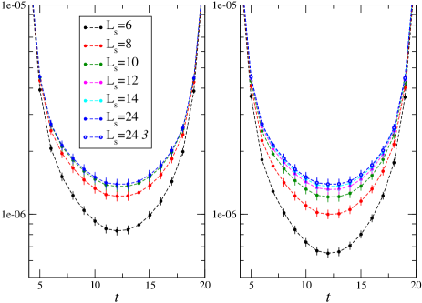
Figure 7: Primitive timeslice correlators $C^{3+-}(t)$ (left) and $C^{h+-}(t)$ (right) for various $L_{s}$ with $\beta=1.0$, $m=0.01$ on $24^{3}$.

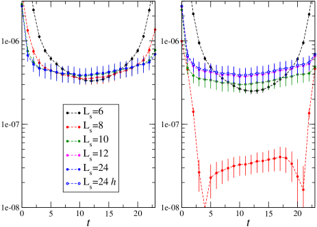
Figure 8: Same as Fig. 7 but for $C^{3--}(t)$ (left) and $|\tilde{C}^{3--}(t)|$ (right).

This picture is confirmed by a study of 500 configurations at $\beta=1.0$, $m_{i}=0.01$ on $24^{3}$. Only the components $C^{\pm-}$, which are manifestly real, are calculated; the counterparts $C^{\mp+}$ are identical, and the correlators $\tilde{C}^{\pm\mp}$ requiring an inversion with a negative fermion mass recover these properties as $L_{s}\to\infty$. To focus on systematic effects the same ensemble was used for each $L_{s}$ – the resulting statistical errorbars show the expected evidence of autocorrelation between timeslices. Fig. 7 compares $C^{3+-}$ with $C^{h+-}$; $C^{3+-}$ converges to its large-$L_{s}$ limit for $L_{s}\raisebox{-2.15277pt}{$\ \stackrel{{\scriptstyle\textstyle>}}{{\textstyle\sim}}\ $}12$, whereas $C^{h+-}$ converges somewhat more slowly, requiring $L_{s}\raisebox{-2.15277pt}{$\ \stackrel{{\scriptstyle\textstyle>}}{{\textstyle\sim}}\ $}16$. Crucially though, by $L_{s}=24$ the two are indistinguishable. Fig. 8 confirms that after a sign change occuring for $L_{s}\approx 8$ then $\lim_{L_{s}\to\infty}\tilde{C}^{3--}=-C^{3--}$, and that both also coincide in magnitude with $C^{h--}$ for $L_{s}\raisebox{-2.15277pt}{$\ \stackrel{{\scriptstyle\textstyle>}}{{\textstyle\sim}}\ $}24$. We have thus demonstrated that the mass terms $S_{h}$ via relations (56,58), and $S_{3}$ via (60-63), must yield equivalent meson spectra as $L_{s}\to\infty$.

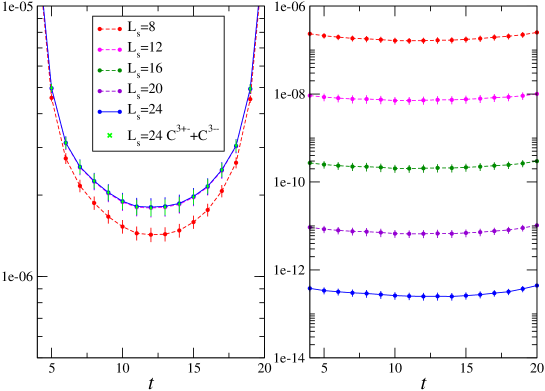
Figure 9: Same as Fig. 7 but for $C^{5+-}(t)$ (left) and $C^{5--}(t)$ (right). Also shown is the combination $C^{3+-}(t)+C^{3--}(t)$ for $L_{s}=24$.

Finally Fig. 9 shows the primitive correlators $C^{5\pm-}(t)$ for various $L_{s}$. This time the picture is different: $\lim_{L_{s}\to\infty}C^{5+-}=C^{3+-}+C^{3--}$, while $\lim_{L_{s}\to\infty}C^{5--}=0$. The relations (64-67) then predict that all four meson states become degenerate in this limit, and in this sense U(2) symmetry is realised. Explicit breaking to U(1)$\otimes$U(1) by a mass term $m_{5}S_{5}$ is not accomplished, however. We can trace this back to the expressions for the would-be Goldstones interpolated by $\bar{\psi}\gamma_{3}\psi$ (65) and $\bar{\psi}\psi$ (66) which are exact even for finite $L_{s}$, and can only coincide in magnitude in the limit that either $C^{5--}$ or $C^{5+-}$ vanishes. There is thus no opportunity for degeneracy breaking induced by $S_{5}$ to develop; the system responds to this constraint by $C^{5+-}$ becoming larger as $L_{s}\to 0$ so that all four mesons become degenerate with the two would-be Goldstones observed with mass terms $m_{h}S_{h},m_{3}S_{3}$. Whether this exceptional behaviour is restricted to a singular point on the U(2) manifold or whether it is a more general phenomenon must be the subject of further study.

6 Discussion

The main focus of this paper is the numerical investigation of domain wall fermions for problems involving fermions in reducible spinor representations in 2+1$d$. The results of Sec. 5 suggest it is highly plausible that the correct global U(2) symmetries are recovered in the limit $L_{s}\to\infty$, independently of the continuum limit, just as for QCD [32]. How quickly the limit is approached remains, of course, a dynamical issue. However, the enhanced global symmetries of the problem admit new, helpful features not present in QCD, namely the ability to introduce a U(2)-breaking mass term in any of three independent directions all yielding equivalent results as $L_{s}\to\infty$, aiding the robust determination of the $L_{s}$ required in practice. It is also significant that the dominant artifact $\Delta_{h}(L_{s})$, related to the “residual mass” in QCD simulations, cancels from the physical observables explored here when the twisted form $im_{3,5}\bar{\psi}\gamma_{3,5}\psi$ is used.

The only exception to the general good news is the failure of the meson spectrum calculated with $im_{5}\bar{\psi}\gamma_{5}\psi$ to manifest the expected U(2)$\to$U(1)$\otimes$U(1) pattern, essentially because the formalism results in distinct expressions for the Goldstone correlators in this (possibly singular) case. The system responds by forcing their difference to vanish as $L_{s}\to\infty$, so that no symmetry breakdown occurs. The general conclusion, however, must be that the method looks extremely promising, and optimal if symmetry breaking is implemented with a mass term $im_{3}\bar{\psi}\gamma_{3}\psi$. The next step is to explore a fully dynamical implementation of domain wall fermions, and then test U(2) restoration by computing the separate components of the axial Ward identities. In this regard it is worth noting that the identity (50) implies that the fermion determinant is real for mass terms $S_{h}$ and $S_{3}$, and hence there is no Sign Problem obstruction to running hybrid Monte Carlo with even $N_{f}$. For mass term $S_{5}$ the identity (51) does not suffice to prove $\mbox{det}D^{DW}$ real, but is completely analogous to the corresponding identity for domain wall fermions in 4$d$.

An interesting distinction with QCD, or with more general 4$d$ theories, is the relation between GW/overlap and domain wall approaches. As stressed, the two approaches differ in that GW formulation presented here maintains strict equivalence between $\gamma_{3}$ and $\gamma_{5}$ whereas the domain wall treats them very differently. We have seen in Sec. 3 that for GW fermions the full U(2) symmetry is only recovered in the continuum limit: this is seen either via the effect of the remnant symmetry rotations $\delta^{GW}$ on bilinears (36), or from the failure of the fermion propagator identity (35) to generalise to $m_{3,5}\not=0$. Perhaps the problem arises from the GW implementation of the twisted mass terms (34), which as noted introduces an O($a$) correction which cannot be compensated by a simple field rescaling. On the face of it, then, GW/overlap fermions can only recover U(2) for $a\to 0$, whereas domain wall fermions apparently recover U(2) for $L_{s}\to\infty$ irrespective of whether a continuum limit is taken. One might speculate that there is a different set of GW relations distinct to (19,20,21), in which $\gamma_{3}$ and $\gamma_{5}$ do not appear on an equivalent footing, but which is consistent with the large-$L_{s}$ limit of domain wall fermions even away from the continuum limit. It would also be very valuable to understand things from a more fundamental perspective by attempting to derive the overlap from the large-$L_{s}$ limit of domain wall fermions, as done for 4$d$ in [47]. It will also be interesting to extend consideration to the case of non-vanishing chemical potential $\mu$, where there has been some discussion over the correct implementation of the GW symmetries [48, 49]; happily, there are several interesting 2+1$d$ systems where simulations at $\mu\not=0$ with orthodox Monte Carlo methods are feasible [50, 51, 52].

The biggest goal, however, once dynamical fermions have been implemented, is to study the strongly coupled fixed points of the GN, Thirring and graphene [53, 54] systems to see if the critical exponents match those previously obtained with staggered fermions, and to check whether the expected dependence on $N_{f}$ is seen (an exploratory study of the GN model with domain wall fermions is presented in [55]). This would not only provide an important and hitherto unexplored test of the applicability of the domain wall approach to lattice fermions, but more generally would represent an important step in the definition of interacting quantum field theories beyond weak coupling.

References

- [1] A.N. Redlich, Phys. Rev. Lett. 52 (1984) 18.
- [2] A.N. Redlich, Phys. Rev. D 29 (1984) 2366.
- [3] A.J. Niemi and G.W. Semenoff, Phys. Rev. Lett. 51 (1983) 2077.
- [4] E. Fradkin and A. López, Phys. Rev. B 44 (1991) 5246.
- [5] R.D. Pisarski, Phys. Rev. D 29 (1984) 2423.
- [6] X.G. Wen, Phys. Rev. B 65 (2002) 165113.
- [7] W. Rantner and X.G. Wen, Phys. Rev. B 66 (2002) 144501.
- [8] I.F. Herbut, Phys. Rev. B 66 (2002) 094504.
- [9] M. Franz, Z. Tešanović and O. Vafek, Phys. Rev. B 66 (2002) 054535.
- [10] D.V. Khveshchenko, Phys. Rev. Lett. 87 (2001) 246802.
- [11] D.T. Son, Phys. Rev. B 75 (2007) 235423.
- [12] A.H. Castro Neto, F. Guinea, N.M.R. Peres, K.S. Novoselov and A.K. Geim, Rev. Mod. Phys. 81 (2009) 109.
- [13] B. Rosenstein, B. Warr and S.H. Park, Phys. Rept. 205 (1991) 59.
- [14] M. Gomes, R.S. Mendes, R.F. Ribeiro and A.J. da Silva, Phys. Rev. D 43 (1991) 3516.
- [15] S. Hands, A. Kocić and J.B. Kogut, Annals Phys. 224 (1993) 29.
- [16] F. Gehring, H. Gies and L. Janssen, arXiv:1506.07570 [hep-th].
- [17] C. Gattringer and C.B. Lang, Quantum Chromodynamics on the Lattice, (Springer Lecture Notes in Physics 778, 2010).
- [18] A. Coste and M. Lüscher, Nucl. Phys. B 323 (1989) 631.
- [19] N. Karthik and R. Narayanan, Phys. Rev. D 92 (2015) 2, 025003.
- [20] C. Burden and A.N. Burkitt, Europhys. Lett. 3 (1987) 545.
- [21] L. Karkkainen, R. Lacaze, P. Lacock and B. Petersson, Nucl. Phys. B 415 (1994) 781 [Nucl. Phys. B 438 (1995) 650].
- [22] E. Focht, J. Jersák and J. Paul, Phys. Rev. D 53 (1996) 4616.
- [23] L. Del Debbio, S. Hands and J.C. Mehegan, Nucl. Phys. B 502 (1997) 269.
- [24] C. Frick and J. Jersák, Phys. Rev. D 52 (1995) 340.
- [25] S. Christofi, S. Hands and C. Strouthos, Phys. Rev. D 75 (2007) 101701.
- [26] S. Chandrasekharan and A. Li, Phys. Rev. Lett. 108 (2012) 140404.
- [27] S. Chandrasekharan and A. Li, Phys. Rev. D 88 (2013) 021701.
- [28] T. Appelquist, A.G. Cohen and M. Schmaltz, Phys. Rev. D 60 (1999) 045003.
- [29] I.L. Aleiner, D.E. Kharzeev and A.M. Tsvelik, Phys. Rev. B 76 (2007) 195415.
- [30] P.H. Ginsparg and K.G. Wilson, Phys. Rev. D 25 (1982) 2649.
- [31] D.B. Kaplan, Phys. Lett. B 288 (1992) 342.
- [32] V. Furman and Y. Shamir, Nucl. Phys. B 439 (1995) 54.
- [33] H. Neuberger, Phys. Lett. B 417 (1998) 141.
- [34] H. Neuberger, Phys. Lett. B 427 (1998) 353.
- [35] S. Hands and J.B. Kogut, Nucl. Phys. B 335 (1990) 455.
- [36] R. Frezzotti, P. Grassi, S. Sint and P. Weisz, JHEP 0108 (2001) 058.
- [37] I.F. Herbut, V. Juričić and B. Roy, Phys. Rev. B 79 (2009) 085116.
- [38] G.W. Semenoff, Phys. Rev. Lett. 53 (1984) 2449.
- [39] C.Y. Hou, C. Chamon and C. Mudry, Phys. Rev. Lett. 98 (2007) 186809.
- [40] F.D.M. Haldane, Phys. Rev. Lett. 61 (1988) 2015.
- [41] H.B. Nielsen and M. Ninomiya, Nucl. Phys. B 185 (1981) 20 [Nucl. Phys. B 195 (1982) 541].
- [42] H.B. Nielsen and M. Ninomiya, Nucl. Phys. B 193 (1981) 173.
- [43] W. Bietenholz and J. Nishimura, JHEP 0107 (2001) 015.
- [44] Y. Kikukawa and H. Neuberger, Nucl. Phys. B 513 (1998) 735.
- [45] M. Lüscher, Phys. Lett. B 428 (1998) 342.
- [46] S.J. Hands, J.B. Kogut, L. Scorzato and C.G. Strouthos, Phys. Rev. B 70 (2004) 104501.
- [47] H. Neuberger, Phys. Rev. D 57 (1998) 5417.
- [48] J.C.R. Bloch and T. Wettig, Phys. Rev. Lett. 97 (2006) 012003.
- [49] R.V. Gavai and S. Sharma, Phys. Lett. B 716 (2012) 446.
- [50] S. Hands, B. Lucini and S. Morrison, Phys. Rev. D 65 (2002) 036004.
- [51] S. Hands, J.B. Kogut, C.G. Strouthos and T.N. Tran, Phys. Rev. D 68 (2003) 016005.
- [52] W. Armour, S. Hands and C. Strouthos, Phys. Rev. D 87 (2013), 065010.
- [53] S. Hands and C. Strouthos, Phys. Rev. B 78 (2008) 165423.
- [54] W. Armour, S. Hands and C. Strouthos, Phys. Rev. B 81 (2010) 125105.
- [55] P. Vranas, I. Tziligakis and J.B. Kogut, Phys. Rev. D 62 (2000) 054507.