Abstract

We study the remote creation of the polarization and intensity of the first-order coherence (or coherence intensity) in long spin-1/2 chains with one qubit sender and receiver. Therewith we use a physically motivated initial condition with the pure state of the sender and the thermodynamical equilibrium state of the other nodes. The main part of the creatable region is a one-to-one map of the initial-state (control) parameters, except the small subregion twice covered by the control parameters, which appears owing to the chosen initial state. The polarization and coherence intensity behave differently in the state creation process. In particular, the coherence intensity can not reach any significant value unless the polarization is large in long chains (unlike the short ones), but the opposite is not true. The coherence intensity vanishes with an increase in the chain length, while the polarization (by absolute value) is not sensitive to this parameter. We represent several characteristics of the creatable polarization and coherence intensity and describe their relation to the parameters of the initial state. The link to the eigenvalue-eigenvector parametrization of the receiver’s state-space is given.

I Introduction

The problem of remote state creation is one of the problems attracting attention of many scientists. It goes back to the problem of arbitrary state transfer Bose . Being simply formulated, this problem faces many obstacles for its practical realization, such as the noise, the interaction with environment (in particular, with the remote nodes which are not taken into account in many proposed algorithms). Because of these obstacles, the characteristics obtained in the original algorithms of state transfer along the either fully engineered CDEL ; ACDE ; KS or boundary-controlled GKMT ; WLKGGB spin-1/2 chain are hard reachable in practical realizations CRMF ; ZASO ; ZASO2 ; ZASO3 ; SAOZ . In particular, the state-transfer probability becomes significantly less then one. Therefore, it is reasonable to replace the perfect state transfer by the high probability state transfer KZ_2008 (in particular, using the optimized boundary-controlled chain NJ ; SAOZ ), which is much simpler for realization. Using this concept, a set of effects has been studied in both homogeneous and engineered spin chains, for instance, the thermal effect on a state transfer BK , the mixed state transfer C . Moreover, being simply realizable, the homogeneous chains acquire significance in the algorithms of the multidimensional state transfer QWL ; B , long-time high probability state transfer JKSS ; SO , multiple-channel state transfer BB ; SJBB . Among other models, we mention the quantum state transfer in an engineered chain of superconducting quantum bits SKKVP .

Nevertheless, the algorithms of perfect state transfer (allowing us to restore exactly the initial state of sender at the receiver site) are very attractive due to the simple and illustrative ideas they are based on. The first idea is the realization of the transfered state as a superposition of functions oscillating in time with rational (integer) frequencies CDEL ; ACDE ; KS , so that the transfered state reproduces exactly the initial sender’s state at some time instant. The second one is the selective choice of the active modes (i.e., only a few of the above mentioned oscillating functions have large amplitudes, therewith their frequencies are not rational numbers) realizing the state transfer GKMT ; WLKGGB ; NJ ; SAOZ . Both these effects are used (either explicitly or implicitly) in many contemporary state transfer algorithms LS ; BBVB ; QWZ .

However, working with the high-probability state transfer stimulates the intention to get advantages from the apparently destructive effects of spin dynamics. A way to realize this intention is based on the observation that the non-unit probability of a pure state transfer means that we deal with the mixed state of the receiver rather then with the pure one. This fact prompts us to replace the pure state transfer with the mixed state creation thus establishing a map between the parameters of the initial sender state and those of the receiver state, which was first realized in photon systems ZZHE ; BPMEWZ ; BBMHP ; PBGWK2 ; PBGWK ; DLMRKBPVZBW ; XLYG ; PSB . Therewith, all the parameters of the mixed receiver’s state are the parameters of potential interest in realization of quantum algorithms. In some sense, the remote state creation can be referred to as the information transfer along a chain YBB ; Z_2012 ; PS .

In the recent papers, a new algorithm of the remote state creation in a spin-1/2 chain with an either mixed tensor product Z_2014 or pure BZ_2015 initial state is considered, where the creatable region of the whole state-space of the one-qubit receiver is explicitly shown. In that state-creation algorithm, the parameters of sender’s initial state cover the whole sender’s state space and can take any value from their domain. These parameters are referred to as the control parameters (which sometimes are supplemented by the time instance) and can be associated with the parameters of a local unitary transformation of the sender. Similarly, the parameters of the receiver’s state parametrize the whole state space. However, in general, the creatable values of these parameters are not arbitrary but they are defined by the both control parameters and evolution of a quantum system. As a result, the whole receiver state-space can not be covered in general. Thus, the state creation is considered as the following map:

$${\mbox{control parameters $\to$ creatable parameters}}.$$ (1)

The choice of a preferable parametrization of the both sender’s initial state and receiver’s creatable state is an important step in characterization of the state creation algorithm. In the above references, the parameters of a local unitary transformation of the sender are considered as control ones, while the list of creatable parameters is composed by the independent eigenvalues and eigenvector-parameters. But the disadvantage of those creatable parameters is that they are not directly measurable. This prompts us to turn to a physically detectable parametrization. In our case of the one-qubit receiver this parametrization is rather evident. First of all we notice that the phase of the non-diagonal element is simply creatable by choosing the proper control phase-parameter. Thus, disregarding this phase, the receiver’s state becomes a two-parametric one, so that the polarization and the intensity of the first-order coherence (or coherence intensity for the sake of brevity) FBE ; Abragam ; BMGP ; OBSFA ; F can be taken as suitable quantities parameterizing the receiver state-space.

In addition, along with the physically detectable parametrization of the creatable region, we use the physically motivated initial state of a chain, which is a pure state of the one-qubit sender along with the thermodynamic-equilibrium state of all the other spins. Thus, the set of control-parameters consists of the two types of parameters. The first type involves two independent parameters of a pure sender’s one-qubit state (the overall phase is disregarded in advance), which can be represented in terms of the parameters of a local unitary transformation of the sender. The second type is the inverse temperature characterizing the above thermodynamic-equilibrium state, this parameter can not be embedded into the parameters of the sender’s local unitary transformation. Although it is not a local parameter of the sender, this macro-parameter can be used as a control parameter governing the state of a system of relatively small size, which usually holds in working with spin systems (thus, there is no need to transfer the value of this parameter to the receiver side using any additional (classical) communication channel).

As usual, by the state of the receiver we mean the density matrix reduced over all the nodes except for the receiver’s node, which is the last node in our model. By definition, the polarization is responsible for the diagonal part of the created state (the classical part) while the coherence intensity is associated with the non-diagonal part of the state (the quantum part). It is demonstrated that these quantities may vanish independently in certain cases. For instance, there is a line of states in the creatable region with non-zero polarization and zero coherence intensity. There is also another line with zero polarization and non-zero coherence intensity. However, in long chains, the significant value of coherence intensity can be created only together with the large value of polarization. We emphasize that the opposite is not true and the large polarization can appear together with the zero coherence intensity in long chains. We also study the dependence of the discussed properties on the control parameters, in particular, on the temperature responsible for the thermodynamic equilibrium state of a spin system.

Among the features of our model we point out the following one. Owing to the chosen initial condition, there is a creatable sub-region twice covered by map (1). This means that any state from this subregion can be created using the two different pairs of the control parameters. Although a similar phenomenon was observed in Z_2014 , it was not closely considered therein. In this paper we analyze this twice-covered subregion (in particular, we describe its boundary) though it is rather small in our model.

The paper is organized as follows. In Sec.II we give the general description of the considered model involving the interaction Hamiltonian, the initial state and the associated list of control parameters. The physically motivated parametrization of the creatable region in terms of the polarization and coherence intensity is studied in Sec.III. We describe the boundary of the creatable region, the one-to-one and two-to-one mapped creatable subregions and the features of mutual relations between the creatable parameters. In Sec.IV, we consider the parametrization in terms of the eigenvalue and eigenvectors of the creatable state, thus establishing the link to the models considered before. Basic results are collected in Sec.V.

II Model for numerical simulations of remote state creation

For the purpose of a remote state creation, we chose the homogeneous chain of $N$ spin-1/2 particles with a pure initial state of the sender (the first node) and the thermal-equilibrium state of the rest system, i.e.,

$$\rho_{0}=\left(2\cosh\frac{{b}}{2}\right)^{1-N}(a_{0}|0\rangle+a_{1}|1\rangle)(a_{0}\langle 0|+a_{1}^{*}\langle 1|)\otimes e^{{b}I_{z2}}\otimes\dots\otimes e^{{b}I_{zN}},$$ (2)

where the parameter $b$ is an inverse temperature (more exactly, $b=\frac{\hbar w}{kT}$, where $\hbar$ is the Planck constant, $w$ is the Larmor frequency, $k$ is the Boltzmann constant and $T$ is the temperature), $I_{j\alpha}$ ($j=1,\dots,N$, $\alpha=x,y,z$) is the projection of the $j$th spin momentum on the $\alpha$-axis, and

$$a_{0}=\sin\frac{\alpha\pi}{2},\;\;a_{1}=e^{2i\pi\phi}\cos\frac{\alpha\pi}{2},\;\;0\leq\phi,\alpha\leq 1.$$ (3)

Initial state (2) has two features to be clarified. The first one is a pure initial state of the first qubit. One could assume that the mixed initial state (being a more general one) has to lead to a bigger variety of the receiver’s states. However, it was numerically demonstrated in Z_2014 that the maximal creatable region corresponds to the pure sender’s state, because this is a state with the maximal possible eigenvalue (which equals one). That observation prompts us to use a pure initial state in our case as well. Nevertheless, we keep in mined that a mixed initial state might be preferable for some particular problems especially if we intend to handle the position and area of the creatable region. The second point is the initial state of the rest chain which is a uniformly polarized state corresponding to the equilibrium initial state of the spin chain in the strong external magnetic field before the spin-spin interaction is turned on. Alternatively, the equilibrium initial state of spins interacting by means of the Hamiltonian (4) could be of interest, but this should not yield the qualitatively different results.

Let the dynamics of this chain be governed by the nearest-neighbor XY-Hamiltonian

$$H=\sum_{i=1}^{N-1}D(I_{ix}I_{(i+1)x}+I_{iy}I_{(i+1)y}),$$ (4)

where $D$ is the coupling constant between the nearest neighbors. We do not include the interaction with the external magnetic field in this Hamiltonian, because the term responsible for this interaction can be eliminated passing to the rotating reference frame Goldman , which is possible because our Hamiltonian commutes with the $z$-projection operator of the total spin momentum (the external magnetic field is $z$-directed).

Below we consider the dimensionless time $\tau=Dt$ and write the evolution of the density matrix as $\rho(\tau)=e^{-i\frac{H}{D}\tau}\rho_{0}e^{i\frac{H}{D}\tau}$. Using the Jourdan-Wigner transformation JW ; CG , we calculate the state of the last qubit, i.e., the reduced density matrix $\rho^{N}(\tau)=Tr_{1,\dots,N-1}\rho(\tau)$, which reads (see Appendix A for details)

$$\rho_{N}(\tau)=\left(\begin{array}[]{cc}\displaystyle\rho^{N}_{11}&r^{N}_{12}e^{-2i\tilde{\Phi}_{N}(\tau)\pi}\cr r^{N}_{12}e^{2i\tilde{\Phi}_{N}(\tau)\pi}&1-\rho^{N}_{11}\end{array}\right),$$ (7)

where

$$\rho^{N}_{11}=\frac{1}{2}\left(1-R_{N}^{2}\cos(\alpha\pi)+(1-R_{N}^{2})\tanh\frac{{b}}{2}\right),$$ (8)

$$r^{N}_{12}=\frac{1}{2}R_{N}\sin(\alpha\pi)\left(\tanh\frac{{b}}{2}\right)^{N-1},\;\;$$ (9)

$$\tilde{\Phi}_{N}(\tau)=\Phi_{N}(\tau)+\phi+\frac{1}{2}(N-1).$$ (10)

Here the functions $R_{N}$ and $\Phi_{N}$ are the scalar evolution characteristics of the whole transmission line. The derivation of formula (7) is given in Appendix A, eqs.(116,117), where the functions $R_{N}$ and $\Phi_{N}$ are obtained as the amplitude and the phase of some function $f_{N}(\tau)$ coinciding with the transition amplitude for the model of a pure state transfer along a homogeneous chain CDEL . Emphasize that the both $R_{N}$ and $\Phi_{N}$ do not depend on the parameters of the system’s initial state $\alpha$, ${b}$ and $\phi$. These parameters appear explicitly in formulas (7-10) and are referred to as the control parameters. They can take arbitrary values, unlike the creatable parameters, which characterize the receiver’s state and are defined by both the control parameters and evolution of the system.

Apparently, eq.(10) means that any phase $\tilde{\Phi}_{N}$ at the required instant $\tau$ can be created taking a proper value of the control parameter $\phi$: $\phi=\tilde{\Phi}_{N}(\tau)-\Phi_{N}(\tau)-\frac{1}{2}(N-1)$. Thus, the $\tilde{\Phi}_{N}$-creation becomes a trivial task and is disregarded below. In other words, we consider the creation of $\rho^{N}_{11}$ and $r^{N}_{12}$ in the density matrix (7) using the two control parameters $\alpha$ and ${b}$. Therefore, matrix (7) should be replaced with the following one:

$$\hat{\rho}^{N}(\tau)=\left(\begin{array}[]{cc}\displaystyle\rho^{N}_{11}&r^{N}_{12}\cr r^{N}_{12}&1-\rho^{N}_{11}\end{array}\right).$$ (13)

Instead of describing the receiver’s creatable region directly in terms of the elements of density matrix (13), we use a proper parametrization of the density matrix, i.e., we introduce a pair of so-called creatable parameters whose domain covers the whole receiver’s state space. The requirement to this parametrization is that it must clearly separate the part of the whole state space, which can be created varying the control parameters (the creatable region) from the part, which can not be created in this way (the unavailable region). In addition, the preference should be given to the parametrization by the physically detectable parameters. Accordingly, in Sec.III we concentrate on the parametrization in terms of the polarization and coherence intensity Abragam ; BMGP ; OBSFA ; F . Both of these parameters can be measured in an experiment (physical parametrization) and allow us to separate the creatable region from the unavailable one.

III Polarization and coherence intensity as measurable parameters of creatable state

Hereafter we consider the physically motivated parametrization of the one-qubit receiver’s state in terms of the polarization $I$ and the coherence intensity $J$. These parameters are related with the elements of the density matrix $\hat{\rho}^{N}$ (13) as follows:

$$I(\tau)={{\mbox{T}r}}(\hat{\rho}^{N}(\tau)I_{zN})=\rho_{11}(\tau)-\frac{1}{2}=\frac{1}{2}\left((1-R_{N}^{2}(\tau))\tanh\frac{{b}}{2}-R_{N}^{2}(\tau)\cos(\alpha\pi)\right),$$ (14)

$$J(\tau)=|\rho_{12}(\tau)|^{2}=\frac{1}{4}R_{N}^{2}(\tau)\sin^{2}(\alpha\pi)\left(\tanh\frac{{b}}{2}\right)^{2(N-1)}.$$ (15)

In terms of $I$ and $J$, the density matrix $\hat{\rho}^{N}$ (13) reads

$$\hat{\rho}^{N}(\tau)=\frac{1}{2}E+\left(\begin{array}[]{cc}I(\tau)&\sqrt{J(\tau)}\cr\sqrt{J(\tau)}&-I(\tau)\end{array}\right),$$ (18)

where $E$ is the $2\times 2$ identity matrix. The positivity of the density matrix $\hat{\rho}^{N}$ gives the only constraint on the admissable values of $I$ and $J$,

$$I^{2}+J\leq\frac{1}{4}.$$ (19)

Inequality (19) specifies the whole receiver’s state-space. The parameters $I$ and $J$ in formula (18) characterize the two quite different types of deviation of the density matrix from the state $\frac{1}{2}E$, which are called the classical (the polarization $I$) and the quantum (the coherence intensity $J$) deviations. Both depend not only on the control parameters $\alpha$ and ${b}$, but also on the absolute value $R_{N}$ of the transition amplitude governing the time evolution of the creatable region. We assume the positivity of $b$, which is physically justified. The case of negative $b$ is equivalent to the replacement $(I,\alpha)\to(-I,\alpha\pm 1)$ and is not considered here.

Before proceeding to study of the creatable region, it is worthwhile to describe the amplitude $R_{N}$ as a function of the chain length $N$ in more details.

III.1 Amplitude $R_{N}$ as a global evolution characteristics of transmission line

Essentially, it is the function $R_{N}(\tau)$ that is responsible for the creatable region. In fact, one can verify that the creatable region increases with an increase in $R_{N}$ and the whole receiver’s state space can be created if $R_{N}=1$. This situation is realized only for the case $N=2$ and $N=3$ CDEL , when $R_{2}(\tau)=\sin\frac{\tau}{2}$ and $R_{3}(\tau)=\sin^{2}\frac{\tau}{2\sqrt{2}}$, so that $R_{2}(\pi)=1$ and $R_{3}(\pi\sqrt{2})=1$. In this case the whole receiver’s state space can be created. For $N>3$, the transition amplitude is a combination of the $\tau$-oscillating functions with non-rational frequencies resulting in $R_{N}\to 1$ only over the very long time interval. So, over a reasonable time interval, we always have $R_{N}<1$ and the creatable region does not cover the whole receiver’s state space. This conclusion is justified below in Fig.2. But, to maximize the creatable region, we can pick up the time instant corresponding to the largest $R_{N}$. In this regard we notice, that the function $R_{N}(\tau)$ (at fixed $N>3$) has a well-formed decreasing sequence of maxima separated by the rather long time intervals, which can be approximated by the linear combination of the Bessel functions as shown in Appendix B. Thus, we consider the state creation at the time instant $\tau_{max}(N)$ corresponding to the first maximum (the biggest one over the time interval $0<\tau\lesssim 2N$ in our numerical simulations) of the function $R_{N}(\tau)$. We denote this maximum by $R(N)$ or just by $R$ and rewrite formulas (14) and (15) as

$$I=\frac{1}{2}\left((1-R^{2})\tanh\frac{{b}}{2}-R^{2}\cos(\alpha\pi)\right),$$ (20)

$$J=\frac{1}{4}R^{2}\sin^{2}(\alpha\pi)\left(\tanh\frac{{b}}{2}\right)^{2(N-1)},$$ (21)

which we refer to in describing the creatable region. The maximum $R(N)$ and the appropriate time instant $\tau_{max}(N)$ are shown in Fig.1 as functions of $N$. We see that $\tau_{max}(N)$ is essentially a linear function of $N$. One should note that the points $R(2)$ and $R(3)$ in this figure form a small plateau, reflecting the fact that the whole receiver’s state space is creatable in the cases $N=2,3$. For $N>3$, the maximum $R(N)$ is a rapidly decreasing function of $N$.

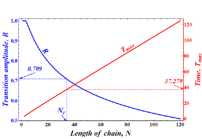
Figure 1: The maximum $R$ of the amplitude $R_{N}$ (solid decreasing line) and the appropriate time instant $\tau_{max}$ (solid increasing straight line) as functions of $N$. The plateau in the beginning of the decreasing line reflects the fact that $R(2)=R(3)=1$. The similar plateau appears in other figures below. The critical length $N_{c}=34$ is defined through the critical value $R_{c}=\frac{1}{\sqrt{2}}$ (see eq.51): $R(N_{c}+1)=0.704<R_{c}<R(N_{c})=0.709$. This is the maximal chain length allowing us to create the states with zero polarization and non-zero coherence intensity for any value of the inverse temperature $b$, see Sec.III.4.1. The value $R(N_{c})$ and the appropriate value $\tau_{max}(N_{c})=37.279$ are indicated in this figure.

III.2 Map of control-parameter space into creatable-parameter region

Apparently BZ_2015 , the spin dynamics in long chains compresses the creatable region so that the whole receiver’s state-space is divided into two parts: the creatable and unavailable regions. To visualize the creatable region, we represent the map

$$(\alpha,{b})\stackrel{{\scriptstyle(\ref{IJ},\ref{Jdef})}}{{\to}}(I,J)$$ (22)

(which is explicitly given by formulas (20) and (21)) in Fig.2 for the chains of different lengths $N$. As was mentioned in Sec.III.1, the whole state space of the one-qubit receiver can be created using the chain of two (or three) nodes, Fig.2a. If $N>3$, then the unavailable region appears, which is shown in Figs.2(b-d) (where the surrounding solid line is the boundary of the whole receiver’s state space (19)). In Fig.2, the dash-lines correspond to the constant values of the parameter $\alpha$, while the solid lines correspond to the constant values of the parameter ${b}$, therewith we use the following gridding throughout this paper:

$$\begin{array}[]{ll}\alpha=0.1n,\;\;n=0,1,\dots,10&{\mbox{dash-lines}},\cr{b}=0,\;0.1,\;\;0.5n,\;\;n=1,2,3,\dots&{\mbox{solid lines}}.\end{array}$$ (25)

We see that the solid lines nestle to the either line ${b}\to\infty$ or line ${b}=0$, which is most clearly shown in Fig.2c,d where only a few solid lines are well separated from the top and from the bottom of the bell-shaped creatable region. The shrinking to the line ${b}=0$ means that, increasing the chain length, we must decrease the temperature (or increase $b$) to create the valuable coherence intensity. As $N\to\infty$, the creatable region compresses to the right corner of the receiver’s state space, which, consequently, is the most reproducible area of the state space. On the contrary, the states in the left corners of the receiver’s state space become unavailable already in short chains, see Fig.2b.

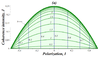
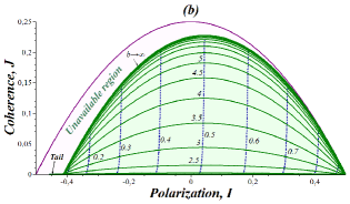
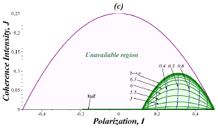
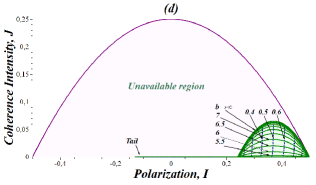
Figure 2: The creatable regions in the plane ($J,I$) for the chains of different lengths: (a) $N=2$, (b) $N=6$, (c) $N=60$ and (d) $N=120$. Here, as well as in all the figures below, we use gridding (25), therewith the solid- and dash-lines correspond to, respectively, $b=const$ and $\alpha=const$. The curves $b=const$ concentrate near the line $b\to\infty$. With an increase in $N$, their density near $b=0$ increases as well. The region of the receiver’s state space between the surrounding solid (violet) line (the parabola representing the boundary of the whole receiver state-space) and the bell-shaped creatable region is the unavailable region of the receiver state-space, which disappears for $N=2,3$. The well-formed tail of states with the vanishing coherence intensity is depicted in the cases $N=6$, 60 and 120 (figs. (b)-(d)) to the left of the bell-shaped region. In terms of the control parameters, this tail corresponds to the limit $\alpha\to 0$ (any $b$). The polarization of the tail’s end-point can be calculated by the formula $I=-\frac{R^{2}}{2}$, see eq.(47). With an increase in $N$, the creatable region shrinks to the point $(I,J)=(0,0)$, while the tail’s polarization becomes the interval $0\leq I\leq\frac{1}{2}$ covering the whole possible positive interval of the creatable polarization, see Sec.III.3.3.

The common feature of the creatable regions in Fig.2 is the tail (vanishing in chains of length $N=2,3$) of states with negligible coherence intensity situated to the left of the bell-shaped creatable region. This tail represents the ”classical” part of polarization, i.e., such polarization that causes negligible quantum effects described by the coherence intensity.

Notice, although the creatable region is mainly the one-to-one image of map (22), there is a small subregion which is the two-fold image of map (22). This feature is discussed in Sec.III.3.

III.3 One-to-one and two-to-one mapped creatable sub-regions

As mentioned in the Introduction, the whole creatable region is divided into the two subregions. One of them is the large subregion under the curve $b\to\infty$ in the plane $(I,J)$. This is the one-to-one image of map (22) (there is no intersections of solid lines inside of this region in Fig.2) with the control parameters inside of the following sub-domain:

$$\alpha^{br}(b)<\alpha\leq 1,\;\;0\leq b\leq\infty\;\;\;\;{\mbox{sub-domain of the one-to-one map (\ref{abIJ})}}.$$ (26)

Another subregion is the small area above the curve $b\to\infty$ (including the tail). This is the two-fold image of map (22) (in other words, the function $J(I)$ is a two-sheet function in this subregion) with the control parameters inside of the other sub-domain:

$$0\leq\alpha\leq\alpha^{br}(b),\;\;0\leq b\leq\infty\;\;\;\;{\mbox{sub-domain of the two-to-one map (\ref{abIJ})}},$$ (27)

Any point $(I,J)$ from this subregion can be created using two different pairs of the control parameters $(\alpha,b)$. This means, in particular, that two different values of temperature (parameter $b$) can create the same polarization and coherence intensity if the parameter $\alpha$ of the sender’s pure initial state properly depends on $b$. The boundary line $\alpha^{br}(b)$ in the plane of control parameters (separating the two above sub-domains (26) and (27)) is defined below in eq.(44).

III.3.1 One-to-one mapped subregion

First of all we observe that there is a curve covering the top of the bell-shaped creatable region, see Fig.2. It corresponds to the limit ${b}\to\infty$:

$$I_{\infty}=\frac{1}{2}\Big{(}(1-R^{2})-R^{2}\cos(\alpha\pi)\Big{)},$$ (28)

$$J_{\infty}=\frac{R^{2}}{4}\sin^{2}(\alpha\pi),\;\;0\leq\alpha\leq 1.$$ (29)

Formula (29) gives us the maximal value of $J$, $J^{max}_{\infty}$, at $\alpha=\frac{1}{2}$:

$$J^{max}_{\infty}=\frac{R^{2}}{4},$$ (30)

therewith, the appropriate polarization $I_{J_{max}}$ reads

$$I_{J_{max}}=\frac{1-R^{2}}{2}\geq 0.$$ (31)

In particular, for $N=2$ and 3, we have $R(2)=R(3)=1$ and $J^{max}_{\infty}=\frac{1}{4}$, $I_{J_{max}}=0$. Notice that $J_{\infty}$ vanishes at $\alpha=0,1$, therewith

$$I_{\infty}|_{\alpha=0}\equiv I_{c}=\frac{1}{2}-R^{2},\;\;I_{\infty}|_{\alpha=1}=\frac{1}{2}.$$ (32)

We must emphasize that the parametrically represented curve (28,29) is the upper boundary of the image of one-to-one map (22,26).

III.3.2 Creatable two-to-one mapped subregion

The two-to-one mapped subregion is a new feature of the remote state-creation process, which was not investigated before and thus deserves a special consideration. This subregion includes the tail to the left of the bell-shaped region and the close neighborhood of the left corner of this region in Fig.2. Since the scale of Fig.2 does not allow us to observe this subregion, we represent this subregion for the case $N=6$ using a suitable scale in Fig.3. Notice that the two-to-one mapped subregion disappears if $R=1$, i.e., $N=2,3$.

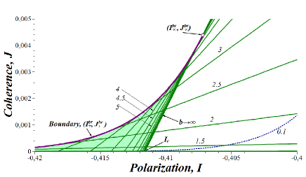
Figure 3: The left corner of the bell-shaped creatable region for the chain of $N=6$ nodes. The shaded area above the curve $b\to\infty$ (the boundary of the one-to-one mapped region) is covered by the two-to-one map (22,27), except for the upper boundary (one-to-one mapped), described by the points $(I^{br}_{+},J^{br}_{+})$ given in formulas (37) and (36) (the upper bold-solid (violet) line in the figure). The branch point $(I^{br}_{\infty},J^{br}_{\infty})=(-0.407,0.004)$ is the cross-point of this boundary line with the boundary of the one-to-one mapped region. The left point of the boundary line, corresponding to $b=0$, is $(-\frac{R^{2}}{2},0)\Big{|}_{N=6}=(-0.456,0)$ (this point is not shown in the graph). Therewith, the creatable area to the left of $I_{c}=-0.412$, $I<I_{c}$, corresponds to the two-sheet function $J(I)$ defined for all creatable values of $J$. Moreover, this subregion is creatable only at finite $b$ (non-zero temperature). We use gridding (25), so that only one dash-line $\alpha=0.1$ appears in this figure.

Now we derive the boundaries of the two-to-one mapped subregion. Apparently, map (22) is the one-to-one map at a point $(I,J)$ if $J|_{I=const}$ is a monotonic function of ${b}$ at this point. In the case of the two-to-one mapping, $J|_{I=const}$ as a function of $b$ loses its monotonic behavior and acquires the extremal point (a maximum). The appearance of such a maximum can be used as an indicator of the two-to-one mapping.

The upper boundary of this two-to-one mapped subregion can be parametrically described as follows. First, we solve eq.(20) for $\alpha$,

$$\cos(\alpha\pi)=\frac{1}{R^{2}}\Big{(}(1-R^{2})\tanh\frac{b}{2}-2I\Big{)},$$ (33)

and substitute $\alpha$ from eq.(33) into eq.(21) obtaining $J$ as a function of parameters $I$ and $b$, which now are considered as independent ones:

$$J(I,b)=\frac{\left(\tanh\frac{{b}}{2}\right)^{2(N-1)}}{4R^{2}}\left(R^{4}-\Big{(}2I-(1-R^{2})\tanh\frac{{b}}{2}\Big{)}^{2}\right).$$ (34)

Next, we calculate the partial derivative of $J$ with respect to $b$ and equate it to zero (we cancel positive factors and use the superscript ”$br$” to mark quantities associated with the two-sheet subregion):

$$4(I^{br})^{2}(N-1)-2I^{br}\tanh\frac{b^{br}}{2}(2N-1)(1-R^{2})+$$ (35)

$$\tanh^{2}\frac{b^{br}}{2}N(1-R^{2})^{2}-R^{2}(N-1)=0.$$

The lhs of eq.(35) is a quadratic expression in both $I^{br}$ and $\tanh\frac{b^{br}}{2}$. Let us solve it for the polarization $I^{br}$:

$$I^{br}_{\pm}=\frac{1}{4(N-1)}\left((2N-1)(1-R^{2})\tanh\frac{{b^{br}}}{2}\mp\sqrt{4(N-1)^{2}R^{4}+(1-R^{2})^{2}\tanh^{2}\frac{{b^{br}}}{2}}\right).$$ (36)

Substituting this polarization into eq.(34) we obtain the following expression for the coherence intensity:

$$J^{br}_{\pm}=\frac{(1-R^{2})R^{2}\left(\tanh\frac{{b^{br}}}{2}\right)^{2N-1}}{2\Big{(}(1-R^{2})\tanh\frac{{b^{br}}}{2}\pm\sqrt{4(N-1)^{2}R^{4}+(1-R^{2})^{2}\tanh^{2}\frac{{b^{br}}}{2}}\Big{)}}.$$ (37)

However, one can see that $J^{br}_{-}$ in formula (37) is negative, which is physically impossible. Thus, there is only one extremum point $(I^{br}_{+},J^{br}_{+})$ which is the maximum. The right hand sides of eqs.(36) and (37) are defined for all $N$ and $b^{br}$, i.e., any pair of values of these parameters uniquely defines the polarization $I^{br}_{+}$ such that the coherence intensity $J(I^{br}_{+},b)$ given in eq.(34) increases with $b$ till $b=b^{br}$, where $J$ takes its maximal value $J^{br}_{+}$, and then decreases either to its limit value $J(I^{br}_{+},\infty)>0$ or to zero. Thus, for a given $I^{br}_{+}$, the interval of coherence intensity $\max\Big{(}0,J(I^{br}_{+},\infty)\Big{)}\leq J<J^{br}_{+}$ is twice covered by map (22). Therewith,

$$0\leq J<J^{br}_{+},\;\;{\mbox{if}}\;\;I^{br}_{+}\leq I_{c},$$ (38)

where $I_{c}$ is defined in (32) as a polarization corresponding to $J_{\infty}=0$. In addition, the states with $I<I_{c}$ can be created only at finite $b$ (finite temperature) and can not exists as $b\to\infty$ (zero temperature). The polarization $I_{c}$ is marked in Fig.3 for $N=6$.

To estimate the size of the two-to-one mapped subregion, we calculate the maximal value of $J^{br}_{+}$ for a given $N$. It is clear that this maximum corresponds to ${b}\to\infty$:

$$J^{br}_{\infty}=\frac{(1-R^{2})R^{2}}{2\Big{(}(1-R^{2})+\sqrt{4(N-1)^{2}R^{4}+(1-R^{2})^{2}}\Big{)}}.$$ (39)

The appropriate expression for $I^{br}_{\infty}$ reads:

$$I^{br}_{\infty}=\frac{1}{4(N-1)}\left((2N-1)(1-R^{2})-\sqrt{4(N-1)^{2}R^{4}+(1-R^{2})^{2}}\right).$$ (40)

Thus, the upper boundary is parametrically defined by eqs.(36) and (37) (with the parameter $b^{br}$, $0\leq b^{br}<\infty$) over the interval

$$-\frac{R^{2}}{2}\leq I\leq I^{br}_{\infty}.$$ (41)

This boundary for the 6-node chain is represented in Fig.3 by the bold-solid (violet) line. Notice that $I^{br}_{\infty}$ changes its negative sign to the positive one in passing from $N=33$ to $N=N_{c}=34$. The point $(J^{br}_{\infty},I^{br}_{\infty})$ can be referred to as a branch point because, passing through this point, the function $J(I,b)$ becomes a two-sheet function of $b$. This point is marked in Fig.3 ($N=6$). Notice also that, by construction, the upper boundary itself is ones covered by the control parameters.

Regarding the right boundary of the two-to-one mapped subregion (see the right boundary of the shaded area in Fig.3), it is described by the part of the curve $b\to\infty$ (28,29) over the interval

$$I_{c}\leq I\leq I^{br}_{\infty}.$$ (42)

This boundary is an image of the boundary $\alpha^{br}(b)$ in the control parameter plane (separating the preimages of the one-to-one and two-to-one mapped subregion ), which was used in eqs.(26,27). This boundary consists of the intersection points of the curves $b=const$ with the curve $b\to\infty$, i.e, $\alpha^{br}$ satisfies the following system

$$I(\alpha^{br},b)=I(\tilde{\alpha},\infty),$$ (43)

$$J(\alpha^{br},b)=J(\tilde{\alpha},\infty)$$

for some $\tilde{\alpha}$. Here, $I(\alpha,b)$ and $J(\alpha,b)$ are given in eqs.(20) and (21). Solving this system we obtain

$$\cos(\alpha^{br}\pi) = \frac{(1-R^{2})(1-\tanh\frac{b}{2})\tanh^{2}\frac{b}{2}-\sqrt{D}}{R^{2}\left(\left(\tanh\frac{b}{2}\right)^{2N}-\tanh^{2}\frac{b}{2}\right)},$$ (44)

$$D = R^{4}\Big{(}\tanh^{4}\frac{b}{2}+\tanh^{4N}\frac{b}{2}\Big{)}+$$

$$\left(\tanh\frac{b}{2}\right)^{2(N+1)}\Big{(}\Big{(}1-\tanh\frac{b}{2}\Big{)}^{2}(1-2R^{2})+R^{4}(\tanh^{2}\frac{b}{2}-2\tanh\frac{b}{2}-1)\Big{)}.$$

III.3.3 Interval of creatable polarization and tail with vanishing coherence intensity

The interval of creatable polarization at a given $b$ is defined by the boundary values of the parameter $\alpha$. Thus, at $\alpha=0$ and $\alpha=1$, we obtain, respectively, the lower and upper boundaries of polarization as functions of $b$ from eq.(20):

$$I_{low}(b)=\frac{1}{2}\left((1-R^{2})\tanh\frac{b}{2}-R^{2}\right)$$ (45)

$$\ I_{up}(b)=\frac{1}{2}\left((1-R^{2})\tanh\frac{b}{2}+R^{2}\right).$$ (46)

Therewith the minimal value of $I_{low}$ corresponds to $b=0$, while the maximal value of $I_{up}$ corresponds to $b\to\infty$; thus the maximal variation interval of $I$ is the following one:

$$-\frac{R^{2}}{2}=I_{low}(0)\leq I\leq I_{up}(\infty)=\frac{1}{2}$$ (47)

In the case $N=2,3$, we have $R\equiv 1$, so that inequality (47) reaches the boundary of the receiver’s state space: $|I|\leq\frac{1}{2}$.

Considering the polarization at the fixed temperature, $I_{low}(b)\leq I\leq I_{up}(b)$, we point out the two following limit intervals:

$$\frac{1}{2}(1-2R^{2})\leq I\leq\frac{1}{2},\;\;\;b\to\infty$$ (48)

$$-\frac{R^{2}}{2}\leq I\leq\frac{R^{2}}{2},\;\;\;b=0.$$ (49)

As $N\to\infty$ (consequently, $R\to 0$), each of the above intervals shrinks into a point, and formulas (20) and (21) show that the creatable polarization is completely defined by the temperature (the parameter $\alpha$ of the sender’s pure initial state disappears in this limit): $I\to\frac{1}{2}\tanh\frac{b}{2}$, and $J\to 0$. Thus, the variation interval of the polarization tends to $0\leq I\leq\frac{1}{2}$ covering the whole positive interval of the creatable polarization, while the coherence intensity tends to zero for any temperature. This is a principal difference between the polarization and the coherence intensity. Notice that the above limit interval coincides with the limit $N\to\infty$ of the tail of polarization (see Fig.2), which covers the interval $-\frac{R^{2}}{2}\leq I\leq I^{br}_{\infty}$ in the case of finite $N$.

III.4 Mutual relations between creatable polarization and coherence intensity

Although the parameters of the creatable region discussed in Sec.III.3 can be referred to as characteristics of the creatable region, they describe mainly the boundary of this region. Now we introduce some characteristics reflecting mutual relation between creatable polarization and coherence intensity inside of the creatable region.

III.4.1 States with zero polarization

In this subsection, we consider the case $I=0$, when the coherence intensity (which is associated with quantum effects) is created without polarization (classical effect). In this case, eq.(14) yields $\rho_{11}=\frac{1}{2}$, and eq.(20) results in the following relation between the control parameters $\alpha$ and ${b}$ (we use the superscript ”$(0)$” to differ the quantities of this subsection from those of the general position):

$$\cos(\alpha^{(0)}\pi)=\frac{1-R^{2}}{R^{2}}\tanh\frac{{b}^{(0)}}{2}>0.$$ (50)

This relation holds for any $b^{(0)}$ if

$$\frac{1-R^{2}}{R^{2}}\leq 1,\;\;\Leftrightarrow\;\;R^{2}\geq\frac{1}{2}\stackrel{{\scriptstyle{\mbox{def}}}}{{=}}R_{c}^{2}.$$ (51)

The direct calculation shows (see also Fig.1) that

$$R(35)=0.704<R_{c}<R(34)=0.709.$$ (52)

Consequently, inequalities (51) hold if

$$N\leq N_{c}=34.$$ (53)

Otherwise, if $N>N_{c}$, then eq.(50) yields the following constraint for $b^{(0)}$:

$$\tanh\frac{{b}^{(0)}}{2}\leq\frac{R^{2}}{1-R^{2}}.$$ (54)

Substituting eq.(50) into eq.(21) we obtain

$$J^{(0)}=\frac{\Big{(}\tanh\frac{{b}^{(0)}}{2}\Big{)}^{2(N-1)}}{4R^{2}}\left(R^{4}-(1-R^{2})^{2}\tanh^{2}\frac{{b}^{(0)}}{2}\right), \;\;\forall\;b^{(0)},\;\;N\leq N_{c}\;\;{\mbox{or}}$$

$${\mbox{for $b^{(0)}$ satisfying (\ref{constrIJ})}},\;\;N>N_{c}.$$

Considering $J^{(0)}$ in (III.4.1) as a function of ${b}^{(0)}$, we find its maximum at

$$\tanh\frac{{b}^{(0)}_{max}}{2}=\left\{\begin{array}[]{ll}1,&N<N_{c}\cr\frac{R^{2}}{1-R^{2}}\sqrt{\frac{N-1}{N}},&N\geq N_{c}\cr\end{array}\right..$$ (58)

In deriving eq.(58), we take into account that $\left|\tanh\frac{{b}^{(0)}_{max}}{2}\right|\leq 1$ and

$$\left.\frac{R^{2}}{1-R^{2}}\sqrt{\frac{N-1}{N}}\right|_{N=34}=0.993<1<\left.\frac{R^{2}}{1-R^{2}}\sqrt{\frac{N-1}{N}}\right|_{N=33}=1.021.$$ (59)

Thus, substituting eq.(58) into eq.(III.4.1), we obtain

$$J^{(0)}_{max}=\left\{\begin{array}[]{cc}\frac{2R^{2}-1}{4R^{2}},&N<N_{c}\cr\frac{(N-1)^{N-1}R^{2(2N-1)}}{4N^{N}(1-R^{2})^{2(N-1)}},&N\geq N_{c}\cr\end{array}\right..$$ (62)

In addition, substituting eq.(58) into eq.(50), we have

$$\cos(\alpha^{(0)}_{max}\pi)=\left\{\begin{array}[]{cc}\frac{1-R^{2}}{R^{2}},&N<N_{c}=34\cr\sqrt{\frac{N-1}{N}},&N\geq N_{c}\end{array}\right..$$ (65)

The dependence of $J^{(0)}_{max}$, ${b}^{(0)}_{max}$ and $\alpha^{(0)}_{max}$ on $N$ is depicted in Fig.4. All graphs have breakpoints at $N=N_{c}$.

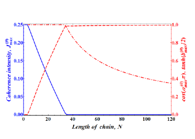
Figure 4: The characteristics of the states with zero polarization. The creatable coherence intensity $J^{(0)}_{max}$ (solid line) and the appropriate control parameters (in the form of $\tanh\frac{{b}^{(0)}_{max}}{2}$ (dash-dot-line) and $\cos(\alpha^{(0)}_{max}\pi)$ (dash-line)) are given as functions of $N$. All graphs have breakpoints at $N=N_{c}=34$. For $N>N_{c}$, the coherence intensity vanishes very rapidly with an increase in $N$, see (66).

Fig.4 demonstrates that, for $N\geq N_{c}$, the parameter $J^{(0)}_{max}$ vanishes very rapidly with increase in $N$. Thus,

$$J^{(0)}_{max}|_{N=34}=2.367\;\;10^{-3},\;\;J^{(0)}_{max}|_{N=40}=1.782\;\;10^{-8},\;\;J^{(0)}_{max}|_{N=50}=3.012\;\;10^{-18}.$$ (66)

This means that the significant value of the coherence intensity can not be created without the supplementing polarization in long chains. The minimal polarization needed for creation of the measurable coherence intensity is studied in the next subsection.

III.4.2 States with detectable coherence intensity

Since the coherence intensity can not be created without the polarization in long chains, important characteristics of the state creation are such minimal $I^{(1)}_{-}$ and maximal $I^{(1)}_{+}$ values of the polarization $I$ (at a fixed ${b}$) that the creatable coherence intensity $J$ is valuable (i.e., exceeds some conventional value $J_{min}$) inside of the interval $I^{(1)}_{-}\leq I\leq I^{(1)}_{+}$.

For a given ${b}$, the intensity $J$ reaches its prescribed (registrable) value $J_{min}$ for the two values of $\alpha$:

$$\cos(\alpha^{(1)}_{\pm}\pi)=\mp\sqrt{1-\frac{4J_{min}}{R^{2}}\left(\tanh\frac{{b}}{2}\right)^{2(1-N)}}.$$ (67)

Apparently, the expression under the square root must be non-negative, which holds for ${b}\geq{b}^{(1)}$, where the critical value $b^{(1)}$ corresponds to zero under the square root in expression (67):

$$\tanh\frac{{b}^{(1)}}{2}=\left(\frac{4J_{min}}{R^{2}}\right)^{\frac{1}{2(N-1)}}.$$ (68)

Next, substituting eq.(67) into (20), we eliminate dependence on $\alpha$ obtaining

$$I^{(1)}_{\pm}=\frac{1}{2}\left((1-R^{2})\tanh\frac{{b}}{2}\pm R\sqrt{R^{2}-4J_{min}\left(\tanh\frac{{b}}{2}\right)^{2(1-N)}}\right)$$ (69)

The maximal $I^{(1)}_{+}$ and minimal $I^{(1)}_{-}$ values correspond to, respectively, the upper and lower signs in formula (69) (these parameters are related to, respectively, the right and left corners of the bell-shaped region). Apparently, at $b=b^{(1)}$, the minimal and maximal values of coherence intensity coincide: $I^{(1)}_{-}=I^{(1)}_{+}=I^{(1)}_{c}$, where

$$I^{(1)}_{c}=\frac{(1-R^{2})}{2}\left(\frac{4J_{min}}{R^{2}}\right)^{\frac{1}{2(N-1)}},$$ (70)

and the appropriate parameter $\alpha$ equals $\alpha^{(1)}_{c}=\frac{1}{2}$, which follows from eq.(67) at $b=b^{(1)}$. Parameters $I^{(1)}_{-}$, $I^{(1)}_{+}$ together with the associated values of the control parameters $\alpha^{(1)}_{-}$, $\alpha^{(1)}_{+}$ as functions of the chain length $N$ for different values of $b$ in the list

$${b}=b^{(1)}(10n),\;\;n=1,2,\dots,$$ (71)

and $J_{min}=0.01$ are depicted in Fig.5. The critical intensity $I^{(1)}_{c}$ and the critical parameter $\alpha^{(1)}_{c}$ are shown, respectively, in Figs.5a and 5b by the dash-lines.

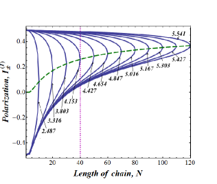
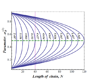
Figure 5: The creatable states with the low coherence intensity. (a) The polarization $I^{(1)}_{-}$ (curves below the dash-line $I^{(1)}_{c}$), $I^{(1)}_{+}$ (curves above the dash-line $I^{(1)}_{c}$). (b) The associated values of the control parameter $\alpha$, $\alpha^{(1)}_{-}$ (curves below the dash-line $\alpha^{(1)}_{c}=\frac{1}{2}$), $\alpha^{(1)}_{+}$ (curves above the dash-line $\alpha^{(1)}_{c}$). All parameters are given as functions of the chain length $N$ for $J_{min}=0.01$. Each curve corresponds to the particular $b$ from set (71), where $n$ increases from the left to the right lines in this figure, for instance, $b^{(1)}(10)=2.487$.

Parameters ${b}^{(1)}$ and $I^{(1)}_{c}$ can be considered as the minimal required value of $b$ (or the maximal allowed temperature) and the associated minimal value of the polarization required for creating the conventional value $J_{min}$ of the coherence intensity.

The interpretation of Fig.5 is evident. The vertical line corresponding to the given chain length $N$ (see the vertical dot-lines in Figs.5a and 5b for $N=40$) crosses each line $b\geq b^{(1)}(N)$ at the two points: $I^{(1)}_{+}(b)$ and $I^{(1)}_{-}(b)$ in Fig.5a and $\alpha^{(1)}_{+}(b)$ and $\alpha^{(1)}_{-}(b)$ in Fig.5b (these points are not marked in Fig.5). These cross-points give the intervals of the polarization and the appropriate intervals of the parameter $\alpha$ allowing us to create the measurable coherence intensity $J\geq J_{min}$.

III.5 Integral characteristics: fidelity of remote state creation

III.5.1 Fidelity of remote state creation

As characteristics of the remote state creation, we propose the following integral characteristics, which we refer to as the fidelity of the remote state creation $F(N)$ (by analogy with the similar characteristics of the state transfer Bose ) and define by the following general formula:

$$F(N)=\frac{S_{creatable}}{S_{receiver}}$$ (72)

where $S_{creatable}$ is the area of the creatable region and $S_{receiver}$ is the area of the receiver’s state space. In turn, $S_{creatable}$ can be splitt into two parts: the area of the one-to-one mapped creatable sub-region $S_{1-to-1}$ and the area of the two-to-one mapped creatable sub-region $S_{2-fold}$, so that

$$F(N)=F_{1-to-1}(N)+F_{2-fold}(N),$$ (73)

$$F_{1-to-1}(N)=\frac{S_{1-to-1}}{S_{receiver}},\;\;\;F_{2-fold}(N)=\frac{S_{2-fold}}{S_{receiver}}.$$

In our case, $S_{receiver}$ can be calculated analytically using the boundary of region (19) $J=\frac{1}{4}-I^{2}$ and integrating it over the interval $-\frac{1}{2}\leq I\leq\frac{1}{2}$:

$$S_{receiver}=\frac{1}{6}.$$ (74)

The function $S_{1-to-1}$ can be also calculated analytically eliminating $\alpha$ from eq.(29) by means of eq.(28) and integrating the obtained coherence intensity $J_{\infty}$ as a function of polarization $I_{\infty}$,

$$J_{\infty}=\frac{1}{4R^{2}}(1-2I_{\infty})(2I_{\infty}+2R^{2}-1),$$ (75)

over the interval $I_{c}\leq I_{\infty}\leq\frac{1}{2}$:

$$S_{1-to-1}=\frac{R^{4}}{6}.$$ (76)

Finally, the function $S_{2-fold}(N)$ can be calculated numerically using the formulas (36) and (37) for the upper boundary of this region (over interval (41)) and (75) for the right boundary (over interval (42)):

$$S_{2-fold}=\int\limits_{-\frac{R^{2}}{2}}^{I^{br}_{\infty}}dI\;J^{br}_{+}(I)-\frac{1}{4R^{2}}\int\limits_{I_{c}}^{I^{br}_{\infty}}dI\;(1-2I)(2I+2R^{2}-1),$$ (77)

where $I_{c}$ and $I^{br}_{\infty}$ are defined in eqs.(32) and (40) respectively. Expression for $J^{br}_{+}(I)$ in integral (77) follows from eq.(37) after eliminating $\tanh\frac{b^{br}}{2}$ by means of eq.(36). The fidelities $F_{1-to-1}$ and $F_{2-fold}$ as functions of $N$ are depicted in Fig.6.

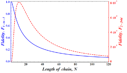
Figure 6: The creation fidelities of the one-to-one (bold line) and the two-to-one (dash-line) mapped states are shown as functions of the chain length $N$. The fidelity of the two-to-one mapped region is much less than that of the one-to-one mapped region and has the maximum at $N=12$.

This figure shows the smallness of the two-to-one mapped sub-region in comparison with the one-to-one mapped one in our model. We can also see the maximum of the fidelity $F_{2-fold}(N)$ at $N=12$.

III.5.2 Average creatable polarization and coherence intensity as functions of temperature

The interesting characteristics are the polarization and the coherence intensity averaged over the initial pure state of the sender:

$$\bar{I}(b) = \int\limits_{0}^{1}I(\alpha,b)d\alpha=\frac{1-R^{2}}{2}\tanh\frac{b}{2},$$ (78)

$$\bar{J}(b) = \int\limits_{0}^{1}J(\alpha,b)d\alpha=\frac{R^{2}}{8}\left(\tanh\frac{b}{2}\right)^{2(N-1)}.$$ (79)

where $I$ and $J$ are defined in eqs.(20) and (21), respectively. Equations (78) and (79) show that both the mean polarization and the mean coherence intensity increase with $b$. Therewith, the mean polarization increases also with $N$, while the mean coherence intensity decreases with $N$. The families of curves $\bar{I}(b)$ and $\bar{J}(b)$ are represented in Fig.7 for different $N$.

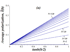
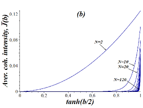
Figure 7: The polarization (a) and the coherence intensities (b) averaged over the control parameter $\alpha$ are shown as functions of the inverse temperature $b$ for chains of different lengths $N$, $N=2,10,20,\dots,120$.

IV Parametrization of receiver’s density matrix in terms of independent eigenvalue-eigenvector parameters

Although the physically motivated parametrization considered in Sec.III allows us to give a comprehensive description of the creatable region together with its physical interpretation in terms of polarization and coherence intensity, we consider another parametrization in terms of the receiver’s eigenvalues and eigenvectors. The motivation for this parametrization is the comparison of our model of remote state creation with that described in BZ_2015 , where the homogeneous chain with the pure initial state of the two-qubit sender and ground initial state of the rest system was considered, therewith the receiver was a one-qubit subsystem as well.

Thus, we represent state (7) of the receiver in the following factorized form:

$$\rho^{N}=U^{N}\Lambda^{B}(U^{N})^{+},$$ (80)

where $\Lambda^{N}$ is the diagonal matrix of eigenvalues and $U^{N}$ is the matrix of eigenvectors, which read as follows in our case:

$$\Lambda^{N}={\mbox{diag}}(\lambda,1-\lambda),$$ (81)

$$U^{N}=\left(\begin{array}[]{cc}\cos\frac{\beta_{1}\pi}{2}&-e^{-2i\beta_{2}\pi}\sin\frac{\beta_{1}\pi}{2}\cr e^{2i\beta_{2}\pi}\sin\frac{\beta_{1}\pi}{2}&\cos\frac{\beta_{1}\pi}{2}.\end{array}\right)$$ (84)

with $\lambda$ and $\beta_{i}$ ($i=1,2$) varying inside of the intervals

$$\frac{1}{2}\leq\lambda\leq 1,$$ (85)

$$0\leq\beta_{i}\leq 1,\;\;i=1,2.$$ (86)

Comparing eq.(80) with eq.(7) we establish the relation between the control parameters $(\alpha,{b},\phi)$ and the creatable parameters $(\lambda,\beta_{1},\beta_{2})$:

$$\lambda=\frac{1}{2}\left(1+\sqrt{(2\rho^{N}_{11}-1)^{2}+4|\rho_{12}|^{2}}\right)=$$

$$\frac{1}{2}\left(1+\sqrt{1+\Delta_{0}}\Big{|}R^{2}\cos(\alpha\pi)-(1-R^{2})\tanh\frac{{b}}{2}\Big{|}\right),$$

$$\cos(\beta_{1}\pi)=\frac{2\rho^{N}_{11}-1}{2\lambda-1}=$$

$$-\frac{1}{\sqrt{1+\Delta_{0}}}{\mbox{sign}}(R^{2}\cos(\alpha\pi)-(1-R^{2})\tanh\frac{{b}}{2})$$

$$\beta_{2}=\Phi_{N}(\tau)+\phi+\frac{1}{2}(N-1),$$ (89)

where

$$\Delta_{0}=\frac{R^{2}\sin^{2}(\alpha\pi)\Big{(}\tanh\frac{{b}}{2}\Big{)}^{2(N-1)}}{(R^{2}\cos(\alpha\pi)-(1-R^{2})\tanh\frac{{b}}{2})^{2}}$$ (90)

Intervals (85) and (86) cover the whole state-space of the receiver. We see that any parameter $\beta_{2}$ can be created at the fixed time instant $\tau$ using the control parameter $\phi$: $\phi=\beta_{2}(\tau)-\Phi_{N}(\tau)-\frac{(N-1)}{2}$. For this reason, similar to Sec.III, we consider density matrix (13) instead of (7) and thus, studying the map (control parameters) $\to$ (creatable parameters), we turn to the reduced map

$$(\alpha,b)\stackrel{{\scriptstyle(\ref{lam},\ref{bet})}}{{\to}}(\lambda,\beta_{1})$$ (91)

instead of the complete map $(\alpha,b,\phi)\stackrel{{\scriptstyle(\ref{lam},\ref{bet},\ref{bet2})}}{{\to}}(\lambda,\beta_{1},\beta_{2})$.

Notice that two independent pairs of the control parameters $\{I,J\}$ and $\{\lambda,\beta_{1}\}$ are related by the following one-to-one map:

$$\begin{array}[]{l}\lambda=\frac{1}{2}+\sqrt{I^{2}+J}\cr\cos\beta_{1}\pi=\frac{I}{\sqrt{I^{2}+J}}\end{array}\;\;\Leftrightarrow\;\;\begin{array}[]{l}I=\Big{(}\lambda-\frac{1}{2}\Big{)}\cos(\beta_{1}\pi)\cr\sqrt{J}=\Big{(}\lambda-\frac{1}{2}\Big{)}\sin(\beta_{1}\pi)\end{array}.$$ (96)

Formulas in (96) suggest us to combine all these parameters in single relation introducing the following complex function $\Xi$:

$$\Xi\equiv I+i\sqrt{J}=\Big{(}\lambda-\frac{1}{2}\Big{)}e^{i\beta_{1}\pi}.$$ (97)

IV.1 Creatable regions for homogeneous chains of different lengths

Here we describe the creatable regions in chains of different lengths. The maximal region corresponds to $N=2$ or $3$, as shown in Fig.8a.

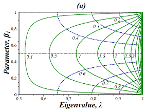
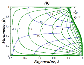
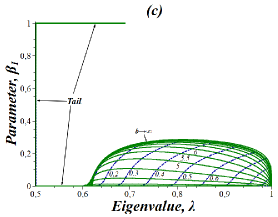
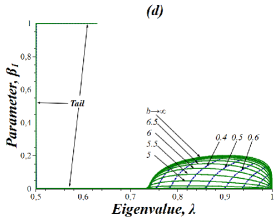
Figure 8: The creatable regions in the space of the creatable parameters $\lambda$ and $\beta_{1}$ for (a) $N=2$, (b) $N=6$, (c) $N=60$, and (d) $N=120$. General behavior of the curves $b=const$ (solid lines) and $\alpha=const$ (dash-lines) is similar to that of curves in Fig.2. In particular, the curves $b=const$ concentrate near the curve $b\to\infty$. With an increase in $N$, their density near $b=0$ increases as well. For $N=2$, the line $b\to\infty$ coincides with the right coordinate line of the parameter $\beta_{1}$. The tail of the states with vanishing $I$ is well formed in the cases $N=6$, 60 and 120 (shown in figs. (b)-(d)). This tail corresponds to $\alpha\to 0$ (any $b$), similar to Fig.2. The unavailable region appears if $N>3$.

The common feature of the creatable regions in Fig.8 is the tail of states with $\beta_{1}\to 0,1$ appearing in chains of the length $N>3$, similar to the case of physical parametrization shown in Fig.2. But now the tail is ”crooked” for large $N$, as shown in Fig.8c,d.

Formulas (96) allow us to rewrite all characteristics of the creatable region found in Sec.III in terms of the parameters $\lambda$ and $\beta_{1}$. In particular, using formulas (96), we conclude that

$$\beta_{1}\to 0\;\;\Leftrightarrow\;\;I>0,\;J\to 0,$$ (98)

$$\beta_{1}\to 1\;\;\Leftrightarrow\;\;I<0,\;J\to 0.$$

Therewith there is a particular case $I=0$ yielding

$$\beta_{1}^{cr}=\frac{1}{2}\;\;\Leftrightarrow\;\;I=0.$$ (99)

Now, eq.(IV) with $\beta_{1}=\frac{1}{2}$ yields eq.(50), while eq.(IV) results in

$$\lambda^{(0)}=\frac{1}{2}\left(1+\sqrt{R^{4}-(1-R^{2})^{2}\tanh^{2}\frac{{b^{(0)}}}{2}}\Big{(}\tanh\frac{{b^{(0)}}}{2}\Big{)}^{N-1}\right).$$ (100)

Eq.(50) holds for all $b$ if condition (51) is satisfied, which leads to the critical value $N_{c}=34$ obtained in Sec.III.4.1 and in Ref.BZ_2015 . Thus, inequality (54) holds for all $b$ if $N\leq N^{c}$. For $N>N^{c}$, condition (54) is satisfied if

$$b\leq{b^{(0)}}=2\;{\mbox{atanh}}\frac{R^{2}}{1-R^{2}}.$$ (101)

This means that the curves ${b}=const>{b^{(0)}}$ on the graphs do not reach the upper boundary $\beta_{1}=1$, while the other curves (${b}=const\leq{b^{(0)}}$) reach it. Notice also that the state with $\lambda=\frac{1}{2}$ assumes arbitrary $\beta_{1}$. Thus, the whole vertical line $\lambda=\frac{1}{2}$ in Figs.8 represents the same state.

Similarly to Fig.2, the whole creatable region is divided into two parts: the image of one-to-one map (91,26) (the main part of the creatable region) and the image of two-to-one map (91,27), which is the tail together with the close neighborhood of the corner where this tail attaches to the main part of the creatable region. These two subregions are separated one from another by the curve ${b}\to\infty$ (see Fig.8):

$$\lambda|_{{b}\to\infty}=\frac{1}{2}\left(1+\sqrt{(R^{2}(\cos(\alpha\pi)+1)-1)^{2}+R^{2}\sin^{2}(\alpha\pi)}\right),$$ (102)

$$\cos(\beta_{1}\pi|)|_{{b}\to\infty}=-\frac{R^{2}(\cos(\alpha\pi)+1)-1}{\sqrt{(R^{2}(\cos(\alpha\pi)+1)-1)^{2}+R^{2}\sin^{2}(\alpha\pi)}}.$$ (103)

With an increase in $N$, the creatable region vanishes. Here we shall emphasize the important difference between the model of Ref.BZ_2015 and our one. Unlike that model, any eigenvalue can be simply created in our case as the parameter associated with the classical limit. On the contrary, the parameter $\beta_{1}$, characterizing the eigenvector, has restrictions for its creatable values in both models.

V Conclusion

We consider the remote creation of the polarization and the intensity of the first-order coherence in a spin-1/2 chain with the physically motivated initial condition: the pure state of the one-qubit sender and the thermodynamic equilibrium state of the rest nodes. Therewith, the polarization is basically responsible for the classical effects (the diagonal part of the density matrix) while the coherence intensity is responsible for the quantum effects (the non-diagonal part of the density matrix). Using this physical parametrization, we obtain the following properties and characteristics of the creatable region of the receiver state-space in our model.

1. At the fixed temperature (parameter $b$), we can use the parameter $\alpha$ of the sender’s initial state as the control parameter varying the values of the polarization and the coherence intensity (i.e, the parameter $\alpha$ moves the state $(I,J)$ along the chosen solid curve in Fig.2)). Thus, the temperature is not the only parameter responsible for the remotely creatable polarization and coherence intensity (Sec.III.2).

2. The creatable region is divided into two subregions covered by, respectively, one-to-one map (22,26) and two-to-one map (22,27), therewith the biggest subregion is created by the one-to-one map, which is, essentially, the bell-shaped regions in Fig.2. The boundaries of these subregions are described, see Secs.III.3.1 and III.3.2.

3. Any state $(I,J)$ from the two-to-one mapped subregion (except the upper boundary ($I^{br}_{+},J^{br}_{+}$) given in (36,37)) can be created using the two different pairs of the control parameters $(\alpha,b)$. In particular, this can be achieved fixing $\alpha$ (i.e., the pure state of the one-node sender) and varying the temperature or vise-versa (Sec.III.3.2).

4. The tail of states with vanishing coherence intensity and large polarization is well formed to the left of the bell-shaped region. This tail is referred to the two-to-one mapped subregion, see Sec.III.3.3.

5. The states with zero polarization $I$ and large coherence intensity $J$ are described in Sec.III.4.1. Such states are creatable only in short chains. With an increase in $N$, the significant value of the coherence intensity can be created only together with the large polarization.

6. On the contrary, the large polarization can be created without the coherence intensity in the long chains, which justifies the classical origin of the polarization, see Sec.III.4.2. Moreover, as $N\to\infty$, the creatable intensity shrinks to the interval $0\leq I\leq\frac{1}{2}$.

7. For a given $N$ and $b>b^{(1)}$, the measurable value of the coherence intensity $J\geq J_{min}$ can be achieved only for $\alpha$ chosen inside of the interval $\alpha^{(1)}_{-}\leq\alpha\leq\alpha^{(1)}_{+}$ (and consequently, the value of creatable polarization $I$ is inside of the interval $I^{(1)}_{-}\leq I\leq I^{(1)}_{+}$), Sec.III.4.2.

8. We introduce the integral characteristics of the remotely created region (as well as of the both one-to-one and two-to-one mapped subregions) as the ratio of the area of the creatable (sub)region to the area of the whole receiver state-space, see Sec.III.5. By analogy with the pure state transfer, we refer to this characteristics as the state-creation fidelity. The polarization and coherence intensity averaged over the sender’s initial state are also found as functions of the inverse temperature $b$ and chain length $N$.

9. To simplify the comparison of our model with the state creation model proposed in BZ_2015 , we also consider the alternative parametrization in terms of the eigenvalue and eigenvectors of the receiver state in Sec.IV. A principal distinctions of our model is the possibility to transfer any eigenvalue over the homogeneous spin chain of any length $N$, while this length is restricted by the critical value $N_{c}=34$ in BZ_2015 .

Thus we represent the analysis of the creatable polarization and coherence intensity, which are uniquely related with the state of one-qubit receiver. In turn, the state of multi-qubit receiver can be (partially) characterized by the intensities of multiple quantum coherences, for which the detection methods are well developed BMGP ; F .

Now we underline several problems of interest prompted by our results.

First of all, the study of the possibility to use a local tool on the receiver site with the purpose to increase the creatable space of the receiver (i.e., fidelity). Since any eigenvalue can be transfered, then, in principle, this problem can be solved using the local unitary transformation on the receiver side. However, the local transformations independent on the control parameters (the parameters $\alpha$ and $b$ in our case) would be of general interest. The way realizing such the local transformations is not evident.

Next, we must keep in mind the problem of remote control of quantum operations based on mixed states. In this regards, the two-to-one mapped subregion might be useful. In particular, an ambiguity of the control parameters creating the given state would be of possible interest in quantum cryptography GRTZ , which is another applicability direction of quantum information devises HBB ; SCCS .

In addition, one should remember that the parameter $b$ (the inverse temperature) is one of the control parameters, which is not a sender’s local parameter, but the characteristics of the chain as a whole. Thus, we must be able to provide the constant temperature in the whole sample containing our spin chain.

Notice also that the temperature is a global parameter of the whole chain. This means that the remote state creation in our model partially loses its control exclusively by the local parameters of the sender. However, since the chain’s established temperature is a known parameter on the receiver’s site, we do not need to transfer this parameter through any classical communication channel.

This work is partially supported by the Russian Foundation for Basic Research, grants No.15-07-07928 and No.16-03-00056, and by the Program of RAS ”Element base of quantum computers” (grant No.0089-2015-0220).

VI Appendix A: Amplitude $R_{N}(\tau)$ as a characteristics of transmission line

The nearest neighbor Hamiltonian (4) can be diagonalized using the Jordan-Wigner transformation method JW ; CG :

$$H=\sum_{k}\varepsilon_{k}\beta_{k}^{+}\beta_{k},\;\;\varepsilon_{k}=\cos(k),\;\;\displaystyle k=\frac{\pi n}{N+1},\;\;\;n=1,2,\dots,N,$$ (104)

where $\beta_{j}$ are the fermion operators, introduced in terms of the other fermion operators $c_{j}$ using the Fourier transformation

$$\beta_{k}=\sum_{j=1}^{N}g_{k}(j)c_{j},$$ (105)

where the fermion operators $c_{j}$ read

$$c_{j}=(-2)^{j-1}I_{1z}I_{2z}\dots I_{(j-1)z}I^{-}_{j}.$$ (106)

Here

$$g_{k}(j)=\left(\frac{2}{N+1}\right)^{1/2}\sin(kj).$$ (107)

The projection operators $I_{jz}$ can be represented as

$$I_{jz}=c^{+}_{j}c_{j}-\frac{1}{2},\;\;\forall\;j.$$ (108)

Before proceed to the derivation of the density matrix evolution, we rewrite initial density matrix (2) in the following operator form

$$\rho_{0}=\frac{1}{Z}(\frac{1}{2}E+(|a_{0}|^{2}-|a_{1}|^{2})I_{z1}+a_{0}a_{1}^{*}I^{+}_{1}+a_{1}a_{0}^{*}I^{-}_{1})e^{-{b}I_{z1}}e^{{b}I_{z}}=$$ (109)

$$\frac{1}{Z}(A_{1}E+A_{2}I_{z1}+A_{3}I^{+}_{1}+A_{4}I^{-}_{1})e^{{b}I_{z}},$$

where $E$ is the $2\times 2$ unit operator,

$$Z=\left(2\cosh\frac{{b}}{2}\right)^{N-1},\;\;I_{z}=\sum_{i=1}^{N}I_{zi},$$ (110)

$$A_{1}=\frac{1}{2}e^{-\frac{{b}}{2}}+|a_{1}|^{2}\sinh\frac{{b}}{2},\;\;\;A_{2}=e^{-\frac{{b}}{2}}-2|a_{1}|^{2}\cosh\frac{{b}}{2},$$

$$A_{3}=a_{0}a_{1}^{*}e^{\frac{{b}}{2}},\;\;\;A_{4}=a_{0}^{*}a_{1}e^{-\frac{{b}}{2}}.$$

Since $[H,I_{z}]=0$, the evolution of the density matrix can be written as

$$\rho(\tau)=\frac{1}{Z}\sum_{i=1}^{4}{r_{i}(\tau)}e^{{b}I_{z}},$$ (111)

with

$$r_{1}(\tau)=A_{1},\;\;$$ (112)

$$r_{2}(\tau)=A_{2}\left(-\frac{1}{2}+\sum_{k,k^{\prime}=1}^{N}e^{-i\tau(\varepsilon_{k}-\varepsilon_{k^{\prime}})}g_{1k}g_{1k^{\prime}}\beta^{+}_{k}\beta_{k^{\prime}}\right),$$

$$r_{3}(\tau)=A_{3}\sum_{k=1}^{N}e^{-i\tau\varepsilon_{k}}g_{1k}\beta^{+}_{k},\;\;\;r_{4}(\tau)=A_{4}\sum_{k=1}^{N}e^{i\tau\varepsilon_{k}}g_{1k}\beta_{k}.$$

Reducing this matrix with respect to all the nodes except for the $N$th one and writing it in the basis $|0\rangle$, $|N\rangle$, we obtain the state of the last node:

$$\rho_{N}(\tau)=\left(\begin{array}[]{cc}\displaystyle\frac{e^{\frac{{b}}{2}}}{2\cosh\frac{{b}}{2}}+\frac{1}{2}\left(\frac{e^{-\frac{{b}}{2}}}{\cosh\frac{{b}}{2}}-2|a_{1}|^{2}\right)|f_{N}(\tau)|^{2}&\displaystyle(-\tanh\frac{{b}}{2})^{N-1}a_{0}a_{1}^{*}f^{*}_{N}(\tau)\cr\displaystyle(-\tanh\frac{{b}}{2})^{N-1}a_{0}^{*}a_{1}f_{N}(\tau)&\displaystyle\frac{e^{-\frac{{b}}{2}}}{2\cosh\frac{{b}}{2}}-\frac{1}{2}\left(\frac{e^{-\frac{{b}}{2}}}{\cosh\frac{{b}}{2}}-2|a_{1}|^{2}\right)|f_{N}(\tau)|^{2}\end{array}\right),$$ (115)

where

$$f_{N}(\tau)=\sum_{k=1}^{N}e^{i\varepsilon_{k}\tau}g_{1k}g_{Nk}.$$ (116)

In our calculations, we use $f_{N}$ as a global characteristic of the transmission line and represent it in the form

$$f_{N}(\tau)=R_{N}(\tau)e^{2i\pi\Phi_{N}(\tau)},$$ (117)

where $R_{N}$ and $\Phi_{N}$ are the amplitude and the phase of $f_{N}$, respectively. Then, eq.(115) reduces into eq.(7). The maximal creatable region corresponds to the maximum of $R_{N}(\tau)$. This maximum $R(N)$ together with the appropriate time instant $\tau_{max}(N)$ are found as functions of the chain length $N$ in Sec.III.1, see Fig.1.

VII Appendix B: The asymptotic behavior of function $R_{N}(\tau)$ as $N\to\infty$.

Let us rewrite the function $f_{N}(\tau)$ for odd $N$ as (the case of even $N$ can be treated similarly)

$$f_{N}(\tau)=\frac{2}{N+1}\sum_{k}e^{i\epsilon_{k}\tau}\sin(kN)\sin(k)=\frac{2}{N+1}\sum_{n=1}^{N}\sin^{2}\left(\frac{\pi n}{N+1}\right)\cos\left[\tau\cos\left(\frac{\pi n}{N+1}\right)\right]$$ (118)

We can introduce the Bessel functions into eq.(118) using the following well known relation Abramowitz :

$$\cos\left[\tau\cos\left(\frac{\pi n}{N+1}\right)\right]=J_{0}(\tau)+2\sum_{m=1}^{\infty}(-1)^{m}J_{2m}(\tau)\cos\left(\frac{2\pi mn}{N+1}\right).$$ (119)

Substituting eq.(119) into eq.(118) we obtain:

$$f_{N}(\tau)=$$ (120)

$$-\sum_{p=0}^{\infty}(-1)^{(2p+1)\frac{N+1}{2}}\left(2J_{(2p+1)(N+1)}(\tau)+J_{(2p+1)(N+1)-2}(\tau)+J_{(2p+1)(N+1)+2}(\tau)\right).$$

It can be simply verified using the numerical simulation that the behavior of $f_{N}(\tau)$ over the time interval $0<\tau\lesssim 2N$ with $N>2$ is governed by the first term in the above sum over $p$. In other words, we have for the amplitude of $f_{N}$:

$$R^{appr}_{N}(\tau) = \Big{|}J_{N+3}(\tau)+J_{N-1}(\tau)+2J_{N+1}(\tau)\Big{|}.$$ (121)

Being derived for odd $N$, this formula holds for even $N$ as well, giving the maximum $R$ in formulas (20) and (21) with the accuracy increasing with $N$. Thus, $|R(3)-R^{appr}(3)|\sim 0.001$ and $|R(5)-R^{appr}(5)|\sim 10^{-5}$. Consequently, although formula (121), generally speaking, assumes large $N$, it is applicable to the short chains as well.

References

- (1) S. Bose: Quantum Communication through an Unmodulated Spin Chain, Phys. Rev. Lett., 91, 207901 (2003)
- (2) M.Christandl, N.Datta, A.Ekert and A.J.Landahl: Perfect State Transfer in Quantum Spin Networks, Phys.Rev.Lett. 92, 187902 (2004)
- (3) C.Albanese, M.Christandl, N.Datta and A.Ekert: Mirror Inversion of Quantum States in Linear Registers, Phys.Rev.Lett. 93, 230502 (2004)
- (4) P.Karbach and J.Stolze: Spin chains as perfect quantum state mirrors, Phys.Rev.A 72, 030301(R) (2005)
- (5) G.Gualdi, V.Kostak, I.Marzoli and P.Tombesi: Perfect state transfer in long-range interacting spin chains, Phys.Rev. A 78, 022325 (2008)
- (6) A.Wójcik, T.Luczak, P.Kurzyński, A.Grudka, T.Gdala, and M.Bednarska: Unmodulated spin chains as universal quantum wires, Phys. Rev. A 72, 034303 (2005)
- (7) G. De Chiara, D. Rossini, S. Montangero, R. Fazio: From perfect to fractal transmission in spin chains, Phys. Rev. A 72, 012323 (2005)
- (8) A. Zwick, G.A. Álvarez, J. Stolze, O. Osenda: Robustness of spin-coupling distributions for perfect quantum state transfer, Phys. Rev. A 84, 022311 (2011)
- (9) A. Zwick, G.A. Álvarez, J. Stolze, O. Osenda: Spin chains for robust state transfer: Modified boundary couplings versus completely engineered chains, Phys. Rev. A 85, 012318 (2012)
- (10) A. Zwick, G.A. Álvarez, J. Stolze, O Osenda: Quantum state transfer in disordered spin chains: How much engineering is reasonable?, Quant. Inf. Comput. 15, 582-600 (2015)
- (11) J.Stolze, G. A. Álvarez, O. Osenda, A. Zwick in Quantum State Transfer and Network Engineering. Quantum Science and Technology, ed. by G.M.Nikolopoulos and I.Jex, Springer Berlin Heidelberg, Berlin, 149-182 (2014)
- (12) E.I. Kuznetsova, A.I. Zenchuk: High-probability quantum state transfer in an alternating open spin chain with an X Y Hamiltonian, Phys. Lett. A 372, 6134-6140 (2008)
- (13) G.M.Nikolopoulos and I.Jex, eds.: Quantum State Transfer and Network Engineering, Series in Quantum Science and Technology, Springer, Berlin Heidelberg (2014)
- (14) A. Bayat and V. Karimipour: Thermal effects on quantum communication through spin chains, Phys.Rev.A 71, 042330 (2005)
- (15) P. Cappellaro: Coherent-state transfer via highly mixed quantum spin chains, Phys.Rev.A 83, 032304 (2011)
- (16) W. Qin, Ch. Wang, G. L. Long: High-dimensional quantum state transfer through a quantum spin chain, Phys.Rev.A 87, 012339 (2013)
- (17) A.Bayat: Arbitrary perfect state transfer in d-level spin chains, Phys. Rev. A 89, 062302 (2014)
- (18) C. Godsil, S. Kirkland, S. Severini, Ja. Smith: Number-Theoretic Nature of Communication in Quantum Spin Systems Phys. Rev. Lett. 109, 050502 (2012)
- (19) R.Sousa, Ya. Omar: Pretty good state transfer of entangled states through quantum spin chains, New J. Phys. 16, 123003 (2014).
- (20) D. Burgarth and S. Bose:Conclusive and arbitrarily perfect quantum-state transfer using parallel spin-chain channels, Phys.Rev.A 71, 052315 (2005)
- (21) K. Shizume, K. Jacobs, D. Burgarth, and S. Bose: Quantum communication via a continuously monitored dual spin chain, Phys. Rev. A 75, 062328 (2007)
- (22) M. Sandberg, E. Knill, E. Kapit, M.R.Vissers, D.P.Pappas: Efficient quantum state transfer in an engineered chain of quantum bits, to appear in Quant. Inf. Proc, 2015:1-12./DOI 10.1007/s11128-015-1152-4
- (23) P. Lorenz, J. Stolze: Transferring entangled states through spin chains by boundary-state multiplets, Phys. Rev. A 90, 044301 (2014)
- (24) L.Banchi, A. Bayat, P. Verrucchi, and S.Bose: Nonperturbative Entangling Gates between Distant Qubits Using Uniform Cold Atom Chains, Phys.Rev.Let. 106, 140501 (2011)
- (25) W. Qin, Ch. Wang, and X. Zhang: Protected quantum-state transfer in decoherence-free subspaces, Phys. Rev. A 91, 042303 (2015).
- (26) M.Zukowski, A.Zeilinger, M.A.Horne, A.K.Ekert: ”Event-ready-detectors” Bell experiment via entanglement swapping, Phys. Rev. Lett. 71, 4287-4290 (1993)
- (27) D.Bouwmeester, J.-W. Pan, K.Mattle, M.Eibl, H.Weinfurter, and A. Zeilinger: Experimental quantum teleportation, Nature 390, 575-579 (1997)
- (28) D. Boschi, S. Branca, F. De Martini, L. Hardy, and S. Popescu: Experimental Realization of Teleporting an Unknown Pure Quantum State via Dual Classical and Einstein-Podolsky-Rosen Channels, Phys. Rev. Lett. 80, 1121-1125 (1998)
- (29) N.A.Peters, J.T.Barreiro, M.E.Goggin, T.-C.Wei, and P.G.Kwiat: Remote State Preparation: Arbitrary Remote Control of Photon Polarization, Phys.Rev.Lett. 94, 150502 (2005)
- (30) N.A.Peters, J.T.Barreiro, M.E.Goggin, T.-C.Wei, and P.G.Kwiat: Remote state preparation: arbitrary remote control of photon polarizations for quantum communication, in Quantum Communications and Quantum Imaging III, ed. R.E.Meyers, Ya.Shih, Proc. of SPIE 5893 589301 (SPIE, Bellingham, WA, 2005)
- (31) B.Dakic, Ya.O.Lipp, X.Ma, M.Ringbauer, S.Kropatschek, S.Barz, T.Paterek, V.Vedral, A.Zeilinger, C.Brukner, and P.Walther: Quantum discord as resource for remote state preparation, Nat. Phys. 8, 666-670 (2012).
- (32) G.Y. Xiang, J.Li, B.Yu, and G.C.Guo: Remote preparation of mixed states via noisy entanglement, Phys. Rev. A 72, 012315 (2005)
- (33) S.Pouyandeh, F. Shahbazi, A. Bayat: Measurement-induced dynamics for spin-chain quantum communication and its application for optical lattices, Phys.Rev.A 90, 012337 (2014)
- (34) S.Yang, A. Bayat, S. Bose: Entanglement-enhanced information transfer through strongly correlated systems and its application to optical lattices, Phys.Rev.A 84, 020302 (2011)
- (35) A.I.Zenchuk: Information propagation in a quantum system: examples of open spin-1/2 chains, J. Phys. A: Math. Theor. 45 115306 (2012)
- (36) S. Pouyandeh, F. Shahbazi: Quantum state transfer in XXZ spin chains: A measurement induced transport method, Int. J. Quantum Inform. 13, 1550030 (2015)
- (37) A.I.Zenchuk: Remote creation of a one-qubit mixed state through a short homogeneous spin-1/2 chain, Phys. Rev. A 90, 052302 (2014)
- (38) G.A.Bochkin, A.I.Zenchuk: Remote one-qubit-state control using the pure initial state of a two-qubit sender: Selective-region and eigenvalue creation, Phys.Rev.A 91, 062326 (2015)
- (39) E.B.Fel’dman, R.Brüschweiler and R.R.Ernst: From regular to erratic quantum dynamics in long spin 1/2 chains with an XY Hamiltonian, Chem.Phys.Lett. 294, 297-304 (1998)
- (40) A. Abragam, ”The Principles of Nuclear Magnetism”, Oxford, Clarendon Press (1961)
- (41) J. Baum, M. Munowitz, A. N. Garroway, and A. Pines: Multiple-quantum dynamics in solid state NMR, J. Chem. Phys. 83, 2015-2025 (1985)
- (42) I.S. Oliveira, T. J. Bonagamba, R.S. Sarthour, J. C.C. Freitas and E. R. deAzevedo: NMR Quantum Information Processing, Elsevier, Amsterdam, 2007
- (43) E.B.Fel’dman: Multiple quanum NMR in one dimensional and nano-scale systems: theory and computer simulations, Appl.Magn.Res. 45, 797-806 (2014)
- (44) M.Goldman: Spin temperature and nuclear magnetic resonance in solids, Clarendon Press. Oxford, 1970
- (45) P.Jordan, E.Wigner: Über das Paulische Äquivalenzverbot, Z.Phys. 47, 631-651 (1928)
- (46) H.B.Cruz, L.L.Goncalves: Time-dependent correlations of the one-dimensional isotropic XY model, J. Phys. C: Solid State Phys. 14, 2785-2791 (1981)
- (47) M.A. Abramowitz, I.A. Stegun, Handbook of Mathematical Functions with Formulas, Graphs, and Mathematical Tables. National bureau of standards. Applied Mathematical series-55, 355-389 (1964).
- (48) N.Gisin, G. Ribordy, W.Tittel, H.Zbinden: Quantum cryptography, Rev. Mod. Phys. 74, 145-195 (2002)
- (49) M.Hillery, V.Buzek, A.Berthiaume: Quantum secret sharing , Phys.Rev.A 59, 1829-1834 (1999)
- (50) S. Sazim, V. Chiranjeevi, I. Chakrabarty, K. Srinathan: Retrieving and routing quantum information in a quantum network , Quant.Inf.Proc., 14, 4651-4664 (2015)