Probing M subdwarf metallicity with an esdK5+esdM5.5 binary

Abstract

Context. We present a spectral analysis of the binary G 224-58 AB that consists of the coolest M extreme subdwarf (esdM5.5) and a brighter primary (esdK5). This binary may serve as a benchmark for metallicity measurement calibrations and as a test-bed for atmospheric and evolutionary models for esdM objects.

Aims. We perform the analysis of optical and infrared spectra of both components to determine their parameters.

Methods. We determine abundances primarily using high resolution optical spectra of the primary. Other parameters were determined from the fits of synthetic spectra computed with these abundances to the observed spectra from 0.4 to 2.5 microns for both components.

Results. We determine $T_{\rm eff}$ =4625 $\pm$ 100 K, $\log\leavevmode\nobreak\ g$ = 4.5 $\pm$ 0.5 for the A component and $T_{\rm eff}$ = 3200 $\pm$ 100 K, $\log\leavevmode\nobreak\ g$ = 5.0 $\pm$ 0.5, for the B component. We obtained abundances of [Mg/H]=$-$1.51$\pm$0.08, [Ca/H]=$-$1.39$\pm$0.03, [Ti/H]=$-$1.37$\pm$0.03 for alpha group elements and [CrH]=$-$1.88$\pm$0.07, [Mn/H]=$-$1.96$\pm$0.06, [Fe/H]=$-$1.92$\pm$0.02, [Ni/H]=$-$1.81$\pm$0.05 and [Ba/H]=$-$1.87$\pm$0.11 for iron group elements from fits to the spectral lines observed in the optical and infrared spectral regions of the primary. We find consistent abundances with fits to the secondary albeit at lower signal-to-noise.

Conclusions. Abundances of different elements in G 224-58 A and G 224-58 B atmospheres cannot be described by one metallicity parameter. The offset of $\sim$ 0.4 dex between the abundances derived from alpha element and iron group elements corresponds with our expectation for metal-deficient stars. We thus clarify that some indices used to date to measure metallicities for establishing esdM stars based on CaH, MgH and TiO band system strength ratios in the optical and H₂O in the infrared relate to abundances of alpha-element group rather than to iron peak elements. For metal deficient M dwarfs with [Fe/H] ¡ -1.0, this provides a ready explanation for apparently inconsistent ”metallicities” derived using different methods.

1 Introduction

Very low-mass stars or M dwarfs are the most numerous and longest-lived stars in our Milky Way. They are targeted for the study of the Galactic structure and searches of habitable exoplanets by a large number of projects.

The precise metallicity measurement of M dwarfs has become a popular field (e.g., Rojas-Ayala et al. 2010; Terrien et al. 2012; Önehag et al. 2012; Neves et al. 2013; Newton et al. 2014). However, the data quality of observations and models make it useful to analyse M dwarfs in binary systems with F-, G- or K-type dwarfs in order to ensure robust calibration of metallicity features in their spectra. These M dwarfs not only share the same age and distance with their FGK companions. They also share chemical abundance which have been well calibrated for FGK dwarfs. Such studies are limited to the M dwarfs in the Galactic disk where there exist enough wide FGK+M dwarf binary systems for calibration.

Sub classifications for low metallicity M dwarfs or M subdwarfs (Gizis 1997; Lépine et al. 2007) are widely in use. Precise metallicity measurements of M subdwarfs have been recently conducted by Woolf et al. (2009) and Rajpurohit et al. (2014). They both used high resolution spectra of subdwarfs to measure metallicities and calibrate a relation between [Fe/H] and molecular band strength indices from low-resolution spectra. This calibration makes possible to estimate the metallicity of a large sample of subdwarfs without the observational cost (some times impossible) of high resolution spectroscopy of these faint objects, to enable meaningful population analysis. Woolf et al. (2009) measured [Fe/H] from Fe I lines using NextGen models to fit the spectra of 12 low-metallicity main sequence M stars. Adding these objects to previous compilations (Woolf & Wallerstein 2006; Woolf et al. 2009) they established the relationship between the $\zeta_{\rm TiO/CaH}$ parameter and metallicity for the objects with $T_{\rm eff}$ of 3500-4000 K, and metallicities over $\sim$-2. Rajpurohit et al. (2014) used BT-Settl models to fit the spectra of three late-K subdwarfs and 18 M subdwarfs (covering the M0-M9.5 range), reaching the lowest value of [Fe/H]=-1.7. These works mainly use the spectra of single M subdwarfs, without the support of the measurements of any binary FGK companion. It is worth noting, that Woolf & Wallerstein (2006) studied M dwarfs with a G or warm K companion and M dwarfs in the Hyades cluster as part of their sample. Furthermore, Bean et al. (2006) reported tests of metallicity measurements using M dwarfs in binaries with warmer companions.

G 224-58 AB is a esdK5+esdM5.5 wide binary system with 93 arcsec separation identified by motion, colour and spectra in Zhang et al. (2013). G 224-58 B is the coolest M extreme subdwarf with a bright primary. In this paper, we study G 224-58 A through the analysis of high resolution observed and synthetic spectra. This provides by association a more precise metallicity of G 224-58 B   a very cool extreme subdwarf that will serve as benchmark for calibration of metallicity measurement and as a test-bed for atmospheric and evolutionary models of such metal-poor low-mass objects. In Section 2 we present the observational data used in our analysis. Procedure and results of our analysis are given in Sections 3 and 4, respectively. Our main results are discussed in section 5.

2 Observations

2.1 FIES optical spectrum of G 224-58 A 

High resolution spectrum of G 224-58 A were taken on 2013 June 19 with the the high-resolution (FIES; Telting et al. 2014)) on the Nordic Optical Telescope. The CCD13, EEV42-40 detector (2k$\times$2k) was used in medium resolution mode (R=46000) covering the 3630 - 7260 Å  interval in 80 orders. Signal-to-noise is $\sim$35 at H$\alpha$. In general, this value is a bit low for classical abundance analysis using the curve-of growth procedure. In our case only well defined and fitted parts of spectral lines are used. Another problem is the determination of the continuum level.

Data were reduced using the standard reduction procedures in IRAF. We used the echelle package for bias subtraction, flat-field division, scatter correction, extraction of the spectra, and wavelength calibration with Th-Ar lamps. Since FIES have a dedicated data reduction pipeline, FIESTool, we compared our reductions with those of the pipeline and found them to be equivalent.

2.2 SDSS optical spectrum of G 224-58 B 

As in Zhang et al. (2013), we used the SDSS J151650.33+605305.4 (G 224-58 B) spectrum from the Science Archive Server (SAS) that contains the Tenth SDSS Data Release (DR10) of Sloan Digital Sky Survey (SDSS; York et al. 2000). The data is provided as final spectrum product from the pipeline. The SDSS spectroscopic pipelines, extract one dimensional spectra from the raw exposures produced by the spectrographs, calibrate them in wavelength and flux, combine the red and blue halves of the spectra, measure features in these spectra, measure redshifts from these features, and classify the objects as galaxies, stars, or quasars (see http://www.sdss3.org/dr10/spectro/pipeline.php for more details).

2.3 LIRIS near infrared spectra of G 224-58 AB

Medium resolution near infrared (NIR) spectra of G 224-58 AB were obtained with the Long-slit Intermediate Resolution Infrared Spectrograph (LIRIS Manchado et al. 1998) at the William Herschel Telescope on 2015 May 3 and 4. We used hr_j, hr_h and hr_k grisms for the observation, which provide a resolving power of 2500. The data were reduced with the IRAF LIRISDR package which is supported by Jose Antonio Acosta Pulido at the IAC. The total integration times used on G 224-58 A were 600s divided into ten 60s exposures using the technique of ABBA exposures to remove sky background in $J,H$ and $K$ bands. Three of the $K$ band spectra of G 224-58 A were taken on the gap between detectors and rejected for final combination. Thus the total integration time for final $K$ band spectrum of G 224-58 A is 420s. The total integration times used on G 224-58 B were 18 $\times$ 120s = 3600s in $J$ and $H$ bands and 20 $\times$ 120s = 4000s in $K$ band.

3 G 224-58 A spectrum analysis

3.1 The procedure of the G 224-58 A  abundance analysis.

To determine the physical parameters of G 224-58 A we followed the procedure described in Pavlenko et al. (2012). We determined abundances in the G 224-58 A atmosphere iteratively. Namely, after the determination of abundances, the model atmosphere was recomputed to account for the changes to these abundances. The 1D model atmospheres were computed by SAM12 program (Pavlenko 2003). Absorption of atomic and molecular lines was accounted for by opacity sampling. Spectroscopic data for absorption lines of atoms and molecules were taken from the VALD2 (Kupka et al. 1999) and Kurucz database (Kurucz 1993), respectively. The shape of each atomic line is determined using a Voigt function and all damping constants are taken from line databases, or computed using Unsold’s approach (Unsold 1954). For the complete description of routines (see Pavlenko et al. 2012).

Synthetic spectra are calculated with the WITA6 program (Pavlenko 1997), using the same approximations and opacities as SAM12. To compute the synthetic spectra we used the same line lists as for the model atmosphere computation. A Wavelength step of $\Delta\lambda$ = 0.025 Å is employed in the synthetic spectra computations. The synthetic spectra that are computed across the selected spectral region are convolved with profiles that match the instrumental broadening and that take into account rotational broadening following the procedure described by Gray (1976).

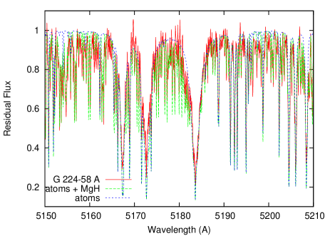
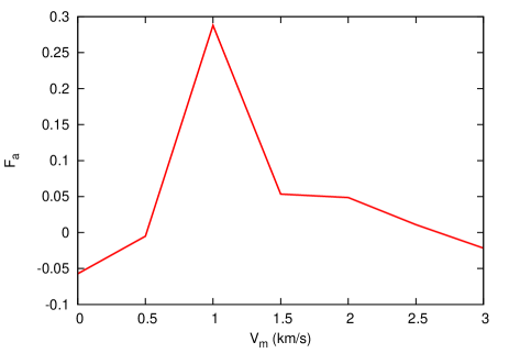
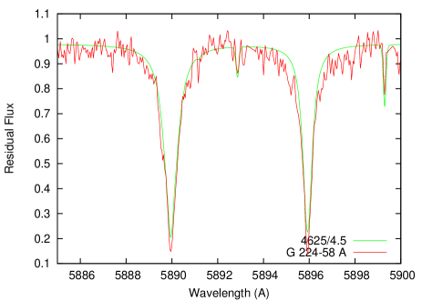
Figure 1: Top: fits of the observed in spectrum G 224-58 A Mg I line triplet and MgH lines Labels ’atoms’ and ’atoms+MgH’ mark synthetic spectra computed with account of atomic lines and atomic lines + MgH, respectively. Middle: dependence of $F_{\rm a}$ on $V_{\rm m}$ for Fe lines, model atmosphere 4625/4.5. Bottom: fits to Na I resonance doublet.

We used the Sun as a template star in this study applying our technique to determine solar abundances in order to give reliability to our abundances for G 224-58 A . We used an observed solar spectrum with resolution R $>$ 100,000 from Kurucz et al. (1984). The abundances are determined for a list of pre-selected lines which are fitted well in the solar spectrum and for the Sun we adopt T_eff/$log$ g/[Fe/H]=5777/4.44/0.00 (see Pavlenko et al. 2012)). The abundances we obtained are in good agreement with known classical results, e.g. Anders & Grevesse (1989); Gurtovenko & Kostik (1989) within $\pm$ 0.1 dex. Further details of the procedure are given in Kushniruk et al. (2014).

3.2 Modelling G 224-58 A optical spectrum

From the literature, we expect that the effective temperature of G 224-58 A is in the 4500 - 4750 K range and that the atmosphere is metal deficient. We carried out our abundance determination of the star applying the procedure described in the section 3.1 for model atmospheres of $T_{\rm eff}$ = 4500 and 4750 K, log g = 4.5 and 5.0. These computations provide rather similar results, i.e [Fe/H] $\sim$ -2.0. We probed these solutions with analysis of the spectral region where strong lines of Mg I and the $A\leavevmode\nobreak\ ^{2}\Pi\leavevmode\nobreak\ -\leavevmode\nobreak\ X\leavevmode\nobreak\ ^{2}\Sigma^{+}$ band system of MgH molecule are located, see the upper panel of Fig. 1. These features in the synthetic spectra show a notable dependence on the gravity chosen (Kushniruk et al. 2013). Additionally we determined the titanium abundance log N(Ti) using the lines of different titanium ions, i.e. Ti I and Ti II. We found formally similar results of abundance determinations for the cases of 4500/4.5 and 4750/5.0. However, MgH lines were too strong in the case of 4500/4.5 and too weak in the case of 4750/5.0, and abundances obtained from the fits to Ti I and Ti II lines disagree by more than 0.1 dex with each other, see Section 3.2.3.

We checked $T_{\rm eff}$ = 4625 K, and log g = 4.5–5.0 models. Since 4625/4.5 model matches better both the MgH lines and the minimal disagreement between Ti I and Ti II abundances (see section 3.2.3), we choose it for our further analysis.

3.2.1 Microturbulent velocity $V_{\rm m}$ 

The procedure of microturbulent velocity determination differs from that described in Pavlenko et al. (2012) as follows.

• We determine a small grid of $N_{v}$ microturbulent velocities $V_{m}=V_{0}+i*0.5$, $i$ changes from 1 to 7. We adopt $V_{0}$ = 0 km/s and so cover a grid of plausible values for $V_{\rm m}$ in the atmospheres.

• For every microturbulent velocity from our grid we obtained the iron abundances $logN_{k}(Fe),k=1,\dotsc L,$ here $L$ is the number of lines in our pre-selected list, and determined the central residual fluxes of fitted lines $r_{\lambda_{0}^{k}}$.

• Using $\chi^{2}$ fitting, we approximate the dependence of log N(Fe) vs. $r_{\lambda_{0}}$ by the linear formula $logN(Fe)=A$ + $F_{\rm a}$ * $(r_{\lambda_{0}})$, here $A$, $F_{\rm a}$ are constants which depend on $V_{\rm m}$ . We are interested in the case $F_{\rm a}$ = 0, when all lines provide the same abundances.

A similar approach for $V_{\rm m}$ determination from the equivalent width vs. abundance analysis was used by R. Kurucz in his WIDTH9 code. However, our approach is more flexible in the sense that we can use $V_{\rm m}$ determination even for blended lines.

In the middle panel of Fig. 1 we see $F_{\rm a}$ = 0 at least at $V_{\rm m}$ =0.5 and 2.5 km/s. Corresponding abundances of iron obtained from the fits to profiles of 44 lines of Fe I in the spectrum of the primary are -6.290 $\pm$ 0.021 and -6.478 $\pm$ 0.026, respectively. We choose the first value due to the lower dispersion of results. It is worth noting, that $V_{\rm m}$ = 0.5 km/s seems to be reasonable from the point of view that the lower opacity photospheres of metal poor stars allow spectra to probe deeper, i.e. into higher pressure layers where we cannot expect high velocity motions/large $V_{\rm m}$ .

3.2.2 Fit to sodium resonance doublet

Sodium lines are of special interest as they form strong features in the spectra of both G 224-58 A and G 224-58 B . In the primary spectrum we see the strong lines of the resonance doublet of Na I at 5889.95 and 5895.92 Å. Their intensities depend on $T_{\rm eff}$ , $\log\leavevmode\nobreak\ g$ , $V_{\rm m}$ and the sodium abundance. In the bottom panel of Fig 1 we show the fit of our synthetic spectra to the Na I doublet line profiles observed in G 224-58 A spectrum. Both lines are better fitted with the model atmosphere $T_{\rm eff}$ = 4625, log g =4.5 with N(Na) = -7.34, i.e, we obtain [Na/Fe] = -0.2 for the primary.

3.2.3 Fit to Ti II lines in the observed spectrum of G 224-58 A 

The abundance ratio of ionized species of the same element, usually Fe I/Fe II, is known to change with $\log\leavevmode\nobreak\ g$ for a fixed $T_{\rm eff}$ and therefore it is often used to verify the selection of $\log\leavevmode\nobreak\ g$ , serving to constrain the global solution. However, our primary G 224-58 A is metal deficient and a relatively cool star. In comparison with the Sun, it is difficult to locate appropriate lines of Fe II. We found a few features consisting of weak and blended Fe II lines, but results of their fit was not confident due to the low quality of the observed spectrum.

On the other hand, due to the lower ionization potential of the neutral titanium $(E=6.83eV)$ in comparison to Fe I $(E=7.90eV)$, the lines of Ti II should be stronger in spectra of comparatively cooler stars, i.e., more useful for abundance analysis. Therefore we used lines of Ti I and II to make the analysis instead. Indeed, we found lines of Ti II which are fit well in our synthetic spectra and list in Table 1. To be more confident, we also looked at these lines in spectrum of the Sun finding a good agreement between the lines in model atmosphere 5777/4.44/0 from Pavlenko (2003) and observations from the Kurucz et al. (1984) atlas, see Fig. 2. The good agreement between abundances found using Ti I vs Ti II gives additional independent support in our choice for the G 224-58 A model atmosphere parameters.

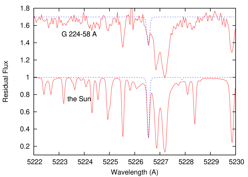
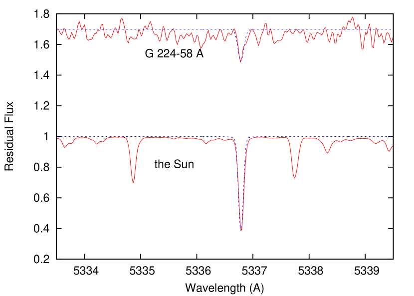
Figure 2: Fit of our theoretical Ti II lines to the observed spectra of the G 224-58 A and the Sun. In the theoretical spectra only absorption by Ti II is included. Spectra of G 224-58 A are shifted vertically to simplify the plots.

3.2.4 Other elements

Table 1: Fitted Ti II lines in spectra of G 224-58 A and the Sun, spectroscopic data were taken from VALD3.

Wavelength, Å	gf	E${}^{\prime\prime}(eV)$
5129.16	4.571E-02	1.892
5226.54	5.495E-02	1.566
5336.79	2.512E-02	1.582
5381.02	1.072E-02	1.566
5418.77	7.413E-03	1.582

Table 2: Abundances of elements determined from fits to G 224-58 A hires spectrum. $l$ and $L_{total}$ are a number of accounted lines and the total number of lines in pre-selected line list $L$, respectively. Sensitivity of abundances on the changes of parameters of model atmosphere with respect to the model 4625/4.5/-1.5^∗, $V_{\rm m}$ = 0.5 km/s model is shown in the latter columns.

Elem	$z$	log N(x)	[X/H]	$v$ sin $i$	$l/L_{total}$	$\Delta$ $V_{\rm m}$ = +0.5 km/s	$\Delta$ $\log\leavevmode\nobreak\ g$ = 0.5	$\Delta$ $T_{\rm eff}$ = -100 K
Mg	12	-5.972	-1.512	2.33 $\pm$ 0.42	6/7	0.003	-0.007	0.087
Ca	20	-7.067	-1.387	2.66 $\pm$ 0.14	16/16	0.038	0.012	0.107
Ti	22	-8.422	-1.372	2.25 $\pm$ 0.21	14/16	0.029	-0.068	0.114
Cr	24	-8.254	-1.884	2.83 $\pm$ 0.12	9/9	0.089	0.033	0.167
Mn	25	-8.609	-1.959	2.50 $\pm$ 0.32	5/5	0.040	-0.100	0.080
Fe	26	-6.290	-1.920	2.50 $\pm$ 0.10	44/44	0.051	-0.094	0.090
Ni	28	-7.598	-1.808	1.89 $\pm$ 0.32	9/9	0.089	-0.134	0.092
Ba	56	-11.780	-1.870	1.88 $\pm$ 0.38	4/4	0.125	-0.125	0.166

Abundances determined from selected line lists are shown in the Table 2. In the 6-th column of the table we show the number of preselected line lists and number of accounted lines. In particular we note that that light $\alpha-$elements Mg, Ca, Ti are overabundant in comparison with elements of iron peak Cr, Mn, Fe, Ni, Ba. For this analysis we use the weaker lines, i.e not ones that we find to be saturated in the observed spectrum. Table 2 indicates that the uncertainties of the abundances do not exceed 0.17 dex for the adopted range of parameter variation.

The found overabundance of Mg, Ca, Ti with respect to the Fe shows rather weak dependence on the choice of $T_{\rm eff}$ , $\log\leavevmode\nobreak\ g$ or $V_{\rm m}$ , see Table 2. In general, the overabundance of alpha-elements is a well known phenomenon for metal-deficient stars, e.g., Magain (1987); McWilliam (1997); Sneden (2004), or more recently Hansen et al. (2015).

To carry out the process of abundance analysis we fitted the observed profiles of the spectral lines. This procedure allows us to determine the rotational velocity $v$ sin $i$ . It is worth noting that the values of $v$ sin $i$ in Table 2 should be considered rather as upper limits due to the natural restrictions provided by the limited quality of our observed spectrum. In some sense $v$ sin $i$ is used here as the adjusting parameter of our fitting procedure. For more a accurate determination of $v$ sin $i$ we should adopt/develop more sophisticated models of instrumental broadening and macroturbulence and use them for fits to the observed spectra of better quality. For now we can claim that G 224-58 A is a slowly rotating ($v$ sin $i$ $<$ 3 km/s) star, this agrees well with its status of old halo star.

3.3 LIRIS infrared spectrum of G 224-58 A 

Fits to LIRIS low resolution (R=2500) spectra observed in $H,J,K$ spectral ranges are shown in Fig. 3. The Figure shows the observed spectra, where we overplotted the theoretical spectra (blue and green lines), for two different Silicon abundances. The theoretical spectra were computed by using the optical G 224-58 A spectrum (see section 3.2).

Despite the comparatively low resolution, we are able to identify a few Si I lines in the observed spectra. In the Fig. 3 we show two cases, with [Si] =–1.0 and –2.0. It is apparent that Si=–1.0 is a better fit and thus Si I is overabundant. Si (Z=14) belongs to the alpha-element group and as discussed earlier its overabundance is expected. Here we can claim only an estimation of Si overabundance, i.e. [Si/H] $\sim$ –1.1 $\pm$ 0.3 dex based on an average of the line fits. Here we note that changes of Si abundance by factor 10 affects the general shape of the observed SEDs (Fig 3). Si I is an important donor of free electrons in cool atmospheres, therefore both model atmospheres and computed spectra show dependence on its abundance. Unfortunately, the absorption lines of Si I are too weak to discern in our optical spectrum of G 224-58 A lower limit.

In the $H$ spectral region we see a strong Mg I line at 15754 Å. We obtained a fit to this line with the Mg abundance obtained from the analysis of optical spectrum. In fact, this provides independent confirmation of our results in Table 2.

In the $K$ spectral region we can discern the presence of the CO overtone bands at the expected level but not sufficiently well to determine the carbon abundance.

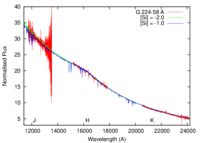
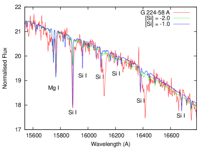
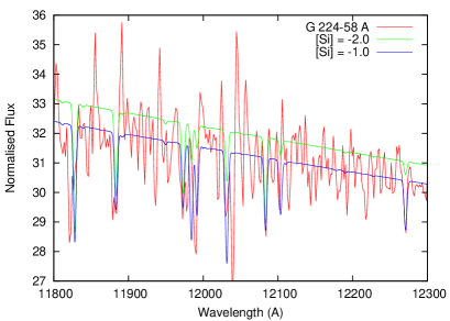
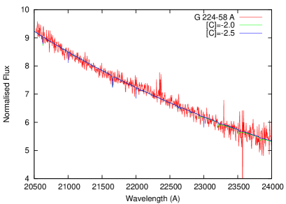
Figure 3: Fit to G 224-58 A LIRIS infrared spectrum (top left). Three others plots show fits to the observed $H$ (top right), $J$ (bottom left), $K$ (bottom right) spectral regions in larger scale

4 G 224-58 B spectrum analysis

4.1 Procedure

G 224-58 B is a late spectral type dwarf. In general we will assume that, as a binary the B component has the same properties of age and composition that we have found for A component. However, we perform a different approach to metallicity determination.

First, we generated a grid of the LTE synthetic spectra following the procedure outlined in Pavlenko (1997). We started with the NextGen model atmospheres of effective temperatures 2800, 2900, 3000, 3100, 3200, 3300, 3400 K, gravities of log g = 4.0, 4.5, 5.0, 5.5 and metallicities [Fe/H] = –1.5 and 2.0. We replaced some abundances by the values obtained for the G 224-58 A with parameters $T_{\rm eff}$ =4625 K, $\log\leavevmode\nobreak\ g$ =4.5. In our computations the line lists of VO and CaH were taken from Kurucz’s website, for more details see Pavlenko (2014). The CrH and FeH line lists were computed by Burrows et al. (2002) and Dulick et al. (2003), respectively. We upgraded the TiO line lists of Plez (1998) with the new version available on his website. Infrared spectra were computed with account of water vapour absorption lines provided by the EXOMOL group Barber et al. (2006). The spectroscopic data for atomic absorption VALD3 come from the Vienna Atomic Line Database Kupka et al. (1999). The profiles of the NaI and KI resonance doublets were computed here in the framework of a quasi-static approach described in Pavlenko et al. (2007) with an upgraded approach from Burrows & Volobuyev (2003). More details on the technique and procedure are presented in Pavlenko et al. (2006).

4.2 Results of the G 224-58 B optical spectrum analysis

In Fig. 4 we show a compilation of the main absorption features that can be observed in the spectrum of G 224-58 B . The main feature is formed by CaH $A^{2}\Pi_{r}-X^{2}\Sigma^{+}$band system. Strong MgH, TiO band systems and K I and Na I resonance lines also form noticeable features in the secondary spectrum.

The choice of best fit between the observed and computed spectra was achieved by minimizing the parameter

$$S(f_{\rm h})=\sum_{\nu}\left(F_{\nu}-F_{\nu}^{x}\right)^{2},$$

where $F_{\nu}$ and $F_{\nu}^{x}$ are the fluxes in the observed and computed spectra, respectively, and $f_{\rm h}$ is the normalization factor. A similar procedure was used by Pavlenko et al. (2006). Fits were made for all synthetic spectra in our grid. We use the instrumental resolution $R=1500$ for our calculations.

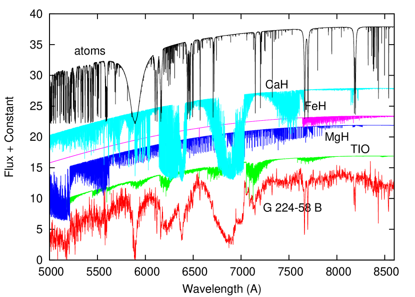
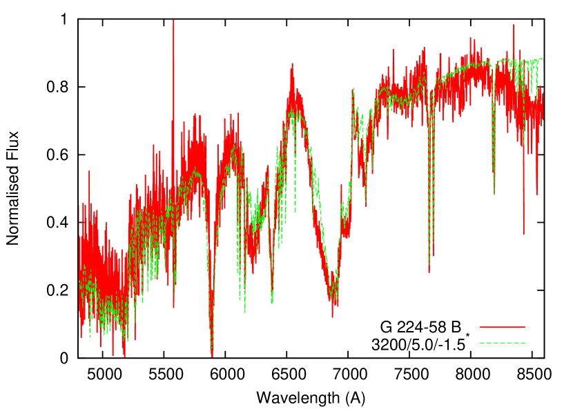
Figure 4: Left: identification of the main molecular features formed the observed optical spectrum of the B component, model atmosphere 3200/5.0/-1.5^∗ from NextGen grid (Hauschildt et al. (1999)). Right: fit of our synthetic spectrum computed with the same model atmosphere to the observed SED of G 224-58 B .

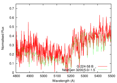
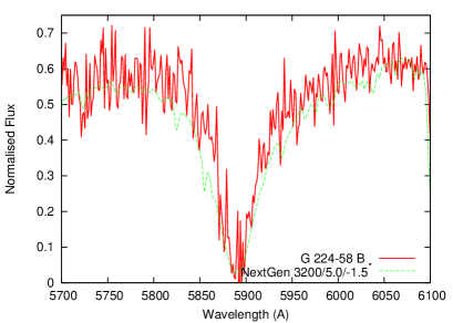
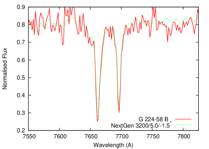
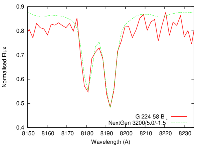
Figure 5: Fits of some spectral details in our theoretical spectra shown in the right panel of the Fig 4 to the observed features in G 224-58 B spectrum: MgH $A\leavevmode\nobreak\ ^{2}\Pi\leavevmode\nobreak\ -\leavevmode\nobreak\ X\leavevmode\nobreak\ ^{2}\Sigma^{+}$ band system at 5200 Å(top left), lines of Na I resonance doublet (top right), lines of resonance doublet of K I (bottom left), subordinate lines of Na I (bottom right). Model atmosphere and normalization point are the same as for Fig 4.

The best fit of our synthetic spectrum to the G 224-58 B observed SED is obtained for the 3200/5.0/-1.5^∗ model atmosphere (see Fig. 5). Abundance scaling parameter -1.5^∗ means here that a reducing factor -1.5 was used for all abundances in the NextGen model atmosphere except for those obtained from the analysis of the primary spectrum. Then, we used ”the best fit” (as defined previously) to describe the best agreement between the computed and observed SED and the profiles of strong lines. Fig. 5 shows the fit to the observed SEDs and intensities of the strong sodium and potassium lines, with abundances obtained from analysis of G 224-58 A spectrum.

4.2.1 Strong features in the G 224-58 B spectrum

The notable features in the observed spectrum are formed by MgH $A\leavevmode\nobreak\ ^{2}\Pi\leavevmode\nobreak\ -\leavevmode\nobreak\ X\leavevmode\nobreak\ ^{2}\Sigma^{+}$ band system at 5200 Å, CaH $A^{2}\Pi_{r}-X^{2}\Sigma^{+}$and $B/B^{\prime}2\Sigma^{+}-X^{2}\Sigma^{+}$band systems in the wide spectral range, as well as TiO $\gamma$ band system at 7200 Å. We see that these features in the observed spectrum are well reproduced by our theoretical computations with the abundance obtained from G 224-58 A analysis.

Furthermore, in the observed G 224-58 B spectrum we see sodium and potassium resonance doublet lines at 5890 and 7680 Å, as well as sodium triplet lines at 8190 Å known as a good gravity discriminator. In Fig.5 we show our fits to these observed K I and Na I lines. To reproduce Na I lines in G 224-58 B spectrum we used the sodium abundances determined from analysis of G 224-58 A spectrum.

The potassium resonance lines are beyond the spectral range observed for the G 224-58 A , and other potassium lines are very weak. Still we see strong lines of potassium doublet in G 224-58 B observed spectrum. To fit these lines we used the same abundance scaling factor, as was found for sodium, i.e. [K/Fe] = –0.2 and obtained good agreement between observed and computed profiles. It would be interesting to verify this result by the comparison of computed and observed profiles of potassium resonance doublet in the G 224-58 A spectrum.

4.2.2 Fe lines

Since iron lines in G 224-58 A spectrum are numerous, the determination of Fe abundance was done with high accuracy. Ideally a similar analysis would be performed for the G 224-58 B , using the same FeI line list. However, practically its lower effective temperature, where molecular bands dominate the spectrum combined with the lower resolution and signal-to-noise make this difficult. The lines are at the level of the noise. We could use only the Fe I line at 5325.19 Å. We only can claim that weak Fe I lines are present in the observed spectrum and based on Fig 7 find [Fe/H] = –1.7.

4.3 Fit to LIRIS spectra of G 224-58 B 

The LIRIS infrared spectrum of G 224-58 B has comparatively low signal-to-noise. Therefore, to reduce the level of noise we binned the observed spectrum by a factor of 7. In the following we show the binned spectra to simplify.

Synthetic spectra were computed for the model atmosphere 3200/5.0/-1.5^∗ with a 0.05 Å step taking into account all known molecular opacity sources. First of all we computed the contribution of the molecular bands to the opacity in our spectral ranges. Results are shown in the left panel of Fig 6. Water vapour absorption dominates across all modelled spectral ranges. In the most general case absorption by H₂O depends on effective temperature, oxygen abundance and other input parameters. In our work we fixed almost all of these parameters, so we have a chance to estimate the oxygen abundance. Indeed, the shape of the computed SEDs across the H band depends on the water absorption, with better agreement when we adopt some underabundance in the atmosphere of the B component, see the right panel of Fig. 6.

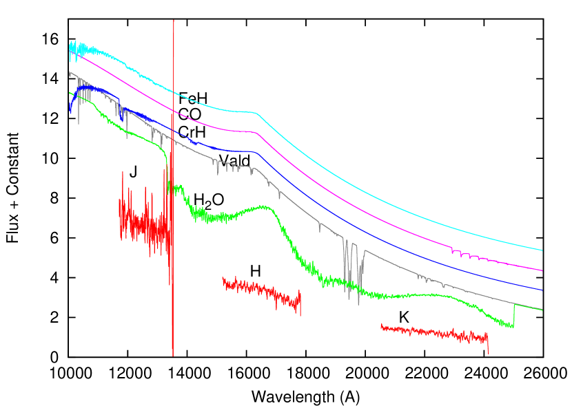
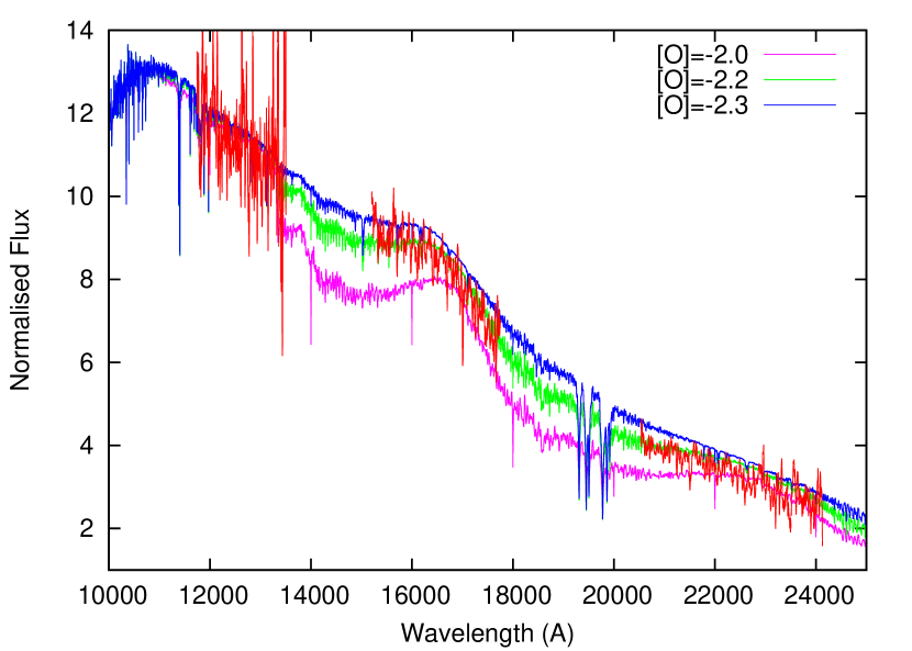
Figure 6: Left: identification of the main molecular features formed the observed by LIRIS infrared spectrum of the B component, model atmosphere 3200/5.0/-1.5^∗. ”Vald” marks the synthetic spectrum computed for atomic line list. ”H”, ”J”, ”K” mark three spectral ranges observed by LIRIS. Right: fit of our synthetic spectra computed with the same model atmosphere, but different oxygen abundances, to the observed SED of G 224-58 B .

4.4 Fit of BT-Settl spectra to the optical and infrared SEDs of G 224-58 B 

Here we computed synthetic spectra for model atmospheres from the NextGen grid (Hauschildt et al. 1999) as newer BT-Settl model atmosphere are not in the public access. Nonetheless, fluxes for a fixed grid of abundances are available and we used them for the comparison with our observed spectra.

In Fig. 8 we provide fits of the BT-Settl spectra computed with 3150/5.0/-1.5 model atmosphere to the observed fluxes of G 224-58 B . Here the metallicity parameter [Fe/H] = -1.5 was used to adjust all abundances. As can be seen, BT-Settl fluxes reproduced well the observed SEDs. Also the Ca, Mg and Ti abundances adopted in BT-Settl model agree well with our values, obtained from the fits to the A component. Therefore CaH, MgH and TiO bands are fitted well enough with both our model with modified abundances and an original BT-Settl model. We should remark that the NextGen and BT-Settl model atmospheres should be similar. Indeed, dusty effects at these relatively warm temperatures from the BT-Settl model atmosphere will be very minor, given the case of similarity of the main opacity sources we should get similar results.

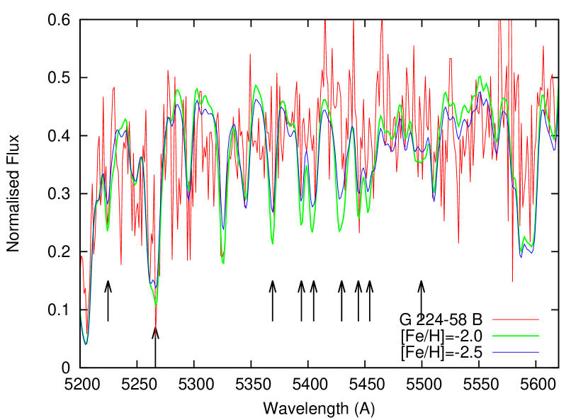
Figure 7: Fit of our computed 3200/5.0/-1.5^∗ model atmosphere theoretical spectrum to the observed G 224-58 B spectrum. NIR spectra were smoothed here by 3 pixels for clarify. Vertical arrows mark positions of Fe I lines in the computed spectrum.

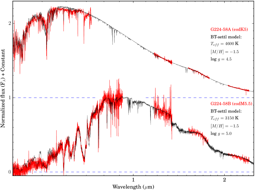
Figure 8: Spectra of G 224-58 AB compared to BT-Settl model spectra. Spectra are normalised at 0.82 $\mu$m.

5 Discussions and conclusions

Our final results of abundance determination in atmospheres of G 224-58 A and G 224-58 B are shown in Table 3. Here we compiled abundances obtained by fits to our spectra across optical and infrared spectral ranges, using different approaches to get the best fits to observed absorption profiles and spectral features. In that way we obtained the fits to G 224-58 A and G 224-58 B spectra using the same abundances.

Table 3: Abundances determined for the atmospheres of G 224-58 A and G 224-58 B . The errors given for G 224-58 A are determined by our minimisation procedure and for G 224-58 B are made “by-eye”.

Element	$Z$	log N	$[X/H]_{A}$	$[X/H]_{B}$
O	8	-5.3		-2.1 $\pm$ 0.2
Na	11	-7.87	-2.1 $\pm$ 0.2	-2.1 $\pm$ 0.2
Mg	12	-5.975	-1.512 $\pm$ 0.079	-1.5 $\pm$ 0.1
Si	14	-5.59		-1.1 $\pm$ 0.3
K	19	-9.0		-2.1$\pm$ 0.2
Ca	20	-7.105	-1.387 $\pm$0.025	-1.4 $\pm$ 0.2
Ti	22	-8.451	-1.372 $\pm$ 0.028
Cr	24	-8.343	-1.884 $\pm$ 0.065
Mn	25	-8.649	-1.959 $\pm$ 0.055
Fe	26	-6.341	-1.920 $\pm$ 0.020	-1.9 $\pm$ 0.5
Ni	28	-7.687	-1.808 $\pm$ 0.050
Ba	56	-11.905	-1.870 $\pm$ 0.111

Zhang et al. (2013) provided very strong arguments about the binarity of G 224-58 AB, based on the common high proper motion (PM) and radial velocity (RV). We used their results as a starting point for our investigation. Our study provides confirmation about the binary nature of the objects through the consistency of the abundance measurements of the A and B components.

From our analysis of the primary spectrum (see Table 2) we determined [Mg/Fe] = +0.41$\pm$0.05, [Ca/Fe] = +0.53$\pm$0.05, [Ti/Fe] = +0.55$\pm$0.05, i.e. these elements are overabundant relative to iron. Our finding is confirmed by direct modeling of the cool secondary dwarf spectra. Generally speaking, the overabundance of Ca in atmospheres of metal poor stars is well known (see Magain 1987; McWilliam 1997; Sneden 2004, and references therein). In the case of binary systems, or exoplanetary systems the situation looks even more intriguing, because here we have the impact of a few very different processes: early epoch nucleosynthesis, separation of heavy elements in the binary system process formation, etc. An interesting aspect of studying halo systems including a cool component like G 224-58 AB is that it provides an opportunity for the abundance determination of some elements, e.g. K and Na.

Generally speaking, for [Fe/H] $>$ -1.0 there is not much variation in abundance ratios for different elements at any given [Fe/H] for single (non-binary) main sequence stars, so that knowing [Fe/H] does give us a good idea what its abundances are for other elements, e.g., figures 9, 10, and 11 in Reddy et al. (2003). Besides, for lower metallicity stars there is more scatter in the [X/Fe] ratio for some elements for a given [Fe/H], which may affect the stellar atmosphere, e.g. two stars with [Fe/H] = -1.5 but with very different alpha element abundances will have different line opacity.

The essential result of our G 224-58 A spectrum analysis is the conclusion that at least for the case of metal deficient stars with [Fe/H] $<$ -1.0 we cannot use one parameter, the metallicity, to describe the behaviour of individual abundances. This conclusion agrees well with Woolf et al. (2009) results and demonstrates the importance and necessity of abundance analysis of binaries like G 224-58 AB. Comparison of our results for Ti with Woolf et al. (2009) abundances for esdM shows at least a good qualitative agreement. For the most metal poor esdM LP 251-35 (3580/5.0/-1.96) they obtained [Ti/Fe] = 0.45. Interestingly, these authors used K I and Ca II lines to determine the parameters of the atmosphere of the stars. Here we have obtained an overabundance in calcium and under abundance of potassium (and sodium) in the atmosphere of G 224-58. If the overall abundances of the extremely metal-poor M-dwarfs are similar, their results may be affected by abundance uncertainties.

Lépine et al. (2007) defined a metallicity index, $\zeta_{\rm TiO/CaH}$, which is formed by a combination of the spectral indices of TiO5, CaH2, and CaH3. They classified M subdwarfs into three metal classes: subdwarf (sdM; $0.5<\zeta_{\rm TiO/CaH}<0.825$), extreme subdwarf (esdM; $0.2<\zeta_{\rm TiO/CaH}<0.5$ ) and ultra subdwarf (usdM; $\zeta_{\rm TiO/CaH}<0.2$). Metallicity measurements of M subdwarfs have been conducted with high resolution spectra (Woolf & Wallerstein 2006; Woolf et al. 2009; Rajpurohit et al. 2014). The relationship between the $\zeta_{\rm TiO/CaH}$ and [Fe/H] has been studied (Woolf et al. 2009; Mann et al. 2013; Rajpurohit et al. 2014). We calculated the metallicity index $\zeta_{\rm TiO/CaH}$ = 0.22 for G 224-58 B to compare to previous works.

Figure 9 shows the $\zeta_{\rm TiO/CaH}$ and [Fe/H] of G 224-58 B and M subdwarfs from Woolf et al. (2009). A blue dashed line in Figure 9 represents the correlation of $\zeta_{\rm TiO/CaH}$ and [Fe/H] for late-type K and early-type M subdwarfs (3500-4000 K) (Woolf et al. 2009). A black solid line represents our fitting of G 224-58 B and M subdwarfs from Woolf et al. (2009), which can be described with [Fe/H] = 2.004 $\times\zeta_{\rm TiO/CaH}-1.894$. We excluded objects from Rajpurohit et al. (2014) in our fitting because to reduce the dispersion of results in Fig. 9 would require a shift of [Fe/H] values from Rajpurohit et al. (2014) by a factor of –0.3 to –0.5 downward. This could arise from the overabundance of Ti and Ca and their inclusion in the [Fe/H] values they compute.

It is worth noting that:

• Rajpurohit et al. (2014) measure [Fe/H] with only iron lines, however, for three M dwarfs shown in fig. 11 of Rajpurohit et al. (2014) they find $\zeta_{\rm TiO/CaH}>$ 0.825 for metallicities from $-$0.5 to $-$1.0 and so these values are significantly discrepant for the $\zeta_{\rm TiO/CaH}$ parameter. We note their fit to the sdM9.5 object in a small region of optical spectrum gave [Fe/H] = -1.1 and $T_{\rm eff}$ = 3000K. From the fit to the 0.7-2.5 $\mu$m NIR spectrum of the same object with same model, we got [Fe/H] = -1.6 and $T_{\rm eff}$ = 2700K. We note that an analysis of a narrow spectral region can be significantly impacted by relatively different pseudocontinuums formed by molecular bands in the optical and the infrared. The measurement of abundance and temperature from atomic line strength can be significantly impacted by such differences, e.g., (see Pavlenko et al. 1995).

• Woolf’s results of $\zeta_{\rm TiO/CaH}$ determination are affected by uncertainties in the adopted K, Na, Ca and Mg abundances.

• Our value of iron abundance obtained for the G 224-58 A in the analysis explained in previous sections is [Fe/H] = -1.920; only one M subdwarf from Woolf et al. (2009) has lower [Fe/H] than G 224-58 B but was excluded in their fitting.

For the case of halo dwarfs of later spectral classes, i.e. esdM dwarfs, the use of one parameter of metallicity may seriously impact results. And, this is why we need binaries to calibrate spectral indices vs. abundance dependence for M subdwarfs of different populations.

In general, our fits to the infrared spectra of the G 224-58 A and G 224-58 B observed with LIRIS provide the independent confirmation of the correctness of our choice of parameters of atmospheres of both components. With the spectrum of G 224-58 B , we find evidence of overabundance of Si I and underabundance of oxygen. It is worth nothing these results were obtained by fitting to low resolution infrared spectra. In spectra of stars of normal metallicity the results are affected by the presence in the spectral analysis of complex blending. However, in the case of metal deficient stars these effects are less pronounced. Moreover, in our case we have not any other chance to estimate oxygen and silicon abundances, except through the modelling of infrared spectra. To analyse weak oxygen and silicon lines in the optical spectrum of A component we require the spectral data of a quality comparable with solar atlas. The underabundance found in oxygen may be explained as a real small number of atoms in the primary atmosphere due to its association in CO when the carbon abundance/presence is comparatively high in the atmosphere. Our picture could be better tested if were able to do more precise analysis of the CO bands at 2.3 micron.

The abundance inhomogeneities found can be most easily explained in terms of the nucleosynthesis of halo stars at their formation epoch. The low iron abundance, i.e [Fe/H] = -1.92, together with large PM determined by Zhang et al. (2013) allows assignment of G 224-58 AB to the halo population. We detect in the atmospheres of G 224-58 AB, overabundances with respect to the iron, not only of Ti, but also of other alpha-element elements. The study of similar systems, their physical characteristics as well as their multiplicity, is of crucial importance for the investigation of binary and multiple system formation processes and their evolution through composition and time, including the formation of still hypothetical exoplanetary systems in the early epochs of Galaxy evolution.

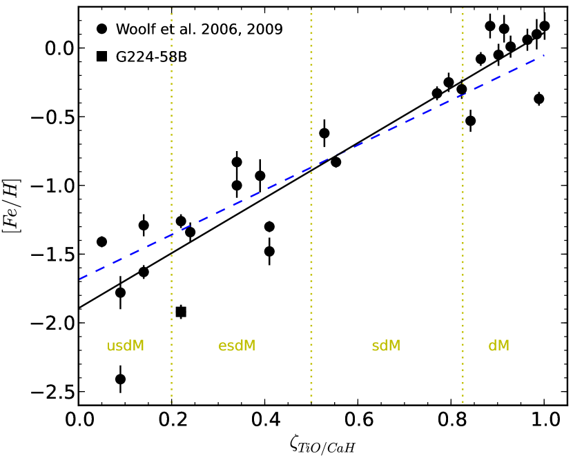
Figure 9: Metallicity parameter $\zeta_{\rm TiO/CaH}$ vs. [Fe/H] for G 224-58 B and M subdwarfs from Woolf & Wallerstein (2006), Woolf et al. (2009). The blue dashed line represents the fitting from Woolf et al. (2009). The black solid line represents our fitting of G 224-58 B and data from Woolf & Wallerstein (2006); Woolf et al. (2009). The fit can be described with $[Fe/H]=2.004\times\zeta_{\rm TiO/CaH}-1.894$. Red dotted lines shows the boundaries of metallicity classes of M dwarfs from Lépine et al. (2007).

6 Acknowledgments

Based on observations made with the Nordic Optical Telescope, operated by the Nordic Optical Telescope Scientific Association at the Observatorio del Roque de los Muchachos, La Palma, Spain, of the Instituto de Astrofísica de Canarias. The WHT and its service programme are operated on the island of La Palma by the Isaac Newton Group in the Spanish Observatorio del Roque de los Muchachos of the Instituto de Astrofísica de Canarias. M.C. Gálvez-Ortiz acknowledges the financial support of a JAE-Doc CSIC fellowship co-funded with the European Social Fund under the programme ”Junta para la Ampliación de Estudios” and the support of the Spanish Ministry of Economy and Competitiveness through the project AYA2011-30147-C03-03. The authors thank the compilers of the international databases used in our study: SIMBAD (France, Strasbourg), and VALD (Austria, Vienna) and R. Kurucz and Phoenix group for model atmospheres, synthetic spectra. We thank Jose Antonio Acosta Pulido for his helps with the LIRIS data reduction. We thank the anonymous Referee for his/her thorough review and highly appreciate the comments and suggestions, which significantly contributed to improving the quality of the publication.

References

- Anders & Grevesse (1989) Anders, E. & Grevesse, N. 1989, Geochim. Cosmochim., Acta 53, 197
- Bean et al. (2006) Bean, J. L., Benedict, G. F., Endl, M. 2006, ApJ, 652, 1604.
- Barber et al. (2006) Barber, R. J., Tennyson, J., Harris, G. J., Tolchenov, R. N. 2006, MNRAS, 368, 1087
- Bowler et al. (2009) Bowler, B. P., Liu, M. C. & Cushing, M. C. 2009, ApJ, 706, 1114
- Burningham et al. (2009) Burningham, B., Pinfield, D. J., Leggett, S. K. et al. 2009, MNRAS, 395, 1237
- Burningham et al. (2010) Burningham, B., Leggett, S. K., Lucas, P. W. et al. 2010, MNRAS, 404, 1952
- Burrows & Volobuyev (2003) Burrows, A. & Volobuyev, M. 2003, ApJ, 583, 985
- Burrows et al. (2002) Burrows, A., Ram, R. S., Bernath, P., Sharp, C. M. & Milsom, J. A. 2002, ApJ, 577, 986
- Dulick et al. (2003) Dulick, M., Bauschlicher, C. W., Jr., Burrows, A. et al. 2003, ApJ, 594, 651
- Faherty et al. (2010) Faherty, J. K., Burgasser, A. J., West, A. A. et al. 2010, AJ, 139, 176
- Gizis (1997) Gizis, J. E. 1997, AJ, 113, 806
- Gray (1976) Gray, D.F. 1976, The observation and analysis of stellar photospheres. New York, Wiley-Interscience, 484 p.
- Gurtovenko & Kostik (1989) Gurtovenko, E. A., Kostik, R. I. 1989, Naukova Dumka, 1.
- Hansen et al. (2015) Hansen, T., Hansen, C.J., Christlieb N. 2015, astro-ph:1506.00579v1.
- Hauschildt et al. (1999) Hauschildt, P. H., Allard, F. & Baron, E. 1999, ApJ, 512, 377
- Jao et al. (2008) Jao, W.-C., Henry, T. J., Beaulieu, T. D. & Subasavage, J. P. 2008, AJ, 136, 840
- Kupka et al. (1999) Kupka, F., Piskunov, N., Ryabchikova, T. A., Stempels, H. C., & Weiss, W. W. 1999, A&AS, 138, 119
- Kurucz et al. (1984) Kurucz, R. L., Furenlid, I., Brault, J., & Testerman, L. 1984, National Solar Observatory Atlas, Sunspot, New Mexico: National Solar Observatory
- Kurucz (1993) Kurucz, R. 1993, ATLAS9 Stellar Atmosphere Programs and 2 km/s grid. Kurucz CD-ROM No. 13. Cambridge, Mass.: Smithsonian Astrophysical Observatory, 1993., 13
- Kushniruk et al. (2013) Kushniruk, I. O., Pavlenko, Y. V., & Kaminskiy, B. M. 2013, Advances in Astronomy and Space Physics, 3, 29
- Kushniruk et al. (2014) Kushniruk, I. O., Pavlenko, Y. V., Jenkins, J. S. & Jones, H. R. A. 2014, Advances in Astronomy and Space Physics, 4, 20
- Lépine et al. (2007) Lépine, S., Rich, R. M. & Shara, M. M. 2007, ApJ, 669, 1235
- López-Morales (2007) López-Morales, M. 2007, ApJ, 660, 732
- Luhman et al. (2007) Luhman, K. L., Patten, B. M., Marengo, M. et al. 2007, ApJ, 654, 570
- Magain (1987) Magain, P. 1987, A&A, 179, 176
- Manchado et al. (1998) Manchado, A., Fuentes, F. J., Prada, F., et al. 1998, SPIE, 3354, 448.
- Mann et al. (2013) Mann, A. W., Brewer, J. M., Gaidos, E., Lépine, S., & Hilton, E. J. 2013, AJ, 145, 52
- Mann et al. (2014) Mann, A. W., Deacon, N. R., Gaidos, E. et al. 2014, AJ, 147, 160
- McWilliam (1997) McWilliam, A. 1997, ARA&A, 35, 503
- Murray et al. (2011) Murray, D. N., Burningham, B., Jones, H. R. A. et al. 2011, MNRAS, 414, 575
- Neves et al. (2013) Neves, V., Bonfils, X., Santos, N. C. et al. 2013, A&A, 551, A36
- Neves et al. (2014) Neves, V., Bonfils, X., Santos, N. C. et al. 2014, A&A, 568, A121
- Newton et al. (2014) Newton, E. R., Charbonneau, D., Irwin, J. et al. 2014, AJ, 147, 20
- Önehag et al. (2012) Önehag, A., Heiter, U., Gustafsson, B., et al. 2012, A&A, 542, A33
- Pavlenko et al. (1995) Pavlenko, Y. V., Rebolo, R., Martin, E. L. & Garcia Lopez, R. J. 1995, A&A, 303, 807
- Pavlenko (1997) Pavlenko, Y. V. 1997, Ap&SS, 253, 43
- Pavlenko (2002) Pavlenko, Y. V. 2002, Kinem. and Physics of Celest. Bodies, 18, 48
- Pavlenko (2003) Pavlenko, Y. V. 2003, Astronomy Reports, 47, 59
- Pavlenko et al. (2006) Pavlenko, Y. V., Jones, H. R. A., Lyubchik, Y., Tennyson, J. & Pinfield, D. J. 2006, A&A, 447, 709
- Pavlenko et al. (2007) Pavlenko, Y. V., Zhukovska, S. V. & Volobuev, M. 2007, Astronomy Reports, 51, 282
- Pavlenko et al. (2012) Pavlenko, Y. V., Jenkins, J. S., Jones, H. R. A., Ivanyuk, O., & Pinfield, D. J. 2012, MNRAS, 422, 542
- Pavlenko (2014) Pavlenko, Y. V. 2014, Astronomy Reports, 58, 825
- Pinfield et al. (2012) Pinfield, D. J., Burningham, B., Lodieu, N. et al. 2012, MNRAS, 422, 1922
- Plez (1998) Plez, B. 1998, A&A, 337, 495
- Rajpurohit et al. (2014) Rajpurohit, A. S., Reylé, C., Allard, F. et al. 2014, A&A, 564, A90
- Reid et al. (1995) Reid, I. N., Hawley, S. L. & Gizis, J. E. 1995, AJ, 110, 1838
- Reddy et al. (2003) Reddy, B.E., Tomkin, J., Lambert, D.L., Allende Prieto, C. 2003, MNRAS, 340, 304
- Rojas-Ayala et al. (2010) Rojas-Ayala, B., Covey, K. R., Muirhead, P. S. & Lloyd, J. P. 2010, ApJ, 720, L113
- Rojas-Ayala et al. (2012) Rojas-Ayala, B., Covey, K. R., Muirhead, P. S. & Lloyd, J. P. 2012, ApJ, 748, 93
- Sneden (2004) Sneden, C. 2004, Mem. SAI, 45, 267.
- Telting et al. (2014) Telting, J. H., Avila, G., Buchhave, L., Frandsen, S., Gandolfi, D., Lindberg, B., Stempels, H. C., Prins, S., NOT staff 2014, Astronomische Nachrichten, 335, 1, p.41
- Terrien et al. (2012) Terrien, R. C., Mahadevan, S., Bender, C. F. et al. 2012, ApJ, 747, L38
- Udry et al. (1999) Udry, S., Mayor, M., & Queloz, D. 1999, IAU Colloq. 170: Precise Stellar Radial Velocities, 185, 367
- Woolf & Wallerstein (2005) Woolf, V. M., Wallerstein, G. 2005, MNRAS, 356, 96
- Woolf & Wallerstein (2006) Woolf, V. M., & Wallerstein, G. 2006, PASP, 118, 218
- Woolf et al. (2009) Woolf, V. M., Lépine, S. & Wallerstein, G. 2009, PASP, 121, 117
- York et al. (2000) York, D. G., Adelman, J., Anderson, J. E., Jr., et al. 2000, AJ, 120, 1579.
- Zhang et al. (2010) Zhang, Z. H., Pinfield, D. J., Day-Jones, A. C. et al. 2010, MNRAS, 404, 1817
- Zhang et al. (2013) Zhang, Z. H., Pinfield, D. J., Burningham, B. et al. 2013, MNRAS, 434, 1005