Gluon saturation and Feynman scaling in leading neutron production

Abstract

In this paper we extend the color dipole formalism for the study of leading neutron production in $e+p\rightarrow e+n+X$ collisions at high energies and estimate the related observables which were measured at HERA and could be analysed in future electron-proton ($ep$) colliders. In particular, we calculate the Feynman $x_{F}$ distribution of leading neutrons, which is expressed in terms of the pion flux and the photon-pion total cross section. In the color dipole formalism, the photon-pion cross section is described in terms of the dipole-pion scattering amplitude, which contains information about the QCD dynamics at high energies and gluon saturation effects. We consider different models for the scattering amplitude, which have been used to describe the inclusive and diffractive $ep$ HERA data. Moreover, the model dependence of our predictions with the description of the pion flux is analysed in detail. We demonstrate the recently released H1 leading neutron spectra can be described using the color dipole formalism and that these spectra could help us to observe more clearly gluon saturation effects in future $ep$ colliders.

I Introduction

In high energy collisions the outgoing baryons which have large fractional longitudinal momentum ($x_{L}\geq 0.3$) and the same valence quarks (or at least one of them) as the incoming particles are called leading particles (LP). The momentum spectra of leading particles have been measured already some time ago lpdata . Very recently, high precision data on leading neutrons produced in electron-proton reactions at HERA at high energies became available lpdata2 .

Leading neutron production is a very interesting process. In spite of more than ten years of intense experimental and theoretical efforts, the $x_{L}$ (Feynman momentum) distribution of leading neutrons remains without a satisfactory theoretical description holt ; bisha ; kope ; kuma ; niko99 ; models ; kkmr ; khoze ; speth ; pirner . Monte Carlo studies, using standard deep inelastic scattering (DIS) generators show lpdata2 ; monte that these processes have a rate of neutron production a factor of three lower than the data and produce a neutron energy spectrum with the wrong shape, peaking at values of $x_{L}$ below $0.3$. In order to fit the data the existing models need to combine different ingredients including pion exchange, reggeon exchange, baryon resonance excitation and decay and independent fragmentation models ; kkmr ; khoze ; speth ; pirner . Moreover, the incoming photon interacts with the pion emitted by proton and then rescatters, interacting also with the emerging neutron and giving origin to significant absorptive corrections, which are difficult to calculate speth ; pirner . As it can be seen in Fig. 1, this process is essentially composed by a soft pion (or reggeon) emission and by the subsequent photon-pion interaction at high energies. Pion emission has been studied for a long time and according to the traditional wisdom it can be described by a simple interaction Lagrangian of the form $g\bar{\psi}\gamma_{5}\pi\psi$, where $\psi$ and $\pi$ are the nucleon and pion field respectively. The corresponding pion-nucleon amplitude must be supplemented with a form factor, which represents the extended nature of hadrons and at the same time regularizes divergent integrals. The precise functional form of the form factor is very hard (if not impossible) to extract from first principle calculations. We must then resort to models. Very recently wally ; wally2 it has been argued that the Lagrangian which is more consistent with the chiral symmetry requirements is the one with a pseudovector couplings. One of the goals of the present study is to test in a new context the better founded splitting function, $f(y)$, derived in wally . Additionally, forward hadron production is very important also for cosmic ray physics, where highly energetic protons reach the top of the atmosphere and undergo successive high energy scatterings off light nuclei in the air. In each of these collisions, a projectile proton (the leading baryon) looses energy, creating showers of particles, and goes to the next scattering. The interpretation of cosmic data depends on the accurate knowledge of the leading baryon momentum spectrum and its energy dependence. A crucial question of practical importance is the existence or non-existence of the Feynman scaling, which says that the $x_{L}$ spectra of secondaries are energy independent. In cosmic ray applications we are sensitive essentially to the large $x_{L}$ region (the fragmentation region), which probes the low Bjorken-$x$ component of the target wave function. In this kinematical range nonlinear effects are expected to be present in the description of the QCD dynamics (for recent reviews see cgc ), associated to the high parton density. The state-of-art framework to treat QCD at high energies is the Color Glass Condensate (CGC) formalism CGC2 , which predicts gluon saturation at small-$x$, with the evolution with the energy being described by an infinite hierarchy of coupled equations for the correlators of Wilson lines – the Balitsky-JIMWLK hierarchy cgc . In the mean field approximation, this set of equations can be approximated by the Balitsky-Kovchegov (BK) equation BAL ; kov , which describes the evolution of the dipole-target scattering amplitude with the rapidity $Y=\ln(1/x)$.

In this paper we propose to treat the leading neutron production at HERA using the color dipole formalism, which is able to describe the inclusive and diffractive HERA $ep$ data. Our goal is to extend this successful formalism, which have its main parameters well determined, for leading neutron production. As a consequence, our predictions are free parameter, depending only from the choices for the models of the pion flux and dipole scattering amplitude. Moreover, the use of the color dipole formalism allows to estimate the contribution of the gluon saturation effects for the leading neutron production in the kinematical range which was probed by HERA and which will probed in future electron-proton colliders. Finally, it allows to investigate the relation between the Feynman scaling (or its violation) and the description of the QCD dynamics at high energies. It is important to emphasize that, in the near future, Feynman scaling will be investigated experimentally at the LHC by the LHCf Collaboration lhcf ; lhcf2 ; lhcf3 .

This paper is organized as follows. In the next Section we present a brief review of the leading neutron production in $ep$ collisions as well as the different models for the pion flux are discussed. Moreover, the treatment of the process using the color dipole formalism is presented and the main assumptions are analysed. In Section III we analyse the dependence of our predictions in the pion flux and in the scattering amplitude. A comparison with the recent H1 data is presented and the Feynman scaling is analysed. Finally, in Section IV we summarize our main conclusions.

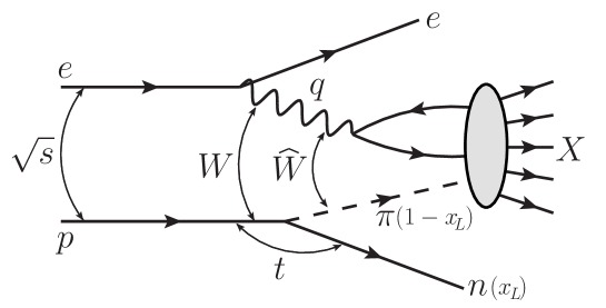
Figure 1: Leading neutron $n$ production in $ep\rightarrow enX$ interactions at high energies. $x_{L}$ is momentum fraction of the proton carried by the neutron $n$.

II Leading neutron production in the color dipole formalism

II.1 The cross section

Let us review the main formulas of leading neutron production. At high energies, this scattering can be seen as a set of three factorizable subprocesses (See Fig. 1): i) the photon fluctuates into a quark-antiquark pair (the color dipole), ii) the color dipole interacts with the pion, present in the wave function of the incident proton, and iii) the leading neutron is formed. The differential cross section reads:

$$\frac{d^{2}\sigma(W,Q^{2},x_{L},t)}{dx_{L}dt}=f_{\pi/p}(x_{L},t)\sigma_{\gamma^{*}\pi}(\hat{W}^{2},Q^{2})$$ (1)

where $Q^{2}$ is the virtuality of the exchanged photon, $\hat{W}$ is the center-of-mass energy of the virtual photon-pion system. It can be written as $\hat{W}^{2}=(1-x_{L})\,W^{2}$, where $W$ is the center-of-mass energy of the virtual photon-proton system. As it can be seen in Fig. 1, $x_{L}$ is the proton momentum fraction carried by the neutron and $t$ is the square of the four-momentum of the exchanged pion. In terms of the measured quantities $x_{L}$ and transverse momentum $p_{T}$, the pion virtuality is:

$$t\simeq-\frac{p_{T}^{2}}{x_{L}}-\frac{(1-x_{L})(m_{n}^{2}-m_{p}^{2}x_{L})}{x_{L}}$$ (2)

The flux of virtual pions emitted by the proton is represented by $f_{\pi/p}$ and $\sigma_{\gamma^{*}\pi}(\hat{W}^{2},Q^{2})$ is the cross section for the interaction between the virtual-photon and the virtual-pion at center-of-mass energy $\hat{W}$.

II.2 The pion flux

The pion flux $f_{\pi/p}(x_{L},t)$ (also called sometimes pion splitting function) is the virtual pion momentum distribution in a physical nucleon (the bare nucleon plus the “pion cloud”). It was first calculated in the early studies sullivan of deep inelastic scattering (DIS), where a pseudoscalar nucleon-pion-nucleon vertex was added to the standard DIS diagram. These early calculations were further refined in Refs. cloud and even extended to the strange and charm sector charm . Since pion emission is a nonperturbative process, once we depart from the single nucleon state, we should consider a whole tower of meson-baryon states, having to deal with a series for which there is no rigorous truncation scheme. This led some authors to use light cone models ma for the pion momentum distribution, where the dynamical origin of the pion is not mentioned and one tries to determine phenomenologically the relative weight of the higher Fock states.

In all the calculations of the pion flux a form factor was introduced to represent the non pointlike nature of hadrons and hadronic vertices, which contain a cut-off parameter determined by fitting data. The most frequently used parametrizations of the pion flux holt ; bisha ; kope ; kuma ; niko99 ; models ; kkmr ; khoze ; speth ; pirner have the following general form:

$$f_{\pi/p}(x_{L},t)=\frac{1}{4\pi}\frac{2g_{p\pi p}^{2}}{4\pi}\frac{-t}{(t-m_{\pi}^{2})^{2}}(1-x_{L})^{1-2\alpha(t)}[F(x_{L},t)]^{2}$$ (3)

where $g_{p\pi p}^{2}/(4\pi)=14.4$ is the $\pi^{0}pp$ coupling constant, $m_{\pi}$ is the pion mass and $\alpha(t)$ will be defined below. The form factor $F(x_{L},t)$ accounts for the finite size of the nucleon and pion. We will consider the following parametrizations of the form factor:

$$F_{1}(x_{L},t)=\exp\left[R^{2}\frac{(t-m_{\pi}^{2})}{(1-x_{L})}\right]\,\,\,\,,\,\,\,\,\alpha(t)=0$$ (4)

from Ref. holt , where $R=0.6$ GeV^-1.

$$F_{2}(x_{L},t)=1\,\,\,\,,\,\,\,\,\alpha(t)=\alpha(t)_{\pi}$$ (5)

from Ref. bisha , where $\alpha_{\pi}(t)\simeq t$ (with $t$ in GeV²) is the Regge trajectory of the pion.

$$F_{3}(x_{L},t)=\exp\left[b(t-m_{\pi}^{2})\right]\,\,\,\,,\,\,\,\,\alpha(t)=\alpha(t)_{\pi}$$ (6)

from Ref. kope , where $b=0.3$ GeV^-2.

$$F_{4}(x_{L},t)=\frac{\Lambda_{m}^{2}-m_{\pi}^{2}}{\Lambda_{m}^{2}-t}\,\,\,\,,\,\,\,\,\alpha(t)=0$$ (7)

from Ref. kuma , where $\Lambda_{m}=0.74$ GeV.

$$F_{5}(x_{L},t)=\left[\frac{\Lambda_{d}^{2}-m_{\pi}^{2}}{\Lambda_{d}^{2}-t}\right]^{2}\,\,\,\,,\,\,\,\,\alpha(t)=0$$ (8)

also from Ref. kuma , where $\Lambda_{d}=1.2$ GeV. In the case of the more familiar exponential (4), monopole (7) and dipole (8) forms factors, the cut-off parameters have been determined by fitting low energy data on nucleon and nuclear reactions and also data on deep inelastic scattering and structure functions.

In all analyses of pion cloud effects in DIS the authors have used pseudoscalar (PS) coupling, which is, by itself, inconsistent with chiral symmetry. More recently, in wally the authors used an effective chiral Lagrangian for the interaction of pions and nucleons consistent with chiral symmetry. Unlike the earlier chiral effective theory calculations which only computed the light-cone distributions of pions or considered the non analytic behaviour of their moments to lowest order in the pion mass, in wally the authors have computed the complete set of diagrams relevant for DIS from nucleons dressed by pions resulting from their Lagrangians, without taking the heavy baryon limit. In particular, they have demonstrated explicitly the consistency of the computed distribution functions with electromagnetic gauge invariance. In wally2 they applied the previously computed pion distribution to the study of the $\bar{d}-\bar{u}$ asymmetry in the nucleon. For our purposes, the relevant contribution of the pion momentum distribution reads wally :

$$f_{\pi/p}(y)=\frac{g_{A}^{2}m_{n}^{2}}{(4\pi f_{\pi})^{2}}\int_{0}^{\Lambda_{c}^{2}}dp_{T}^{2}\frac{y(p_{T}^{2}+y^{2}m_{n}^{2})}{[p_{T}^{2}+y^{2}m_{n}^{2}+(1-y)m_{\pi}^{2}]^{2}}$$ (9)

where $y=1-x_{L}$, $g_{A}=1.267$ is the nucleon axial charge, $f_{\pi}=93$ MeV and $\Lambda_{c}=0.2$ GeV. In order to obtain the final cross section we multiply (9) by 2 (see wally ; wally2 ) and insert it into (1) after integrating the latter over $t$ (or over $p_{T}$).

In what follows, we shall use the pion fluxes listed above, in equations (4)-(9), denoting them by $f_{1}$, $f_{2}$, … $f_{6}$, respectively. The main purpose of our calculation will be to show that the dipole approach gives a good description of data and the pion flux is just one element of the calculation. Therefore we will make no effort to choose one particular form. Nevertheless, we note that one important phenomenological constraint that these pion fluxes must satisfy is to reproduce the $\bar{d}-\bar{u}$ asymmetry in the proton sea measured by the E866 Collaboration e866 . Among the pion fluxes mentioned above only (8) (see babi00 ) and (9) have been confronted with these data. As it will be seen later, the results discussed here are very sensitive to the choice of the pion flux and hence leading neutron spectra may be used to constrain its shape.

Before closing this subsection we would like to mention that the diagram shown in Fig.1 represents only the dominant contribution to leading neutron production. Other isovector meson exchanges, such as $\rho$ or $a_{2}$, can also contribute to the leading neutron spectrum. Moreover the $p\rightarrow\Delta$ transition can also contribute to neutron production through the subsequent decay $\Delta\rightarrow n\pi$. Theoretical studies show that processes other than direct pion exchange are expected to give a contribution of less than $25$ % of the cross section holt ; kope ; kuma ; niko99 ; iso . The effect of these backgrounds to the one pion exchange is to increase the rate of neutron production. However this effect is partially compensated by the absorptive rescattering of the neutron, which decreases the neutron rate by approximately the same amount speth ; pirner .

II.3 The photon-pion cross section

In order to obtain the photon-pion cross section we will use the color dipole formalism, as usually done in high energy deep inelastic scattering off a nucleon target. In this formalism, the cross section is factorized in terms of the photon wave functions $\Psi$, which describes the photon splitting in a $q\bar{q}$ pair, and the dipole-pion cross section $\sigma_{d\pi}$. We have

$$\sigma_{\gamma^{*}\pi}(\hat{x},Q^{2})=\int_{0}^{1}dz\int d^{2}\mbox{\boldmath$r$}\sum_{L,T}\left|\Psi_{T,L}(z,\mbox{\boldmath$r$},Q^{2})\right|^{2}\sigma_{d\pi}(\hat{x},\mbox{\boldmath$r$})$$ (10)

where

$$\hat{x}=\frac{Q^{2}+m^{2}_{f}}{\hat{W}^{2}+Q^{2}}=\frac{Q^{2}+m^{2}_{f}}{(1-x_{L})W^{2}+Q^{2}}$$ (11)

is the scaled Bjorken variable and the variable $r$ defines the relative transverse separation of the pair (dipole). Moreover, we have that the photon wave functions are given by

$$\left|\psi_{L}(z,\mbox{\boldmath$r$})\right|^{2} = \frac{3\alpha_{em}}{2\pi^{2}}\sum_{f}e_{f}^{2}4Q^{2}z^{2}(1-z)^{2}K_{0}^{2}(\epsilon r)$$ (12)

$$\left|\psi_{T}(z,\mbox{\boldmath$r$})\right|^{2} = \frac{3\alpha_{em}}{2\pi^{2}}\sum_{f}e_{f}^{2}\left\{[z^{2}+(1-z)^{2}]\epsilon^{2}K_{1}^{2}(\epsilon r)+m_{f}^{2}K_{0}^{2}(\epsilon r)\right\}$$ (13)

for a longitudinally (L) and transversely (T) polarized photon, respectively. In the above expressions $\epsilon^{2}=z(1-z)Q^{2}+m_{f}^{2}\;,$ $K_{0}$ and $K_{1}$ are modified Bessel functions and the sum is over quarks of flavour $f$ with a corresponding quark mass $m_{f}$. As usual $z$ stands for the longitudinal photon momentum fraction carried by the quark and $1-z$ is the longitudinal photon momentum fraction of the antiquark.

The main input in the calculations of $\sigma_{\gamma^{*}\pi}$ is the dipole-pion cross section. In what follows, for simplicity, we will assume the validity of the additive quark model, which allows us to relate $\sigma_{d\pi}$ with the dipole-proton cross section, usually probed in the typical inclusive and exclusive processes at HERA. Basically, we will assume that

$$\sigma_{d\pi}({x},\mbox{\boldmath$r$})=\frac{2}{3}\cdot\sigma_{dp}({x},\mbox{\boldmath$r$})$$ (14)

This is assumption is supported by the study of the pion structure function in the low x regime presented in zoller . It also gives a good description of the previous ZEUS leading neutron spectra, as shown in kkmr ; khoze . On the other hand, the direct application of (1) to HERA photoproduction data zeus02 leads to the result $\sigma^{\mbox{tot}}_{\gamma\pi}/\sigma^{\mbox{tot}}_{\gamma p}=0.32\pm 0.03$, which is factor 2 lower than the ratio given above. This subject certainly deserves more detailed studies in the future. For our purposes, the use of relation (14) allows us to estimate $\sigma_{d\pi}$ without additional free parameters. In the eikonal approximation the dipole-proton cross section $\sigma_{dp}$ is given by:

$$\sigma_{dp}(x,\mbox{\boldmath$r$})=2\int d^{2}\mbox{\boldmath$b$}\,{\cal N}^{p}(x,\mbox{\boldmath$r$},\mbox{\boldmath$b$})\,\,,$$ (15)

where $\mathcal{N}^{p}(x,\mbox{\boldmath$r$},\mbox{\boldmath$b$})$ is the imaginary part of the forward amplitude for the scattering between a small dipole (a colorless quark-antiquark pair) and a dense hadron target, at a given rapidity interval $Y=\ln(1/x)$. The dipole has transverse size given by the vector $\mbox{\boldmath$r$}=\mbox{\boldmath$x$}-\mbox{\boldmath$y$}$, where $x$ and $y$ are the transverse vectors for the quark and antiquark, respectively, and impact parameter $\mbox{\boldmath$b$}=(\mbox{\boldmath$x$}+\mbox{\boldmath$y$})/2$. As mentioned in the introduction, at very high energies (and very low $x$) the evolution with the rapidity $Y$ of $\mathcal{N}^{p}(x,\mbox{\boldmath$r$},\mbox{\boldmath$b$})$ is given by the Balitsky-Kovchegov (BK) equation BAL ; kov assuming the translational invariance approximation, which implies $\mathcal{N}^{p}(x,\mbox{\boldmath$r$},\mbox{\boldmath$b$})=\mathcal{N}^{p}(x,\mbox{\boldmath$r$})S(\mbox{\boldmath$b$})$ and $\sigma_{dp}(x,\mbox{\boldmath$r$})=\sigma_{0}\cdot{\cal N}^{p}(x,\mbox{\boldmath$r$})$, with the normalization of the dipole cross section ($\sigma_{0}$) being fitted to data. Alternatively, we can describe the scattering amplitude $\mathcal{N}^{p}(x,\mbox{\boldmath$r$})$ using phenomenological models based on saturation physics constructed taking into account the analytical solutions of the BK equation which are known in the low and high density regimes. The main advantage in the use of phenomenological models is that we can easily to compare the linear and nonlinear predictions, which is useful to determine the contribution of the saturation effects for the process under analysis. In what follows we will consider as input the phenomenological models proposed in Refs. GBW ; iim ; soyez . In particular, the IIMS model, proposed in Ref. iim and updated in soyez , was constructed so as to reproduce two limits of the LO BK equation analytically under control: the solution of the BFKL equation for small dipole sizes, $r\ll 1/Q_{s}(x)$, and the Levin-Tuchin law for larger ones, $r\gg 1/Q_{s}(x)$. In the updated version of this parametrization soyez , the free parameters were obtained by fitting the new H1 and ZEUS data. In this parametrization the forward dipole-proton scattering amplitude is given by

$${\cal{N}}^{p}(x,\mbox{\boldmath$r$})=\left\{\begin{array}[]{ll}{\mathcal{N}}_{0}\,\left(\frac{r\,Q_{s}}{2}\right)^{2\left(\gamma_{s}+\frac{\ln(2/r\,Q_{s})}{\kappa\,\lambda\,Y}\right)}\,,&\mbox{for $rQ_{s}({x})\leq 2$}\,,\\ 1-\text{e}^{-a\,\ln^{2}\,(b\,r\,Q_{s})}\,,&\mbox{for $rQ_{s}({x})>2$}\,,\end{array}\right.$$ (18)

where $a$ and $b$ are determined by continuity conditions at $rQ_{s}({x})=2$, $\gamma_{s}=0.7376$, $\kappa=9.9$, ${\mathcal{N}}_{0}=0.7$ and $Q_{s}$ is the saturation scale given by:

$$Q^{2}_{s}({x})=Q^{2}_{0}\left(\frac{x_{0}}{{x}}\right)^{\lambda}$$ (19)

with $x_{0}=1.632\times 10^{-5}$, $\lambda=0.2197$, $Q_{0}^{2}=1.0$ GeV². The first line of Eq. (18) describes the linear regime whereas the second one includes saturation effects. On the other hand, in the GBW model GBW , the dipole-proton scattering amplitude is given by

$${\cal{N}}^{p}(x,\mbox{\boldmath$r$})=1-\exp\left[-\frac{Q_{s}^{2}r^{2}}{4}\right]$$ (20)

with $Q_{0}^{2}=1.0$ GeV², $x_{0}=3\times 10^{-4}$ and $\lambda=0.288$. Finally, we will also use the dipole-proton cross section estimated with the help of the DGLAP analysis of the gluon distribution, which is given by predazzi :

$$\sigma_{dip}(x,\mbox{\boldmath$r$})=\frac{\pi^{2}}{3}r^{2}\alpha_{s}{x}g(x,10/r^{2})$$ (21)

where $xg(x,Q^{2})$ is the target gluon distribution, for which we use the CTEQ6 parametrization lai . The above expression represents the linear regime of QCD and is a baseline for comparison with the nonlinear predictions.

III Results

As it was seen in the previous sections, the leading neutron spectrum depends essentially on two main ingredients: the pion flux and the dipole-pion cross section. The latter is very sensitive to the value of the involved Bjorken $x$, or, in our case, $\hat{x}$. In Fig. 2 we show $\hat{x}$ as a function of $x_{L}$. From the figure we can conclude that at the highest values of the present photon-hadron energies ($W$) and at the lowest values of $Q^{2}$ we enter deeply in the low $x$ domain. This will be even more so if measurements can be carried out at higher energies, but already at the available energies we can see that the leading neutron spectrum receives a contribution from the kinematical range where the nonlinear effects are expected to be present and hence it is interesting to investigate their influence.

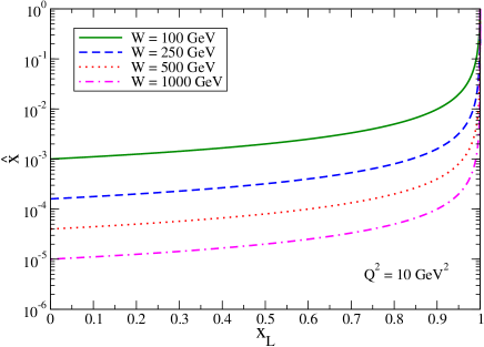
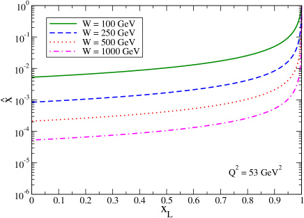
(a)		(b)

Figure 2: Scaled Bjorken variable $\hat{x}$, (Eq. 11), as a function of $x_{L}$ for two different virtualities: (a) $Q^{2}=10$ GeV² and (b) $Q^{2}=53$ GeV².

We address now the dependence of our predictions for the leading neutron spectra on the models of the pion flux and of the dipole-pion scattering amplitude. It is important to emphasize that the spectrum is proportional to the product of these two quantities. Consequently, in what follows we will initially assume a given model for one of these quantities and analyse the dependence on the other quantity. Having done that, we will choose one combination, calculate the normalized cross section $(1/\sigma_{DIS})d\sigma/dx_{L}$ and compare with the experimental data. The normalization was taken from Ref. snorm and is given by:

$$\sigma_{DIS}=\frac{4\pi^{2}\alpha_{em}}{Q^{2}}\frac{c}{x^{\beta}}$$ (22)

where $c=0.18$, $\beta=d\,\ln(Q^{2}/\Lambda_{0}^{2})$ with $d=0.0481$ and $\Lambda_{0}=0.292$ GeV. In Fig. 3 (a) we consider the IIMS model for the scattering amplitude and estimate the leading neutron spectrum using the different models of the pion flux discussed in the previous section. We observe that the behavior at medium and small values of $x_{L}$ is strongly dependent on the choice of the model. Using the cut-off $\Lambda_{c}$ in the range defined in Ref. wally2 , our results suggest that model $f_{6}$ is disfavored. In Fig. 3 (b) we consider the $f_{2}$ model for the pion flux and estimate the spectra using different models of the scattering amplitude. We can see that the predictions have similar behavior in the transition between the small and large-$x_{L}$ regimes, but with the magnitude being dependent on the description of the QCD dynamics. In the previous analysis we have considered $Q^{2}=53$ GeV². However, the experimental data were obtained for a wide range of virtualities, which implies that there is some arbitrariness present in the choice of the value of $Q^{2}$ used in our calculations. In order to estimate the uncertainty present in this choice, in Fig. 3 (c) we consider the $f_{2}$ and IIMS models and calculate the spectrum for different values of the photon virtuality. We observe that our predictions are more compatible with the experimental data if larger values of $Q^{2}$ are assumed.

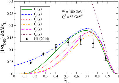
(a)

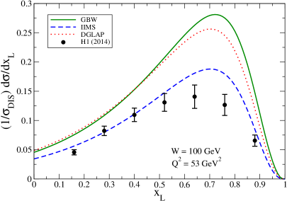
(b)

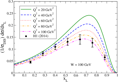
(c)

Figure 3: Leading neutron spectra compared with experimental data at $W=100$ GeV considering (a) the IIMS scattering amplitude and different choices of the pion flux ($Q^{2}=53$ GeV²); (b) the $f_{2}$ pion flux and different choices for the scattering amplitude ($Q^{2}=53$ GeV²); and (c) the $f_{2}$ pion flux and the IIMS scattering amplitude for different values of photon virtuality $Q^{2}$.

So far we have assumed that the photon hits only the pion, in a type of “impulse aproximation”. However it has been shown in pirner that very often the photon hits also the neutron, specially in the low $Q^{2}$ domain, where the photon has low resolving power. In these cases the extra interactions generate the so called absorptive corrections, which can be estimated with models. In the case of leading neutron production, it has been shown pirner that the corrections are not very large and affect almost uniformly all the $x_{L}$ spectrum. Using the results of pirner , we shall here simply multiply our spectra by the absorptive correction factor, $K_{abs}=0.7$.

In Fig. 4 we give our description of data, which is quite reasonable. All the parameters contained in the dipole cross section have been already fixed by the analysis of other DIS data from HERA. The pion flux has been fixed by fitting data of low energy hadronic collisions. As metioned above, it has been argued that the factor $\frac{2}{3}$ predicted by the additive quark model to relate the photon-pion and photon-proton cross sections could be smaller, closer to $\frac{1}{3}$. Using this different factor, we would then underpredict the data in the low $x_{L}$ region. In principle, this would be acceptable since in this region other processes are expected to play a role. As already emphasized, this subject deserves more detailed studies.

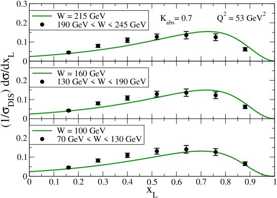
Figure 4: Leading neutron $x_{L}$ spectrum for three photon-proton energies compared with recent H1 data.

Finally, we analyse the Feynman scaling in the leading neutron spectra and the contribution of nonlinear effects for this process. As mentioned before this process is surprisingly sensitive to low $x$ physics. In particular, the large $x_{L}$ ($x_{L}>0.3$) we observe the transition from the large to small $x$ domain. It is therefore interesting to check whether gluon saturation effects are already playing a significant role. As it can be seen from Eqs. (1) and (10), all the energy dependence is contained in the dipole forward scattering amplitude $\cal{N}$. Therefore, we can estimate the contribution of the nonlinear effects comparing the results obtained with saturation model, e.g. the IIMS model given in (18), with those obtained with the linear model, Eq. (21). Moreover, the theoretical expectation can be obtained using the GBW model for the scattering amplitude, Eq. (20). In the linear limit, when the dipole radius is very small (or equivalently $Q^{2}$ is very large) or the saturation scale is very small (and hence the energy is not very high), we can expand the exponent and obtain

$$\sigma_{d\pi}(r,\hat{x})\propto\sigma_{0}\,{\cal{N}}(r,\hat{x})\simeq\sigma_{0}\,\frac{Q^{2}_{s}(\hat{x})r^{2}}{4}\simeq\sigma_{0}\,Q^{2}_{0}\,{x_{0}}^{\lambda}\left[\frac{(1-x_{L})W^{2}+Q^{2}}{Q^{2}+m^{2}_{f}}\right]^{\lambda}\,\,.$$ (23)

Consequently, in this regime we see that the leading neutron $x_{L}$ spectrum will depend on $W$. In a complementary way, in the nonlinear limit, when the dipole radius is very large (or equivalently $Q^{2}$ is very small) or the saturation scale is very large (and hence the energy is very high), we obtain

$$\sigma_{d\pi}(r,\hat{x})\propto\sigma_{0}\,{\cal{N}}(r,\hat{x})\simeq\sigma_{0}\$$ (24)

which is energy independent. One could argue that the mere inspection of Eq. (1) would suggest that at some asymptotically high energy the photon-pion cross section would reach some “black disk” limit and the energy dependence would disappear. We would like to emphasize that the information contained in (23) and (24) is much richer and indicates the route through which the asymptotic limit is reached and the role played by nonlinear effects. These expectations can be compared with those obtained using the IIMS and DGLAP models for the dipole-pion cross section. In Fig. 5 (a) we show the spectra obtained in a purely linear approach. As expected we see a noticeable energy dependence. In contrast, the nonlinear predictions presented in Fig. 5 (b) show a remarkable suppression of the energy dependence at low values of $Q^{2}$, consistent with the expectations. These results indicate that the Feynman scaling (and how it is violated) can be directly related to the QCD dynamics at small-$x$.

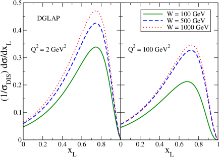
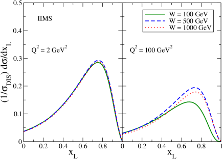
(a)		(b)

Figure 5: (a) Leading neutron spectra for different energies considering (a) the linear DGLAP model and (b) the nonlinear IIMS model for the dipole-pion cross section.

IV Summary

In this work we have studied leading neutron production in $e+p\rightarrow e+n+X$ collisions at high energies and have calculated the Feynman $x_{L}$ distribution of these neutrons. The differential cross section was written in terms of the pion flux and the photon-pion total cross section. We have proposed to describe this process using the color dipole formalism and, assuming the validity of the additive quark model, we have related the dipole-pion with the well determined dipole-proton cross section. In this formalism we have been able to estimate the dependence of the predictions on the description of the QCD dynamics at high energies as well as the contribution of the gluon saturation effects for the leading neutron production. With the parameters strongly constrained by other phenomenological information, we were able to reproduce the recently released H1 leading neutron spectra. One of our most interesting conclusions is that leading neutron spectra can be used to probe the low $x$ content of the pion target and hence it is a new observable where we can look for gluon saturation effects. At higher energies this statement will become more valid. Moreover saturation physics provides a precise route to Feynman scaling, which will eventually happen at higher energies. These conclusions motivate more detailed studies, in particular in the subjects which are the main source of theoretical uncertainties in our calculations: i) the validity of the additive quark model; ii) the factor $K_{abs}$ accounting for the absorptive corrections, which are model dependent; iii) the precise form of the pion flux; iv) the precise form of the dipole cross section. It is important to emphasize that none of these numbers or functions is free. On the contrary, they are subject to severe constraints from other experimental information and the freedom to choose them will be further reduced in the future.

- (1) D.S. Barton et al., Phys. Rev. D 27, 2580 (1982); A.E. Brenner et al., Phys. Rev. D 26, 1497 ( 1982); EHS/NA22 Collaboration, N.M. Agababyan et al., Z. Phys. C 75, 229 (1996); N. Cartiglia, AIP Conf. Proc. 407, 515 (1997); S. Chekanov et al. [ZEUS Collaboration], Phys. Lett. B 590, 143 (2004). S. Chekanov et al. [ZEUS Collaboration], Nucl. Phys. B 776, 1 (2007).
- (2) J. Olsson [H1 Collaboration], PoS DIS 2014, 156 (2014); V. Andreev et al. [H1 Collaboration], Eur. Phys. J. C 74, 2915 (2014); F. D. Aaron et al. [H1 Collaboration], Eur. Phys. J. C 68, 381 (2010).
- (3) M. Bishari, Phys. Lett. B 38, 510 (1972).
- (4) H. Holtmann et al., Phys. Lett. B 338, 363 (1994).
- (5) B. Kopeliovich, B. Povh and I. Potashnikova, Z. Phys. C 73, 125 (1996).
- (6) S. Kumano, Phys. Rev. D 43, 59 (1991).
- (7) N.N. Nikolaev et al., Phys. Rev. D 60, 014004 (1999).
- (8) L.L. Frankfurt, L. Mankiewicz and M.I. Strikman, Z. Phys. A 334, 343 (1989); T.T. Chou and C.N. Yang, Phys. Rev. D 50, 590 (1994); K. Golec-Biernat, J. Kwiecinski and A. Szczurek, Phys. Rev. D 56, 3955 (1997); M. Przybycien, A. Szczurek and G. Ingelman, Z. Phys. C 74, 509 (1997); W. Melnitchouk, J. Speth and A.W. Thomas, Phys. Rev. D 59, 014033 (1998); A. Szczurek, N.N. Nikolaev and J. Speth, Phys. Lett. B 428, 383 (1998).
- (9) A.B. Kaidalov,V.A. Khoze, A.D. Martin and M.G. Ryskin, Eur. Phys. J. C 47, 385 (2006).
- (10) V.A. Khoze, A.D. Martin and M.G. Ryskin, Eur. Phys. J. C 48, 797 (2006).
- (11) N.N. Nikolaev, J. Speth and B.G. Zakharov, hep-ph/9708290.
- (12) U. DAlesio and H.J. Pirner, Eur. Phys. J. A 7, 109 (2000).
- (13) See, for example, ZEUS Collaboration, M. Derrick et al., Phys. Lett. B 384, 388 (1996).
- (14) M. Burkardt, K. S. Hendricks, C. R. Ji, W. Melnitchouk and A. W. Thomas, Phys. Rev. D 87, 056009 (2013).
- (15) Y. Salamu, C. R. Ji, W. Melnitchouk and P. Wang, Phys. Rev. Lett. 114, 122001 (2015).
- (16) F. Gelis, E. Iancu, J. Jalilian-Marian and R. Venugopalan, Ann. Rev. Nucl. Part. Sci. 60, 463 (2010);E. Iancu and R. Venugopalan, arXiv:hep-ph/0303204; H. Weigert, Prog. Part. Nucl. Phys. 55, 461 (2005); J. Jalilian-Marian and Y. V. Kovchegov, Prog. Part. Nucl. Phys. 56, 104 (2006); J. L. Albacete and C. Marquet, Prog. Part. Nucl. Phys. 76, 1 (2014).
- (17) J. Jalilian-Marian, A. Kovner, L. McLerran and H. Weigert, Phys. Rev. D 55, 5414 (1997); J. Jalilian-Marian, A. Kovner and H. Weigert, Phys. Rev. D 59, 014014 (1999), ibid. 59, 014015 (1999), ibid. 59 034007 (1999); A. Kovner, J. Guilherme Milhano and H. Weigert, Phys. Rev. D 62, 114005 (2000); H. Weigert, Nucl. Phys. A703, 823 (2002); E. Iancu, A. Leonidov and L. McLerran, Nucl.Phys. A692, 583 (2001); E. Ferreiro, E. Iancu, A. Leonidov and L. McLerran, Nucl. Phys. A701, 489 (2002).
- (18) I. I. Balitsky, Phys. Rev. Lett. 81, 2024 (1998); Phys. Lett. B 518, 235 (2001); I.I. Balitsky and A.V. Belitsky, Nucl. Phys. B 629, 290 (2002).
- (19) Y.V. Kovchegov, Phys. Rev. D 60, 034008 (1999); Phys. Rev. D 61 074018 (2000).
- (20) T. Sako [LHCf Collaboration], arXiv:1010.0195 [hep-ex].
- (21) O. Adriani, L. Bonechi, M. Bongi, G. Castellini, R. D’Alessandro, A. Faus, K. Fukatsu and M. Haguenauer et al., Nucl. Phys. Proc. Suppl. 212, 270 (2011).
- (22) Y. Itow, H. Menjo, G. Mitsuka, T. Sako, K. Kasahara, T. Suzuki, S. Torii and O. Adriani et al., arXiv:1401.1004 [physics.ins-det]; Y. Itow, H. Menjo, T. Sako, N. Sakurai, K. Kasahara, T. Suzuki, S. Torii and O. Adriani et al., arXiv:1409.4860 [physics.ins-det]; L. Bonechi, O. Adriani, E. Berti, M. Bongi, G. Castellini, R. D’Alessandro, M. Del Prete and M. Haguenauer et al., EPJ Web Conf. 71, 00019 (2014).
- (23) J.D. Sullivan, Phys. Rev. D 5, 1732 (1972); A.W. Thomas, Phys. Lett. B 126, 97 (1983).
- (24) W. Melnitchouk and M. Malheiro, Phys. Rev. C 55, 431 (1997); J. Speth and A. W. Thomas, Adv. Nucl. Phys. 24, 83 (1998); S. Kumano, Phys. Rep. 303, 183 (1998); H. Holtmann, A. Szczurek and J. Speth, Nucl. Phys. A 569, 631 (1996); N.N. Nikolaev, W. Schaefer, A. Szczurek and J. Speth, Phys. Rev. D 60, 014004 (1999).
- (25) F. S. Navarra, M. Nielsen, C. A. A. Nunes and M. Teixeira, Phys. Rev. D 54, 842 (1996); S. Paiva, M. Nielsen, F. S. Navarra, F. O. Durães and L. L. Barz, Mod. Phys. Lett. A 13, 2715 (1998); W. Melnitchouk and A.W. Thomas, Phys. Lett. B 414, 134 (1997).
- (26) S. J. Brodsky and B. Q. Ma, Phys. Lett. B 381, 317 (1996).
- (27) E. A. Hawker et al., E866/NuSea Collaboration, Phys. Rev. Lett. 80, 3715 (1998).
- (28) F. Carvalho, F. O. Duraes, F. S. Navarra, M. Nielsen and F. M. Steffens, Eur. Phys. J. C 18, 127 (2000).
- (29) A. W. Thomas and C. Boros, Eur. Phys. J. C 9, 267 (1999);
- (30) N.N. Nikolaev, J. Speth and V.R. Zoller, Phys. Lett. B 473, 157 (2000).
- (31) S. Chekanov et al. [ZEUS Collaboration], Nucl. Phys. B 637, 3 (2002).
- (32) K. J. Golec-Biernat, M. Wusthoff, Phys. Rev. D 59, 014017 (1998).
- (33) E. Iancu, K. Itakura, S. Munier, Phys. Lett. B 590, 199 (2004).
- (34) G. Soyez, Phys. Lett. B 655, 32 (2007).
- (35) V. Barone and E. Predazzi, High-Energy Particle Diffraction, Springer-Verlag, Berlin Heidelberg, (2002); E. Iancu and A. H. Mueller, Nucl. Phys. A 730, 460 (2004); G. P. Salam, Nucl. Phys. B 461, 512 (1996).
- (36) H. L. Lai, J. Huston, Z. Li, P. Nadolsky, J. Pumplin, D. Stump and C.-P. Yuan, Phys. Rev. D 82, 054021 (2010).
- (37) C. Adloff et al., Phys. Lett. B 520, 183 (2001).