Abstract

Abstract. We suggest a novel shape matching algorithm for three-dimensional surface meshes of disk or sphere topology. The method is based on the physical theory of nonlinear elasticity and can hence handle large rotations and deformations. Deformation boundary conditions that supplement the underlying equations are usually unknown. Given an initial guess, these are optimized such that the mechanical boundary forces that are responsible for the deformation are of a simple nature. We show a heuristic way to approximate the nonlinear optimization problem by a sequence of convex problems using finite elements. The deformation cost, i.e., the forces, is measured on a coarse scale while ICP-like matching is done on the fine scale. We demonstrate the plausibility of our algorithm on examples taken from different datasets.

1 Introduction

1.1 Motivation

Shape matching is a difficult but nonetheless important problem in computer vision, medical imaging, and computer graphics. It is the key ingredient for recognition, retrieval, alignment of scanned data, information transfer, shape interpolation, statistical shape modeling, space-time reconstruction and more.

This work aims to contribute a novel framework to solve for unknown shape deformations of a pair of two-dimensional surfaces (source and target) in three dimensions. Our method is built on the observation that in applications surfaces often represent the boundaries of actual physical entities, i.e., surfaces of elastic bodies. Shape change can therefore be explained by means of forces acting on the specific elastic body. Their magnitude can be interpreted as a measure of how “difficult” it is to achieve a certain shape change. Elastic models are, we believe, well suited to give valuable information about shape changes among different objects. In particular, we believe, that sparsity of forces is a good prior for explaining an observed deformation within a semantic class of objects, e.g., if we were to compare two different shape articulations.

From a mathematical point of view shape matching is an ill-posed inverse problem and is usually tackled in a heuristic manner. It is computationally challenging since the search space for correspondences is usually large. Hence, there is a need to explore this search space in a reasonable manner.

1.2 Our Method

In [45] the authors intuitively describe the desired shape blending algorithm as one which requires the least work to deform through bending and stretching. Many shape matching algorithms are designed in this spirit as one usually seeks “maximum alignment by means of minimal cost” in an optimization framework. Our work uses the physical theory of nonlinear elasticity and is based on the same principle as will be elaborated in the following.

In this work we suggest a method for aligning two surface meshes (manifolds) embedded in three-dimensional space. We use the observation that surface meshes often represent (parts of) the boundaries of actual physical bodies. Hence, the cost of a deformation of a surface can be measured by forces acting on the boundary of the solid body described by the surface.

We believe that in many realistic scenarios even complicated deformations take place due to or can be explained by means of surprisingly simple forces. Examples are the change of a pose of an animal or a human where forces act mainly only on the articulated parts, i.e., the acting forces can be regarded as sparse. We furthermore anticipate that, given two semantically similar objects, seeking a deformation that is subject to sparse and isotropic surface forces is a reasonable strategy to match them. These forces could then be used to intuitively compare two different deformations and to assess their severity.

The underlying equations of nonlinear elasticity that we employ form a system of nonlinear partial differential equations (PDEs) and are subject to boundary conditions. These can be given as deformations and/or forces prescribed on the boundary of the body. Given two shapes boundary conditions of either type are usually unknown but one can often give an initial guess of boundary correspondences, i.e., of the boundary deformation. Such an initial guess can then be optimized according to our prior on the forces to obtain a “better” set of boundary correspondences that supplement the PDE. The initial guess plays the role of a spring force between source and target shape and a penalty needs to be paid for deviation. The optimized boundary correspondences can then be used to solve the underlying elasticity PDE using a common Newton-Raphson scheme to update the full volumetric deformation of the body and the entire procedure can be iterated until a good match is found.

Using the popular finite element method (FEM) we show how to connect the boundary deformation to the boundary forces by means of a splitting of the tangent stiffness matrix, localized around a certain deformation. This so-called condensation is necessary to reduce the optimization to the boundary of the body and has the advantage that it lowers the dimension of the optimization significantly. Furthermore, the condensation allows us to formulate the problem as a sequence of (convex) second order cone problems.

As elaborated above we aim to match surfaces represented by triangular meshes but the FEM works on volumetric meshes. Hence, we create a tetrahedral mesh of the body represented by the triangular mesh. The surface meshes that we match in our examples have between 9000 to 55000 triangles and constructing a tetrahedral mesh that resembles the surface density of meshes would result in a computationally very large problem. Therefore, we create a coarse tetrahedral approximation of the surface. Every point on the surface mesh can then be coupled to the coarse boundary mesh of the volumetric mesh. A deformation of the coarse boundary then induces a deformation of the surface. This way we can prescribe a matching (in particular the initial guess) on the surface mesh while measuring the deformation cost on the coarser volumetric mesh.

1.3 Previous Work

1.3.1 Overview

An optimization based shape matching algorithm usually consists of two ingredients. First, one needs a regularizer that determines (the preference of) the class of deformations in consideration. Well investigated is the field of rigid matching, i.e., the admissible transformations are translations and rotations [1, 25, 39]. This is a common scenario if one is given a range scan of rigid objects that can be aligned with a single rigid transform. For non-rigid matching common regularizers that are used in the literature are the popular As-Rigid-As-Possible (ARAP) functional [2] and the As-Affine-As-Possible (AAAP) functional [30, 33]. Both are often combined in one objective function. For a set of correspondences AAAP measures the deviation from a global affine transform and hence favors smooth deformations. ARAP locally measures the deviation from a rigid transform and is related to elasticity since it mimics mechanical stiffness. These methods work on tetrahedral meshes, i.e., they need volumetric meshes that represent the shape. In the context of surfaces recent ARAP-like methods have been introduced in [47, 32].

Elastically deformable models in graphics have been pioneered in the end of the 1980s in [50]. Generally speaking, these models use characterizing properties of geometric objects (curves, surface, volumes) to define functionals that penalize deviation from them. A curve in three dimensions, for example, is fully characterized (up to rigid motion) by two parameters, its curvature and its torsion and hence a motion of the curve that changes one of them is considered a deformation of the curve. For a volume it is the local isotropic change of lengths that characterizes a deformation (up to rigid motion). This principle is reflected in the physical theory of (nonlinear) elasticity [6, 18]. In the context of shape matching deformation models that borrow ideas from elasticity can be found in [23], where the authors use linear elasticity for the registration of three-dimensional medical images, as well as in [16] for fitting solid meshes to animated surfaces. In [17] a thin-plate spline regularizer is used for point matching. Non-linear elasticity is employed in [41] for medical imaging and in [43] where two-dimensional elasticity is employed for three-dimensional surface matching via mesh parametrization. However, there is a vast amount of (physical) deformation methods and we do not aim at discussing them in detail. An overview of methods used in graphics can be found in [38] and techniques used in vision and medical imaging in [27].

The second ingredient for a shape matching method is a data term that drives the deformation and/or describes dissimilarity between source and target shape. One way is to randomly sample candidate correspondences and to choose a deformation that best aligns the data. These RANSAC methods, which were first introduced in [24], are practical for low-dimensional mapping spaces. Recently they were extended to deal with deformation spaces of higher dimension [35].

Another popular group of methods comprises variants of the famous iterative closest point (ICP) algorithm, first introduced in [8, 15]. This iterative approach was first used for rigid matching and is well suited for various representations of geometric data. It is based on the computation of closest points between source and target. Since then efficient methods have been developed that use different sampling of correspondences, different weighting schemes that determine the confidence of a candidate match etc., see [39, 16, 30]. Recently, ICP has been applied as well in the context of non-rigid matching [3, 12, 14, 28]. Some of these papers deal with deformations of significant magnitude.

Techniques like multi-dimensional scaling (MDS) and generalized multi-dimensional scaling (GMDS) aim to find correspondences by regarding the shapes as Riemannian manifolds and try to find an embedding in a common metric space [12, 13]. Correspondences are then found in the common embedding space (which can even be a high-dimensional Riemannian manifold in the case of GMDS) rather than between the shapes themselves. This way ICP can be regarded as an instance of the Euclidean isometric matching problem. MDS and GMDS are elegant methods but computationally costly.

We note, however, that the vast literature and number of techniques can be classified also by other criteria. An excellent overview of the field and of classification criteria can be found in the survey paper [29].

1.3.2 Comparison

This work extends our work in [46] to three dimensions and large deformations. By favoring sparse forces as explanations for elastic deformations we use the same prior that we used in [46]. There we deal with small planar deformations. The forces there are invariant under infinitesimal rotations only, due to the use of linear elasticity and are, in particular, not invariant under general rotations.

In [16] the authors employ an enhanced version of linear elasticity by the use of rotation compensation, similar to co-rotated linear elasticity. This way they can deal with large rotations but this requires a large number of low dimensional singular value decompositions in each iteration, whereas we solely update the tangent stiffness matrix computed by the FEM. Another difference is that in our method the optimized boundary forces can be made rotation invariant once a matching deformation is found, and it is theoretically suitable for very large deformations.

The splitting of the tangent stiffness matrix that we employ to connect boundary forces and boundary displacements was previously used in [11] in the context of surgery simulation and in [46] for matching. The technique that we propose generalizes this idea to the nonlinear case and allows us to reduce the (nonlinear) matching problem to solving a sequence of convex problems that we formulate as second order cone problems while simultaneously reducing the computational complexity.

In our algorithm, the computational complexity, i.e., the degrees of freedom to be optimized, is furthermore reduced by measuring the deformation cost, i.e., the elastic forces, on a (coarse) tetrahedral mesh that is needed by the FEM. The corresponding deformation is then extended to the (fine) triangular surface mesh. Similar ideas have used in [30, 33, 48]. Furthermore, changing the coarseness of the tetrahedral mesh gives the user control over the computational complexity of the FEM part of the model while the coarseness of the surface mesh is fixed.

The matching and the computation of the initial guess is done on the fine scale of the surfaces. We project the source points onto the target favoring similar points (descriptor aided) during the first few iterations and then switch to Euclidean projection once a better alignment is reached. This way one can regard our method as a two-scale version of a non-rigid ICP-like algorithm since the matching is done on the fine scale while the cost, i.e., the boundary forces, is measured on the coarse scale of the volumetric mesh.

The paper is organized as follows. In Section 2 we give a concise overview of the model of a hyperelastic body and describe a nonlinear FEM that is used in the optimization procedure. The optimization is described in detail in Section 3. Experiments, implementation details and a description of the two-scale algorithm are given in Section 4. Section 5 concludes with a discussion.

2 Model and Numerical Methods

2.1 Hyperelasticity

The purpose of this section is to introduce the reader into the most important principles of nonlinear elasticity theory that are relevant in the sequel. As mentioned, our model optimizes elastic forces and hence it is important to understand what forces we refer to and how they act. Nonlinear elasticity is a well developed and complex field. Mathematically oriented introductions can be found in [6, 18, 10] and an engineering oriented introduction in [20].

Roughly speaking an elastic body is an open connected subset $\mathcal{B}\subset\mathbb{R}^{3}$ that reacts to applied forces with a deformation. It returns to its rest state (also called reference configuration) after the forces are removed and does not memorize previous deformations. The main equations of nonlinear elasticity describe a balance between the applied forces that cause the deformation and the internal force distribution inside the deformed body (stress) in the spirit of Newton’s second law. We will elaborate on this in the following.

Stress, Forces and Equilibrium. We assume that we are given an elastic body in its rest pose $\mathcal{B}\subset\mathbb{R}^{3}$, i.e., the rest pose is the volume that is occupied by the body when no forces are applied to it. A deformation of the body is described by a locally injective and smooth vector field $\Phi:\mathcal{B}\rightarrow\mathbb{R}^{3}$, i.e., any point $x\in\mathcal{B}$ in the reference configuration has a corresponding point $x^{\Phi}:=\Phi(x)\in\mathcal{B}^{\Phi}:=\Phi(\mathcal{B})$ in the deformed configuration. Any deformation should satisfy $\det(\nabla\Phi)>0$, i.e., subsets of $\mathcal{B}$ of positive measure are mapped to subsets of $\mathcal{B}^{\Phi}$ of positive measure.

Suppose now that the rest state $\mathcal{B}$ is subject to forces that describe the action of the outside world on it. These can either be volumetric forces $f^{\Phi}$, i.e., they are measured by per unit volume of the deformed configuration, or they can be surface forces $g^{\Phi}$ measured per unit surface area acting on $\partial\mathcal{B}^{\Phi}$. Examples for volumetric forces are gravity or electric field forces, whereas examples for surface forces are pressure or spring forces. The resulting deformation $\Phi$ induces an internal force distribution $t^{\Phi}:\mathcal{B}^{\Phi}\times\mathbb{S}^{2}\rightarrow\mathbb{R}^{3}$ inside $\mathcal{B}^{\Phi}$ that balances the external forces, the so-called Cauchy traction vector. This vector field depends on two arguments since it measures the force per unit area acting through any cross section of $\mathcal{B}^{\Phi}$ described by its unit normal $n^{\Phi}\in\mathbb{S}^{2}$ at $x^{\Phi}\in\mathcal{B}^{\Phi}$. This can be expressed through a linear relation $t(x^{\Phi},n^{\Phi})=T^{\Phi}(x^{\Phi})n^{\Phi}$ where $T^{\Phi}:\mathcal{B}^{\Phi}\rightarrow\mathbb{R}^{3\times 3}$ is the Cauchy stress tensor. Its rows represent the three tractions (normal and shear stresses) in three coordinate planes which are usually the three orthogonal canonical planes, see Figure 1 for an illustration. In particular, if $x^{\Phi}\in\partial\mathcal{B}^{\Phi}$ and $n^{\Phi}\in\mathbb{S}^{2}$ is its corresponding outward unit normal, then $t^{\Phi}(x^{\Phi},n^{\Phi})$ is the force $g^{\Phi}$ acting on the boundary of $\mathcal{B}^{\Phi}$ at this specific point. Boundary forces will be of importance in the sequel for the formulation of our optimization problem.

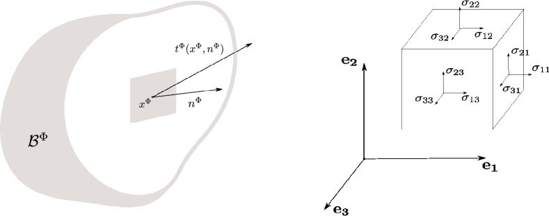
Figure 1: Left: an illustration of a surface force $t^{\Phi}(x^{\Phi},n^{\Phi})$ at some point $x^{\Phi}$ in an arbitrary cross section with normal $n^{\Phi}$ of a body $\mathcal{B}^{\Phi}$. Right: illustration of the three components of the Cauchy stress tensor $\sigma=T^{\Phi}$ with respect to the canonical coordinate planes. The normal stress is orthogonal to the considered plane shear stresses lie within the plane.

The basic equations governing elasticity theory can now be formulated as follows (Cauchy principle): Let the volumetric forces be denoted by $f^{\Phi}:\mathcal{B}^{\Phi}\rightarrow\mathbb{R}^{3}$ and let $\mathcal{V}\subset\mathcal{B}^{\Phi}$ be an arbitrary subvolume. Then

$$\int_{\partial\mathcal{V}}t^{\Phi}(x^{\Phi},n^{\Phi})\operatorname{d}S^{\Phi}+\int_{\mathcal{V}}f^{\Phi}(x^{\Phi})\operatorname{d}x^{\Phi}=0\>.$$ (1)

This equilibrium of external forces and internal stress is an expression of Newton’s second law and holds in the deformed configuration $\mathcal{B}^{\Phi}$. A similar principle for the angular moments shows in addition that $T^{\Phi}$ must be symmetric. Using the above and the divergence theorem we get

$$\int_{\mathcal{V}}\left(\operatorname{div}^{\Phi}T^{\Phi}(x^{\Phi})+f^{\Phi}(x^{\Phi})\right)\operatorname{d}x^{\Phi}=0\>.$$ (2)

Since this holds for all subvolumes $\mathcal{V}$ the equilibrium equations can be written in differential form as

$$\begin{split}-\operatorname{div}^{\Phi}T^{\Phi}(x^{\Phi})&=f^{\Phi}(x^{\Phi})\>,\quad x^{\Phi}\in\mathcal{B}^{\Phi}\>,\\ T^{\Phi}(x^{\Phi})n^{\Phi}&=g^{\Phi}(x^{\Phi})\>,\quad x^{\Phi}\in\partial\mathcal{B}^{\Phi}\end{split}$$ (3)

where $g^{\Phi}$ is a boundary force as described above.

Unfortunately, this is not practical yet since equation (3) holds in the deformed configuration which is unknown. This can be remedied by a pullback to the reference configuration $\mathcal{B}$. The main tool for this is the so called Piola transform given by:

$$T(x)=\det(\nabla\Phi(x))T^{\Phi}(x^{\Phi})\nabla\Phi(x)^{-T}\>.$$ (4)

It describes a transition from the Eulerian variable $x^{\Phi}=\Phi(x)$ to the Lagrangian (reference) variable $x$. The quantity $T$ is called the first Piola-Kirchhoff stress tensor. It measures stress on the deformed configuration per unit area of the undeformed configuration and it is not symmetric. The Piola transform also transforms operators and forces in (3) so that the equilibrium equations in the reference configuration $\mathcal{B}$ take the form

$$\begin{split}-\operatorname{div}T(x)&=f(x)\>,\quad x\in\mathcal{B}\>,\\ T(x)n&=g(x)\>,\quad x\in\partial\mathcal{B}\>.\end{split}$$ (5)

The exact relations between the forces is given by

$$\begin{split}f(x)&=(\det\nabla\Phi(x))f^{\Phi}(x^{\Phi})\>,\\ g(x)&=(\det\nabla\Phi(x))\left\|\nabla\Phi(x)^{-T}n(x)\right\|g^{\Phi}(x^{\Phi})\>.\\ \end{split}$$ (6)

This means that the transformed forces in general depend on the deformation $\Phi$ and its gradient even though this might not be the case for $f^{\Phi}$ and $g^{\Phi}$. The interested reader is referred to [18]. The second Piola-Kirchhoff stress tensor, given by

$$\Sigma(x)=\nabla\Phi(x)^{-1}T(x)\>,$$ (7)

is symmetric and measures stress on the undeformed configuration per unit area of the undeformed configuration. Equation (5) can be rewritten in terms of $\Sigma$ as

$$\begin{split}-\operatorname{div}\left(\nabla\Phi(x)\Sigma(x)\right)&=f(x)\>,\quad x\in\mathcal{B}\>,\\ \Sigma(x)n&=\tilde{g}(x)\>,\quad x\in\partial\mathcal{B}\end{split}$$ (8)

where $\tilde{g}(x)=\nabla\Phi(x)^{-1}g(x)$. However, we will use (5) as a basis for discretization and optimization.

Constitutive Laws. The above given equations describe equilibria of external and internal forces but they do not take into account the different reactions of materials to forces. Obviously, steel reacts with a different deformation than rubber when exposed to the same external forces. Or, conversely, rubber and steel undergoing the same deformation is caused by different forces. These material specific relations between force and induced deformation are modeled by so-called constitutive laws and shall be described briefly in the following.

Roughly speaking, a material is called elastic if the Cauchy stress $T^{\Phi}$ can be written as a function of $x\in\mathcal{B}$ and $\nabla\Phi$. With respect to (4) and (7) we can call a material elastic if its first and second Piola-Kirchhoff stresses are functions of $x\in\mathcal{B}$ and $\nabla\Phi$ only. Such a function is called a response function. This definition allows a large class of response functions and can be restricted further by making reasonable physical assumptions. A common physical principle is the principle of frame indifference meaning that any observed quantity is independent of the observer. Furthermore, one can assume the independence of the material response on $x\in\mathcal{B}$. This is called homogeneity. Another restriction of the class of admissible response functions is the isotropy of the material which essentially means that the materials’ response at any point $x\in\mathcal{B}$ is the same and is independent of the direction in which the force is applied. Steel is an isotropic material in contrast to wood which deforms differently in the direction of its fibers than orthogonal to them. Combining all these assumptions one can show that the Cauchy stress and the second Piola-Kirchhoff stress are of the form

$$T^{\Phi}(x^{\Phi})=\tilde{T}(\nabla\Phi(x)\nabla\Phi(x)^{T})$$ (9)

and

$$\Sigma(x)=\tilde{\Sigma}(\nabla\Phi(x)^{T}\nabla\Phi(x))\>.$$ (10)

Note that both functions, $\tilde{T}$ and $\tilde{\Sigma}$ are invariant under rigid motions. The first Piola-Kirchhoff stress, in contrast, can not be expressed in a form depending only on $\nabla\Phi^{T}\nabla\Phi$. Nonetheless, $T$ appears in the governing equations (5) and so the forces $f,g$, in contrast to $\tilde{g}$ appearing in (8), are not invariant under rotations. However, with regard to (7) the difference is just a factor of $\nabla\Phi^{-1}$. From now on we will not distinguish between the stress tensors $T,\Sigma$ and their response functions $\tilde{T},\tilde{\Sigma}$ and we introduce the notations $F=\nabla\Phi$ and $C=F^{T}F$ for the sake of brevity. Note that $C$, called Green strain, is the quantity that describes the local change of distances of nearby points (a Taylor expansion of $\left\|\Phi\right\|^{2}$ can easily show this). Furthermore, one can show that two deformations of a body that have the same Green strain differ from one another by a rigid motion only. Hence, two deformations of the same body can be identified if they have the same Green strain.

Suppose now, that the first Piola-Kirchhoff stress is the derivative of a stored energy function $\hat{W}(F)$, i.e.,

$$T(F)=\frac{\partial\hat{W}}{\partial F}(F)\>.$$ (11)

A material with this property is called hyperelastic. Hyperelastic materials are advantageous for two main reasons. First, if also the forces in (6) are conservative, i.e., they can be written as the Gâteaux derivative of some potential, the equations of equilibrium (5) can be written as a minimization problem. Since the forces will be unknown in our optimization problem this will be less important to us. The second advantage is that they allow a much more intuitive modeling of energetic penalties to certain kinds of deformations (e.g., non-isochoric deformations) rather than a direct modeling via the response function.

The materials that we will use in the sequel are homogeneous and isotropic but before formulating their stored energy functions recall the principal invariants of a matrix $A\in\mathbb{R}^{3\times 3}$:

$$\begin{split}i_{1}(A)&=\operatorname{tr}A\>,\\ i_{2}(A)&=\operatorname{tr}\operatorname{Cof}A\>,\quad\text{and}\\ i_{3}(A)&=\det{A}\>,\end{split}$$ (12)

where $\operatorname{tr}A$ is the trace and $\operatorname{Cof}A=(\det{A})A^{-T}$ is the cofactor matrix (for invertible $A$). In terms of eigenvalues the principal invariants can be written as

$$\begin{split}i_{1}(A)&=\lambda_{1}+\lambda_{2}+\lambda_{3}\>,\\ i_{2}(A)&=\lambda_{1}\lambda_{2}+\lambda_{2}\lambda_{3}+\lambda_{1}\lambda_{3}\>,\quad\text{and}\\ i_{3}(A)&=\lambda_{1}\lambda_{2}\lambda_{3}\>.\end{split}$$ (13)

The so-called reduced principal invariants are given by

$$\begin{split}I_{1}(A)&=i_{3}(A)^{-1/3}i_{1}(A)\>,\\ I_{2}(A)&=i_{3}(A)^{-2/3}i_{2}(A)\>,\quad\text{and}\\ J(A)&=i_{3}(A)^{1/2}\>.\end{split}$$ (14)

For isotropic hyperelastic materials $\hat{W}$ can be formulated in terms of the (reduced) principal invariants of the Green strain $C$ only. We will make use of two hyperelastic materials in this work. The stored energy function of Saint Venant-Kirchhoff materials (SVK) is given by

$$\begin{split}\hat{W}_{\text{SVK}}&=\mu(i_{1}(C)-3)+\frac{\lambda+2\mu}{8}(i_{1}(C)-3)^{2}\\ &\qquad-\frac{\mu}{3}(i_{2}(C)-3)\\ &=\frac{\lambda}{2}(\operatorname{tr}E)^{2}+\mu\operatorname{tr}(E^{2})\end{split}$$ (15)

where $2E=C-\mathbb{I}$, $C=F^{T}F$, and $\lambda,\mu\geq 0$ are the Lamé constants. SVK materials are linear material models since the second Piola-Kirchhoff stress is a linear function of $E$ ($C$ respectively):

$$\Sigma(E)=\lambda(\operatorname{tr}E)\mathbb{I}+2\mu E\>.$$ (16)

A linearization of $E$ yields the well known Hooke law of linear elasticity which is also called “small deformation-small strain setting”. Their potential function is given by

$$\hat{W}_{\text{Linear}}=\frac{\lambda}{2}(\operatorname{tr}\varepsilon)^{2}+\mu\operatorname{tr}(\varepsilon^{2})\>,$$ (17)

where $2\varepsilon=(F+F^{T})-2\mathbb{I}$. SVK materials, however, can be shown to be first order approximations of isotropic materials in terms of $E$ and therefore this model is called “large deformation-small strain”.

Neo-Hookean materials have a stored energy function of the form

$$\hat{W}_{\text{NEO}}=\alpha(I_{1}(C)-3)+\beta(J(C)-1)^{2}$$ (18)

where $\alpha,\beta>0$ are positive constants and are used to model rubber and elastomers [20]. Sometimes different variants of the term involving $J$ are described in the literature. The use of the reduced invariants ensures the positivity of the stored energy. This model is the simplest model that is appropriate for large strain and large deformations. Using (11) equation (5) can be rewritten for a general hyperelastic material as

$$\begin{split}-\operatorname{div}\frac{\partial\hat{W}}{\partial F}(\nabla\Phi)&=f(x)\>,\quad x\in\mathcal{B}\>,\\ \frac{\partial\hat{W}}{\partial F}(\nabla\Phi)n&=g(x)\>,\quad x\in\partial\mathcal{B}\>.\end{split}$$ (19)

2.2 Discretization Using FEM

Equation (19) is essentially a system of nonlinear partial differential equations (PDEs) with pure Neumann boundary conditions. Usually, this system is additionally supplemented with Dirichlet boundary conditions that prescribe the deformation of $\mathcal{B}$ on (parts of) its boundary. For now, we will not take into account the Dirichlet boundary conditions but later we will make a connection between the boundary forces and the deformation on the boundary.

System (19) is commonly discretized by means of the finite element method (FEM) [10, 20, 31]. Applying the FEM to nonlinear elasticity problems is in general not straightforward. For incompressible or nearly incompressible problems, i.e., the volume change during the deformation is zero or very small, mixed FEMs need to be employed. However, in this work we will avoid this difficulty and allow volume changes. For the purpose of comparing shapes differing by an unknown deformation (due to unknown forces) this is a reasonable assumption and therefore it is possible to simply employ piece-wise linear FEMs. We shall elaborate on this in the following.

FEMs rely on the variational form of the PDE, i.e., we multiply the first equation in (19) with a test function $\Psi$ in a space $V$ of suitably smooth test functions and integrate the left-hand side by parts. Then one looks for a solution $\Phi\in V$ such that

$$\int_{\mathcal{B}}\frac{\partial\hat{W}}{\partial F}(\nabla\Phi):\nabla\Psi\operatorname{d}x=\int_{\mathcal{B}}f\cdot\Psi\operatorname{d}x\\ +\int_{\partial\mathcal{B}}g\cdot\Psi\operatorname{d}S\quad\forall\>\Psi\in V\>.$$ (20)

where $A:B:=\operatorname{tr}(A^{T}B)$ denotes the Frobenius scalar product. $V$ is usually some Sobolev space that encodes the Dirichlet boundary conditions and regularity requirements on $\nabla\Phi$. We will, however, not get into the details of the analytical treatment of (20) which can be found in [18, 31].

In order to find an approximate solution FEMs replace the function space $V$ by a finite dimensional subspace $V^{h}$. The function space $V^{h}$ includes an approximation $\mathcal{B}^{h}$ of the domain $\mathcal{B}$. The problem is then to find $\Phi^{h}\in V^{h}$ such that

$$\int_{\mathcal{B}^{h}}\frac{\partial\hat{W}}{\partial F}(\nabla\Phi^{h}):\nabla\Psi^{h}\d{x}=\int_{\mathcal{B}^{h}}f\cdot\Psi^{h}\operatorname{d}x\\ +\int_{\partial\mathcal{B}^{h}}g\cdot\Psi^{h}\operatorname{d}S\quad\forall\>\Psi^{h}\in V^{h}\>.$$ (21)

This problem is nonlinear in the deformation $\Phi^{h}$ and can be solved given appropriate boundary conditions by Newton-Raphson type methods which require linearization. Let $\Phi_{0}^{h}\in V^{h}$ be a given deformation. Then, the linearized version of (21) around $\Phi_{0}^{h}$ is given by

$$\int_{\mathcal{B}^{h}}\frac{\partial\hat{W}}{\partial F}(\nabla\Phi_{0}^{h}):\nabla\Psi^{h}\operatorname{d}x\\ +\int_{\mathcal{B}^{h}}\left(\frac{\partial^{2}\hat{W}}{\partial F^{2}}(\nabla\Phi_{0}^{h})(\nabla\Phi^{h}-\nabla\Phi_{0}^{h})\right):\nabla\Psi^{h}\d{x}\\ =\int_{\mathcal{B}^{h}}f\cdot\Psi^{h}\operatorname{d}x+\int_{\partial\mathcal{B}^{h}}g\cdot\Psi^{h}\operatorname{d}S\quad\forall\>\Psi^{h}\in V^{h}\>.$$ (22)

Note that the second derivative of $\hat{W}$ with respect to the deformation gradient is a tensor of fourth order. A system of this type has to be solved in each step of a Newton-Raphson procedure.

Next, in order to get to a more concrete representation, we choose a global basis of the finite dimensional space $V^{h}$, $(\Psi_{i}^{l})_{i=1,\ldots,N}^{l=1,\ldots,3}$, so that testing (22) with all functions of $V^{h}$ is equivalent to testing against all base functions. We make the ansatz

$$\Phi^{h}=\Phi_{i}^{l}\Psi_{i}^{l}\>,\quad i=1,\ldots,N\>,l=1,2,3\>,$$ (23)

with real coefficients $\Phi_{i}^{l}$ whereas we use Einstein’s sum convention. Note that the base functions are vector valued and $l$ stands for the index of their relevant component. Let furthermore $\Phi_{0}^{h}=\Phi_{0,i}^{l}\Psi_{i}^{l}$ be the expansion of $\Phi_{0}^{h}$ in the basis of $V^{h}$. Plugging all this into (22) we get

$$\int_{\mathcal{B}^{h}}\frac{\partial\hat{W}}{\partial F}(\nabla\Phi_{0}^{h}):\nabla\Psi_{j}^{m}\operatorname{d}x\\ +\left(\Phi_{i}^{l}-\Phi_{0,i}^{l}\right)\int_{\mathcal{B}^{h}}\left(\frac{\partial^{2}\hat{W}}{\partial F^{2}}(\nabla\Phi_{0}^{h})\nabla\Psi_{i}^{l}\right):\nabla\Psi_{j}^{m}\operatorname{d}x\\ =\int_{\mathcal{B}^{h}}f\cdot\Psi_{j}^{m}\operatorname{d}x+\int_{\partial\mathcal{B}^{h}}g\cdot\Psi_{j}^{m}\operatorname{d}S\>.$$ (24)

This is a linear equation for the nodal deformations $\Phi_{i}^{l}$ of the form

$$b_{\Phi_{0}}(\Psi_{j}^{m})+\Phi_{i}^{l}a_{\Phi_{0}}(\Psi_{i}^{l},\Psi_{j}^{m})=\hat{f}(\Psi_{j}^{m})+\hat{g}(\Psi_{j}^{m})\\ \forall j=1,\ldots,N\>,\quad m=1,2,3\>.$$ (25)

Here $b_{\Phi_{0}}$ corresponds to the term of zero order of the linearization of (21) and $a_{\Phi_{0}}$ is a bilinear form, corresponding to the first order term of the linearization, whose representation matrix in terms of the FEM base functions is called the tangent stiffness matrix. The right-hand side represents a force term.

As mentioned above, we use piece-wise linear finite elements to approximate $\Phi^{h}$. For this purpose the approximate geometry $\mathcal{B}^{h}$ is a tetrahedralization of $\mathcal{B}$. A linear function in each tetrahedron (tet) is then uniquely determined by its nodal values. A set of global base functions is defined by the relation

$$\Psi_{j}^{l}(x_{k})=\delta_{jk}e^{l}\>,\quad j,k=1,\ldots,N\>,$$ (26)

where $e^{l}$ is the $l$-th canonical base vector, $l=1,\ldots,3$, and $x_{k}$ are the nodes of $\mathcal{B}^{h}$. Using this we can characterize $V^{h}$ as

$$V^{h}=\left\{\Psi\in C^{0}(\mathcal{B}^{h},\mathbb{R}^{3})\>|\>\text{$\Psi$ is linear}\right.\\ \left.\text{in each tet of $\mathcal{B}^{h}$}\right\}\>.$$ (27)

This way each coefficient $\Phi_{i}^{l}$ in equation (23) can be interpreted as the $l$-th component of the deformation vector at the node $x_{i}$ of the tessellation $\mathcal{B}^{h}$. Note, that the discretization introduces two errors, the error due to the approximation of $\Phi\in V$, and an error that is caused by the approximation of the geometry $\mathcal{B}$.

3 Optimization of Boundary Conditions

In this section we will give a detailed description of the optimization procedure that we use to tackle the matching problem. We will show how to approximate this nonlinear problem by a sequence of convex problems that can be put in the form of a second order cone program (SOCP).

Our goal is to match two two-dimensional surface meshes, the source $\mathcal{S}$ and the target $\mathcal{T}$, deviating from one another by an unknown deformation $\Phi$. Very often these surfaces represent the surface of actual physical entities like solid bodies. In order to deform solid bodies an external force is necessary. As stated in the introduction, the external forces we are seeking are simple, i.e., sparse and isotropic and act on the boundary of the physical body $\mathcal{B}$ only. These forces are a priori unknown as well as the deformation of the surface itself. But we can put them in relation using the FEM, as we will show in the sequel. The optimization problem of finding the deformation can be formulated as follows

$$\begin{split}\operatorname*{minimize}_{\Phi}&\quad\int_{\partial\mathcal{B}}\left\|\frac{\partial\hat{W}}{\partial F}(\nabla\Phi)n\right\|_{2}\operatorname{d}S\\ \text{subject to}&\quad\operatorname{div}\frac{\partial\hat{W}}{\partial F}(\nabla\Phi)=0\>,\quad x\in\mathcal{B}\\ &\hskip 42.67912pt\Phi(\partial\mathcal{B})=\mathcal{T}\>,\end{split}$$ (28)

i.e., we are imposing elastic properties on the source $\mathcal{S}=\partial\mathcal{B}$ and then we are seeking an elastic deformation $\Phi$ of $\mathcal{B}$ such that the external forces that are responsible for the deformation of $\mathcal{S}$ into $\mathcal{T}$ are minimal. The objective in (28) is essentially an $L^{1}$-cost on the force. Note that we assume a pure boundary force and no volumetric forces. The force term we optimize in the objective function of (28) is measured by the first Piola-Kirchhoff stress tensor, see equation (11). They are acting on the deformed configuration but are measured per unit area in the reference configuration. Hence, the objective is not invariant under rotation. This, however, is not a limitation because one can simply take the result of the optimization (28) and apply transformation (7) to get rotation invariant forces that are measured and acting on the reference configuration. This way one can identify two deformations that deviate from one another by a Euclidean transform.

Unfortunately, the optimization problem (28) is nonlinear due to the second constraint and due to the nonlinearity of material models. We will show a way to approximate it by a sequence of simpler and, most importantly, convex problems.

In contrast to the boundary forces one can often give a rough guess $\Phi^{\ast}$ of surface correspondences between the surface meshes to be compared. Again, regarding the source mesh $\mathcal{S}$ as the boundary of a physical body this guess of correspondences induces a boundary force on $\partial\mathcal{B}$. This boundary correspondence can then be optimized according to our prior that the induced forces are sparse and isotropic. This way we get a deformation of $\mathcal{S}$ that is caused by sparse forces and is “closer” to the target and we can re-iterate the process. In each step we have to solve a nonlinear optimization problem which can be formulated as

$$\begin{split}\operatorname*{minimize}_{\Phi}&\quad\int_{\partial\mathcal{B}}\left(\left\|\frac{\partial\hat{W}}{\partial F}(\nabla\Phi)n\right\|_{2}\right.\\ &\hskip 42.67912pt\left.+\frac{k}{2}\left\|\Phi-\Phi^{\ast}\right\|_{2}^{2}\right)\operatorname{d}S\\ \text{subject to}&\quad\int_{\mathcal{B}}\frac{\partial\hat{W}}{\partial F}(\nabla\Phi):\nabla\Psi\operatorname{d}x=\\ &\qquad\int_{\partial\mathcal{B}}\frac{\partial\hat{W}}{\partial F}(\nabla\Phi)n\cdot\Psi\operatorname{d}S\\ &\hskip 48.36958pt\forall\>\Psi\in V\>.\end{split}$$ (29)

This way we eliminate the second constraint in (28) by localizing the optimization around the initial guess $\Phi^{\ast}$. The new term in (28) can be interpreted as a spring force with spring constant $k$, measuring deviation from the estimated correspondences, that needs to be balanced by sparse elastic forces. Note that we also replaced the PDE constraint in (28) by its variational form (20).

Problem (29) can be given a discrete formulation using equation (21), i.e.,

$$\begin{split}\operatorname*{minimize}_{\Phi}&\quad\int_{\partial\mathcal{B}^{h}}\left(\left\|\frac{\partial\hat{W}}{\partial F}(\nabla\Phi^{h})n\right\|_{2}\right.\\ &\hskip 42.67912pt\left.+\frac{k}{2}\left\|\Phi^{h}-\Phi^{h,\ast}\right\|_{2}^{2}\right)\operatorname{d}S\\ \text{subject to}&\quad\int_{\mathcal{B}^{h}}\frac{\partial\hat{W}}{\partial F}(\nabla\Phi^{h}):\nabla\Psi^{h}\operatorname{d}x=\\ &\qquad\int_{\partial\mathcal{B}^{h}}\frac{\partial\hat{W}}{\partial F}(\nabla\Phi^{h})n\cdot\Psi^{h}\operatorname{d}S\\ &\hskip 48.36958pt\forall\>\Psi^{h}\in V^{h}\>.\end{split}$$ (30)

This is still a difficult nonlinear problem although now finite dimensional. The constraint as an equation itself, i.e., the discretized variational form of the nonlinear elasticity equations, is usually solved by means of a Newton-Raphson type procedure that relies on successive linearization of the nonlinear terms. This linearization suggests a way to treat the boundary force term in the objective of (30). In each Newton-Raphson step we have to solve a linear system of the type (25). This system can be recast by a renumbering of the nodal deformations into the form

$$\begin{split}\left[\begin{array}[]{c}\tilde{G}_{B}\\ 0\\ \end{array}\right]=&\left[\begin{array}[]{c}B_{B,\Phi_{0}^{h}}\\ B_{I,\Phi_{0}^{h}}\\ \end{array}\right]\\ &+\left[\begin{array}[]{cc}A_{BB,\Phi_{0}^{h}}&A_{BI,\Phi_{0}^{h}}\\ A_{IB,\Phi_{0}^{h}}&A_{II,\Phi_{0}^{h}}\\ \end{array}\right]\left[\begin{array}[]{c}\Phi_{B}\\ \Phi_{I}\\ \end{array}\right]\>,\end{split}$$ (31)

i.e., we decompose the deformation vector

$$\Phi^{h}=(\Phi_{1}^{1},\Phi_{1}^{2},\Phi_{1}^{3},\ldots,\Phi_{N}^{1},\Phi_{N}^{2},\Phi_{N}^{3})^{T}$$ (32)

into a boundary deformation part $\Phi_{B}$ collecting all the deformation vectors on boundary nodes of $\mathcal{B}^{h}$ and into a part $\Phi_{I}$ of deformation vectors at the inner nodes. The right-hand side represents external boundary forces $\tilde{G}_{B}$ and zero external volumetric forces in (25).

Equation (31) can be used to replace the nonlinear constraint in (30):

$$\begin{split}\operatorname*{minimize}_{\Phi}&\int_{\partial\mathcal{B}^{h}}\left\|\frac{\partial\hat{W}}{\partial F}(\nabla\Phi^{h})n\right\|_{2}\\ &\qquad+\frac{k}{2}\left\|\Phi^{h}-\Phi^{h,\ast}\right\|_{2}^{2}\operatorname{d}S\\ \text{subject to}&\left[\begin{array}[]{c}\tilde{G}_{B}\\ 0\\ \end{array}\right]=\left[\begin{array}[]{c}B_{B,\Phi_{0}^{h}}\\ B_{I,\Phi_{0}^{h}}\\ \end{array}\right]\\ &+\left[\begin{array}[]{cc}A_{BB,\Phi_{0}^{h}}&A_{BI,\Phi_{0}^{h}}\\ A_{IB,\Phi_{0}^{h}}&A_{II,\Phi_{0}^{h}}\\ \end{array}\right]\left[\begin{array}[]{c}\Phi_{B}\\ \Phi_{I}\\ \end{array}\right]\>.\end{split}$$ (33)

Note that the boundary force term $\tilde{G}_{B}$ in the linearized constraint is essentially a smoothed version of the boundary force term

$$\frac{\partial\hat{W}}{\partial F}(\nabla\Phi^{h})n$$ (34)

in the objective since it is weighted by the finite element base functions.

Equation (31) is in a form such that it is possible to eliminate the inner deformations $\Phi_{I}$ by taking the Schur complement with respect to the block $A_{BB,\Phi_{0}^{h}}$, i.e.,

$$\tilde{G}_{B}=B_{B,\Phi_{0}^{h}}-A_{BI,\Phi_{0}^{h}}A_{II,\Phi_{0}^{h}}^{-1}B_{I,\Phi_{0}^{h}}+S_{\Phi_{0}^{h}}\Phi_{B}$$ (35)

where

$$S_{\Phi_{0}^{h}}=A_{BB,\Phi_{0}^{h}}-A_{BI,\Phi_{0}^{h}}A_{II,\Phi_{0}^{h}}^{-1}A_{IB,\Phi_{0}^{h}}\>.$$ (36)

Utilizing (35) we can rewrite the optimization problem as

$$\operatorname*{minimize}_{\Phi}\sum_{i=1}^{K}\left\|\tilde{G}_{B,i}\right\|_{2}+\frac{k}{2}\left\|\Phi_{B}-\Phi_{B}^{\ast}\right\|_{2}^{2}$$ (37)

which is a convex problem. Each $\tilde{G}_{B,i}$, $i=1,\ldots,K$, is a force vector in $\mathbb{R}^{3}$ attached to the $i$-th of the $K$ boundary nodes. Note that (37) is unconstrained and that $G_{B,i}$ depends on $\Phi_{0}^{h}$ and linearly on $\Phi_{B}$. Also, the dimension of the (local) optimization problem is significantly reduced since it only involves the boundary deformations $\Phi_{B}$. Such condensation techniques have been used in case of completely linear elasticity in [11, 46].

The derived local optimization problem (11) describes a single step in our optimization scheme and needs three initialization parameters:

• An initial deformation $\Phi_{0}^{h}:B^{h}\rightarrow\mathbb{R}^{3}$ needs to be given in order to assemble the tangent stiffness matrix. We set $\Phi_{0}^{h}=\mathbb{I}$ before the first step.

• The spring constant $k$ determining the strength of the spring force. As the source gradually deforms into the target during the iterations the elastic force that resists the springs increases. Thus, one needs to increase $k$ as well.

• An initial guess of correspondence $\Phi^{h,\ast}:\mathcal{S}\rightarrow\mathcal{T}$ determining the direction of the spring force. This initial guess becomes more accurate the “closer” the source is to the target shape.

The last point suggests that it makes sense to constrain the search for improved correspondences locally to the target shape $\mathcal{T}$. This is done by increasing the spring force penalty for deviation from the estimated correspondences into normal direction during the process and amounts to replacing the Euclidean metric in the second term of (37), i.e.,

$$\left\|\Phi_{B}-\Phi_{B}^{\ast}\right\|_{2}^{2}=\sum_{i=1}^{K}\left\|\Phi_{B}(x_{i})-\Phi_{B}^{\ast}(x_{i})\right\|_{2}^{2}$$ (38)

with a Mahalanobis distance that depends on the corresponding point $\Phi_{B}^{\ast}(x_{i})\in\mathcal{T}$ where $x_{i}$ is a node of $\mathcal{S}$. Such a local metric is described by a symmetric positive definite $3$-by-$3$ matrix

$$Q_{\Phi_{B}^{\ast}(x_{i})}=\left[\begin{array}[]{c}n^{T}\\ t_{1}^{T}\\ t_{2}^{T}\end{array}\right]\left[\begin{array}[]{ccc}\lambda_{n}&0&0\\ 0&\lambda_{t}&0\\ 0&0&\lambda_{t}\\ \end{array}\right]\left[\begin{array}[]{ccc}n&t_{1}&t_{2}\\ \end{array}\right]$$ (39)

where $n$ is the unit normal at $\Phi_{B}^{\ast}(x_{i})\in\mathcal{T}$ and $t_{1},t_{2}$ form an orthonormal basis of the tangent space. We can then write (38) as

$$\left\|\Phi_{B}-\Phi_{B}^{\ast}\right\|_{Q}^{2}=\sum_{i=1}^{K}\left\|\Phi_{B}(x_{i})-\Phi_{B}^{\ast}(x_{i})\right\|_{Q_{\Phi_{B}^{\ast}(x_{i})}}^{2}$$ (40)

where

$$\left\|x\right\|_{Q}^{2}=\left\langle x,Qx\right\rangle$$ (41)

and $Q=\operatorname{diag}(Q_{1},\ldots,Q_{K})$. Decreasing the ratio $\lambda_{n}/\lambda_{t}$ then means increasing the penalty in normal direction. Combining (40) with (37) and introducing slack variables $g_{i}$ and $e$ we can reformulate (37) as

$$\begin{split}\operatorname*{minimize}_{g_{i},e,\Phi}&\sum_{i=1}^{K}g_{i}+\frac{k}{2}e\\ \text{subject to}&\left\|\tilde{G}_{B,i}\right\|_{2}\leq g_{i}\;,i=1,\ldots,K\\ &\left\|\Phi_{B}-\Phi_{B}^{\ast}\right\|_{Q}^{2}\leq e\>.\\ \end{split}$$ (42)

The first $K$ constraints are already in second order cone form and the constraint on $e$ can be reformulated using

$$\left\|\Phi_{B}-\Phi_{B}^{\ast}\right\|_{Q}^{2}\leq\frac{1}{4}\left((e+1)^{2}-(e-1)^{2}\right)$$ (43)

into

$$\left\|\left[\begin{array}[]{c}2R(\Phi_{B}-\Phi_{B}^{\ast})\\ e-1\end{array}\right]\right\|_{2}\leq e$$ (44)

where $R=\operatorname{diag}(Q_{1},\ldots,Q_{K})^{1/2}$. The SOCP in each iteration then becomes

$$\begin{split}\operatorname*{minimize}_{g_{i},e,\Phi}&\sum_{i=1}^{K}g_{i}+\frac{k}{2}e\\ \text{subject to}&\left\|\tilde{G}_{B,i}\right\|_{2}\leq g_{i}\;,i=1,\ldots,K\\ &\left\|\left[\begin{array}[]{c}2R(\Phi_{B}-\Phi_{B}^{\ast})\\ e-1\end{array}\right]\right\|_{2}\leq e\>.\end{split}$$ (45)

There are several efficient solvers for SOCPs. We found that MOSEK [4] is very suitable and used it through the YALMIP interface [37] with MATLAB.

4 Implementation and Results

4.1 The Two-scale Algorithm

In this section we describe our algorithm and its implementation aspects in detail. As input our method takes two surface meshes $\mathcal{S},\mathcal{T}$. The source $\mathcal{S}$ is assumed to represent the surface of a deformable body. Elastic properties on $\mathcal{S}$ can then be imposed on a volumetric tetrahedralization $\mathcal{B}^{h}$. Our formulation so far assumes that the boundary of the tetrahedralization coincides with the surface mesh. Tetrahedral meshes that respect the given surface tessellation $\mathcal{S}$ can be obtained, for example, with TetGen [42]. This, however, has two disadvantages. First, the mesh $\mathcal{S}$ is required to be free of artifacts like self-intersecting triangles or non-manifold edges. This is, in general, not the case for meshes obtained from scanned data. Secondly, a tet mesh with the same boundary as $\mathcal{S}$ will have a large number of degrees of freedom that are relevant in our model and although the optimization procedure is effectively reduced to the boundary of $\mathcal{B}^{h}$ this is computationally very expensive. We can remedy this by measuring elastic properties on a coarser scale than the spring force in (37), as we explain below.

To this end we created a coarse tetrahedralization $\mathcal{B}^{h}$, typically with 2000 to 3000 tets (compared to the surface meshes that contained between 10000 to 50000 triangles). We used the Iso2Mesh toolbox [22] that wraps code provided in [19] and [42]. Next, we extracted the boundary mesh of $\mathcal{B}^{h}$ and projected every node in $\mathcal{S}$ onto the mesh $\partial\mathcal{B}^{h}$, i.e., for each node $p\in\mathcal{S}$ we computed the triangle $t\in\partial\mathcal{B}^{h}$ with minumum distance and the corresponding projection point $x_{t}\in t$. We then computed its barycentric coordinates $(u,v,w)$ in $t$. The deformation of $p$, $\Phi(p)$, can then be written as a linear combination

$$\Phi(p)=u\varphi_{B}^{h}(x_{1})+v\varphi_{B}^{h}(x_{2})+w\varphi_{B}^{h}(x_{3})$$ (46)

of the deformation of the nodes $x_{1},x_{2},x_{3}$ of $t$. From now on we will therefore distinguish between the deformation $\Phi:\mathcal{S}\rightarrow\mathbb{R}^{3}$ and the deformation $\varphi_{B}^{h}:\partial\mathcal{B}^{h}\rightarrow\mathbb{R}^{3}$ of the boundary of the tet mesh. An equation of the form (46) applies to each displacement vector $\Phi(p)$ for any $p\in\mathcal{S}$. Therefore, any deformation of $\partial\mathcal{B}^{h}$ can be mapped linearly to a deformation of $\mathcal{S}$.

1

input : Surface meshes $\mathcal{S},\mathcal{T}$ and elasticity parameters

2

output : Deformations $\Phi,\varphi^{h}$, deformed meshes $\Phi(\mathcal{S}),\varphi^{h}(\mathcal{B}^{h})$ and forces $\tilde{G}_{B}$

3

4begin

5      

6      Create a tetrahedralization $\mathcal{B}^{h}$ of $\mathcal{S}$;

7      

8      Project the nodes of $\mathcal{S}$ onto the mesh $\partial\mathcal{B}^{h}$ and compute the smoothing map $T:C^{0}(\partial\mathcal{B}^{h},\mathbb{R}^{3})\rightarrow C^{0}(\mathcal{S},\mathbb{R}^{3})$ described in (47);

9      

10      Precompute a local orthonormal coordinate system at each point $q\in\mathcal{T}$ to set up a local metric as described in (39);

11      

12      Set $\varphi_{0}^{h}=\mathbb{I}$, $\Phi=\mathbb{I}$, $E=0$ and $k=1$;

13      

14      while $k\leq K_{\text{max}}$ and $E$ is not stationary do

15            

16            Compute an initial guess of correspondences $\Phi^{h,\ast}:\Phi(\mathcal{S})\rightarrow\mathcal{T}$;

17            

18            For each point $\Phi_{i}^{\ast}=\Phi^{h,\ast}(x_{i})$ chose the corresponding metric $Q_{\Phi_{i}}^{\ast}$ as in (39);

19            

20            Set $l=1$;

21            while $l\leq L_{\text{max}}$ do

22                  

23                  Compute the first order approximation (31), i.e., the zero order term and the tangent stiffness matrix at $\varphi_{0}^{h}$;

24                  

25                  Solve the local optimization problem (48) with initial deformation $\varphi_{0}^{h}$ in (49) to obtain $\varphi_{B,k}^{h},\Phi,\tilde{G}_{B}$;

26                  

27                  Use the optimized boundary conditions $\varphi_{B,k}^{h}:\partial\mathcal{B}^{h}\rightarrow\mathbb{R}^{3}$ to solve for the full deformation $\varphi_{k}^{h}:\mathcal{B}^{h}\rightarrow\mathbb{R}^{3}$ by means of a Newton-Raphson solver;

28                  

29                  Update $\varphi_{0}^{h}=\varphi_{k}^{h}$ and $l=l+1$;

30                  

31             end while

32            

33            Save the stored energy $E=\varphi_{k}^{h}G_{B}$ of the deformed body and optionally various other elasticity measures (e.g., strain, stress, etc.);

34            

35            Increase the spring constant in (48) and possibly decrease the ratio $\lambda_{n}/\lambda_{t}$ in (39);

36            

37            Update $k=k+1$;

38            

39       end while

40      

41      Return;

42      

43 end

44

Algorithm 1 Sketch of the algorithm

In addition we smooth the interpolated deformation field with a number of damped Jacobi relaxations using the Laplace-Beltrami operator $\Delta_{\mathcal{S}}$. Note that smoothing the (linearly interpolated) deformation field on $\mathcal{S}$ amounts to smoothing the mesh $\Phi(\mathcal{S})$. Interpolation and relaxation can be represented by a linear operator $T$ that acts on the space of continuous functions $C^{0}(\partial\mathcal{B}^{h},\mathbb{R}^{3})$ and maps into $C^{0}(\mathcal{S},\mathbb{R}^{3})$, i.e., we can write

$$\Phi=T\varphi_{B}^{h}\>.$$ (47)

We note that an alternative approach to extending a deformation from a coarse to a fine scale was taken by Kovalsky et al. [30] and in [48]. There the map $T$ was determined by a moving least squares optimization, i.e., each deformation vector $\Phi(p)$ on $\mathcal{S}$ is the weighted average of nearby deformation vectors on $\mathcal{B}^{h}$. This way local volumetric deformation of $\mathcal{B}^{h}$ induces a local deformation on $\mathcal{S}$ whereas we use a surface deformation to surface deformation approach.

We can now reformulate problem (45) as follows,

$$\begin{split}\operatorname*{minimize}_{g_{i},e,\varphi_{B}^{h},\Phi}&\sum_{i=1}^{K}g_{i}+\frac{k}{2}e\\ \text{subject to}&\left\|\tilde{G}_{B,i}\right\|_{2}\leq g_{i}\;,i=1,\ldots,K\\ &\left\|\left[\begin{array}[]{c}2R(\Phi-\Phi^{\ast})\\ e-1\end{array}\right]\right\|_{2}\leq e\\ &\Phi=T\varphi_{B}^{h}\end{split}$$ (48)

where

$$\begin{split}\tilde{G}_{B}=&B_{B,\varphi_{0}^{h}}-A_{BI,\varphi_{0}^{h}}A_{II,\varphi_{0}^{h}}^{-1}B_{I,\varphi_{0}^{h}}+S_{\varphi_{0}^{h}}\varphi_{B}^{h}\end{split}$$ (49)

in the spirit of (35). This is an optimization problem on two scales since it measures the (computationally expensive) deformation cost for the volumetric body on a coarse scale while the spring force between source and target shape is measured on a fine scale. The algorithm is summarized in Algorithm 1.

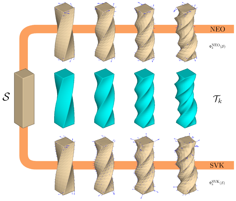
Figure 2: Deformation tracking experiment. The deformation sequence consists of 60 frames $\mathcal{T}_{k}$. In each frame the upper face of the beam $\mathcal{S}$ was twisted until a 360 degree twist was reached. The source $\mathcal{S}$ was then matched to each frame $\mathcal{T}_{k}$ while storing the result $\Phi_{k}(\mathcal{S})$ and gradually increasing the deformation. We show the result of the matching for four frames (90^∘, 180^∘, 270^∘ and 360^∘ twist) for the Neo-Hookean material model (upper row) and the Saint Venant-Kirchhoff Model (lower row). The optimized force vectors, measured on the coarse mesh $\mathcal{B}^{h}$, are shown on the results. The middle row shows the corresponding target frames (turquoise). The surface mesh $\mathcal{S}$ consisted of 14400 triangles while the tetrahedral mesh $\mathcal{B}^{h}$ on which the forces of the deformation are measured consisted of 1536 tets (567 surface triangles on $\partial\mathcal{B}^{h}$).

Our Matlab implementation was run on a standard desktop PC with 8GB of RAM and Intel Core i7 with 3GHz. The bottleneck routines such as the assembly of the tangent stiffness matrix were written in C. For SVK materials we wrote our own FEM code and for Neo-Hookean materials we modified the source code of CalculiX [21], a three-dimensional FEM software that is available under the GNU General Public License.

Computing the Initial Guess. Computing a reasonable initial guess is not straightforward and is mostly done in a heuristic manner. In the case that $\mathcal{S}$ and $\mathcal{T}$ only deviate by small deformations and rotations it is often reasonable to find initial correspondences simply by projecting points of the source mesh onto the target as done in a standard iterative closest point algorithm. In the case of large deformations and/or large rotations, however, nearest neighbor projection is usually a bad choice. The limitation of small deformations and rotations can partially be overcome by the use of shape descriptor like the heat kernel signature (HKS) [49] or wave kernel signature (WKS) [7]. These descriptors describe the diffusion of heat at each point or the dispersion in case of the WKS. Since these descriptors are based on the spectrum of the Laplace-Beltrami operator they are invariant under isometries, i.e., surface deformations that preserve geodesic distances. For large isometric or nearly isometric deformations one can then use a nearest neighbor search in the descriptor space for the first few iterations of Algorithm 1 instead of the Euclidean nearest neighbors. However, the so obtained correspondences can be treacherous, in particular in the presence of inner symmetries of the shape.

In our work we use a descriptor guided nearest neighbour search in the Euclidean space. As a shape descriptor we used the HKS. In the first few iterations we seek for each point on the source shape $\mathcal{S}$ k-nearest neighbours and then we select the one with the best matching HKS. We further assign a confidence value $w\in[0,1]$ for the correspondence and use only correspondences with confidence above a certain threshold. Similar weighting procedures have been used in [30, 16, 39]. The number $k$ of computed nearest neighbors was usually set around two to four percent of the number of nodes of the shape. After a few iterations we decreased $k$ down to one and passed on the confidence weighting what amounts to standard Euclidean nearest neighbours.

4.2 Experiments

Material Models. For our experiments we used the three material models introduced in Section 2. In the following we will refer to the small deformation model (17) as the linear model, to the Saint Venant-Kirchhoff model (15) as SVK and to the Neo-Hookean model (18) as NEO.

The first experiment is shown in Figure 2 and is supposed to demonstrate the flexibility of the two large deformation models (SVK and NEO). We took a triangular surface mesh $\mathcal{S}$ of a beam and created a sequence of deformations $\mathcal{T}_{k}$ (which we will call frames). In each frame we twisted the upper face of the beam while keeping the bottom face fixed until a twist of 360 degree was reached. We then used the frames $\mathcal{T}_{k}$ as target frames for matching $\mathcal{S}$ according to Algorithm 1. We start from frame $k=1$ and gradually increase the deformation while storing the resulting deformations $\Phi_{k}(\mathcal{S})$ until we reach the last frame. This is a very large deformation that causes high mechanical stress. Note that all mechanical quantities are measured with respect to the undeformed configuration $\mathcal{S}$.

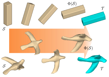
Figure 3: Our algorithm can find rigid motions. The target meshes $\mathcal{T}$ (transparent green, right) are rotations of the source meshes $\mathcal{S}$ (left). The bird mesh was taken from the SHREC data set. Our tet mesh had approximately 1400 tets compared to 18000 triangles of the surface mesh.

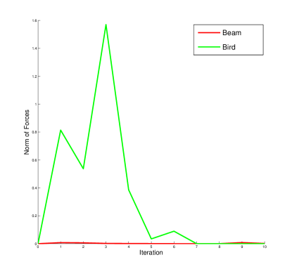
Figure 4: Discrete $L^{1}$-norm of the boundary forces in each iteration. The search space for the deformations is not confined to rigid motions but the deformation is “not far” from a rigid motion.

Here, we did not perform the smoothing described in step 3 in Algorithm1. In the first few steps both materials performed well. After a twist of approximately 270 degree we observed that the SVK model needed more iterations in each step to converge than the Neo-Hookean model. Also, the Newton-Raphson solver that is applied after every single optimization step needed more iterations to converge to an actual solution of the elasticity equations. The Neo-Hookean model, in contrast, showed a substantial computational robustness against this large deformation. The linear material model, i.e., the SVK model with linearized strain (no update of the tangent stiffness matrix in step 11 of Algorithm 1) failed to produce reasonable results much earlier. However, we do not show the linear case here since this material model is not suitable for this large deformation anyway.

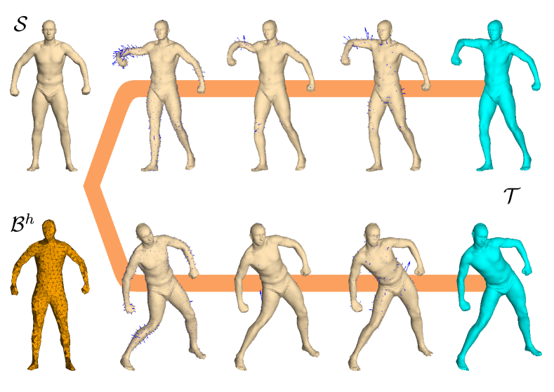
Figure 5: Several steps of the matching of a source shape (left, gray) to two different articulated human shapes (right, green) from the SCAPE dataset [5] are shown in the lower and upper row. The approximating volumetric mesh is shown on the left (orange) as well as the force vectors measured on the volumetric mesh. The force vectors are scaled for better visibility. The surfaces have approximately 25000 triangles. Our volumetric tessellation had approximately 2000 tets.

This coincides with our expectation since the SVK model is appropriate for large deformations but not suitable for large strain in contrast to the Neo-Hookean model which is suitable for both.

Invariances. As elaborated in Section 2 for each nonlinear material the deformation force measured by the second Piola-Kirchhoff stress (7) is invariant under rotations. However, in our numerical scheme we optimize a smoothed version of forces derived from the first Piola-Kirchhoff stress which is, in general, not invariant under rotations. Nevertheless, the magnitude of the forces is invariant but not the direction. For pure rotations the force is zero. Hence, we would like the matching algorithm to find pure rotations and to return a zero force. Figure 3 shows two examples. The initial guess of correspondences for the bird was made and updated using a nearest neighbour search in descriptor space in the first few iterations of our algorithm. For the rotated beam we simply used Euclidean projections since the HKS is “less descriptive” due to the high number of symmetries and hence might lead to an unreasonable initial guess.

The graphs in Figure 4 show the norm of the optimized boundary force in each iteration of the optimization. One can clearly see that in the first few iterations the optimized boundary force is not zero. This is to be expected since we do not restrict the search space of deformations to rotations. In the last few iterations the force is close to zero implying that our algorithm found a rigid motion of $\mathcal{B}^{h}$. The slightly incorrect matching of the rotated surface mesh of the bird, as seen in Figure 3 (bottom right), is due to the interpolation of the deformation of $\mathcal{B}^{h}$ to $\mathcal{S}$ and can be remedied by taking a finer tet mesh at the cost of computation time.

Last, we should mention that in case of a linear material model (Hooke’s law) the forces are not invariant under rotations but under infinitesimal rotations. These maps are the generators of the rotation group, i.e., they form the Lie algebra of $SO(3)$, and have skew symmetric derivatives. In two dimensions the effects of this invariance were demonstrated in [46]. Here, we will refrain from showing this.

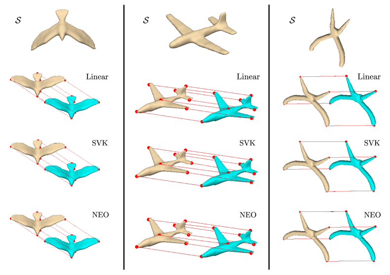
Figure 6: Examples from the SHREC dataset [26]. The source shapes are shown in the top row. We compare three material models: the linear model, the Saint Venant-Kirchhoff model (SVK) and the Neo-Hookean model (Neo). Several manually labeled landmark points of the source meshes are shown on the deformed source mesh and then compared to their corresponding landmarks in the target shapes (green). The SHREC surface meshes we used consist of 9000 to 14000 triangles and the tetrahedral meshes of 1600 to 2700 tets.

More Experiments. Figure 5 shows two examples of matching human poses. The models were taken from the SCAPE dataset [5]. Both poses were aligned using the SVK model. Note that the SCAPE dataset is nearly isometric and hence the HKS is nearly invariant under change of poses. This facilitates the nearest neighbor search in the first few iterations of our algorithm. Note that the external force found by our algorithm is sparse and mostly acts on the articulated parts of the model.

Examples of matching taken from the SCHREC dataset [26] are shown in Figure 6. Note that this dataset consists of usually non-isometric instances within each object class. Still, our algorithm produces good results.

	Linear	SVK	NEO
Birds
Norm of forces	6	14	2
# Iterations	14	35	36
Planes
Norm of forces	6.01	9.4	7.9
# Iterations	17	21	36
Pliers
Norm of forces	0.6	4.7	0.8
# Iterations	7	7	11

Table 1: Comparison of the three material models used on the examples of Figure 6. We show the sum of the norms of the force vectors and the number of iterations

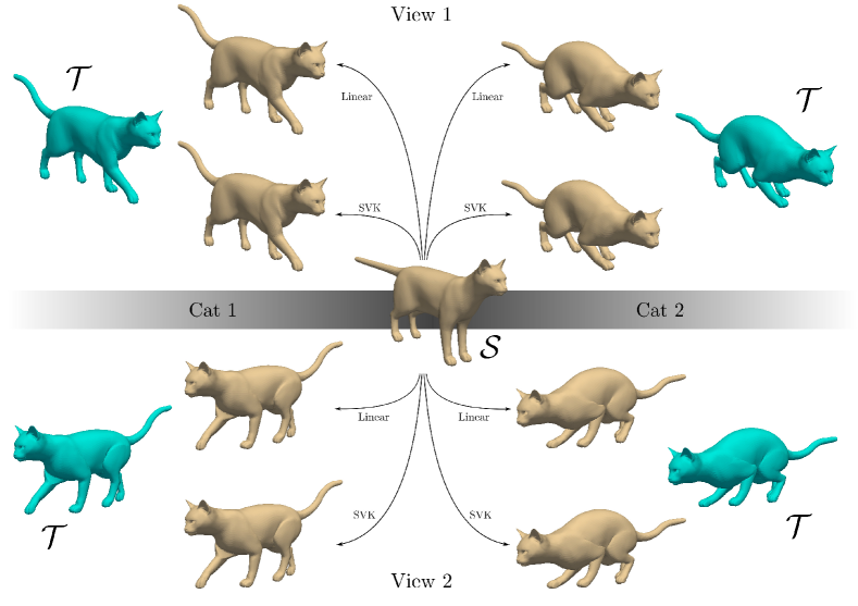
Figure 7: Two examples from the TOSCA dataset [13] from two different viewpoints (upper and lower row). The source (middle) is matched to the targets (green). Each shape in the TOSCA dataset consists of approximately 55000 triangles. The volumetric mesh we used consists of 1500 tets. Both results are of similar quality whereas the SVK model needed forces of higher magnitude.

Two examples taken from the TOSCA dataset [13] (left and right poses) are shown in Figure 7 from two different viewpoints (top and bottom). We used the SVK and the linear model, i.e., the SVK model without update of the tangent stiffness matrix (Hooke’s law), for each pose. Both results exhibit similar quality whereas the SVK model exhibits deformation forces that are higher in magnitude. This is in line with the comparison of the SVK model and the linear model in the experiment shown in Figure 6.

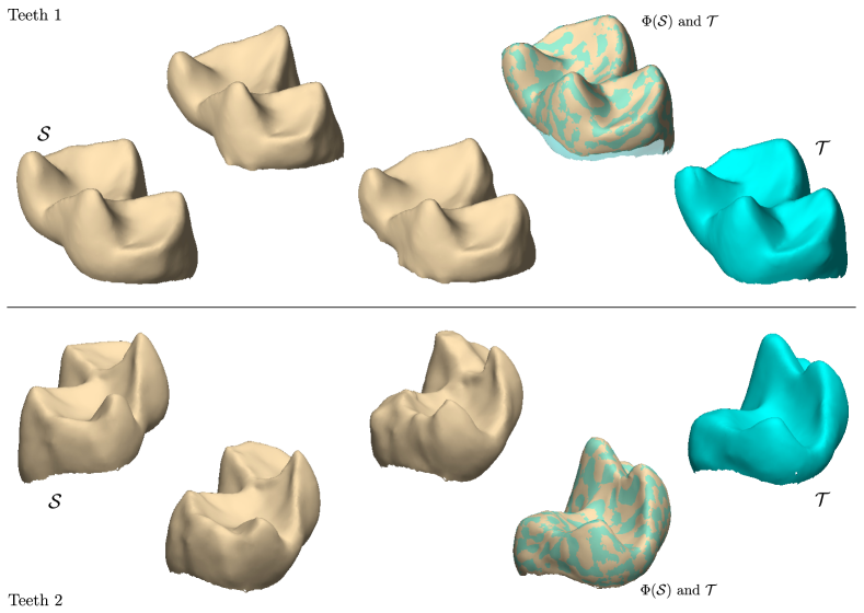
Figure 8: Two experiments performed on tooth shapes taken from the dataset of anatomical shapes of [9] (top and bottom row). The meshes have disk topology and the deformations are nonisometric and exhibit large strain. Several intermediate steps of the matching procedure of the sources (left, gray) into the target (right, green) are shown. We used the Neo-Hookean model. Each mesh we used has about 10000 triangles. The volumentric meshes that we created had about 1000 tets.

The experiments performed so far have been carried out on closed surfaces without boundary. However, the method is not restricted to closed surfaces provided one can create a volumetric mesh that represents the given object. To create the volumetric mesh it is usually necessary to fill holes. This, however, is the only step at which we use the closed surface. The rest of the steps follows the steps described in Algorithm 1. We demonstrate this in Figure 8. There we took two models of teeth from the anatomical dataset of [9] which exhibits quite large deformations. The deformation of the underlying tetrahedral mesh $\mathcal{B}^{h}$ is shown in Figure 9.

5 Discussion

In this work we propose a new ICP-like method in combination with a nonlinear regularizer for three-dimensional surface matching. The idea is to regard the surface as the surface of a physical body that can undergo elastic deformation. Our approach to finding a reasonable deformation is led by the assumption that the forces acting on the body are of a simple nature, i.e., we assume the forces are sparse, isotropic and act on the boundary only. This is, we believe, a reasonable assumption in many scenarios of shape deformation such as the change of a human pose.

We model the physical body as a hyperelastic material. The underlying equations, a nonlinearly coupled system of PDEs, is solved by means of a conformal FEM and needs to be supplemented with appropriate boundary conditions. We provide pure Dirichlet boundary conditions, i.e., the boundary deformation. This boundary deformation is in general unknown but one can give an initial guess. This initial guess induces a spring force between the source and the target that is supposed to drive the deformation of the source. We then use our proposed method to improve the initial guess such that the forces that act on the deformed body are sparse and isotropic according to the prior. This is done using the FEM which allows us to split the tangent stiffness matrix. The splitting we employ allows to connect boundary forces on the deformed body and boundary deformation of the source. This splitting generalizes the linear condensation methods that have been used in [11, 46] to the nonlinear case.

The optimization problem to be solved is nonlinear and computationally complex, depending on the shape and on the material model. We show how to approximate this problem by a sequence of convex problems that is solved in an iterative fashion with low computational demands. The convexification is done by successive linearization of the material model. The computational complexity is lowered by approximating the source surface with a coarser tetrahedral mesh. A deformation of the boundary of the volumetric tetrahedral mesh then naturally induces a deformation of the source surface by means of interpolation and smoothing. This amounts to a two-scale algorithm since the elastic properties are measured on the coarse scale while the provided initial guess

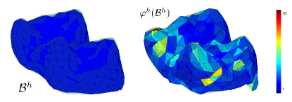
Figure 9: The volumetric mesh in rest state approximating the source shape shown in the top row of Figure 8 is shown on the left. The right side shows the deformed mesh after matching including the conformal distortion of each tet.

is a map on the (fine) source surface. Reducing the optimization problem to the boundary of the coarse scale volumetric mesh further reduces the dimensionality of the problem significantly.

Our method often delivers good results but can fail in certain cases. The estimated correspondences that need to be given before each iteration of the optimization is, at least in the first few iterations of our algorithm, usually computed by a Euclidean $k$-nearest neighbor search. Out of these $k$ nearest neighbors we pick the one with best matching HKS. In case of strongly non-isometric deformations or shapes with a high amount of intrinsic symmetry this will result in very unreasonable initial correspondences and the algorithm will get stuck in a local minimum. The case $k=1$ is the usual Euclidean nearest neighbor search and will give unreasonable correspondences in case of large deformations and/or rotations even if the deformation is isometric.

Another drawback is due to the coarse volumetric meshes. For example, a pure rotation of a coarse mesh does not necessarily induce a pure rotation of a fine mesh. The reason for this is that we essentially map a linearly interpolated map of the coarse mesh to the fine scale as described in Section 4.1 without incorporating information in normal direction. This effect is shown in Figure 10. Also, smoothing the deformation after interpolation can smear features such as corners of the deformed surface in an undesired way. Taking a finer volumetric mesh reduces this effect.

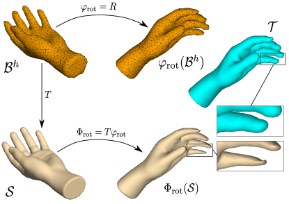
Figure 10: The effect of the interpolation of a pure rotation of the coarse mesh on the fine surface mesh. We chose a rotation $R\in SO(3)$ and constructed the map $T$ according to equation (47). The rotated coarse mesh (orange) is shown in the upper row. The bottom row shows the effect of the interpolated rotation on the fine mesh. We compare this to the rotated fine mesh (turquoise).

Furthermore, the method is not guaranteed to avoid element flipping due to the linearization and can exhibit high conformal element distortion, see Figure 9. Methods dealing with this problem in two and three dimensions can be found in [30, 36, 44] and can be integrated into our framework.

Finally, the computed boundary forces that are responsible for the shape change can be made invariant under rigid motion by a pull-back to the undeformed configuration. Hence, we believe, that they can serve as a comparison measure for different deformations of the same object since they measure how “difficult” it is to achieve the observed change.

Acknowledgments. This research was supported in part by the U.S.-Israel Binational Science Foundation, Grant No. 2010331, by the Israel Science Foundation, Grants No. 764/10 and 1265/14, by the Israel Ministry of Science, and by the Minerva Foundation. The vision group at the Weizmann Institute is supported in part by the Moross Laboratory for Vision Research and Robotics.

References

- [1] D. Aiger, N.J. Mitra, D. Cohen-Or 4-points Congruent Sets for Robust Surface Registration, ACM Transactions on Graphics Vol. 27, no.3 (2008)
- [2] M. Alexa, D. Cohen-Or, D. Levin As-rigid-as-possible Shape Interpolation, Proceedings of the 27th Annual Conference on Computer Graphics and Interactive Techniques (SIGGRAPH 2000)
- [3] B. Allen, B. Curless, Z. Popović The Space of Human Body Shapes: Reconstruction and Parameterization from Range Scans, ACM Transactions on Graphics Vol. 22, no. 3 (2003)
- [4] E.D. Andersen, K.D. Andersen The Mosek Interior Point Optimizer for Linear Programming: An Implementation of the Homogeneous Algorithm, Kluwer Academic Publishers, 197–232 (1999)
- [5] D. Anguelov, P. Srinivasan, D. Koller, S. Thrun, J. Rodgers, J. Davis SCAPE: Shape Completion and Animation of People, ACM Transactions on Graphics Vol. 24, no. 3, 408–416 (2005)
- [6] S.S. Antman Nonlinear Problems of Elasticity, Springer-Verlag, Applied Mathematical Sciences Vol. 107 (1995)
- [7] M. Aubry, U. Schlickewei, D. Cremers The Wave Kernel Signature: A Quantum Mechanical Approach To Shape Analysis, International Conference on Computer Vision (ICCV) - Workshop on Dynamic Shape Capture and Analysis (4DMOD), 1626–1633 (2011)
- [8] P.J. Besl, N.D. McKay A method for Registration of 3-D Shapes, IEEE Transactions on Pattern Analysis and Machine Intelligence Vol. 14, no. 2, 239–256 (1992)
- [9] D.M. Boyer, Y. Lipman, E.St. Clair, J. Puente, B.A. Patel, T. Funkhouser, J. Jernvall, I. Daubechies Algorithms to Automatically Quantify the Geometric Similarity of Anatomical Surfaces, Proc. Natl. Acad. Sci. (PNAS) Vol. 108, no. 45 (2011)
- [10] D. Braess Finite elements. Theory, fast solvers, and applications in solid mechanics, Cambridge University Press (2001)
- [11] M. Bro-Nielsen Finite Elements Modeling in Surgery Simulation, Proceedings of the IEEE Vol. 86, no. 3 (1998)
- [12] A.M. Bronstein, M.M. Bronstein, R. Kimmel Generalized Multidimensional Scaling: A Framework for Isometry-invariant Partial Surface Matching, Proceedings of the National Academy of Sciences of the United States of America (PNAS) Vol. 103, no. 5, 1168–1172 (2006)
- [13] A.M. Bronstein, M.M. Bronstein, R. Kimmel Numerical geometry of non-rigid shapes, Springer, 2008.
- [14] B.J. Brown, S. Rusinkiewicz Global Non-rigid Alignment of 3D Scans, ACM Transactions on Graphics Vol. 26, no. 3 (2007)
- [15] Y. Chen, G. Medioni Object Modeling by Registration of Multiple Range Images, Image and Vision Computing Vol. 10, no. 3, pp. 145–155 (1992)
- [16] J. Choi, A. Szymczak Fitting Solid Meshes to Animated Surfaces Using Linear Elasticity, ACM Transactions on Graphics Vol. 28, no.1 (2009)
- [17] H. Chui, A. Rangarajan A New Point Matching Algorithm for Non-rigid Registration, Computer Vision and Image Understanding Vol. 89, no. 2, pp. 114–141 (2003)
- [18] P.G. Ciarlet Mathematical Elasticity. Volume I: Three-Dimensional Theory, Series “Studies in Mathematics and its Applications”, North-Holland, Amsterdam (1988)
- [19] CGAL: Computational Geometry Algorithms Library, http://www.cgal.org
- [20] G. Dhondt The Finite Element Method for Three-Dimensional Thermomechanical Applications, Wiley (2004)
- [21] G. Dhondt, K. Wittig CalculiX: A Free Software Three-Dimensional Structural Finite Element Program, http://www.calculix.de
- [22] Q. Fang, D. Boas Tetrahedral Mesh Generation from Volumetric Binary and Gray-scale Images, Proceedings of IEEE International Symposium on Biomedical Imaging, 1142-1145 (2009)
- [23] M. Ferrant, S.K. Warfield, C.R.G. Guttmann, R.V. Mulkern, F.A. Jolesz, R. Kikinis 3D Image Matching Using a Finite Element Based Elastic Deformation Model, Proceedings of MICCAI 1999, LNCS 1679, pp. 202–209 (1999)
- [24] M.A. Fischler, R.C. Bolles Random Sample Consensus: A Paradigm for Model Fitting with Applications to Image Analysis and Automated Cartography, Comm. of the ACM Vol. 24, no. 6, 381–395 (1981)
- [25] N. Gelfand, N.J. Mitra, L.J. Guibas, H. Pottmann Robust Global Registration, Symposium on Geometry Processing,pp. 197–206 (2005)
- [26] D. Giorgi, S. Biasotti, L. Paraboschi SHape REtrieval Contest 2007: Watertight Models Track
- [27] M. Holden A Review of Geometric Transformations for Nonrigid Body Registration, IEEE Transactions on Medical Imaging Vol. 27, no. 1, pp. 111–128 (2008)
- [28] Q. Huang, B. Adams, M. Wicke, L.J. Guibas Non-Rigid Registration Under Isometric Deformations, Computer Graphics Forum Vol. 27, no. 5, pp. 1449–1457 (2008)
- [29] O. Van Kaick, H. Zhang, G. Hamarneh, D. Cohen-Or A Survey on Shape Correspondence, Computer Graphics Forum Vol. 30, no. 6, pp. 1681–1707 (2011)
- [30] S.Z. Kovalsky, N. Aigerman, R. Basri, Y. Lipman Controlling Singular Values with Semidefinite Programming, ACM Transactions on Graphics Vol. 33, no. 4 (2014)
- [31] P. Le Tallec Numerical Methods for Nonlinear Three-Dimensional Elasticity, Handbook of Numerical Analysis Vol. III, pp. 465–622 (1994)
- [32] Z. Levi, C Gotsman Smooth Rotation Enhanced As-Rigid-As-Possible Mesh Animation, IEEE Transactions on Visualization and Computer Graphics, 2015
- [33] H. Li, R.W. Sumner, M. Pauly Global Correspondence Optimization for Non-Rigid Registration of Depth Scans, Computer Graphics Forum. Vol. 27, no. 5 (2008)
- [34] Y. Lipman Möbius Voting for Surface Correspondence, ACM Transactions on Graphics (Proc. SIGGRAPH) Vol. 28, no. 3 (2009)
- [35] Y. Lipman, S. Yagev, R. Poranne, D.W. Jacobs, R. Basri Feature Matching with Bounded Distortion, ACM Transactions on Graphics Vol. 33, no. 3 (2014)
- [36] Y. Lipman Bounded Distortion Mapping Spaces for Triangular Meshes, ACM Transactions on Graphics Vol. 31, no. 4 (2012)
- [37] J. Löfberg YALMIP: A Toolbox for Modeling and Optimization in MATLAB, Proceedings of the CACSD Conference (2004), http://users.isy.liu.se/johanl/yalmip
- [38] A. Nealen, M. Müller, R. Keiser, E. Boxerman, M. Carlson Physically Based Deformable Models in Computer Graphics, Computer Graphics Forum Vol. 25, no. 4, pp. 809–836 (2006)
- [39] S. Rusinkiewicz, M. Levoy Efficient Variants of the ICP Algorithm, Proc. of the 3rd International Conference on 3-D Digital Imaging and Modeling (2001)
- [40] A. Quarteroni, R. Sacco, F. Saleri Numerical Mathematics, Second Edition, Texts in Applied Mathematics no. 37, Springer Verlag (2007)
- [41] R.D. Rabbit, J.A. Weiss, G.E. Christensen, M.I. Miller and the Applied Mechanics Group (Lawrence Livermore National Laboratories, Livermore CA) Mapping of Hyperelastic Deformable Templates Using the Finite Element Method, Proc SPIE 2573, pp. 252–265 (1995)
- [42] H. Si TetGen: A Quality Tetrahedral Mesh Generator and a 3D Delaunay Triangulator, http://www.tetgen.org
- [43] A. Savran, B. Sankur Non-rigid Registration of 3D Surfaces by Deformable 2D Triangular Meshes, Computer Vision and Pattern Recognition Workshops (CVPRW 2008)
- [44] C. Schüller, L. Kavan, D. Panozzo, O. Sorkine-Hornung Locally Injective Mappings, Computer Graphics Forum Vol. 32, no. 5, pp. 125–135 (2013)
- [45] T.W. Sederberg, E. Greenwood A Physically Based Approach to 2-D Shape Blending, ACM SIGGRAPH Computer Graphics Vol. 26, no. 2 (1992)
- [46] K. Simon, S. Sheorey, D. Jacobs, R. Basri A Linear Elastic Force Optimization Model for Shape Matching, Journal of Mathematical Imaging and Vision (2014)
- [47] O. Sorkine, M. Alexa As-rigid-as-possible Surface Modeling, Symposium on Geometry Processing Vol. 4 (2007)
- [48] R.W. Sumner, J. Schmid, M. Pauly Embedded Deformation for Shape Manipulation, ACM Transactions on Graphics Vol. 26, no. 3 (2007)
- [49] J. Sun, M. Ovsjanikov, L. Guibas A Concise and Provably Informative Multi-scale Signature Based on Heat Diffusion, Proceedings of the Eurographics Symposium on Geometry Processing, 1383–1392 (2009)
- [50] D. Terzopoulos, J. Platt, A. Barr, K. Fleischer Elastically Deformable Models, ACM Siggraph Computer Graphics Vol. 21, no. 4, pp. 205–214 (1987).