Extended H₂  emission line sources from UWISH2

Abstract

We present the extended source catalogue for the UKIRT Widefield Infrared Survey for H₂  (UWISH2). The survey is unbiased along the inner Galactic Plane from $l\approx 357\degr$ to $l\approx 65\degr$ and $|b|\leq$ 1^∘​​.5 and covers 209 square degrees. A further 42.0 and 35.5 square degrees of high dust column density regions have been targeted in Cygnus and Auriga. We have identified 33200 individual extended H₂  features. They have been classified to be associated with about 700 groups of jets and outflows, 284 individual (candidate) Planetary Nebulae, 30 Supernova Remnants and about 1300 Photo-Dissociation Regions. We find a clear decline of star formation activity (traced by H₂  emission from jets and photo-dissociation regions) with increasing distance from the Galactic Centre. About 60 % of the detected candidate Planetary Nebulae have no known counterpart and 25 % of all Supernova Remnants have detectable H₂  emission associated with them.

1 Introduction

The $\nu=$ 1 – 0 (S1) ro-vibrational line of molecular hydrogen at 2.122 $\mu$m is particularly bright in warm, dense, molecular environments (T $\sim$ 2000 K, $n_{\rm H}$ $\geq$ $10^{3}$ cm^-3). For this reason, this near-infrared line has been a much-used tracer of shocked molecular gas for a range of astrophysical phenomena, not least in outflows from the youngest protostars (e.g. Davis & Eisloeffel (1995); Stanke et al. (2002); Davis et al. (2009); Varricatt et al. (2010); Ioannidis & Froebrich (2012a); Bally et al. (2014); Hartigan et al. (2015); Zhang et al. (2015); Wolf-Chase et al. (2015, in prep.). H₂  may also be excited in photo-dissociation regions (PDRs) associated with young, intermediate-mass stars and Hii   regions (through fluorescence), as well as in post-AGB winds associated with Planetary and Proto-Planetary Nebulae (PNe; in shocks or again via fluorescence) or in Supernova Remnants (SNRs).

In late 2006 we defined UWISH2, the UKIRT Wide Field Imaging Survey for H₂ , as an unbiased, near-infrared, narrow-band imaging survey of the first Galactic quadrant. The region we initially targeted, covering an area between 10° $\leq$ $l$ $\leq$ 65° and $-$1^∘​​.5 $\leq$ $b$ $\leq$ $+$1^∘​​.5, includes most of the giant molecular clouds and massive star forming regions in the northern hemisphere. Our goal with UWISH2 was to complement existing and proposed near-, mid- and far-infrared photometric surveys such as the Spitzer Space Telescope GLIMPSE survey (Benjamin et al. (2003); Churchwell et al. (2009)), the Galactic Plane Survey (GPS, Lucas et al. (2008)) of the UKIRT Infrared Deep Sky Survey (UKIDSS, Lawrence et al. (2007)), the James Clerk Maxwell Telescope Galactic Plane Survey (Moore et al. 2015, subm.), the Herschel Space Telescope Hi-Gal survey (Molinari et al. (2010)), by utilising the H₂  1 – 0 S(1) line as a tracer of the dynamically active component of star formation (SF) not emphasised by the broad-band surveys.

Much of the UWISH2 survey area has also recently been imaged with the same telescope and instrument in narrow-band [FeII] line emission at 1.64 $\mu$m (the UKIRT Wide Field Infrared Survey for Fe⁺ – UWIFE; Lee et al. (2014)). These observations are certainly complementary to the H₂  imaging presented here since [FeII] is an excellent tracer of the higher-excitation atomic gas in shocks and collimated jets (e.g. Nisini et al. (2002); Giannini et al. (2002); Giannini et al. (2004)).

The UWISH2 survey was completed in 2011 and is described in (Froebrich et al., 2011). An extension to the survey, referred to as UWISH2-E, was proposed in late 2012. Between December 2012 and December 2013, our large mosaic of H₂  images of the Galactic Plane (GP) was extended down through the Galactic Center to $l$ $\sim$ 357° (although this extension does not cover the full width of the original survey at all longitudes - see Sect. 2.2). We also partially mapped two new fields, one available in the summer, the other in winter, around the well-known high mass star forming regions in Cygnus and the more quiescent molecular cloud complex in Auriga.

In this paper we present the results of an unbiased search for all extended H₂  emission line features in the UWISH2 and UWISH2-E surveys. We aim to provide a comprehensive catalogue of extended 1 – 0 S(1) features, their properties (position, size and flux) and most likely classification (as jet/outflow, PN, SNR or unclassified). This catalogue will be useful as a starting point for more detailed investigations of selected sub-sets of H₂  emission line objects, such as individual jets and outflows or PNe.

In Sect. 2 we describe the observations, survey areas, and data quality. In Sect. 3 we present the extended source catalogue and give a detailed account of the techniques used to find emission line features in the survey images. In Sect. 4 we discuss the overall properties of the detected H₂  emission line features, but refer to future publications for the detailed study of selected individual objects.

2 The UWISH2 and UWISH2-E Surveys

2.1 Observations

All data were acquired using the Wide Field Camera (WFCAM) on the United Kingdom Infrared Telescope (UKIRT), Mauna Kea, Hawaii. WFCAM houses four Rockwell Hawaii-II (HgCdTe 2048 $\times$ 2048 pixel) arrays spaced by 94 % in the focal plane. The pixel scale measures 0$\arcsec$​​.4, although micro-stepping is used to generate reduced mosaics with a 0$\arcsec$​​.2 pixel scale and thereby fully sample the expected seeing.

For both the UWISH2 and UWISH2-E surveys we essentially repeated the observing strategy adopted by the UKIDSS GPS (Lucas et al., 2008), the only difference being the choice of filter and the exposure time used. Individual 60 s exposures through a narrowband H₂  filter ($\lambda=2.122$ $\mu$m, $\delta\lambda=0.021$ $\mu$m) were repeated with a 2 $\times$ 2 point micro-stepping at three jitter positions. In this way 12 exposures were acquired at each telescope pointing, resulting in a total exposure time per pixel of 720 s. Four telescope pointings are needed to fill in the gaps between the detectors; 16 mosaic images thus constitute a tile covering about 0.75 square degrees.

All data were reduced by the Cambridge Astronomical Survey Unit (CASU), which is responsible for data processing prior to archiving and distribution by the Wide Field Astronomy Unit (WFAU). The CASU reduction steps are described in detail by Dye et al. (2006); astrometric and photometric calibrations were achieved using 2MASS (Dye et al. (2006); Hewett et al. (2006)). The reduced images are available from WFAU as well as from the UWISH2 website, along with the corresponding broad-band J, H and K images from the GPS data. Continuum-subtracted H₂ $-$K images are also available, as are colour renditions of each 16-image tile.

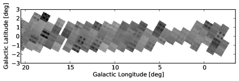
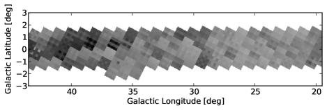
Figure 1: Plots of the seeing distribution in the Galactic Plane area of the survey. Positions covered by tiles/images with worse seeing are indicated by darker colours. See Sect. 2.3 for more details.

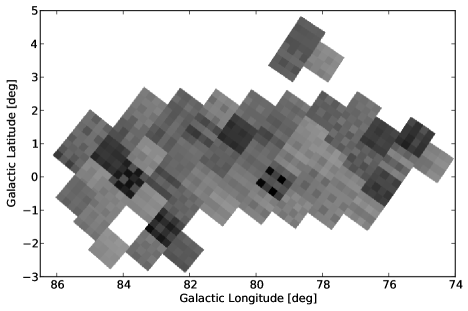
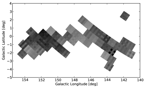
Figure 2: As Fig. 1 but for the Cygnus (top) and Auriga (bottom) area of the survey.

2.2 Target Area

The survey covers the northern GP as well as selected high dust column density regions in Cygnus and Auriga. Along the GP we covered a longitude range from $l\approx 357\degr$ to about $l\approx 65\degr$. For most of this longitude range the survey covers the region $|b|$ $\leq$ 1^∘​​.5. There are some extensions towards the North at $l$ $\approx$ $19\degr$ and towards the South at $l$ $\approx$ $36\degr$. Furthermore, due to time constraints we were unable to complete the full latitude range near the Galactic Centre. Figures 1 and 2 show the detailed coverage along the GP and in Cygnus and Auriga. In total we have observed 268 tiles with coverage in H₂  and the UKIDSS GPS K-band. Note that we have observed one additional tile just South of the Galactic Centre, but there is no K-band counterpart in the GPS database. We have searched the image for H₂  emission, but no features were detected.

Considering the overlap between images and tiles, the total area covered along the GP is 209 square degrees. In the Cygnus and Auriga areas the fields are roughly concentrated along the GP, but preference has been given to high extinction regions. Full coverage of the entire cloud complex could not be obtained due to time constraints. We have observed 54 tiles in Cygnus and 45 tiles in Auriga. Considering the overlap of images, this corresponds to 42.0 and 35.5 square degrees, respectively. Hence the total area covered in the entire UWISH2 survey is 286.5 square degrees.

Due to the nature of the observations, the coverage in both Galactic longitude and latitude in the survey area is not homogeneous. Hence any investigations of distributions of objects along and perpendicular to the GP will have to be corrected for the variations in relative coverage, i.e. a factor proportional to the number of images obtained at a specific latitude/longitude. In the top left panel of Fig. 3 we show the relative coverage (normalised to a maximum of one) perpendicular to the GP. As can be seen, within 1^∘​​.3 of the GP, the relative coverage exceeds 90 % and is more or less homogeneous. Further away from the GP the coverage steeply declines and sinks below 10 % at about 1^∘​​.8 from the GP. A 50 % coverage is achieved for all areas with $|b|<$ 1^∘​​.5. In the bottom left panel of Fig. 3 we show a similar graph for the coverage along the GP. Between $l=7\degr$ and $l=65\degr$ the coverage is almost constant. Larger discrepancies are only seen near the GC and the two areas where we observed additional tiles slightly further away from the GP (at $l\approx 18\degr$ and $l\approx 35\degr$). For completeness, we also show the coverage distributions for the Cygnus and Auriga regions in the middle and right columns of Fig. 3, respectively. Due to the more patchy distribution of tiles in these clouds, the relative coverage in these cases is much more variable than along the GP.

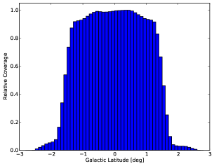
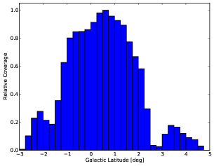
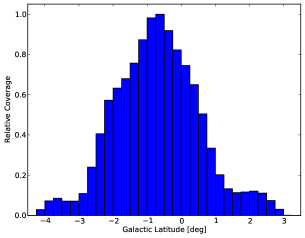
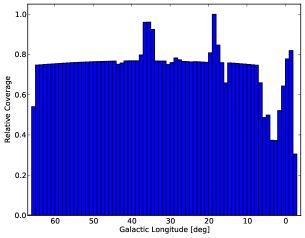
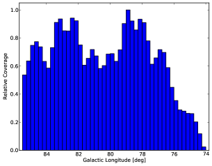
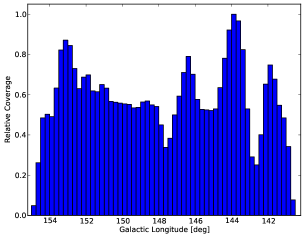
Figure 3: Relative latitude (top row) and longitude (bottom row) coverage of the survey in the Galactic Plane (left column), Cygnus (middle column) and Auriga (right column) area of the survey. The relative coverage is proportional to the number of images taken at a specific latitude/longitude and is normalised to a maximum of one. These distributions are used to correct observed distributions of objects such as Jets and PNe to account for the variations in coverage along and across the GP.

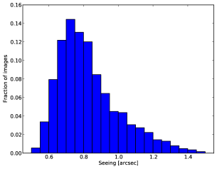
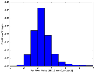
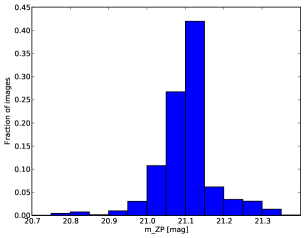
Figure 4: Data quality of the survey. The left panel shows the seeing distribution of our images , the middle panel the one sigma per pixel noise distribution and the right panel the distribution of the photometric zero point mag$\_$zp. The median seeing is 0$\arcsec$​​.8 and about 83 % of the data has been taken with a seeing of less than one arcsecond. The median one sigma per pixel noise is 3.25 $\times$ $10^{-19}$ W m^-2 arcsec^-2.

2.3 Data Characteristics

The distribution of seeing values in our survey can be found in the left panel of Fig. 4. How these values are distributed spatially can be seen in Figs. 1 and 2. The median seeing in the survey is 0$\arcsec$​​.79, with 82.9 % of the area observed at seeing values of below one arcsecond. Most of the poorer seeing data is distributed in the additional regions in Cygnus and Auriga. There, however, the crowding of stars is much less severe than in the inner GP, hence slightly worse seeing will not affect the detection and photometry of extended H₂  features.

We determine the background per pixel noise level in the images by estimating the rms scatter of the pixel values from the background, using a 3 sigma clipping procedure to remove stars. The counts are then converted into a surface brightness using the mag$\_$zp values and integration times (for details see the calibration of photometry in Sect. 3.2). The distribution of the one pixel 1$\sigma$ noise for all images is shown in the middle panel of Fig. 4. The median one pixel noise is $3.25\times 10^{-19}$ W m^-2 arcsec^-2, in agreement with the typical noise in the original UWISH2 area (Froebrich et al., 2011). Averaged over the median seeing from above, which covers about 16 pixels, the typical 5$\sigma$ noise or surface brightness detection limit is $4.1\times 10^{-19}$ W m^-2 arcsec^-2. Alternatively, the 3$\sigma$ noise over 1$\arcsec$​​.2, the Glimpse pixel size, is $1.6\times 10^{-19}$ W m^-2 arcsec^-2.

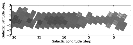
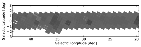
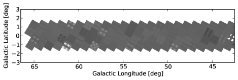
Figure 9: Plots and mag$\_$zp distribution in the Galactic Plane area of the survey. Darker colours indicate higher values for mag$\_$zp.

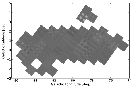
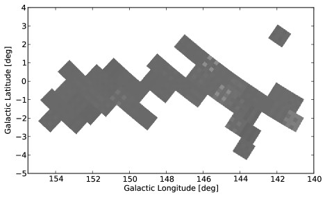
Figure 10: As Fig. 9 but for the Cygnus (top) and Auriga (bottom) area of the survey.

In the right panel of Fig. 4 we show the distribution of the photometric zero point values in the images. The narrow peak around 21.1 mag indicates that about two thirds of all images were taken under comparable atmospheric conditions, with extinction variations of less than 5 %. This can also be seen in the Figs. 9 and 10 in the Appendix. We also summarise all the data for every image in the Appendix in Table LABEL:imagedatatable. There we list the tile containing the image, the image name (containing the observation date), the centre of each image in RA, DEC (J2000) and l,b, the seeing, the calibration magnitude zero point and its uncertainty as well as the estimated one pixel surface brightness noise.

3 The Extended Source Catalogue

In this section we describe the extended H₂  emission line object catalogue obtained from the UWISH2 images.

3.1 Source detection

To obtain an, as much as possible, complete and unbiased catalogue of extended H₂  emission line features, we performed the following steps for all images: i) Continuum subtraction of the emission line images; ii) Filtering and automated detection of extended H₂  features; iii) Manual verification and removal of image artifacts. These steps are performed as described in detail below.

3.1.1 Continuum Subtraction

To remove the continuum emission from the H₂  narrow band images we utilised the K-band data from the UKIDSS GPS (Lucas et al., 2008). This continuum subtraction was done on an image by image basis, i.e. run separately for each 4k$\times$4k image. Most of our H₂  images were taken at exactly the same positions as the GPS K-band data, with off-sets of less than a fraction of an arcminute. For a small fraction of fields, the off-sets were larger than one arcminute. In these cases we combined the K-band images from the GPS to obtain a matching K-band image utilising the Montage software. The image subtraction routine aligns the H₂  and K-band images, determines the scaling factor for the continuum image and uses psf-fitting to subtract the stars. The K-band scale factor and the psf shape are determined from unsaturated, isolated stars in 1000 pix $\times$ 1000 pix sub-images. The details of the procedure are described in Lee et al. (2014). Note that the fluxes in the H₂  images are unchanged, and only the K-band continuum data are scaled.

These H₂ $-$K difference images show many real H₂   emission line objects (such as shock excited Jets, SNRs or PNe), but also a large number of H₂  false positives caused by image and data analysis artifacts, as well as variability. In Fig. 5 we show six examples of such potential false positives. Stars which are saturated or near the saturation limit (of about K=11 mag) are not subtracted completely. Furthermore, the K-band and H₂  images are typically taken several years apart from each other. Hence, any object that is variable, such as some giant stars or YSOs, might leave a positive or negative residual in the difference images, as do high proper motion stars. Furthermore, several kinds of image artifacts, such as reflections, memory effects from bright stars, and electronic cross-talk also leave residuals resembling H₂  emission line features. Finally, in cases where the two images had very different seeing, most stars were not removed completely.

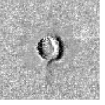
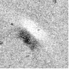
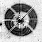
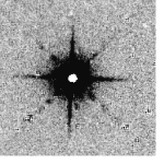
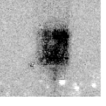
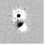
Figure 5: Example of false positives in the H₂ $-$K difference images. Suspected H₂  bright features are darker. From the top left to the bottom right, the panels show the following: i) electronic cross-talk from bright stars; ii) reflections from very bright stars; iii) diffraction rings around bright stars; iv) a variable (brighter during H₂  imaging) and saturated star; v) reflection from bright star just outside the edge (at bottom) of an image; vi) high proper motion star (next to variable star – fainter during H₂  imaging.

3.1.2 Extended Source Detection

Most of the real H₂  features in our images are spatially resolved and have a low surface brightness. Furthermore, many of the extended features are projected onto a spatially variable background. Hence, before the detection of these extended, low surface brightness features, we filtered our images to remove remaining point sources and large scale variable background. We replace any small-scale structures (less than 2″ x 2″) that have a pixel value exceeding the 5$\sigma$ noise in the images with the local background. This will remove most un-subtracted point sources. We determined the local background as the median pixel value within 20″ and subtracted it from the H₂ $-$K difference images. Note that this will remove some of the largest scale features such as extended Hii  regions from the catalogue. However, in most cases a significant fraction of this emission will still be detected as several individual, smaller features. Hence in general we will have some detections of most extended objects. Readers interested in particular, very extended objects should however, re-process our H₂ $-$K difference images with an appropriate spatial filter.

We identified every region in the background subtracted and point source removed images which was larger than four square arcseconds and had pixel values above half the rms noise in the images. This was done by plotting contours in ds9 at the respective level. The shape of each closed contour is described by a polygon and is referred to as a ’region’ hereafter. The minimum size limit is essential to remove most of the remaining point sources and noise from the list of objects. We rejected every region that had a 2MASS point source within three arcseconds from the region centre to also automatically remove the majority of saturated stars from our list. Furthermore, many very bright stars (K $<$ 7 mag) showed diffraction rings (e.g. top right panel in Fig. 5) that our procedure would pick up. We thus also removed every region that was completely within 35″ (slightly larger than the radius of the diffraction rings) from one of these very bright stars. Finally, all regions within 10″ from the edge of an image are removed. Note that the overlap between images is generally larger than this, hence no objects are lost in gaps. There is a small number of objects which have indeed multiple entries in the catalogue as they are detected (in whole or in part) on more than one image. We have not removed or joined these multiple entries in the final catalogue.

The requirements for the automated source detection (4 square arcseconds above the 0.5 $\sigma$ single pixel noise level), combined with the 0$\arcsec$​​.2 $\times$ 0$\arcsec$​​.2 pixel size, can be used to estimate the detection limit. In essence the software will pick out any extended object whose surface brightness is higher than the 5 $\sigma$ one pixel noise listed for every image. The one pixel noise values for all images are listed Table LABEL:imagedatatable in the Appendix.

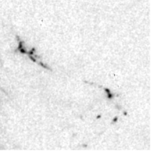
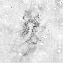
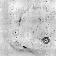
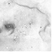
Figure 6: Example of real objects in the H₂ $-$K difference images for each of our object categories. Suspected H₂ –bright features are darker. From the top left to the bottom right, the panels show the following: i) ’j’ – outflow from IRAS 20294+4255; ii) ’p’ – Planetary Nebula SH 2-71; iii) ’s’ – Supernova remnant G11.2$-$0.3; iv) ’u’ – Emission near the cluster VDB 130.

3.1.3 Source verification/classification

The above automated detection procedure still included a large number of regions which were obviously not real H₂  features, and removed others which happened to be in the vicinity of bright stars. Hence, we manually checked all images to remove any region that was obviously not a real H₂  feature, e.g. image artifacts, variable or saturated stars and to re-add regions that were removed but clearly real. About 35 % of all images were searched by two people independently to gain an understanding of the completeness and contamination of the selected H₂  features. The remaining images were only searched by one person. Based on the comparison of the catalogues obtained for the images with two people selecting objects as real, we estimate that the contamination of the catalogue with image artifacts or noise is very small. At most 1 – 2 % of the catalogue entries might be artifacts. Also the completeness of the catalogues is very high. We estimate that more than 95 % of all the real H₂  features detected automatically are in the final catalogue. Missing objects are usually small features in regions of large extended H₂  emission. These missing objects do not contribute with any significance to the total area or flux of the H₂  emission line catalogue.

During the above discussed manual verification of the automatically selected H₂  features, we also classified each feature into one of four categories: i) ’j’ for all objects which seem to be part of a Jet or outflow from a young star. This classification was based on the shape of the feature, as well as its appearance/colour in the JKH₂  colour images. E.g. isolated, extended, high surface brightness H₂  knots which are situated in or near obvious star forming regions are classified as jet/outflow; ii) ’p’ for objects that resemble known PNe. These tend to be ring-like, bipolar or in some cases more complex structures, typically not related to star forming regions. Note that in some cases the appearance alone is not sufficient to distinguish a bipolar PN from a Jet emanating from a young star. We furthermore checked the positions of all known PNe and candidates in the survey area and classified all H₂  features as ’p’ if they were within a few arcsecond of a known object. We utilised the PNe entries in SIMBAD and the catalogues from IPHAS (Sabin et al., 2014), MASH (Parker et al., 2006) and MASH2 (Miszalski et al., 2008); iii) ’s’ for objects which are most likely part of a Galactic SNR. All H₂  features within the area of a known SNR (we utilised the list of Green (2009)) were selected to be of this category if they were not part of an obvious PN or Jet/outflow, or a small individual feature with no resemblance of the H₂  emission in other SNRs; iv) ’u’ for all objects which could not be assigned to any of the other three categories. Note that the vast majority of these features are most likely part of PDRs surrounding Hii  regions. Thus, we refer to all the unclassified regions as PDRs. In Fig. 6 we show one example of each of the object categories.

Note that the source selection and classifications (except for the SNRs and the known PNe) were done blind, i.e. without using any catalogues of known objects or SIMBAD. This hence gives us a further estimate of the completeness and accuracy of the classification by comparing to lists of known objects. We utilised the catalogue of Molecular Hydrogen emission line Objects (MHOs) from Ioannidis & Froebrich (2012a) who manually searched about 33 square degrees of early UWISH2 data for emission from jets and outflows. They list 134 MHOs and we have checked what fraction of these are contained in our catalogue: 83 % of the MHOs are included in our extended–H₂  feature catalogue. Exclusively all of the non-detections (17 %) are faint and small H₂  features which in most cases are similar to variable point sources rather than H₂  emission line objects. Of the detected H₂  features, 79 % are also classified as being part of a jet or outflow, 15 % are not classified (’u’), 4 % coincide with emission from SNRs and 2 % (2 MHOs) are listed as PN candidates in our list. Hence any objects missing in our catalogue are most likely faint and compact – indistinguishable from variable point sources.

3.2 Photometry

Flux measurement and calibration

Photometry has been obtained for each region in the H₂ $-$K images. As these difference images are obtained by only scaling the K-band continuum fluxes, the H₂  flux in all the images is conserved. We identify all pixels inside each region and determine their median, maximum and total number of counts. We then correct these values by the local background counts. These are estimated as the median count value in a ring around each region with an inner radius equal to the radius of the region and an outer radius of twice this. Note that in some rare cases, this background estimate will be wrong, e.g. if a small region is situated close to a larger region of extended H₂  emission. These occurrences are rare, but might lead to background corrected fluxes which are erroneous or even negative. For a further discussion of uncertainties of the photometry see the end of this Section.

We convert the counts in each region into fluxes or surface brightness in two steps. Firstly the counts are converted into a magnitude via:

$$m=m_{\tt zp}-0.05\cdot\left(X-1\right)-2.5\cdot\log_{10}\left(\frac{\tt counts}{t_{exp}}\right)-m_{\tt ap}$$ (1)

where $m_{\tt zp}$ is the magnitude zero point for the observations, $X$ the airmass during the observations, $t_{exp}$ the exposure time in seconds and $m_{\tt ap}$ the aperture correction. As we are only considering extended sources we can set the aperture correction term to zero. All other terms are obtained from the FITS header in the H₂  images. Note that all our observations are taken with 720 s integration time per pixel and the airmass is always between one and two. Hence, in most cases, the airmass term is of the same order or smaller than the uncertainty in $m_{\tt zp}$. Furthermore, as can be seen in the right panel of Fig. 4, the general variations in $m_{\tt zp}$ are also only of the same order of magnitude. Note that $m_{\tt zp}$ includes the corrections that need to be made caused by the micro-stepping and hence 0$\arcsec$​​.2 pixel size in our data.

These magnitudes are converted into fluxes by:

$$F=F_{0}^{H_{2}}\cdot 10^{-\frac{m}{2.5}}$$ (2)

The $m_{\tt zp}$ values will calibrate the magnitudes into the 2MASS K-band. We thus used the 2MASS K-band flux zero point of 4.283$\cdot$10^-10 W m^-2 $\mu$m^-1 from Cohen et al. (2003) and the K-band filter width of 0.262 $\mu$m to determine the flux zero point $F_{0}^{H_{2}}=1.12\cdot 10^{-10}$ W m^-2. In combination the flux $F$ corresponding to counts is determined as:

$$F={\tt counts}\cdot\frac{1.12\cdot 10^{-10}Wm^{-2}}{t_{exp}[s]}\cdot 10^{\left\{-\frac{m_{\tt zp}-0.05\cdot\left(X-1\right)}{2.5}\right\}}$$ (3)

We compared our calibrated flux values to published flux values of jet knot and SNRs and they agree at the 10 % level. Conversion of fluxes into surface brightness is done using the pixel size of 0.04 square arcseconds in our images.

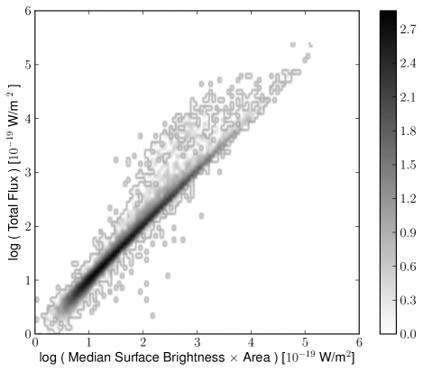
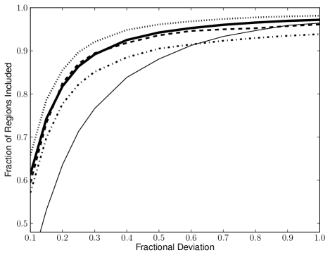
Figure 7: Top: Comparison of total flux and median surface brightness times area for all detected objects. The gray scale indicates the Log of the density of objects in each position. Most objects are very close to the 1:1 line. Bottom: Fractional deviation of the two flux estimates from the top panel vs. the fraction of objects which have a deviation smaller than it. The different line styles indicate the various objects: dot-dash line for SNRs, dashed line for PNe, bold solid line for all objects, dotted line for PDRs, thin solid line for jet features.

Total flux estimates for objects

There are two ways to determine the entire H₂  flux of a region. We can: i) use the background corrected total flux inside a region ($F_{tot}$), or we can ii) multiply the background corrected median surface brightness by the area (or median flux) of the region ($F_{med}$). Both ways have obvious drawbacks. If the region contains a non-subtracted residual, either due to a saturation or variability (see also Fig. 5), then the total flux can be influenced (positively or negatively) by the presence of the star. If the median surface brightness is not a good estimate of the average H₂  flux, e.g. when a small fraction of the region contains a large fraction of the flux, the total flux will be underestimated. In order to compare the two methods we compare the estimated fluxes for both in the top panel of Fig. 7. It shows the density of objects, and in the majority of cases the two H₂  flux estimates are comparable. There are, however, a number of cases where the two estimates disagree by a large amount.

We investigate for what fraction of objects the two flux estimates agree within a given range. This is shown in the bottom panel of Fig. 7. The x-axis in the plot is the fractional deviation of the two fluxes (from 10 % to a factor of two) and the y-axis shows the fraction of objects with a deviation smaller than this. The different line styles indicate the various object types. The bold solid line is for all objects, the thin solid line for jet features, the dotted line for PDRs, the dashed line for PNe and the dot-dash line for SNRs. As one can see from the figure, for about 80 % of all objects the deviation of the two flux estimates is less than 20 %. For the jet features the agreement is clearly worse, with only about 65 % having flux estimates with a better than 20 % agreement.

The reason for the latter seems to be the surface brightness distribution within jet knots. Most of them contain a small number of pixels which contribute a large fraction of the flux. This seems to be less an issue for PNe, PDRs and SNRs. We hence recommend to use $F_{tot}$ for the total fluxes of all objects classified as jet, while for the other object types $F_{med}$ seems more appropriate, as it prevents the potential inclusion of flux from (unsubstracted or variable) stars projected onto the H₂  emission line object. However, should the reader require more accurate photometry of selected objects, we recommend that they redo the flux estimate in our images, ensuring that only H₂  emitting areas are included in the photometry.

3.3 Object groups

Many of the detected H₂  emission features are not isolated, but are rather part of a group of objects. This is particularly true for the PNe and SNRs, which often consist of several emission features due to low surface brightness or large extent. We have hence grouped regions according to their spatial distribution. Objects were considered part of a group if they had a nearest neighbour within a given angular distance. For each group we determined properties such as the position, size (as the radius of a circle enclosing all group members) and total flux.

In the case of PNe regions, these groups can be considered as actual PN. We grouped objects automatically if they were separated by less than 3 arcminutes. Additionally we inspected all of these PNe visually to ensure that there were no two PNe closer to each other than the 3’ threshold and that the extended PNe in the catalogue had no ’outlying’ features that were classified as a separate PN.

For the Jets and outflows it is not a simple task to identify which jet knots are part of which outflow and which object is the actual driving source of the jet. Such a procedure needs a detailed study of each region and is beyond the scope of this paper. However, groups of Jet/outflow knots can be considered as star forming regions with actively accreting YSOs. Given that a typical distance of jets and outflows in the survey area is about 3.5 kpc (Ioannidis & Froebrich, 2012b) and the jets seem to occur in small groups of about 5 pc size (Ioannidis & Froebrich, 2012a), we used 0^∘​​.1 as minimum distance to separate groups of jets and outflows. Hence, these groups can be viewed as very young active star forming regions, slightly more extended than a typical young cluster (e.g. Schmeja et al. (2008)). Note that if moved to 3 kpc, the jets and outflows in NGC 1333 would be distributed over an area of about 2’ x 2’ on the sky.

The objects classified as ’u’ (most likely Hii  regions or PDRs) are also grouped with the same minimum distance of 0^∘​​.1, as they are probably at the same typical distances as the jet and outflow features. In essence these groups are likely to represent more evolved regions of star formation where the H₂  emission is caused by sources of ionising radiation.

We do not group the SNR objects in the same way as the other object types, since many of the SNRs are very extended on the sky. Instead, we have manually selected all the H₂  features which are part of each of the identified SNRs.

3.4 Catalogue description

The full extended H₂  feature catalogue displayed in Table LABEL:objectdatatable contains the following columns:

1. Object ID; this is derived from the Galactic coordinates of the centre of each region. As centre we use the geometric centre of the polygon enclosing the detected H₂  emission.

2. Right Ascension and Declination (J2000) of the centre of the emission region.

3. Area $A$ of the emission region in square arcseconds.

4. Radius $r$ of the emission region in arcseconds; This is the minimum radius of a circle around the centre of the region that is enclosing all the emission.

5. Median surface brightness F${}_{sb}^{med}$ of the region in 10^-19 W m^-2 arcsec^-2; This is the surface brightness determined from the background corrected median intensity in the region.

6. Peak surface brightness F${}_{sb}^{max}$ of the region in 10^-19 W m^-2 arcsec^-2; This is the peak surface brightness of the region. It might be influenced by the presence of stars inside the region.

7. One pixel rms noise surface brightness F_σ in 10^-19 W m^-2 arcsec^-2; This is the one sigma rms of the background in a ring with inner radius $r$ and outer radius $2r$ around each region (determined after sigma clipping to remove remaining stars and real emission features).

8. Total brightness F^totof the region in 10^-19 W m^-2; This is the total flux measured in each region. It might be influenced by the presence of stars inside the region. An alternative measure of the total flux would be the product of the median surface brightness and area of the region.

9. Relative uncertainty $\Delta F/F$, in percent, of all fluxes due to the uncertainty in the magnitude zero point of the observations $\Delta m_{\tt zp}$.

10. Classification $C$ of the object; This is a letter indicating what kind of object the region is most likely a part of. These are: j – jet or outflow from a YSO; p – part of a PN; s – part of a SNR; u – unknown nature, most likely part of a PDR near an Hii  region.

11. Name of the tile the region is on.

12. Name of the image the region is on.

13. Group identifier the object belongs to. The group identifier contains the object type, as well as the Galactic coordinates of the group, calculated as the geometric centre of the features that make up the group.

4 Results and Discussion

In this paper we will only discuss the general distribution and properties of the detected H₂  emission regions. For a detailed discussion of individual objects, or groups of objects we refer the reader to publications in preparation.

Table 1: Table showing the different parts of the survey used in the analysis and some of the accumulated properties of the objects identified in them. We list the survey area, the sum of the total fluxes for each of the four object types and the total number of identified groups of objects. Note that for PNe and SNRs a ’group’ identifies individual objects, while for Jets and PDRs a group simply refers to a group of spatially related individual H₂  features. The numbers in brackets indicate the fraction (as percent, rounded to the nearest integer) of the total flux or numbers of the total in the entire survey. We separate inner and outer GP at $l=$ 30° and list all values for both together in the additional row labeled ’GP’.

Region	Area		F${}_{\rm tot}^{\rm Jet}$	F${}_{\rm tot}^{\rm PDR}$	F${}_{\rm tot}^{\rm PN}$	F${}_{\rm tot}^{\rm SNR}$		NJet	NPDR	NPN	NSNR
	[deg2 (%)]		[10-14 W m-2] (%)					[Number (%)]
Total	286.45		10.6	49.6	7.67	46.1		711	1309	284	30
GP	209.00 (73)		4.70 (44)	30.3 (61)	7.37 (96)	46.1 (100)		450 (63)	925 (71)	261 (92)	30 (100)
GP (Inner)	95.18 (33)		2.83 (27)	24.7 (50)	5.73 (75)	15.5 (34)		253 (36)	489 (37)	112 (39)	20 (67)
GP (Outer)	113.79 (40)		1.86 (18)	5.58 (11)	1.64 (21)	30.6 (66)		197 (28)	436 (33)	149 (52)	10 (33)
Cygnus	41.99 (15)		5.73 (54)	18.3 (37)	0.24 (3)	—		210 (30)	353 (27)	16 (6)	—
Auriga	35.46 (12)		0.12 (1)	1.13 (2)	0.055 (1)	—		51 (7)	31 (2)	7 (2)	—

Table 2: Table listing the density (G, in objects per square degree) of the groups of objects in the various parts of the survey. We also list the median total flux ($\bar{\rm F}_{\rm tot}$ in 10^-19 W m^-2) for each kind of group of objects. Note that for PNe and SNRs a ’group’ identifies individual objects, while for Jets and PDRs a group simply refers to a group of spatially related individual H₂  features. We separate inner and outer GP at $l=$ 30° and list all values for both together in the additional row labeled ’GP’.

Region	GJet	GPDR	GPN	GSNR	$\bar{\rm F}_{\rm tot}^{\rm Jet}$	$\bar{\rm F}_{\rm tot}^{\rm PDR}$	$\bar{\rm F}_{\rm tot}^{\rm PN}$	$\bar{\rm F}_{\rm tot}^{\rm SNR}$
	[objects deg-2]				[10-19 W m-2]
Total	2.48	4.57	0.99	0.10	193	149	441	7096
GP	2.15	4.43	1.25	0.14	207	137	453	7096
GP (inner)	2.66	5.14	1.18	0.21	298	228	570	4345
GP (outer)	1.73	3.83	1.31	0.09	160	86.1	366	18120
Cygnus	5.00	8.41	0.38	—	204	183	173	—
Auriga	1.44	0.87	0.20	—	74.5	203	376	—

4.1 General Distributions

The entire survey region is composed of 5872 individual images. In only about one third of them (1935) have we identified real H₂  emission line features. This indicates that most areas, especially along the GP, are devoid of detectable H₂  emission, and that the detected H₂  features are localised/clustered. In total we detected 33200 individual extended H₂  emission line features. About 62 % of them are situated in fields along the GP (37 % in the inner and 25 % in the outer GP – separated at $l=$ 30°), about 36 % are in the Cygnus area, and the remaining 2 % are in Auriga. Detailed results for the identified groups of objects are outlined in Tables 1 and 2. In these tables we break down the numbers for each of the survey regions for the different object classes (Jets, PNe, SNRs, unclassified – most likely PDRs). Furthermore, we show the total area covered by each part of the survey. We list the number of PNe, SNRs, the number of Jet groups (actively accreting star forming regions) and groups of other H₂  emission features, as well as their total fluxes, median fluxes and projected object densities in the different parts of the survey.

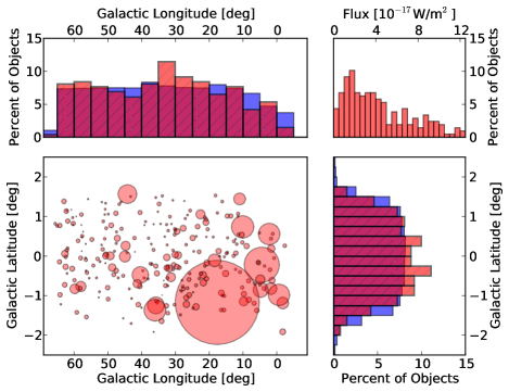
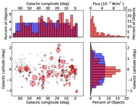
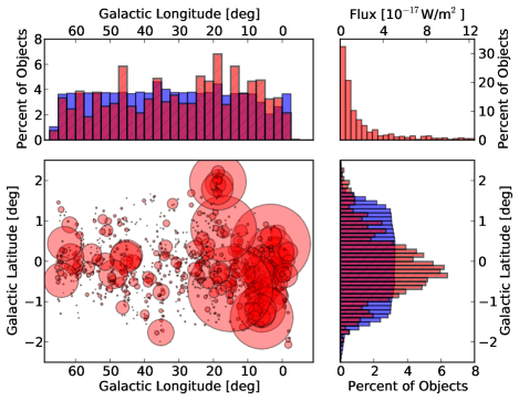
Figure 8: Distributions of PNe (top panel), jet groups (middle panel) and unknown objects (mostly PDRs, bottom panel). For each object type there are four plots. The bottom left indicates the spatial distribution where the circle size indicates the total flux of each group. The same scaling is applied in all plots. The top right graph show the distribution of the total fluxes for each group. Some of the bright groups of unknown objects are beyond the limit of the graph. The top left and bottom right graphs show the distribution of the number of objects along and across the GP (red, hatched) vs. the survey coverage (blue, unhatched).

In Fig. 8 we show the spatial distributions of all the groups of objects (Jets, PNe, unknown/PDR) as well as their flux distributions. The distributions along the GP show that the objects are distributed slightly differently. In particular they are not in agreement with a homogeneous distribution in our survey. The distribution indicates that there are slightly less PNe than expected for a homogeneous distribution at Galactic longitudes less than 20°– 30°. This is most likely due to the higher extinction in this direction which will lower our detection limit to smaller distances. This is further supported by Table 2 which indicates the number of PNe per unit area in the inner GP is about 10 % lower than in the outer GP. A KS-test shows that the PN longitude distribution has a 96.1 % chance of being drawn from a homogeneous distribution. The longitude distributions of the groups of Jets and unknown/PDR objects, both of them representing star forming regions, are clearly different. There is a clear overabundance of objects compared to a homogeneous distribution for longitudes of less than 30°. A KS-test shows that both distributions have a probability of only 1.4 % (Jets) and 3.0 % (unknown/PDR) to be drawn from a homogeneous sample. It is also evident that groups (of both Jets and unknown/PDR objects) within 30° of the GC are much brighter than the groups further away (see Table 2), indicating stronger star formation activity (traced in H₂ ) closer to the GC. Furthermore, the spatial distribution of the groups of Jets and PDRs is much more clustered than for the PNe. Hence, the small star forming groups follow the large scale filamentary structure of GMCs along the GP.

We also determined the scale height of the distribution of the objects perpendicular to the GP. We utilised the method developed by Buckner & Froebrich (2014) to obtain the scale height and zero point of a Galactic latitude distribution. For the PNe we find a scale height of 0^∘​​.92 $\pm$ 0^∘​​.11 with a zero point at $b$ $=$ $-$0^∘​​.01 $\pm$ 0^∘​​.01. However, due to our limited latitude coverage, this scale height should be taken as a lower limit. Indeed there is a 38.9 % KS-test probability that the distribution of PNe across the GP in our survey area is drawn from a homogeneously distributed sample. The vertical zero point of the PN distribution coincides (within the uncertainties) with the GP. This shows that the PNe trace an older, evolved population of objects. For the Jets and PDRs the scale heights are smaller with 0^∘​​.65 $\pm$ 0^∘​​.06 and 0^∘​​.66 $\pm$ 0^∘​​.04, respectively. The distribution zero points are at $-$0^∘​​.18 $\pm$ 0^∘​​.01 and $-$0^∘​​.17 $\pm$ 0^∘​​.01, respectively. Thus, within the uncertainties, the scale height and zero points of these distributions are identical, even if a KS-test gives only a 34.1 % probability that the vertical distributions of both groups are drawn from the same parent distribution. They hence trace the same component of the star formation process. The vertical zero points for groups of jets and unknown objects are significantly below the GP. This is in good agreement with them tracing active star formation, which coincides with the dust and young cluster distribution which is shifted below the GP in the longitude range of our survey (e.g. Drimmel et al. (2003), Marshall et al. (2006), Buckner & Froebrich (2014)).

4.2 Jets and Outflows, PDRs, Star Formation

We can use all the H₂  features which are classified as Jets or PDRs as indicators of star formation activity. Jets most commonly trace young, accreting protostars and/or Classical T-Tauri stars. Objects we have classified as PDRs are most likely excited by slightly more evolved young stars and are often found near clusters or intermediate mass stars.

Considering the respective survey areas, the Cygnus region clearly has the highest projected Jet/PDR group density. While along the GP there are on average about 2.15 Jet groups per square degree, in Cygnus the density is 5.00 per square degree. For PDRs there are 4.43 groups per square degree along the GP and 8.41 in Cygnus. This is most likely due to the fact that we specifically targeted high column density regions in Cygnus, i.e. active places of star formation. However, we used the same strategy in Auriga, which can be considered an example SF region in the outer GP, but we find on average only 1.44 Jet groups and 0.87 PDRs per square degree. This is a clear indication that the number of H₂  features is related to the general star formation activity which seems lowest in Auriga despite the bias in the survey. Furthermore, both SF indicators (Jets and PDRs) are clearly more prevalent in the inner GP compared to the outer GP.

A similar picture emerges if one uses the total flux of all features in each part of the survey to trace star formation activity. All the details are summarised in Table 1. The total H₂  flux per square degree from Jets is about 6.1 times higher in Cygnus compared to the GP. The flux per area for PDRs is 3.0 times higher in Cygnus than in the GP. In Auriga the flux per square degree from jets is 6.6 times lower than in the GP and for PDRs its 4.5 times lower. Thus, despite the focus on SF regions in the observations of Auriga, this region clearly stands out as the least active SF region in the survey.

We further investigate the median total fluxes for object groups, which we calculate by summing up the total fluxes of all H₂  features in the group and calculating the median over all groups (see Table 2). These fluxes can be considered as typical fluxes for each group of objects, as they are not influenced by extreme outliers (see e.g. the two extremely bright SNRs in Section 4.4). For Jet groups and PDRs these fluxes are generally lower in the outer GP than in the inner GP. For Jets the variations of the median total fluxes in the four sub-regions are less than a factor of a few, suggesting that the typical group of jets and outflows are similar in all the investigated regions and that extinction and distances to the typical Jet groups are comparable. Furthermore, the median total fluxes of the PDRs are very similar in the inner GP and Cygnus/Auriga, i.e. the typical SF regions in these areas are comparable in terms of their flux, but their numbers are highly variable.

In summary, the Jet and PDR features in the survey give a clear indication of the differences in the currently ongoing star formation activity (traced by H₂ ) in the areas covered by the survey. There are clearly more Jet groups and PDRs per unit area in the more active star forming regions but the individual objects are typically of a similar brightness. Please note that we cannot discuss any influences on the observed fluxes by systematic differences in distance and extinction to the typical objects observed in the various parts of the survey.

We are preparing more detailed investigations of the jets and outflows in Cygnus and Auriga. Several regions along the GP have also already been studied in detail (e.g. Ioannidis & Froebrich (2012a), Ioannidis & Froebrich (2012b), Froebrich & Ioannidis (2011), Lee et al. (2012), Dewangan et al. (2012), Lim et al. (2012), Dewangan & Ojha (2013), Lee et al. (2013), Dewangan et al. (2015), Dewangan et al. (2015)).

4.3 Planetary Nebulae

A list of groups of H₂  detections which coincide with known PNe or which we consider to be new PNe candidates is given in Table LABEL:pndatatable in the Appendix. We list the group/source ID (which contains the Galactic coordinates), Right Ascension and Declination, the radius of the circumscribing circle enclosing all detected H₂  emission, the area of emission, and the corresponding total and median fluxes. Finally, for previously known objects considered to be PNe, we give the PN G identifier where available. In cases where a known object is listed in SIMBAD but has not been identified as a PN then we give the alternative identifier (e.g. the IRAS name).

Approximately 60 % of the H₂  detections in Table LABEL:pndatatable correspond to emission features that have no corresponding source in SIMBAD and have not been identified as PN or PN candidates in the literature. We list these as New and have flagged them as possible PNe on the basis of their morphology and lack of association with known star formation activity. We stress that these are candidate PNe and their true nature will be established by follow-up observations (Gledhill et al. in prep.). These include two PNe candidates that have previously been identified as MHOs in (Ioannidis & Froebrich, 2012a).

The number of PNe per square degree is 1.25 for the GP, with 1.18 and 1.31 per square degree in the inner and outer GP regions respectively (defined as $-3\degr<l<30\degr$ and $30\degr\leq l<66\degr$). Interestingly, the higher space density in the outer GP arises from New detections; 58 % of H₂  detections in the inner GP are new, and 65 % in the outer GP, corresponding to 0.68 and 0.85 objects per square degree, respectively. By contrast, the density of previously known PNe (with PN G identifiers) which also have H₂  emission, is 0.34 per square degree in both regions.

The lower space density of PNe in the inner GP may be a consequence of increased extinction along these sightlines. This is further supported by the larger median flux for inner GP PNe ($570\times 10^{-19}$ W m^-2 compared with $366\times 10^{-19}$ W m^-2) suggesting that we are sampling shorter sightlines. However, the higher fraction of New H₂ -detected PNe in the outer, compared to inner GP (65 % compared to 58 %) indicates that we have not uncovered a population of inner-Galaxy PNe that were previously obscured in optical surveys. The Galactic distribution of H₂ -detected PNe shown in Fig. 8 is actually similar to that of optically detected IPHAS PNe (Sabin et al., 2014).

Table 3: List of SNRs with identified extended H₂  emission line features in our survey. The data (positions, size, type, 1 GHz flux, spectral index and other identifiers) are taken from Green (2014). The area covered by H₂  emission, the total and median fluxes as well as the number of individual H₂  emission regions are also listed. Note that G 6.5$-$0.4 also overlaps with several extended H₂  features. However, due to their visual appearance we attribute all of these to W 28.

Name	RA	DEC	Size	Area	1 GHz flux	spectral	Ftot	Fmed	number of	type	other
	(J2000)		[arcmin]	[arcmin2]	[Jy]	index	[10-15 W m-2]		regions		name
G1.0$-$0.1	17:48:30	$-$28:09	8	0.12	15	0.6?	0.24	0.22	4	S
G1.4$-$0.1	17:49:39	$-$27:46	10	0.076	2?	?	0.43	0.18	7	S
G5.5$+$0.3	17:57:04	$-$24:00	15x12	0.28	5.5	0.7	1.12	0.82	8	S
G6.1$+$0.5	17:57:29	$-$23:25	18x12	0.052	4.5	0.9	0.11	0.10	3	S
G6.4$-$0.1	18:00:30	$-$23:26	48	34.8	310	varies	126	89	1530	C	W 28
G9.9$-$0.8	18:10:41	$-$20:43	12	0.11	6.7	0.4	0.10	0.09	20	S
G11.2$-$0.3	18:11:27	$-$19:25	4	1.70	22	0.5	5.2	3.2	77	C
G13.5$+$0.2	18:14:14	$-$17:12	5x4	0.049	3.5?	1.0?	0.06	0.05	6	S
G16.0$-$0.5	18:21:56	$-$15:14	15x10	0.40	2.7	0.6	1.6	0.54	47	S
G18.1$-$0.1	18:24:34	$-$13:11	8	0.34	4.6	0.5	3.0	0.92	48	S
G18.9$-$1.1	18:29:50	$-$12:58	33	0.80	37	0.39	1.1	0.97	102	C?
G21.6$-$0.8	18:33:40	$-$10:25	13	0.020	1.4	0.5?	0.02	0.02	5	S
G21.8$-$0.6	18:32:45	$-$10:08	20	1.75	65	0.56	4.3	3.7	119	S	Kes 69
G24.7$+$0.6	18:34:10	$-$07:05	30x15	0.42	20?	0.2?	0.48	0.44	70	C?
G27.4$+$0.0	18:41:19	$-$04:56	4	0.054	6	0.68	0.09	0.09	9	S	4C$-$04.71
G27.8$+$0.6	18:39:50	$-$04:24	50x30	0.11	30	varies	0.15	0.14	3	F
G28.8$+$1.5	18:39:00	$-$02:55	100?	0.046	?	0.4?	0.04	0.04	7	S?
G31.9$+$0.0	18:49:25	$-$00:55	7x5	2.32	25	varies	15.6	7.2	102	S	3C391
G32.1$-$0.9	18:53:10	$-$01:08	40?	0.55	?	?	1.8	0.70	71	C?
G32.8$-$0.1	18:51:25	$-$00:08	17	2.20	11?	0.2?	7.5	2.9	203	S?	Kes 78
G33.2$-$0.6	18:53:50	$-$00:02	18	0.12	3.5	varies	0.71	0.17	12	S
G34.7$-$0.4	18:56:00	$+$01:22	35x27	62.9	250	0.37	263	157	2852	C	W 44
G38.7$-$1.3	19:06:40	$+$04:28	32x19?	0.26	?	?	0.57	0.29	43	S
G39.2$-$0.3	19:04:08	$+$05:28	8x6	0.52	18	0.34	0.75	0.70	49	C	3C396
G43.3$-$0.2	19:11:08	$+$09:06	4x3	5.0	38	0.46	15.5	13.7	107	S	W 49B
G54.4$-$0.3	19:33:20	$+$18:56	40	0.39	28	0.5	0.52	0.41	54	S	HC 40
G65.1$+$0.6	19:54:40	$+$28:35	90x50	0.13	5.5	0.61	0.06	0.09	7	S
G357.7$+$0.3	17:38:35	$-$30:44	24	0.032	10	0.4?	0.09	0.08	2	S
G359.0$-$0.9	17:46:50	$-$30:16	23	0.15	23	0.5	0.30	0.30	10	S
G359.1$-$0.5	17:45:30	$-$29:57	24	1.31	14	0.4?	10.3	3.3	53	S

4.4 Supernova Remnants

There are about 300 known SNRs in the Milky Way (Green, 2014), and 119 SNRs are either fully or partially covered in the UWISH2 survey, including seven SNRs in Cygnus and one SNR in Auriga. We have detected H₂  emission features which are most likely associated with SNRs for 30 of them. Hence, the H₂  SNR detection rate is 25 %. Table 3 lists the SNRs with H₂  emission features where we list the SNR name, coordinates, sizes, types and other names. All parameters in this Table (except area covered in H₂  and fluxes) are from Green (2014). Please note that the SNR G6.5$-$0.4 also overlaps with several extended H₂  features. However, due to their visual appearance we attribute all of these to the larger, more extended SNR W 28.

The SNRs bright in H₂  emission in Table 3, e.g., W 28, 3C391, W 44, and W 49B, are prototypical SNRs interacting with molecular clouds. In these SNRs, the H₂  features fall on bright radio filaments, where the SN blast wave might be encountering dense environment. These H₂  emission features are probably shock excited. In some SNRs, however, H₂  features are just outside the radio continuum boundary (e.g. in G 11.2$-$0.3), and those features could be radiatively excited (Koo, 2014). Note that W 44 and W 28 are responsible for 84 % of the total H₂  emission associated with SNRs in our survey (57 % and 27 %, respectively). A much more detailed discussion of the H₂  emission features associated with SNRs will be presented in a forthcoming paper (Lee et al. 2015, in preparation).

5 Conclusions

We have used WFCAM at UKIRT to conduct a large survey for emission of the H₂  1 – 0 S(1) line at 2.122 $\mu$m. An unbiased survey along the GP from $l\approx 357\degr$ to $l\approx 65\degr$ and $|b|\leq$ 1^∘​​.5 covers about 209 square degrees. We have further targeted high column density areas in Cygnus (42.0 square degrees) and Auriga (35.5 square degrees).

We have compiled a catalogue of extended H₂  emission line features in this survey. All features were automatically detected and manually verified. We estimate that only 1 – 2 % of the objects in the catalogue are false positives and that 95 % of the real automatic detections are in the final catalogue. Mostly small features in the vicinity of larger extended H₂  emission might be missing but these do not contribute with any significance to the total detected H₂  flux. All features are also manually classified as either part of a Jet/outflow, PN or SNR. All other objects are unclassified but these are most likely part of PDRs.

In total, 33200 individual extended H₂  emission line features are contained in our catalogue. There are about 700 groups of jet/outflow features, 284 PNe, 30 SNRs and about 1300 groups of PDRs. The total H₂  flux is dominated by the PDR and SNR features (each accounting for 40 – 45 % of all the flux). The Jet groups and PNe each contain about 7 – 9 % of the flux.

We find that star formation (traced by H₂  emission of Jets and PDRs) is strongest in the inner GP (less than 30° from the Galactic Centre) and in the Cygnus region. The latter containing, due to our targeted survey, the highest number of Jet or PDR groups per square degree. Auriga clearly shows the lowest star formation activity based on all our measures (density of sources, total H₂  flux etc.) and there is also a clear decline in the star formation activity with distance from the Galactic Centre.

About 60 % of all the PNe and candidate PNe in our catalogue have no known counterpart in any of the PNe catalogues. Hence our survey has uncovered a significant, unknown population of young and or embedded PNe candidates in the GP. Their spatial distribution, however, is very similar to the optically detected PNe.

Of all SNRs (partially) covered by our survey, one quarter has detectable H₂   emission. The total flux in these H₂  features is strongly dominated by W 44 and W 28 which together contain 84 % of all the H₂  flux associated with SNRs.

Appendix A map$\_$zp distributions

Appendix B Properties of PNe

Table 4: Table listing all the PNe detected in our survey. We list the UWISH2 PN source ID, which includes the Galactic coordinates, the RA and DEC (J2000) positions of the geometric centre of the H₂  emitting features in the PN, the radius around this central position enclosing all the H₂  emission, the area covered with H₂  emission, the total and median fluxes of the PN, and any other known name/identifier or coinciding object (not necessarily a PN). ’New’ in the last column indicates objects that have so far not been recognised as PNe or PNe candidates in the literature.

Source ID	RA	DEC	Radius	Area	Ftot	Fmed	Other ID
	[deg]	[deg]	[arcsec]	[arcsec2]	[10-19Wm-2]
PN$\_$UWISH2$\_$000.81878$-$0.04944	266.93718	$-$28.26207	6.3	52.97	388.50	345.89	SSTGC 841071
PN$\_$UWISH2$\_$001.22588$+$0.56414	266.58223	$-$27.59584	5.7	44.18	386.74	331.79	New
PN$\_$UWISH2$\_$001.42213$-$0.61357	267.83773	$-$28.03457	16.9	243.11	1706.78	1796.58	New
PN$\_$UWISH2$\_$001.65056$+$0.18803	267.19290	$-$27.42713	14.8	298.48	2544.15	2286.36	PN G001.6$+$00.1
PN$\_$UWISH2$\_$001.72196$-$0.82262	268.21435	$-$27.88315	17.3	211.92	6355.37	1543.66	New
PN$\_$UWISH2$\_$001.73118$+$0.44232	266.99457	$-$27.22684	12.2	137.19	498.93	439.01	New
PN$\_$UWISH2$\_$002.03824$-$0.34363	267.93092	$-$27.36701	23.4	149.54	680.57	655.32	New
PN$\_$UWISH2$\_$002.25319$+$0.55724	267.18642	$-$26.72043	47.7	1312.63	1712.21	9032.45	PN G002.2$+$00.5
PN$\_$UWISH2$\_$003.65197$-$0.25068	268.75783	$-$25.92948	4.9	48.46	323.03	309.66	New
PN$\_$UWISH2$\_$003.79367$-$0.81428	269.37918	$-$26.09041	5.7	35.84	746.92	224.72	New
PN$\_$UWISH2$\_$004.44847$-$0.21905	269.17220	$-$25.22542	88.9	2267.66	7638.52	18397.78	New
PN$\_$UWISH2$\_$004.76799$-$0.85257	269.95542	$-$25.26527	17.1	289.48	0582.35	2023.47	New
PN$\_$UWISH2$\_$004.88887$-$0.58981	269.77016	$-$25.02963	38.6	690.14	3875.28	3181.93	PN G004.8$-$00.5
PN$\_$UWISH2$\_$004.99841$-$0.72107	269.95596	$-$24.99999	6.5	60.86	338.48	306.73	New
PN$\_$UWISH2$\_$005.14078$+$0.58616	268.79000	$-$24.22186	6.5	40.10	205.82	202.82	New
PN$\_$UWISH2$\_$005.42811$-$0.16852	269.66434	$-$24.35213	26.1	178.42	906.42	848.62	New
PN$\_$UWISH2$\_$005.56222$-$0.15023	269.72037	$-$24.22679	10.5	112.38	478.75	485.48	New
PN$\_$UWISH2$\_$005.90685$-$1.37325	271.07450	$-$24.53226	17.8	279.37	992.38	1008.53	New
PN$\_$UWISH2$\_$006.51856$-$0.69279	270.75465	$-$23.66517	8.5	96.85	425.90	405.80	New
PN$\_$UWISH2$\_$006.73073$-$1.19177	271.34313	$-$23.72525	11.0	169.83	829.38	765.93	New
PN$\_$UWISH2$\_$008.33574$-$1.10291	272.10781	$-$22.28043	19.1	109.88	1414.41	551.62	PN G008.3$-$01.1
PN$\_$UWISH2$\_$008.36142$-$0.62384	271.66930	$-$22.02504	8.9	112.93	794.42	606.43	IRAS 18036$-$2201
PN$\_$UWISH2$\_$008.94169$+$0.25318	271.15183	$-$21.09003	15.7	205.01	1280.44	1158.31	MGE G008.9409$+$00.2532
PN$\_$UWISH2$\_$009.76150$-$0.95756	272.71231	$-$20.96230	10.7	143.92	1308.31	761.34	SSTGLMC G009.7612$-$00.9575
PN$\_$UWISH2$\_$009.80708$-$1.14613	272.91283	$-$21.01314	20.9	376.92	3534.44	3056.88	PN G009.8$-$01.1
PN$\_$UWISH2$\_$010.10373$+$0.73752	271.30883	$-$19.83976	110.7	2993.26	23449.28	20473.46	PN G010.1$+$00.7
PN$\_$UWISH2$\_$010.21147$+$0.34469	271.72932	$-$19.93758	30.7	190.12	571.03	555.52	PN G010.2$+$00.3
PN$\_$UWISH2$\_$010.26120$-$0.79452	272.81690	$-$20.44591	8.0	132.78	537.11	512.53	New
PN$\_$UWISH2$\_$010.39239$+$0.53966	271.64211	$-$19.68458	20.1	301.02	1239.45	1159.96	SSTGLMC G010.393$+$00.538
PN$\_$UWISH2$\_$010.94194$-$0.40277	272.80040	$-$19.66068	13.2	133.56	435.56	422.76	New
PN$\_$UWISH2$\_$011.00185$+$1.44395	271.12230	$-$18.71089	18.7	503.97	6480.38	3915.85	PN G011.0$+$01.4
PN$\_$UWISH2$\_$011.32982$+$0.54981	272.11575	$-$18.86062	7.4	98.14	360.27	424.95	New
PN$\_$UWISH2$\_$011.45829$+$1.07349	271.69860	$-$18.49376	4.0	49.55	455.05	345.22	IRAS 18038$-$1830
PN$\_$UWISH2$\_$011.52915$+$1.00385	271.79911	$-$18.46579	8.2	72.03	181.51	188.48	PN G011.5$+$01.0
PN$\_$UWISH2$\_$011.86338$+$0.30190	272.61733	$-$18.51366	6.0	67.67	292.62	280.15	New
PN$\_$UWISH2$\_$012.11515$+$0.07516	272.95467	$-$18.40229	12.3	179.10	899.29	872.22	GPSR5 12.116$+$0.076
PN$\_$UWISH2$\_$012.20907$+$0.43081	272.67407	$-$18.14868	5.2	36.29	93.15	87.46	New
PN$\_$UWISH2$\_$012.21971$-$0.33477	273.38671	$-$18.50730	10.8	67.23	241.45	198.28	New
PN$\_$UWISH2$\_$012.71728$+$0.37202	272.98548	$-$17.73160	7.6	105.71	403.04	372.10	New
PN$\_$UWISH2$\_$012.80348$+$0.00510	273.36698	$-$17.83207	16.9	144.48	463.28	427.44	New
PN$\_$UWISH2$\_$013.61090$+$1.01274	272.84745	$-$16.64001	9.2	145.48	820.75	699.76	New
PN$\_$UWISH2$\_$014.58523$+$0.46161	273.83795	$-$16.04881	7.4	56.81	247.96	213.56	PN G014.5$+$00.4
PN$\_$UWISH2$\_$014.64501$+$0.08920	274.20847	$-$16.17352	10.4	85.77	317.09	321.64	New
PN$\_$UWISH2$\_$014.65833$+$1.01220	273.37138	$-$15.72154	18.8	186.94	887.33	882.35	PN G014.6$+$01.0
PN$\_$UWISH2$\_$014.92112$+$0.06989	274.36260	$-$15.93970	17.5	101.11	384.56	385.95	IRAS 18145$-$1557
PN$\_$UWISH2$\_$015.13012$-$0.44046	274.93310	$-$15.99718	30.5	368.79	1810.59	1662.43	New
PN$\_$UWISH2$\_$015.53753$-$0.01923	274.74746	$-$15.43907	29.9	43.62	189.24	178.44	PN G015.5$-$00.0
PN$\_$UWISH2$\_$015.54859$-$1.00657	275.65740	$-$15.89444	8.5	73.78	414.18	379.23	IRAS 18197$-$1555
PN$\_$UWISH2$\_$015.67993$-$1.36320	276.04901	$-$15.94546	11.4	150.86	693.24	629.09	New
PN$\_$UWISH2$\_$016.02790$-$1.00525	275.88952	$-$15.47051	4.7	41.72	152.10	146.44	New
PN$\_$UWISH2$\_$016.11984$-$0.98789	275.91826	$-$15.38115	16.6	110.13	255.34	259.28	New
PN$\_$UWISH2$\_$016.17480$+$1.37914	273.78738	$-$14.21429	12.5	114.53	345.46	350.14	New
PN$\_$UWISH2$\_$016.41571$-$0.93047	276.00920	$-$15.09285	32.3	326.45	1539.81	1349.89	PN G016.4$-$00.9
PN$\_$UWISH2$\_$016.48834$-$1.36082	276.43858	$-$15.22966	33.8	188.83	570.06	557.68	New
PN$\_$UWISH2$\_$016.60078$-$0.27565	275.50065	$-$14.62230	8.5	101.08	461.29	411.40	New
PN$\_$UWISH2$\_$016.92321$-$0.00616	275.41159	$-$14.21103	6.7	64.19	185.62	179.73	New
PN$\_$UWISH2$\_$017.22288$+$0.12645	275.43624	$-$13.88420	37.3	232.61	1324.38	790.29	PN G017.2$+$00.1
PN$\_$UWISH2$\_$017.58861$+$1.09048	274.73927	$-$13.10716	7.8	72.61	282.56	256.31	New
PN$\_$UWISH2$\_$017.61528$-$1.17013	276.80657	$-$14.14383	152.8	6864.53	330258.97	85111.55	PN G017.6$-$01.1
PN$\_$UWISH2$\_$018.14941$+$1.53214	274.61205	$-$12.40431	9.9	73.37	356.23	285.41	PN G018.1$+$01.5
PN$\_$UWISH2$\_$018.41760$-$0.10793	276.22489	$-$12.93880	14.8	250.57	7524.71	1420.73	New
PN$\_$UWISH2$\_$018.83207$+$0.48278	275.88871	$-$12.29607	3.6	29.65	193.62	182.94	New
PN$\_$UWISH2$\_$020.46958$+$0.67836	276.49348	$-$10.75715	31.0	144.90	497.17	474.42	PN G020.4$+$00.6
PN$\_$UWISH2$\_$020.70907$-$0.17267	277.37398	$-$10.94099	12.9	261.67	1516.99	1431.33	New
PN$\_$UWISH2$\_$020.80590$-$0.57267	277.78078	$-$11.04048	16.4	202.93	898.55	855.13	New
PN$\_$UWISH2$\_$020.85450$+$0.48588	276.84922	$-$10.50625	2.4	10.67	108.07	67.97	SSTGLMC G020.8543$+$00.4857
PN$\_$UWISH2$\_$020.97795$+$0.92363	276.51391	$-$10.19310	28.1	137.21	684.15	592.45	GPSR 020.979$+$0.925
PN$\_$UWISH2$\_$020.98141$+$0.85244	276.57954	$-$10.22323	25.7	293.44	1726.19	1527.14	MHO 3200
PN$\_$UWISH2$\_$021.29383$+$0.98091	276.61194	$-$9.88697	9.6	109.65	417.59	382.68	PN G021.2$+$00.9
PN$\_$UWISH2$\_$021.30767$-$0.25089	277.72679	$-$10.44677	22.0	103.42	303.70	295.95	New
PN$\_$UWISH2$\_$021.74338$-$0.67287	278.31186	$-$10.25536	14.0	211.85	1983.87	1480.83	PN G021.7$-$00.6
PN$\_$UWISH2$\_$021.81951$-$0.47837	278.17225	$-$10.09807	26.3	429.56	2257.37	2074.66	PN G021.8$-$00.4
PN$\_$UWISH2$\_$022.44734$-$0.44228	278.43371	$-$9.52442	25.3	165.39	608.36	580.98	New
PN$\_$UWISH2$\_$022.57000$+$1.05505	277.14674	$-$8.72291	13.1	289.63	3901.84	3278.61	PN G022.5$+$01.0
PN$\_$UWISH2$\_$022.99501$-$0.56968	278.80394	$-$9.09703	7.8	83.05	255.30	243.34	New
PN$\_$UWISH2$\_$022.99982$+$0.10714	278.19818	$-$8.78078	22.7	183.99	666.78	624.85	New
PN$\_$UWISH2$\_$023.44011$+$0.74528	277.83172	$-$8.09545	10.4	160.99	996.94	898.32	PN G023.4$+$00.7
PN$\_$UWISH2$\_$023.78286$+$0.50238	278.20917	$-$7.90372	3.5	23.67	126.19	106.99	New
PN$\_$UWISH2$\_$023.89021$-$0.73778	279.37125	$-$8.37930	12.8	158.79	426.44	567.42	GPSR 023.890$-$0.737
PN$\_$UWISH2$\_$023.90016$-$1.28024	279.86330	$-$8.61917	13.6	238.74	1905.40	1258.16	PN G023.9$-$01.2
PN$\_$UWISH2$\_$024.58540$+$0.11989	278.92479	$-$7.36772	7.8	43.53	162.26	138.43	New
PN$\_$UWISH2$\_$024.76272$-$0.91396	279.93336	$-$7.68478	2.8	16.29	110.21	97.41	New
PN$\_$UWISH2$\_$024.77483$-$1.31616	280.29988	$-$7.85808	41.4	93.54	261.05	256.44	MHO 2456
PN$\_$UWISH2$\_$024.89596$+$0.45853	278.76581	$-$6.93617	9.2	118.28	341.25	891.83	G024.8959$+$00.4586
PN$\_$UWISH2$\_$025.66408$+$1.15020	278.50388	$-$5.93589	28.4	151.60	402.43	414.26	PN G025.6$+$01.1
PN$\_$UWISH2$\_$025.77993$-$0.44005	279.97837	$-$6.56355	4.1	37.20	284.64	231.01	New
PN$\_$UWISH2$\_$025.92671$-$0.98449	280.53333	$-$6.68220	10.0	106.93	1165.94	857.58	PN G025.9$-$00.9
PN$\_$UWISH2$\_$025.99096$-$0.59183	280.21143	$-$6.44546	5.5	116.81	730.31	685.15	New
PN$\_$UWISH2$\_$026.42837$+$1.03759	278.95767	$-$5.30927	5.2	35.20	144.32	124.96	New
PN$\_$UWISH2$\_$026.44767$-$0.80840	280.61536	$-$6.13843	7.6	74.54	374.88	348.10	New
PN$\_$UWISH2$\_$026.74999$-$1.21865	281.12124	$-$6.05692	12.8	308.77	1998.37	1713.67	PN G026.7$-$01.2
PN$\_$UWISH2$\_$026.79572$-$1.05024	280.99156	$-$5.93937	13.2	201.09	1233.94	1023.55	PN G026.8$-$01.0
PN$\_$UWISH2$\_$026.83269$-$0.15180	280.20553	$-$5.49569	6.9	66.40	490.11	436.91	PN G026.8$-$00.1
PN$\_$UWISH2$\_$026.83640$+$0.28828	279.81431	$-$5.29077	4.9	42.57	316.53	310.34	New
PN$\_$UWISH2$\_$027.09954$+$0.94886	279.34624	$-$4.75395	6.8	75.15	233.94	226.95	New
PN$\_$UWISH2$\_$027.37280$+$1.39262	279.07660	$-$4.30750	4.1	21.17	60.48	62.66	New
PN$\_$UWISH2$\_$027.66357$-$0.82670	281.18977	$-$5.06529	11.7	137.45	664.66	598.03	PN G027.6$-$00.8
PN$\_$UWISH2$\_$027.70327$+$0.70354	279.84264	$-$4.33003	37.4	386.40	1632.32	1556.50	PN G027.7$+$00.7
PN$\_$UWISH2$\_$027.81843$-$0.76628	281.20679	$-$4.89994	7.1	56.83	318.47	289.26	PN G027.8$-$00.7
PN$\_$UWISH2$\_$028.06295$-$0.61048	281.17972	$-$4.61128	4.9	34.62	137.77	132.94	New
PN$\_$UWISH2$\_$028.19767$-$0.89109	281.49190	$-$4.61951	11.7	61.46	164.11	161.12	New
PN$\_$UWISH2$\_$028.52225$-$1.48422	282.16994	$-$4.60108	30.4	99.29	274.33	277.01	PN G028.5$-$01.4
PN$\_$UWISH2$\_$028.62122$-$0.86537	281.66273	$-$4.23091	7.7	29.57	63.90	65.83	New
PN$\_$UWISH2$\_$028.89451$-$0.29151	281.27590	$-$3.72585	32.6	202.61	780.88	762.12	PN G028.8$-$00.2
PN$\_$UWISH2$\_$029.21554$+$0.02262	281.14282	$-$3.29679	22.0	215.51	2369.65	711.76	New
PN$\_$UWISH2$\_$029.50204$+$0.62395	280.73827	$-$2.76719	15.6	316.05	1600.87	1607.46	PN G029.5$+$00.6
PN$\_$UWISH2$\_$029.57883$-$0.26901	281.56882	$-$3.10673	6.1	49.36	258.66	660.93	PN G029.5$-$00.2
PN$\_$UWISH2$\_$029.99765$+$0.65621	280.93623	$-$2.31163	5.6	55.76	351.46	325.64	G30.421$-$0.226
PN$\_$UWISH2$\_$030.04497$+$0.03465	281.51132	$-$2.55337	31.1	452.87	1929.37	1880.83	PN G030.0$+$00.0
PN$\_$UWISH2$\_$030.17049$+$0.68782	280.98710	$-$2.14346	5.9	54.68	356.97	300.21	New
PN$\_$UWISH2$\_$030.22594$+$0.54285	281.14150	$-$2.16034	14.0	108.68	414.40	398.18	New
PN$\_$UWISH2$\_$030.30097$-$1.22812	282.75329	$-$2.90143	9.0	78.48	351.91	292.73	New
PN$\_$UWISH2$\_$030.50743$-$0.21913	281.94856	$-$2.25769	17.0	199.62	943.44	847.33	PN G030.5$-$00.2
PN$\_$UWISH2$\_$030.66759$-$0.33136	282.12162	$-$2.16634	11.7	76.83	399.40	322.69	G030.6671$-$00.3316
PN$\_$UWISH2$\_$030.72160$+$0.14788	281.71954	$-$1.89964	14.9	100.07	270.46	280.51	New
PN$\_$UWISH2$\_$030.76828$+$1.40983	280.61768	$-$1.28196	3.7	24.77	126.92	114.19	New
PN$\_$UWISH2$\_$031.16908$+$0.81029	281.33422	$-$1.19919	3.3	22.97	95.06	90.50	New
PN$\_$UWISH2$\_$031.32618$-$0.53286	282.60153	$-$1.67212	44.9	592.19	3797.09	3019.22	PN G031.3$-$00.5
PN$\_$UWISH2$\_$031.63781$+$0.99595	281.38290	$-$0.69744	6.6	62.40	389.78	344.45	New
PN$\_$UWISH2$\_$031.90685$-$0.30936	282.66738	$-$1.05343	27.7	368.30	2400.90	2183.65	PN G031.9$-$00.3
PN$\_$UWISH2$\_$032.14993$+$0.64445	281.92933	$-$0.40212	7.6	62.99	300.67	251.96	New
PN$\_$UWISH2$\_$032.22860$-$1.44045	283.82102	$-$1.28266	30.1	211.09	597.61	614.37	PN G032.2$-$01.4
PN$\_$UWISH2$\_$032.28479$-$0.27816	282.81195	$-$0.70284	7.2	91.60	477.47	438.76	New
PN$\_$UWISH2$\_$032.29224$-$0.74568	283.23149	$-$0.90936	4.1	29.38	231.96	173.05	New
PN$\_$UWISH2$\_$032.37721$-$0.55490	283.10042	$-$0.74677	7.6	79.64	444.97	406.96	PN G032.3$-$00.5
PN$\_$UWISH2$\_$032.46866$+$0.28147	282.39772	$-$0.28401	6.6	53.49	199.32	171.17	New
PN$\_$UWISH2$\_$032.54650$-$0.03210	282.71230	$-$0.35773	17.9	281.26	2062.73	1760.69	PN G032.5$-$00.0
PN$\_$UWISH2$\_$032.54998$-$0.29529	282.94812	$-$0.47464	12.5	219.21	1571.41	1552.01	PN G032.5$-$00.3
PN$\_$UWISH2$\_$032.61348$+$0.79678	282.00515	$+$0.07986	3.8	31.65	241.38	160.47	PN PM 1$-$258
PN$\_$UWISH2$\_$032.66916$-$1.25559	283.85720	$-$0.80638	10.2	124.80	973.71	817.44	PN G032.6$-$01.2
PN$\_$UWISH2$\_$032.94004$-$0.74662	283.52766	$-$0.33328	7.9	102.73	759.84	697.54	PN G032.9$-$00.7
PN$\_$UWISH2$\_$033.16509$+$0.49150	282.52836	$+$0.43156	3.8	25.56	106.84	108.63	New
PN$\_$UWISH2$\_$033.45470$-$0.61500	283.64519	$+$0.18474	4.8	24.37	27.24	76.77	PN G033.4$-$00.6
PN$\_$UWISH2$\_$033.88796$+$1.52134	281.94106	$+$1.54427	33.8	86.69	255.42	247.80	PN G033.8$+$01.5
PN$\_$UWISH2$\_$033.97946$-$0.98557	284.21432	$+$0.48266	2.2	4.42	8.03	8.88	PN G033.9$-$00.9
PN$\_$UWISH2$\_$034.10462$-$1.64333	284.85672	$+$0.29388	12.0	148.05	1176.28	1034.87	PN G034.1$-$01.6
PN$\_$UWISH2$\_$034.41021$+$0.81477	282.80828	$+$1.68706	4.5	36.56	115.32	110.41	New
PN$\_$UWISH2$\_$034.84509$+$1.31721	282.55901	$+$2.30305	9.1	125.35	698.43	611.71	New
PN$\_$UWISH2$\_$035.18522$+$1.12134	282.88860	$+$2.51653	11.5	43.14	107.63	103.53	New
PN$\_$UWISH2$\_$035.23366$-$1.13623	284.92089	$+$1.52961	30.0	120.64	251.39	255.44	New
PN$\_$UWISH2$\_$035.38919$-$1.17506	285.02650	$+$1.65019	12.0	122.81	375.93	372.11	New
PN$\_$UWISH2$\_$035.47394$-$0.43716	284.40844	$+$2.06260	20.9	292.90	1251.38	1039.51	IRAS 18551$+$0159
PN$\_$UWISH2$\_$035.76967$-$1.24531	285.26293	$+$1.95644	16.6	461.29	3353.90	2827.71	New
PN$\_$UWISH2$\_$035.81426$+$1.48019	282.85558	$+$3.23983	11.8	75.27	181.05	183.03	New
PN$\_$UWISH2$\_$035.81489$-$0.25181	284.39919	$+$2.45055	15.6	279.99	850.69	834.37	New
PN$\_$UWISH2$\_$035.89918$-$1.14425	285.23222	$+$2.11780	4.9	44.77	196.69	182.66	New
PN$\_$UWISH2$\_$036.05309$-$1.36593	285.49991	$+$2.15329	149.5	4344.13	22362.90	20233.61	PN G035.9$-$01.1
PN$\_$UWISH2$\_$036.43225$-$1.91396	286.16112	$+$2.23949	1.7	4.02	58.24	30.95	PN G036.4$-$01.9
PN$\_$UWISH2$\_$036.46081$+$0.80581	283.75199	$+$3.50792	10.5	47.01	71.59	73.22	New
PN$\_$UWISH2$\_$036.48189$+$0.15610	284.34075	$+$3.23021	8.9	98.54	440.57	369.52	New
PN$\_$UWISH2$\_$036.98479$-$0.20330	284.89114	$+$3.51340	7.2	106.23	311.99	290.01	New
PN$\_$UWISH2$\_$037.14125$+$0.30341	284.51110	$+$3.88408	6.8	55.62	138.70	135.16	New
PN$\_$UWISH2$\_$037.41544$-$0.19254	285.07885	$+$3.90133	5.0	55.13	365.57	311.48	New
PN$\_$UWISH2$\_$037.96134$+$0.45337	284.75297	$+$4.68210	7.2	50.18	257.08	243.87	MSX6C G037.9595$+$00.4535
PN$\_$UWISH2$\_$038.14463$-$0.57489	285.75429	$+$4.37465	6.5	66.25	255.38	257.05	New
PN$\_$UWISH2$\_$038.83959$+$0.87057	284.78315	$+$5.65389	5.5	51.95	200.06	197.93	New
PN$\_$UWISH2$\_$039.16222$+$0.78375	285.00892	$+$5.90117	7.1	24.74	54.26	45.90	New
PN$\_$UWISH2$\_$039.26101$-$0.55123	286.24689	$+$5.37758	13.8	100.73	252.46	253.89	New
PN$\_$UWISH2$\_$039.64158$-$0.36822	286.25902	$+$5.79968	4.3	37.29	208.89	170.42	New
PN$\_$UWISH2$\_$040.03148$-$1.30313	287.27361	$+$5.71599	29.0	42.09	86.46	82.29	GPSR 040.033$-$1.302
PN$\_$UWISH2$\_$040.36950$-$0.47517	286.69085	$+$6.39710	32.2	1195.79	2682.48	9475.86	PN G040.3$-$00.4
PN$\_$UWISH2$\_$040.47073$+$1.10067	285.32726	$+$7.20967	7.6	76.14	797.05	546.69	New
PN$\_$UWISH2$\_$040.53948$-$0.76310	287.02679	$+$6.41554	8.0	144.08	050.63	1022.97	New
PN$\_$UWISH2$\_$040.96700$-$1.22601	287.63857	$+$6.58146	61.5	382.13	1021.97	1026.43	New
PN$\_$UWISH2$\_$041.27043$-$0.69797	287.30768	$+$7.09423	16.3	405.50	3270.84	2883.10	PN G041.2$-$00.6
PN$\_$UWISH2$\_$041.99634$+$0.10743	286.92389	$+$8.10956	19.9	16.17	24.70	26.29	New
PN$\_$UWISH2$\_$042.12631$+$0.45706	286.67062	$+$8.38580	9.0	126.16	547.41	509.69	New
PN$\_$UWISH2$\_$042.97101$-$1.07103	288.43505	$+$8.42942	4.9	38.11	152.55	146.72	New
PN$\_$UWISH2$\_$043.10420$-$1.70207	289.06236	$+$8.25419	9.8	68.68	172.42	174.90	New
PN$\_$UWISH2$\_$043.25830$+$1.50423	286.25472	$+$9.87206	5.5	40.78	191.80	134.57	New
PN$\_$UWISH2$\_$043.65562$-$0.82777	288.53841	$+$9.14866	4.0	39.85	194.97	196.86	New
PN$\_$UWISH2$\_$044.18877$+$1.56732	286.63144	$+$10.72749	100.4	1127.24	16445.03	2750.69	PN G044.1$+$01.5
PN$\_$UWISH2$\_$044.34714$+$0.08637	288.04202	$+$10.18518	6.1	73.84	187.67	177.95	New
PN$\_$UWISH2$\_$044.73433$+$0.26046	288.06742	$+$10.60898	16.1	325.33	3884.71	3071.11	PN G044.7$+$00.2
PN$\_$UWISH2$\_$044.93245$-$0.01060	288.40523	$+$10.65887	27.7	859.52	5722.84	4532.10	PN G044.9$+$00.0
PN$\_$UWISH2$\_$045.44425$-$1.57085	290.05177	$+$10.38386	11.0	50.65	83.50	84.33	New
PN$\_$UWISH2$\_$045.45878$-$0.49801	289.09365	$+$10.89817	31.3	186.85	443.03	433.85	New
PN$\_$UWISH2$\_$045.95707$+$0.69049	288.25641	$+$11.89176	21.8	192.00	504.54	445.28	New
PN$\_$UWISH2$\_$046.09523$+$1.36603	287.70922	$+$12.32673	5.8	53.80	157.90	140.96	New
PN$\_$UWISH2$\_$046.63335$+$1.31220	288.01280	$+$12.77895	6.8	90.48	323.00	294.06	New
PN$\_$UWISH2$\_$046.93735$-$0.54973	289.84548	$+$12.18115	5.4	43.42	204.57	180.63	New
PN$\_$UWISH2$\_$047.18522$+$0.44999	289.05872	$+$12.86745	14.3	367.10	1724.42	1558.36	New
PN$\_$UWISH2$\_$047.44521$+$0.61199	289.03591	$+$13.17296	5.8	70.25	212.27	191.78	New
PN$\_$UWISH2$\_$047.50612$-$0.36750	289.95370	$+$12.76896	15.1	188.00	982.46	827.20	New
PN$\_$UWISH2$\_$047.52536$+$0.32144	289.33823	$+$13.10836	7.5	68.59	245.39	244.87	New
PN$\_$UWISH2$\_$047.61228$+$1.08168	288.68845	$+$13.53933	11.4	212.69	926.61	903.93	PN G047.6$+$01.0
PN$\_$UWISH2$\_$048.03497$+$0.12296	289.76335	$+$13.46599	7.1	73.77	205.19	185.16	New
PN$\_$UWISH2$\_$048.24968$-$0.46947	290.40474	$+$13.37742	12.3	152.83	747.66	539.49	New
PN$\_$UWISH2$\_$048.71570$-$0.28960	290.46721	$+$13.87323	25.4	364.39	2620.46	2407.63	PN G048.7$-$00.2
PN$\_$UWISH2$\_$048.99884$+$0.77703	289.63259	$+$14.62389	16.9	240.14	1116.38	1035.00	New
PN$\_$UWISH2$\_$049.28561$+$0.00740	290.47382	$+$14.51586	46.3	569.06	2981.11	2487.01	PN G049.2$+$00.0
PN$\_$UWISH2$\_$049.86763$+$1.06075	289.79393	$+$15.52434	18.8	88.86	197.54	208.44	New
PN$\_$UWISH2$\_$049.91632$-$1.08675	291.77791	$+$14.55322	7.5	93.90	684.22	413.16	New
PN$\_$UWISH2$\_$050.04556$-$0.79804	291.57894	$+$14.80423	11.8	168.42	916.59	828.63	New
PN$\_$UWISH2$\_$050.48027$+$0.70434	290.41955	$+$15.89793	10.0	53.94	406.30	265.92	PN G050.4$+$00.7
PN$\_$UWISH2$\_$050.55559$+$0.04506	291.06046	$+$15.65315	13.4	151.83	1031.51	822.92	MSX6C G050.5557$+$00.0448
PN$\_$UWISH2$\_$050.66579$+$1.33631	289.92941	$+$16.35846	4.6	25.36	158.23	146.07	NVSS J191942$+$162128
PN$\_$UWISH2$\_$050.66912$+$0.00673	291.15137	$+$15.73500	14.9	296.54	1740.80	1598.35	PN G050.6$+$0.00
PN$\_$UWISH2$\_$050.71285$-$0.17840	291.34224	$+$15.68573	4.1	22.96	57.61	54.64	SSTGLMC G050.7128$-$00.1780
PN$\_$UWISH2$\_$050.78036$+$1.18512	290.12457	$+$16.38873	13.0	76.08	163.43	159.22	New
PN$\_$UWISH2$\_$050.90936$+$1.05076	290.31138	$+$16.43949	4.2	28.91	113.63	79.79	New
PN$\_$UWISH2$\_$050.92866$+$0.43874	290.88325	$+$16.16805	8.8	97.01	326.21	328.86	New
PN$\_$UWISH2$\_$051.36290$+$0.87878	290.69251	$+$16.75857	4.8	53.32	350.03	319.39	New
PN$\_$UWISH2$\_$051.50791$+$0.17037	291.41553	$+$16.55106	11.4	126.26	578.84	398.98	PN G051.5$+$00.2
PN$\_$UWISH2$\_$051.76939$+$1.36491	290.44421	$+$17.34605	7.9	47.35	88.78	91.94	PN G051.7$+$01.3
PN$\_$UWISH2$\_$051.83306$+$0.28374	291.47259	$+$16.89104	2.6	8.95	116.17	80.64	PN G051.8$+$00.2
PN$\_$UWISH2$\_$052.32654$-$0.13737	292.10564	$+$17.12427	7.3	71.74	208.44	211.63	New
PN$\_$UWISH2$\_$052.46943$-$0.90047	292.87751	$+$16.88365	6.1	50.84	188.75	175.91	New
PN$\_$UWISH2$\_$052.70187$-$1.04355	293.12567	$+$17.01832	15.2	39.27	57.60	55.43	New
PN$\_$UWISH2$\_$053.04316$-$0.06957	292.40274	$+$17.78595	8.7	96.71	561.10	420.69	New
PN$\_$UWISH2$\_$053.36023$-$0.54988	293.00521	$+$17.83310	7.5	57.09	185.39	169.56	New
PN$\_$UWISH2$\_$054.29190$-$0.23778	293.19088	$+$18.79969	13.7	140.74	452.81	408.15	New
PN$\_$UWISH2$\_$054.71154$+$0.41990	292.79511	$+$19.48442	13.3	188.23	750.03	725.44	PN G054.7$+$00.4
PN$\_$UWISH2$\_$055.50747$-$0.55729	294.11183	$+$19.70728	11.7	63.20	136.06	139.41	PN G055.5$-$00.5
PN$\_$UWISH2$\_$055.85017$+$1.44210	292.42181	$+$20.97381	3.5	14.40	91.78	33.55	IRAS 19275$+$2052
PN$\_$UWISH2$\_$056.16673$-$0.41918	294.32630	$+$20.34998	25.6	152.88	544.46	501.19	PN G056.1$-$00.4
PN$\_$UWISH2$\_$056.34479$-$1.53764	295.45680	$+$19.95462	22.9	244.36	688.72	737.19	New
PN$\_$UWISH2$\_$056.42331$-$0.37341	294.41770	$+$20.59614	15.7	36.70	140.07	135.03	PN G056.4$-$00.3
PN$\_$UWISH2$\_$056.48535$-$0.09364	294.18926	$+$20.78706	7.4	56.97	490.79	251.81	New
PN$\_$UWISH2$\_$056.52321$+$0.30702	293.83452	$+$21.01540	7.6	25.68	60.67	59.06	New
PN$\_$UWISH2$\_$056.61303$-$0.04761	294.21301	$+$20.92095	10.8	75.07	143.00	144.35	New
PN$\_$UWISH2$\_$057.32913$+$0.61698	293.96505	$+$21.87025	3.5	12.70	35.54	35.18	New
PN$\_$UWISH2$\_$057.59474$+$0.50715	294.20811	$+$22.04854	71.8	168.49	474.72	380.17	New
PN$\_$UWISH2$\_$057.64365$+$0.47814	294.26120	$+$22.07705	15.7	49.74	106.16	108.30	New
PN$\_$UWISH2$\_$057.72078$+$0.12541	294.63369	$+$21.97154	3.2	10.74	21.34	23.41	New
PN$\_$UWISH2$\_$057.81415$+$0.78641	294.06045	$+$22.37632	11.2	16.38	34.10	33.73	New
PN$\_$UWISH2$\_$057.83552$+$1.04920	293.82333	$+$22.52291	15.7	161.92	612.56	595.87	PN G057.8$+$01.0
PN$\_$UWISH2$\_$057.98004$-$0.76740	295.60822	$+$21.75634	16.7	434.52	4950.65	3888.95	PN G057.9$-$00.7
PN$\_$UWISH2$\_$058.03770$-$0.04866	294.96541	$+$22.16189	12.4	118.13	711.13	409.12	New
PN$\_$UWISH2$\_$058.17873$-$0.81177	295.75604	$+$21.90672	17.2	160.93	769.03	707.50	IPHASX J194301.3$+$215424
PN$\_$UWISH2$\_$058.80916$+$0.38692	294.96654	$+$23.04782	19.2	225.19	613.84	632.41	New
PN$\_$UWISH2$\_$059.18828$-$1.42144	296.87169	$+$22.47539	16.1	183.33	669.01	647.15	PN G059.1$-$01.4
PN$\_$UWISH2$\_$059.36328$+$1.00137	294.68039	$+$23.83244	3.0	7.63	22.54	23.88	New
PN$\_$UWISH2$\_$059.77812$-$0.82788	296.63714	$+$23.28371	9.7	177.59	4307.78	1662.24	PN G059.7$-$00.8
PN$\_$UWISH2$\_$059.87554$-$0.60874	296.48399	$+$23.47800	25.3	172.51	557.42	557.70	PN G059.8$-$00.6
PN$\_$UWISH2$\_$060.24810$+$0.82261	295.32874	$+$24.51420	32.1	185.63	879.93	762.55	Kronberger GN J1941.3$+$2430
PN$\_$UWISH2$\_$060.31487$+$0.79769	295.38886	$+$24.55989	2.6	11.74	49.98	47.90	New
PN$\_$UWISH2$\_$060.40130$+$0.97372	295.26758	$+$24.72207	9.5	91.77	219.05	219.33	New
PN$\_$UWISH2$\_$060.52372$-$0.31828	296.56513	$+$24.18437	7.3	103.74	1170.77	1066.45	PN G060.5$-$00.3
PN$\_$UWISH2$\_$060.79926$+$1.17327	295.29316	$+$25.16660	4.2	13.28	25.83	26.96	New
PN$\_$UWISH2$\_$061.84215$+$0.88506	296.14467	$+$25.92826	10.2	191.11	887.07	705.20	New
PN$\_$UWISH2$\_$061.91270$+$0.20109	296.84101	$+$25.64602	7.5	108.16	330.31	305.01	New
PN$\_$UWISH2$\_$062.07780$-$0.43633	297.54294	$+$25.46559	17.1	81.06	149.06	150.19	New
PN$\_$UWISH2$\_$062.13719$+$0.14857	297.01712	$+$25.81331	7.0	119.67	606.13	503.81	New
PN$\_$UWISH2$\_$062.15368$+$1.15140	296.06083	$+$26.33111	7.1	66.06	136.15	138.73	New
PN$\_$UWISH2$\_$062.29042$+$1.13629	296.15164	$+$26.44203	9.4	156.43	989.99	905.73	New
PN$\_$UWISH2$\_$062.45283$-$0.01779	297.35430	$+$26.00125	13.0	171.08	555.39	535.48	New
PN$\_$UWISH2$\_$062.49346$-$0.27008	297.61889	$+$25.90799	45.4	489.22	1341.03	1237.50	PN G062.4$-$00.2
PN$\_$UWISH2$\_$062.70165$+$0.06019	297.42017	$+$26.25520	12.6	248.72	2127.60	1395.32	PN G062.7$+$00.0
PN$\_$UWISH2$\_$062.75413$-$0.72565	298.20231	$+$25.89915	41.1	309.48	1031.28	963.32	PN G062.7$-$00.7
PN$\_$UWISH2$\_$062.97476$+$1.38380	296.29463	$+$27.15831	9.1	147.33	1006.81	864.83	PN G062.9$+$01.3
PN$\_$UWISH2$\_$063.92454$-$1.21740	299.34644	$+$26.64663	20.3	71.19	123.18	107.66	TEUTSCH PN J1957.3$+$2639
PN$\_$UWISH2$\_$064.13697$-$0.97667	299.24006	$+$26.95330	15.2	279.17	938.35	874.99	IPHASX J195657.6$+$265713
PN$\_$UWISH2$\_$064.18792$+$0.77438	297.57807	$+$27.89812	6.9	93.23	886.65	602.27	New
PN$\_$UWISH2$\_$064.29941$-$0.14559	298.53508	$+$27.52268	21.9	282.35	840.34	812.91	New
PN$\_$UWISH2$\_$064.94759$+$0.76048	298.03161	$+$28.54425	8.1	79.97	334.74	259.10	New
PN$\_$UWISH2$\_$065.54459$+$0.81855	298.32416	$+$29.08648	9.8	110.56	333.96	331.68	New
PN$\_$UWISH2$\_$075.90338$+$0.29517	305.56985	$+$37.51621	6.2	37.98	147.45	138.63	IRAS 20204$+$3721
PN$\_$UWISH2$\_$076.37264$+$1.17216	304.99291	$+$38.40071	28.0	937.52	4816.41	4462.80	PN G076.3$+$01.1
PN$\_$UWISH2$\_$076.88532$+$2.22199	304.24755	$+$39.41480	5.5	49.81	276.23	248.05	New
PN$\_$UWISH2$\_$077.65952$-$0.98321	308.18149	$+$38.19935	10.9	17.40	20.89	20.49	New
PN$\_$UWISH2$\_$077.68068$+$3.12797	303.84237	$+$40.57914	18.1	89.89	489.55	414.05	PN G077.7$+$03.1
PN$\_$UWISH2$\_$077.77375$+$1.55436	305.61335	$+$39.77046	4.6	39.10	184.09	152.10	New
PN$\_$UWISH2$\_$077.84010$+$0.86042	306.39998	$+$39.42610	17.1	177.79	449.55	427.28	New
PN$\_$UWISH2$\_$078.92993$+$0.76378	307.32851	$+$40.25589	9.1	195.70	3896.91	3160.55	PN G078.9$+$00.7
PN$\_$UWISH2$\_$079.33319$+$2.14863	306.14806	$+$41.38834	6.9	57.66	158.81	161.45	New
PN$\_$UWISH2$\_$079.62439$+$0.40225	308.25045	$+$40.60291	15.5	78.42	172.78	179.45	New
PN$\_$UWISH2$\_$079.77014$+$1.89347	306.76299	$+$41.59724	4.6	42.87	82.23	83.60	New
PN$\_$UWISH2$\_$080.26214$+$0.24219	308.92358	$+$41.01858	7.3	52.52	132.40	129.20	New
PN$\_$UWISH2$\_$081.70275$+$2.15524	308.01013	$+$43.31551	6.9	28.75	56.09	54.25	New
PN$\_$UWISH2$\_$082.02890$-$0.30589	310.94401	$+$42.08439	6.4	70.10	134.10	134.23	New
PN$\_$UWISH2$\_$084.20031$+$1.09069	311.29225	$+$44.65363	41.3	1754.40	13412.66	12703.83	PN G084.2$+$01.0
PN$\_$UWISH2$\_$084.68426$-$0.72166	313.67853	$+$43.87961	8.3	22.25	35.79	37.44	New
PN$\_$UWISH2$\_$143.50140$-$2.81706	49.59757	$+$54.07942	61.1	399.82	1135.87	1091.73	New
PN$\_$UWISH2$\_$144.15931$-$0.50100	52.77255	$+$55.64775	16.6	657.79	2599.43	2473.29	BFS 30
PN$\_$UWISH2$\_$146.29327$+$0.54871	56.89683	$+$55.22098	5.7	48.63	97.88	95.31	IRAS 03437$+$5503
PN$\_$UWISH2$\_$149.16730$-$0.22038	59.84500	$+$52.80158	2.2	5.48	4.97	6.74	New
PN$\_$UWISH2$\_$149.43257$-$2.19327	58.12051	$+$51.11816	10.5	258.08	1097.52	1094.26	New
PN$\_$UWISH2$\_$151.30910$-$0.74888	61.88161	$+$50.98841	4.9	67.14	376.14	206.52	New
PN$\_$UWISH2$\_$153.77044$-$1.40652	63.97733	$+$48.82783	4.7	49.03	224.19	201.51	PN G153.7$-$01.4
PN$\_$UWISH2$\_$357.65660$+$0.26265	264.72283	$-$30.78903	10.0	82.48	568.19	478.38	New
PN$\_$UWISH2$\_$358.23394$-$1.18468	266.51148	$-$31.06071	19.4	489.97	6329.42	5781.65	SSTGLMC G358.2595$-$01.9129
PN$\_$UWISH2$\_$358.25962$-$1.91267	267.25577	$-$31.41518	7.9	73.67	1606.15	506.11	New
PN$\_$UWISH2$\_$359.35683$-$0.98000	266.98384	$-$29.99451	28.1	567.26	21509.73	8645.04	PN G359.3$-$00.9

Appendix C Images taken for the survey

Table 5: Table listing all the images taken for the survey. We list the following columns: Tile name; Image name containing the date of the observations; Right Ascension and Declination of image centre; Galactic coordinates of the image centre; Seeing in the image; Magnitude zero point and its uncertainty; Noise – ($*$) in $10^{-19}$ W m^-2 arcsec^-2. This Table is only an excerpt of the first few images. The full table will be made available online.

Tilename	Imagename	RA	DEC	l	b	Seeing	map$\_$zp	$\Delta$map$\_$zp	Noise
		(J2000) [deg]		[deg]		[arcsec]	[mag]	[mag]	($*$)
H2$\_$l15$\_$50$\_$284	w20090728$\_$00340$\_$w	284.66025	$+$1.26845	34.88227	$-$1.02369	0.66	21.22	0.020	2.78
H2$\_$l15$\_$50$\_$284	w20090728$\_$00340$\_$x	285.10187	$+$1.26744	35.08305	$-$1.41693	0.69	21.22	0.020	2.97
H2$\_$l15$\_$50$\_$284	w20090728$\_$00340$\_$y	285.10358	$+$1.70699	35.47493	$-$1.21764	0.72	21.22	0.020	2.87
H2$\_$l15$\_$50$\_$284	w20090728$\_$00340$\_$z	284.66022	$+$1.70904	35.27429	$-$0.82248	0.68	21.22	0.020	2.99
H2$\_$l15$\_$50$\_$284	w20090728$\_$00363$\_$w	284.66016	$+$1.48862	35.07814	$-$0.92308	0.63	21.23	0.051	2.68
H2$\_$l15$\_$50$\_$284	w20090728$\_$00363$\_$x	285.10175	$+$1.48762	35.27891	$-$1.31624	0.67	21.23	0.051	2.81
H2$\_$l15$\_$50$\_$284	w20090728$\_$00363$\_$y	285.10352	$+$1.92713	35.67075	$-$1.11699	0.69	21.23	0.051	2.78
H2$\_$l15$\_$50$\_$284	w20090728$\_$00363$\_$z	284.66010	$+$1.92916	35.47007	$-$0.72185	0.65	21.23	0.051	2.97
H2$\_$l15$\_$50$\_$284	w20090728$\_$00375$\_$w	284.88049	$+$1.26868	34.98305	$-$1.21948	0.64	21.24	0.010	2.74
H2$\_$l15$\_$50$\_$284	w20090728$\_$00375$\_$x	285.32214	$+$1.26767	35.18390	$-$1.61272	0.67	21.24	0.010	2.93
H2$\_$l15$\_$50$\_$284	w20090728$\_$00375$\_$y	285.32385	$+$1.70713	35.57571	$-$1.41342	0.69	21.24	0.010	2.85
H2$\_$l15$\_$50$\_$284	w20090728$\_$00375$\_$z	284.88043	$+$1.70925	35.37503	$-$1.01820	0.65	21.24	0.010	2.98
H2$\_$l15$\_$50$\_$284	w20090728$\_$00387$\_$w	284.88025	$+$1.48874	35.17875	$-$1.11876	0.67	21.19	0.032	2.99
H2$\_$l15$\_$50$\_$284	w20090728$\_$00387$\_$x	285.32196	$+$1.48773	35.37963	$-$1.51201	0.69	21.19	0.032	3.13
H2$\_$l15$\_$50$\_$284	w20090728$\_$00387$\_$y	285.32364	$+$1.92719	35.77138	$-$1.31264	0.72	21.19	0.032	3.13
H2$\_$l15$\_$50$\_$284	w20090728$\_$00387$\_$z	284.88019	$+$1.92919	35.57059	$-$0.91751	0.69	21.19	0.032	3.15
H2$\_$l39$\_$71$\_$212	w20090728$\_$00400$\_$w	291.42041	$+$18.79908	53.48890	$+$1.23338	0.66	21.19	0.036	2.76
H2$\_$l39$\_$71$\_$212	w20090728$\_$00400$\_$x	291.88675	$+$18.79815	53.69807	$+$0.84459	0.70	21.19	0.036	2.94
H2$\_$l39$\_$71$\_$212	w20090728$\_$00400$\_$y	291.88916	$+$19.23763	54.08555	$+$1.05208	0.71	21.19	0.036	2.84
H2$\_$l39$\_$71$\_$212	w20090728$\_$00400$\_$z	291.41974	$+$19.23969	53.87658	$+$1.44296	0.67	21.19	0.036	2.89
H2$\_$l39$\_$71$\_$212	w20090728$\_$00412$\_$w	291.42035	$+$19.01946	53.68292	$+$1.33798	0.68	21.20	0.032	2.79
H2$\_$l39$\_$71$\_$212	w20090728$\_$00412$\_$x	291.88733	$+$19.01847	53.89204	$+$0.94914	0.72	21.20	0.032	2.95
H2$\_$l39$\_$71$\_$212	w20090728$\_$00412$\_$y	291.88977	$+$19.45798	54.27958	$+$1.15659	0.72	21.20	0.032	2.83
H2$\_$l39$\_$71$\_$212	w20090728$\_$00412$\_$z	291.41968	$+$19.46004	54.07061	$+$1.54752	0.68	21.20	0.032	2.93
H2$\_$l39$\_$71$\_$212	w20090728$\_$00424$\_$w	291.65381	$+$18.79918	53.59397	$+$1.03900	0.67	21.20	0.045	2.79
H2$\_$l39$\_$71$\_$212	w20090728$\_$00424$\_$x	292.12021	$+$18.79825	53.80365	$+$0.65043	0.72	21.20	0.045	2.90
H2$\_$l39$\_$71$\_$212	w20090728$\_$00424$\_$y	292.12259	$+$19.23777	54.19086	$+$0.85846	0.73	21.20	0.045	2.87
H2$\_$l39$\_$71$\_$212	w20090728$\_$00424$\_$z	291.65314	$+$19.23978	53.98134	$+$1.24907	0.68	21.20	0.045	2.99
H2$\_$l39$\_$71$\_$212	w20090728$\_$00437$\_$w	291.65356	$+$19.02015	53.78828	$+$1.14428	0.65	21.21	0.038	2.77
H2$\_$l39$\_$71$\_$212	w20090728$\_$00437$\_$x	292.12054	$+$19.01923	53.99794	$+$0.75574	0.68	21.21	0.038	3.02
H2$\_$l39$\_$71$\_$212	w20090728$\_$00437$\_$y	292.12302	$+$19.45871	54.38517	$+$0.96366	0.70	21.21	0.038	2.85
H2$\_$l39$\_$71$\_$212	w20090728$\_$00437$\_$z	291.65295	$+$19.46075	54.17570	$+$1.35428	0.66	21.21	0.038	2.95
H2$\_$l39$\_$71$\_$283	w20090728$\_$00453$\_$w	294.94272	$+$23.20271	58.93317	$+$0.48229	0.68	21.22	0.039	2.79
H2$\_$l39$\_$71$\_$283	w20090728$\_$00453$\_$x	295.42316	$+$23.20173	59.15042	$+$0.09785	0.71	21.22	0.039	2.98
H2$\_$l39$\_$71$\_$283	w20090728$\_$00453$\_$y	295.42581	$+$23.64124	59.53343	$+$0.31346	0.71	21.22	0.039	2.94
H2$\_$l39$\_$71$\_$283	w20090728$\_$00453$\_$z	294.94196	$+$23.64331	59.31630	$+$0.69989	0.67	21.22	0.039	3.05
H2$\_$l39$\_$71$\_$283	w20090728$\_$00465$\_$w	294.94275	$+$23.42248	59.12445	$+$0.59050	0.70	21.23	0.035	2.69
H2$\_$l39$\_$71$\_$283	w20090728$\_$00465$\_$x	295.42395	$+$23.42152	59.34172	$+$0.20610	0.73	21.23	0.035	2.93
H2$\_$l39$\_$71$\_$283	w20090728$\_$00465$\_$y	295.42664	$+$23.86098	59.72470	$+$0.42166	0.73	21.23	0.035	2.89
H2$\_$l39$\_$71$\_$283	w20090728$\_$00465$\_$z	294.94196	$+$23.86304	59.50756	$+$0.80809	0.70	21.23	0.035	3.01
H2$\_$l39$\_$71$\_$283	w20090728$\_$00478$\_$w	295.18341	$+$23.20298	59.04251	$+$0.28998	0.70	21.21	0.031	2.82
H2$\_$l39$\_$71$\_$283	w20090728$\_$00478$\_$x	295.66379	$+$23.20206	59.26044	$-$0.09402	0.72	21.21	0.031	3.03
H2$\_$l39$\_$71$\_$283	w20090728$\_$00478$\_$y	295.66644	$+$23.64149	59.64301	$+$0.12219	0.72	21.21	0.031	2.98
H2$\_$l39$\_$71$\_$283	w20090728$\_$00478$\_$z	295.18262	$+$23.64359	59.42527	$+$0.50824	0.69	21.21	0.031	3.10
H2$\_$l39$\_$71$\_$283	w20090728$\_$00491$\_$w	295.18286	$+$23.42312	59.23368	$+$0.39915	0.72	21.24	0.010	2.76
H2$\_$l39$\_$71$\_$283	w20090728$\_$00491$\_$x	295.66406	$+$23.42218	59.45160	$+$0.01512	0.73	21.24	0.010	3.11
H2$\_$l39$\_$71$\_$283	w20090728$\_$00491$\_$y	295.66672	$+$23.86170	59.83424	$+$0.23137	0.73	21.24	0.010	2.96
H2$\_$l39$\_$71$\_$283	w20090728$\_$00491$\_$z	295.18201	$+$23.86374	59.61643	$+$0.61745	0.71	21.24	0.010	3.05
H2$\_$l39$\_$71$\_$327	w20090728$\_$00510$\_$w	298.54822	$+$25.84541	62.86810	$-$1.02023	0.85	21.20	0.029	2.15
……….

Appendix D Complete H₂  Source List

Table 6: Table listing all the extended H₂  features in our survey. We list the following columns: Source ID which includes the Galactic Coordinates; Right Ascension and Declination in (J2000) system; Area of the H₂  feature; Radius of the H₂  feature; Median surface brightness; Maximum surface brightness; one-pixel rms noise of the background; Total flux of the H₂  feature; Relative flux uncertainty due to photometric calibration; Classification (Jet, PN, SNR or unknown, most likely PDR); Tile name object is on; Image name the object is on; Name of group the object is associated with. This Table is only an excerpt of the first few objects. The full table will be made available online.

Source ID	RA	DEC	A	r	F${}_{sb}^{med}$	F${}_{sb}^{max}$	Fσ	Ftot	$\Delta F/F$	$C$	Tile	Image	Group
	(J2000) [deg]		[arcsec2]	[arcsec]	[10-19Wm-2arcsec-2]			[10-19Wm-2]	[%]		name	name	name
UWISH2$\_$000.00652$+$0.15598	266.25682	$-$28.84930	121.51	18.4	4.26	103.44	6.13	520.11	7.9	u	H2$\_$lm2$\_$15$\_$16	w20130827$\_$00152$\_$x	PDR$\_$UWISH2$\_$359.99949$+$0.16099
UWISH2$\_$000.01128$+$0.16305	266.25276	$-$28.84155	105.35	12.3	4.17	236.49	6.21	447.16	7.9	u	H2$\_$lm2$\_$15$\_$16	w20130827$\_$00152$\_$x	PDR$\_$UWISH2$\_$359.99949$+$0.16099
UWISH2$\_$000.01490$+$0.16272	266.25525	$-$28.83864	22.97	5.3	2.39	18.70	6.31	55.68	7.9	u	H2$\_$lm2$\_$15$\_$16	w20130827$\_$00152$\_$x	PDR$\_$UWISH2$\_$359.99949$+$0.16099
UWISH2$\_$000.01868$+$0.16127	266.25891	$-$28.83617	107.44	10.3	5.54	5159.72	5.95	3916.77	7.9	u	H2$\_$lm2$\_$15$\_$16	w20130827$\_$00152$\_$x	PDR$\_$UWISH2$\_$359.99949$+$0.16099
UWISH2$\_$000.02914$+$0.16027	266.26611	$-$28.82777	45.03	5.5	3.32	227.03	6.14	122.05	7.9	u	H2$\_$lm2$\_$15$\_$16	w20130827$\_$00152$\_$x	PDR$\_$UWISH2$\_$359.99949$+$0.16099
UWISH2$\_$000.03140$+$0.15965	266.26807	$-$28.82617	7.45	3.9	2.85	52.26	5.87	20.02	7.9	u	H2$\_$lm2$\_$15$\_$16	w20130827$\_$00152$\_$x	PDR$\_$UWISH2$\_$359.99949$+$0.16099
UWISH2$\_$000.03229$+$0.15892	266.26931	$-$28.82579	5.45	2.1	4.54	15.35	4.81	24.07	7.9	u	H2$\_$lm2$\_$15$\_$16	w20130827$\_$00152$\_$x	PDR$\_$UWISH2$\_$359.99949$+$0.16099
UWISH2$\_$000.03537$+$0.16025	266.26985	$-$28.82247	34.13	5.8	2.80	43.78	5.62	109.51	7.9	u	H2$\_$lm2$\_$15$\_$16	w20130827$\_$00152$\_$x	PDR$\_$UWISH2$\_$359.99949$+$0.16099
UWISH2$\_$000.03733$+$0.16046	266.27080	$-$28.82068	5.16	1.6	4.20	20.33	5.92	24.94	7.9	u	H2$\_$lm2$\_$15$\_$16	w20130827$\_$00152$\_$x	PDR$\_$UWISH2$\_$359.99949$+$0.16099
UWISH2$\_$000.03836$+$0.15947	266.27239	$-$28.82032	6.89	2.6	3.76	17.55	4.91	31.18	7.9	u	H2$\_$lm2$\_$15$\_$16	w20130827$\_$00152$\_$x	PDR$\_$UWISH2$\_$359.99949$+$0.16099
UWISH2$\_$000.03981$+$0.16052	266.27222	$-$28.81854	6.28	2.3	4.92	42.96	5.34	33.02	7.9	u	H2$\_$lm2$\_$15$\_$16	w20130827$\_$00152$\_$x	PDR$\_$UWISH2$\_$359.99949$+$0.16099
UWISH2$\_$000.04282$+$0.16170	266.27288	$-$28.81535	97.74	10.1	4.67	83.26	5.49	460.71	7.9	u	H2$\_$lm2$\_$15$\_$16	w20130827$\_$00152$\_$x	PDR$\_$UWISH2$\_$359.99949$+$0.16099
UWISH2$\_$000.05025$-$0.20813	266.63798	$-$29.00157	142.26	11.1	3.31	40.87	5.40	473.13	8.6	u	H2$\_$lm2$\_$15$\_$17	w20130827$\_$00214$\_$w	PDR$\_$UWISH2$\_$000.06358$-$0.22066
UWISH2$\_$000.08806$-$0.62191	267.06548	$-$29.18349	9.32	3.4	3.46	49.00	5.47	134.56	3.3	j	H2$\_$lm2$\_$15$\_$11	w20130728$\_$00284$\_$y	JET$\_$UWISH2$\_$000.09056$-$0.65984
UWISH2$\_$000.08823$-$0.66263	267.10553	$-$29.20435	7.88	2.9	4.01	115.59	4.03	501.52	3.3	j	H2$\_$lm2$\_$15$\_$11	w20130728$\_$00284$\_$y	JET$\_$UWISH2$\_$000.09056$-$0.65984
UWISH2$\_$000.09108$-$0.66396	267.10853	$-$29.20259	80.40	9.0	3.45	16.82	3.82	37.24	3.3	j	H2$\_$lm2$\_$15$\_$11	w20130728$\_$00284$\_$y	JET$\_$UWISH2$\_$000.09056$-$0.65984
UWISH2$\_$000.11504$-$0.26902	266.73592	$-$28.97779	36.85	5.5	5.44	235.65	5.68	205.86	8.6	u	H2$\_$lm2$\_$15$\_$17	w20130827$\_$00214$\_$w	PDR$\_$UWISH2$\_$000.06358$-$0.22066
UWISH2$\_$000.12738$-$0.67989	267.14561	$-$29.17972	38.85	7.9	3.93	18.81	3.27	35.54	3.3	u	H2$\_$lm2$\_$15$\_$11	w20130728$\_$00284$\_$y	PDR$\_$UWISH2$\_$000.12738$-$0.67989
UWISH2$\_$000.16461$+$0.06333	266.44110	$-$28.76272	79.54	10.7	8.49	296.66	7.80	803.54	10.5	u	H2$\_$lm2$\_$15$\_$16	w20130827$\_$00188$\_$x	PDR$\_$UWISH2$\_$000.16461$+$0.06333
UWISH2$\_$000.16477$-$0.44615	266.93862	$-$29.02699	166.67	13.9	3.41	62.37	3.93	771.07	10.9	j	H2$\_$lm2$\_$15$\_$17	w20130827$\_$00238$\_$w	JET$\_$UWISH2$\_$000.23142$-$0.46461
UWISH2$\_$000.20896$-$0.46070	266.97899	$-$28.99669	6.28	2.4	4.83	16.10	3.50	30.03	10.9	j	H2$\_$lm2$\_$15$\_$17	w20130827$\_$00238$\_$w	JET$\_$UWISH2$\_$000.23142$-$0.46461
UWISH2$\_$000.20910$-$0.45307	266.97160	$-$28.99263	38.79	5.8	4.01	35.30	4.30	168.47	10.9	j	H2$\_$lm2$\_$15$\_$17	w20130827$\_$00238$\_$w	JET$\_$UWISH2$\_$000.23142$-$0.46461
UWISH2$\_$000.22494$-$0.47121	266.99872	$-$28.98844	6.56	2.7	3.05	11.15	3.17	21.34	10.9	j	H2$\_$lm2$\_$15$\_$17	w20130827$\_$00238$\_$w	JET$\_$UWISH2$\_$000.23142$-$0.46461
UWISH2$\_$000.22655$-$0.47021	266.99869	$-$28.98655	25.29	4.5	2.85	15.55	3.30	76.70	10.9	j	H2$\_$lm2$\_$15$\_$17	w20130827$\_$00238$\_$w	JET$\_$UWISH2$\_$000.23142$-$0.46461
UWISH2$\_$000.24117$-$0.47622	267.01321	$-$28.97713	48.86	7.7	2.32	18.53	3.01	121.54	10.9	j	H2$\_$lm2$\_$15$\_$17	w20130827$\_$00238$\_$w	JET$\_$UWISH2$\_$000.23142$-$0.46461
UWISH2$\_$000.25247$-$0.47064	267.01442	$-$28.96458	169.46	10.8	2.57	155.29	3.07	530.41	10.9	j	H2$\_$lm2$\_$15$\_$17	w20130827$\_$00238$\_$w	JET$\_$UWISH2$\_$000.23142$-$0.46461
UWISH2$\_$000.26373$-$0.19745	266.75411	$-$28.81354	253.29	14.8	5.69	2210.84	7.39	2781.84	7.8	u	H2$\_$lm2$\_$15$\_$17	w20130827$\_$00226$\_$w	PDR$\_$UWISH2$\_$000.31030$-$0.20300
UWISH2$\_$000.27057$-$0.45385	267.00868	$-$28.94041	14.72	3.5	3.65	25.52	2.93	73.37	10.9	j	H2$\_$lm2$\_$15$\_$17	w20130827$\_$00238$\_$w	JET$\_$UWISH2$\_$000.23142$-$0.46461
UWISH2$\_$000.28306$-$0.47766	267.03934	$-$28.94201	148.32	12.6	3.80	183.74	3.05	746.67	10.9	j	H2$\_$lm2$\_$15$\_$17	w20130827$\_$00238$\_$w	JET$\_$UWISH2$\_$000.23142$-$0.46461
UWISH2$\_$000.30634$-$0.17075	266.75326	$-$28.76326	53.68	7.8	3.00	115.90	3.75	335.33	7.8	j	H2$\_$lm2$\_$15$\_$17	w20130827$\_$00226$\_$w	JET$\_$UWISH2$\_$000.31666$-$0.18594
UWISH2$\_$000.30904$-$0.21135	266.79447	$-$28.78200	21.05	3.5	7.24	41.57	4.98	187.12	7.8	u	H2$\_$lm2$\_$15$\_$17	w20130827$\_$00226$\_$w	PDR$\_$UWISH2$\_$000.31030$-$0.20300
UWISH2$\_$000.31508$-$0.20018	266.78715	$-$28.77105	967.36	49.7	6.91	3377.88	4.89	16183.15	7.8	u	H2$\_$lm2$\_$15$\_$17	w20130827$\_$00226$\_$w	PDR$\_$UWISH2$\_$000.31030$-$0.20300
UWISH2$\_$000.31792$-$0.19281	266.78163	$-$28.76480	18.46	3.7	4.84	30.59	3.34	233.24	7.8	u	H2$\_$lm2$\_$15$\_$17	w20130827$\_$00226$\_$w	PDR$\_$UWISH2$\_$000.31030$-$0.20300
UWISH2$\_$000.32140$-$0.22713	266.81717	$-$28.77960	90.22	10.3	3.70	355.74	4.18	315.07	7.8	u	H2$\_$lm2$\_$15$\_$17	w20130827$\_$00226$\_$w	PDR$\_$UWISH2$\_$000.31030$-$0.20300
UWISH2$\_$000.32288$-$0.20320	266.79470	$-$28.76594	22.45	5.0	3.08	23.90	3.86	99.16	7.8	j	H2$\_$lm2$\_$15$\_$17	w20130827$\_$00226$\_$w	JET$\_$UWISH2$\_$000.31666$-$0.18594
UWISH2$\_$000.32301$-$0.20783	266.79929	$-$28.76823	70.54	8.6	3.01	16.65	3.97	200.99	7.8	u	H2$\_$lm2$\_$15$\_$17	w20130827$\_$00226$\_$w	PDR$\_$UWISH2$\_$000.31030$-$0.20300
UWISH2$\_$000.32489$-$0.21032	266.80283	$-$28.76791	19.50	4.0	4.87	41.71	3.69	133.61	7.8	u	H2$\_$lm2$\_$15$\_$17	w20130827$\_$00226$\_$w	PDR$\_$UWISH2$\_$000.31030$-$0.20300
UWISH2$\_$000.32524$-$0.20528	266.79812	$-$28.76500	102.03	9.7	2.51	18.15	3.93	51.46	7.8	u	H2$\_$lm2$\_$15$\_$17	w20130827$\_$00226$\_$w	PDR$\_$UWISH2$\_$000.31030$-$0.20300
UWISH2$\_$000.32696$-$0.19658	266.79066	$-$28.75902	40.23	6.4	1.66	16.62	3.45	35.40	7.8	j	H2$\_$lm2$\_$15$\_$17	w20130827$\_$00226$\_$w	JET$\_$UWISH2$\_$000.31666$-$0.18594
UWISH2$\_$000.32730$-$0.20233	266.79646	$-$28.76171	31.46	7.5	5.76	212.38	5.04	450.39	7.8	u	H2$\_$lm2$\_$15$\_$17	w20130827$\_$00226$\_$w	PDR$\_$UWISH2$\_$000.31030$-$0.20300
UWISH2$\_$000.32775$-$0.21154	266.80572	$-$28.76610	148.28	9.8	2.91	40.24	3.48	428.10	7.8	u	H2$\_$lm2$\_$15$\_$17	w20130827$\_$00226$\_$w	PDR$\_$UWISH2$\_$000.31030$-$0.20300
UWISH2$\_$000.32998$-$0.20366	266.79935	$-$28.76011	11.38	4.1	3.27	10.70	3.60	40.00	7.8	u	H2$\_$lm2$\_$15$\_$17	w20130827$\_$00226$\_$w	PDR$\_$UWISH2$\_$000.31030$-$0.20300
UWISH2$\_$000.38851$-$0.62473	267.24546	$-$28.92752	5.23	1.8	5.41	34.87	4.31	47.96	8.6	j	H2$\_$lm2$\_$15$\_$17	w20130827$\_$00214$\_$x	JET$\_$UWISH2$\_$000.48489$-$0.68601
UWISH2$\_$000.39571$+$0.20634	266.43912	$-$28.49095	17.04	3.6	6.75	26.22	5.29	121.43	6.4	u	H2$\_$lm2$\_$15$\_$16	w20130827$\_$00176$\_$y	PDR$\_$UWISH2$\_$000.40129$+$0.21193
UWISH2$\_$000.39726$+$0.20853	266.43792	$-$28.48849	64.85	8.4	6.59	5525.55	5.30	6375.84	6.4	u	H2$\_$lm2$\_$15$\_$16	w20130827$\_$00176$\_$y	PDR$\_$UWISH2$\_$000.40129$+$0.21193
UWISH2$\_$000.40382$+$0.21417	266.43633	$-$28.47996	140.67	14.7	5.19	891.35	5.11	695.27	6.4	u	H2$\_$lm2$\_$15$\_$16	w20130827$\_$00176$\_$y	PDR$\_$UWISH2$\_$000.40129$+$0.21193
UWISH2$\_$000.41135$-$0.56867	267.20401	$-$28.87906	10.77	3.0	2.74	27.84	3.98	108.63	8.6	u	H2$\_$lm2$\_$15$\_$17	w20130827$\_$00214$\_$x	PDR$\_$UWISH2$\_$000.41634$-$0.56827
UWISH2$\_$000.41656$-$0.56825	267.20666	$-$28.87438	241.30	29.3	6.10	47.51	4.03	222.50	8.6	u	H2$\_$lm2$\_$15$\_$17	w20130827$\_$00214$\_$x	PDR$\_$UWISH2$\_$000.41634$-$0.56827
UWISH2$\_$000.45198$-$0.69240	267.34905	$-$28.90793	12.11	3.0	4.64	31.18	3.95	65.46	8.6	j	H2$\_$lm2$\_$15$\_$17	w20130827$\_$00214$\_$x	JET$\_$UWISH2$\_$000.48489$-$0.68601
UWISH2$\_$000.46375$-$0.69183	267.35542	$-$28.89754	33.83	5.4	6.02	33.35	3.58	44.08	8.6	j	H2$\_$lm2$\_$15$\_$17	w20130827$\_$00214$\_$x	JET$\_$UWISH2$\_$000.48489$-$0.68601
UWISH2$\_$000.47577$-$0.10395	266.78827	$-$28.58375	315.34	15.2	6.57	11084.29	6.76	9244.19	8.6	u	H2$\_$lm2$\_$15$\_$17	w20130827$\_$00214$\_$z	PDR$\_$UWISH2$\_$000.50861$-$0.09983
UWISH2$\_$000.47915$-$0.70944	267.38171	$-$28.89339	28.64	6.1	5.36	95.27	4.06	149.50	8.6	j	H2$\_$lm2$\_$15$\_$17	w20130827$\_$00214$\_$x	JET$\_$UWISH2$\_$000.48489$-$0.68601
UWISH2$\_$000.48097$-$0.70716	267.38054	$-$28.89065	6.87	2.5	2.98	19.91	4.53	94.59	8.6	j	H2$\_$lm2$\_$15$\_$17	w20130827$\_$00214$\_$x	JET$\_$UWISH2$\_$000.48489$-$0.68601
UWISH2$\_$000.48113$-$0.69815	267.37181	$-$28.88588	65.91	7.0	4.66	130.65	5.22	327.87	8.6	j	H2$\_$lm2$\_$15$\_$17	w20130827$\_$00214$\_$x	JET$\_$UWISH2$\_$000.48489$-$0.68601
UWISH2$\_$000.48123$-$0.71211	267.38555	$-$28.89297	19.81	4.3	4.45	18.26	4.32	32.65	8.6	j	H2$\_$lm2$\_$15$\_$17	w20130827$\_$00214$\_$x	JET$\_$UWISH2$\_$000.48489$-$0.68601
UWISH2$\_$000.48162$-$0.70885	267.38257	$-$28.89096	7.34	2.7	3.55	5338.14	4.55	7995.51	8.6	j	H2$\_$lm2$\_$15$\_$17	w20130827$\_$00214$\_$x	JET$\_$UWISH2$\_$000.48489$-$0.68601
UWISH2$\_$000.48347$-$0.11515	266.80372	$-$28.58297	53.79	7.1	8.88	277.54	6.61	529.51	8.6	j	H2$\_$lm2$\_$15$\_$17	w20130827$\_$00214$\_$z	JET$\_$UWISH2$\_$000.48596$-$0.11519
UWISH2$\_$000.48780$-$0.11562	266.80673	$-$28.57951	16.90	4.1	4.86	26.27	6.68	86.61	8.6	j	H2$\_$lm2$\_$15$\_$17	w20130827$\_$00214$\_$z	JET$\_$UWISH2$\_$000.48596$-$0.11519
UWISH2$\_$000.48984$-$0.11501	266.80734	$-$28.57745	26.50	5.4	4.48	193.47	5.83	836.79	8.6	j	H2$\_$lm2$\_$15$\_$17	w20130827$\_$00214$\_$z	JET$\_$UWISH2$\_$000.48596$-$0.11519
UWISH2$\_$000.49102$-$0.64245	267.32307	$-$28.84876	8.14	3.0	5.31	32.65	4.58	49.05	8.6	j	H2$\_$lm2$\_$15$\_$17	w20130827$\_$00214$\_$x	JET$\_$UWISH2$\_$000.48489$-$0.68601
UWISH2$\_$000.50459$-$0.78770	267.47334	$-$28.91176	25.07	5.6	3.80	52.54	4.61	222.02	10.9	u	H2$\_$lm2$\_$15$\_$17	w20130827$\_$00238$\_$x	PDR$\_$UWISH2$\_$000.57908$-$0.85893
UWISH2$\_$000.51701$-$0.65611	267.35170	$-$28.83350	33.30	6.2	4.54	25.22	4.60	49.90	8.6	j	H2$\_$lm2$\_$15$\_$17	w20130827$\_$00214$\_$x	JET$\_$UWISH2$\_$000.48489$-$0.68601
UWISH2$\_$000.51855$-$0.65899	267.35542	$-$28.83366	6.37	2.0	5.22	24.74	3.78	33.24	8.6	j	H2$\_$lm2$\_$15$\_$17	w20130827$\_$00214$\_$x	JET$\_$UWISH2$\_$000.48489$-$0.68601
UWISH2$\_$000.52020$-$0.65446	267.35196	$-$28.82992	23.24	4.6	8.08	36.06	4.44	181.44	8.6	j	H2$\_$lm2$\_$15$\_$17	w20130827$\_$00214$\_$x	JET$\_$UWISH2$\_$000.48489$-$0.68601
UWISH2$\_$000.54160$-$0.85338	267.55943	$-$28.91369	22.38	4.4	4.54	1202.53	4.00	248.36	10.9	j	H2$\_$lm2$\_$15$\_$17	w20130827$\_$00238$\_$x	JET$\_$UWISH2$\_$000.57163$-$0.87718
UWISH2$\_$000.54163$-$0.84176	267.54805	$-$28.90771	44.34	9.2	4.72	14.54	4.32	61.68	10.9	u	H2$\_$lm2$\_$15$\_$17	w20130827$\_$00238$\_$x	PDR$\_$UWISH2$\_$000.57908$-$0.85893
UWISH2$\_$000.54344$-$0.85947	267.56648	$-$28.91524	98.22	10.7	3.87	336.75	5.00	380.25	10.9	u	H2$\_$lm2$\_$15$\_$17	w20130827$\_$00238$\_$x	PDR$\_$UWISH2$\_$000.57908$-$0.85893
UWISH2$\_$000.54348$-$0.84696	267.55423	$-$28.90879	14.06	4.9	4.50	50.22	4.04	94.24	10.9	u	H2$\_$lm2$\_$15$\_$17	w20130827$\_$00238$\_$x	PDR$\_$UWISH2$\_$000.57908$-$0.85893
UWISH2$\_$000.54377$-$0.85233	267.55967	$-$28.91129	17.77	4.0	3.83	16.16	4.39	17.37	10.9	j	H2$\_$lm2$\_$15$\_$17	w20130827$\_$00238$\_$x	JET$\_$UWISH2$\_$000.57163$-$0.87718
……….

References

- Bally et al. (2014) Bally J., Ginsburg A., Probst R., Reipurth B., Shirley Y. L., Stringfellow G. S., 2014, Astronomical Journal, 148, 120
- Benjamin et al. (2003) Benjamin R. A., Churchwell E., Babler B. L., Bania T. M., Clemens D. P., Cohen M., Dickey J. M., et al. 2003, Publications of the ASP, 115, 953
- Buckner & Froebrich (2014) Buckner A. S. M., Froebrich D., 2014, Monthly Notices of the RAS, 444, 290
- Churchwell et al. (2009) Churchwell E., Babler B. L., Meade M. R., Whitney B. A., Benjamin R., Indebetouw R., Cyganowski C., Robitaille T. P., Povich M., Watson C., Bracker S., 2009, Publications of the ASP, 121, 213
- Cohen et al. (2003) Cohen M., Wheaton W. A., Megeath S. T., 2003, Astronomical Journal, 126, 1090
- Davis & Eisloeffel (1995) Davis C. J., Eisloeffel J., 1995, Astronomy and Astrophysics, 300, 851
- Davis et al. (2009) Davis C. J., Froebrich D., Stanke T., Megeath S. T., Kumar M. S. N., Adamson A., Eislöffel J., Gredel R., Khanzadyan T., Lucas P., Smith M. D., Varricatt W. P., 2009, Astronomy and Astrophysics, 496, 153
- Dewangan et al. (2015) Dewangan L. K., Mayya Y. D., Luna A., Ojha D. K., 2015, Astrophysical Journal, 803, 100
- Dewangan & Ojha (2013) Dewangan L. K., Ojha D. K., 2013, Monthly Notices of the RAS, 429, 1386
- Dewangan et al. (2012) Dewangan L. K., Ojha D. K., Anandarao B. G., Ghosh S. K., Chakraborti S., 2012, Astrophysical Journal, 756, 151
- Dewangan et al. (2015) Dewangan L. K., Ojha D. K., Grave J. M. C., Mallick K. K., 2015, Monthly Notices of the RAS, 446, 2640
- Drimmel et al. (2003) Drimmel R., Cabrera-Lavers A., López-Corredoira M., 2003, Astronomy and Astrophysics, 409, 205
- Dye et al. (2006) Dye S., Warren S. J., Hambly N. C., Cross N. J. G., Hodgkin S. T., Irwin M. J., Lawrence A., et al. 2006, Monthly Notices of the RAS, 372, 1227
- Froebrich et al. (2011) Froebrich D., Davis C. J., Ioannidis G., Gledhill T. M., Takami M., Chrysostomou A., Drew et al. 2011, Monthly Notices of the RAS, 413, 480
- Froebrich & Ioannidis (2011) Froebrich D., Ioannidis G., 2011, Monthly Notices of the RAS, 418, 1375
- Giannini et al. (2004) Giannini T., McCoey C., Caratti o Garatti A., Nisini B., Lorenzetti D., Flower D. R., 2004, Astronomy and Astrophysics, 419, 999
- Giannini et al. (2002) Giannini T., Nisini B., Caratti o Garatti A., Lorenzetti D., 2002, Astrophysical Journal, Letters, 570, L33
- Green (2009) Green D. A., 2009, Bulletin of the Astronomical Society of India, 37, 45
- Green (2014) Green D. A., 2014, Bulletin of the Astronomical Society of India, 42, 47
- Hartigan et al. (2015) Hartigan P., Reiter M., Smith N., Bally J., 2015, Astronomical Journal, 149, 101
- Hewett et al. (2006) Hewett P. C., Warren S. J., Leggett S. K., Hodgkin S. T., 2006, Monthly Notices of the RAS, 367, 454
- Ioannidis & Froebrich (2012a) Ioannidis G., Froebrich D., 2012a, Monthly Notices of the RAS, 421, 3257
- Ioannidis & Froebrich (2012b) Ioannidis G., Froebrich D., 2012b, Monthly Notices of the RAS, 425, 1380
- Koo (2014) Koo B.-C., 2014, in Ray A., McCray R. A., eds, IAU Symposium Vol. 296 of IAU Symposium, Infrared [Fe II] and Dust Emissions from Supernova Remnants. pp 214–221
- Lawrence et al. (2007) Lawrence A., Warren S. J., Almaini O., Edge A. C., Hambly N. C., Jameson R. F., Lucas P., et al. 2007, Monthly Notices of the RAS, 379, 1599
- Lee et al. (2013) Lee H.-T., Liao W.-T., Froebrich D., Karr J., Ioannidis G., Lee Y.-H., Su Y.-N., Liu S.-Y., Duan H.-Y., Takami M., 2013, Astrophysical Journal, Supplement, 208, 23
- Lee et al. (2012) Lee H.-T., Takami M., Duan H.-Y., Karr J., Su Y.-N., Liu S.-Y., Froebrich D., Yeh C. C., 2012, Astrophysical Journal, Supplement, 200, 2
- Lee et al. (2014) Lee J.-J., Koo B.-C., Lee Y.-H., Lee H.-G., Shinn J.-H., Kim H.-J., Kim Y., Pyo T.-S., Moon D.-S., Yoon S.-C., Chun M.-Y., Froebrich D., Davis C. J., Varricatt W. P., Kyeong J., Hwang N., Park B.-G., Lee M. G., Lee H. M., Ishiguro M., 2014, Monthly Notices of the RAS, 443, 2650
- Lim et al. (2012) Lim W., Lyo A.-R., Kim K.-T., Byun D.-Y., 2012, Astronomical Journal, 144, 151
- Lucas et al. (2008) Lucas P. W., Hoare M. G., Longmore A., Schröder A. C., Davis C. J., Adamson A., Bandyopadhyay R. M., et al. 2008, Monthly Notices of the RAS, 391, 136
- Marshall et al. (2006) Marshall D. J., Robin A. C., Reylé C., Schultheis M., Picaud S., 2006, Astronomy and Astrophysics, 453, 635
- Miszalski et al. (2008) Miszalski B., Parker Q. A., Acker A., Birkby J. L., Frew D. J., Kovacevic A., 2008, Monthly Notices of the RAS, 384, 525
- Molinari et al. (2010) Molinari S., Swinyard B., Bally J., Barlow M., Bernard J.-P., Martin P., Moore T., et al. 2010, Publications of the ASP, 122, 314
- Nisini et al. (2002) Nisini B., Caratti o Garatti A., Giannini T., Lorenzetti D., 2002, Astronomy and Astrophysics, 393, 1035
- Parker et al. (2006) Parker Q. A., Acker A., Frew D. J., Hartley M., Peyaud A. E. J., Ochsenbein F., Phillipps S., Russeil D., Beaulieu S. F., Cohen M., Köppen J., Miszalski B., Morgan D. H., Morris R. A. H., Pierce M. J., Vaughan A. E., 2006, Monthly Notices of the RAS, 373, 79
- Sabin et al. (2014) Sabin L., Parker Q. A., Corradi R. L. M., Guzman-Ramirez L., Morris R. A. H., Zijlstra A. A., Bojičić I. S., et al. 2014, Monthly Notices of the RAS, 443, 3388
- Schmeja et al. (2008) Schmeja S., Kumar M. S. N., Ferreira B., 2008, Monthly Notices of the RAS, 389, 1209
- Stanke et al. (2002) Stanke T., McCaughrean M. J., Zinnecker H., 2002, Astronomy and Astrophysics, 392, 239
- Varricatt et al. (2010) Varricatt W. P., Davis C. J., Ramsay S., Todd S. P., 2010, Monthly Notices of the RAS, 404, 661
- Zhang et al. (2015) Zhang M., Fang M., Wang H., Sun J., Wang M., Jiang Z., Anathipindika S., 2015, ArXiv e-prints