Lebesgue Constants Arising in
a Class of Collocation Methods

Abstract

Estimates are obtained for the Lebesgue constants associated with the Gauss quadrature points on $(-1,+1)$ augmented by the point $-1$ and with the Radau quadrature points on either $(-1,+1]$ or $[-1,+1)$. It is shown that the Lebesgue constants are $O(\sqrt{N})$, where $N$ is the number of quadrature points. These point sets arise in the estimation of the residual associated with recently developed orthogonal collocation schemes for optimal control problems. For problems with smooth solutions, the estimates for the Lebesgue constants can imply an exponential decay of the residual in the collocated problem as a function of the number of quadrature points.

1 Introduction

Recently, in [3, 4, 8, 9, 10, 11, 20], a class of methods was developed for solving optimal control problems using collocation at either Gauss or Radau quadrature points. In [14] and [15] an exponential convergence rate is established for these schemes. The analysis is based on a bound for the inverse of a linearized operator associated with the discretized problem, and an estimate for the residual one gets when substituting the solution to the continuous problem into the discretized problem. This paper focuses on the estimation of the residual. We show that the residual in the sup-norm is bounded by the sup-norm distance between the derivative of the solution to the continuous problem and the derivative of the interpolant of the solution. By Markov’s inequality [18], this distance can be bounded in terms of the Lebesgue constant for the point set and the error in best polynomial approximation. A classic result of Jackson [17] gives an estimate for the error in best approximation. The Lebesgue constant that we need to analyze corresponds to the roots of a Jacobi polynomial on $(-1,+1)$ augmented by either $\tau=+1$ or $\tau=-1$. The effects of the added endpoints were analyzed by Vértesi in [24]. For either the Gauss quadrature points on $(-1,+1)$ augmented by $\tau=+1$ or the Radau quadrature points on $(-1,+1]$ or on $[-1,+1)$, the bound given in [24, Thm. 2.1] for the Lebesgue constants is $O(\log(N)\sqrt{N})$, where $N$ is the number of quadrature points. We sharpen this bound to $O(\sqrt{N})$.

To motivate the relevance of the Lebesgue constant to collocation methods, let us consider the scalar first-order differential equation

$$\dot{x}(\tau)=f\left(x(\tau)\right),\quad\tau\in[-1,+1],\quad x(-1)=x_{0},$$ (1)

where $f:\mathbb{R}\rightarrow\mathbb{R}$. In a collocation scheme for (1), the solution $x$ to the differential equation (1) is approximated by a polynomial $x$ that is required to satisfy the differential equation at the collocation points. Let us consider a scheme based on collocation at the Gauss quadrature points $-1<\tau_{1}<\tau_{2}<\ldots<\tau_{N}<+1$, the roots of the Legendre polynomial of degree $N$. In addition, we introduce the noncollocated point $\tau_{0}=-1$. The discretized problem is to find $x\in{\cal{P}}_{N}$, the space of polynomials of degree at most $N$, such that

$$\dot{x}(\tau_{k})=f(x(\tau_{k})),\quad 1\leq k\leq N,\quad x(-1)=x_{0}.$$ (2)

A polynomial of degree at most $N$ is uniquely specified by $N+1$ parameters such as its coefficients. The $N$ collocation equations and the boundary condition in (2) yield $N+1$ equations for the polynomial.

The convergence of a solution of the collocated problem (2) to a solution of the continuous problem (1) ultimately depends on how accurately a polynomial interpolant of a continuous solution satisfies the discrete equations (2). The Lagrange interpolation polynomials for the point set $\{\tau_{0},\tau_{1},\ldots,\tau_{N}\}$ are defined by

$$L_{i}(\tau)=\prod_{\begin{subarray}{c}j=0\\ j\neq i\end{subarray}}^{N}\frac{\tau-\tau_{j}}{\tau_{i}-\tau_{j}},\quad 0\leq i\leq N.$$ (3)

The interpolant $x^{N}$ of a solution $x$ to (1) is given by

$$x^{N}(\tau)=\sum_{j=0}^{N}x(\tau_{j})L_{j}(\tau).$$

The residual in (2) associated with a solution of (1) is the vector with components

$$r_{0}=x^{N}(-1)-x_{0},\quad r_{k}=\dot{x}^{N}(\tau_{k})-f(x^{N}(\tau_{k})),\quad 1\leq k\leq N.$$ (4)

For the Gauss scheme, $r_{0}=0$ since $x$ satisfies the boundary condition in (1). The potentially nonzero components of the residual are $r_{k}$, $1\leq k\leq N$.

As we show in Section 2, the residual can be bounded in terms of a Lebesgue constant and the error in best approximation for $x$ and its derivative. The Lebesgue constant $\Lambda_{N}$ relative to the point set $\{\tau_{0},\tau_{1},\ldots,\tau_{N}\}$ is defined by

$$\Lambda_{N}=\max\left\{\sum_{j=0}^{N}\left|L_{j}(\tau)\right|:\tau\in[-1,1]\right\}.$$ (5)

The article [1] of Brutman gives a comprehensive survey on the analysis of Lebesgue constants, while the book [19] of Mastroianni and Milovanović covers more recent results.

The paper is organized as follows. In Section 2, we show how the Lebesgue constant enters into the residual associated with the discretized problem (2). Section 3 summarizes results of Szegő used in the analysis. Section 4 analyzes the Lebesgue constant for the Gauss quadrature points augmented by $\tau=-1$, while Section 5 analyzes Radau quadrature points. Finally, Section 6 examines the tightness of the estimates for the Lebesgue constants.

Notation. $\mathcal{P}_{N}$ denotes the space of polynomials of degree at most $N$ and $\|\cdot\|$ denotes the sup-norm on the interval $[-1,+1]$. The Jacobi polynomial $P_{N}^{(\alpha,\beta)}(\tau)$, $N\geq 1$, is an $N$-th degree polynomial, and for fixed $\alpha>-1$ and $\beta>-1$, the polynomials are orthogonal on the interval $[-1,+1]$ relative to the weight function $(1-\tau)^{\alpha}(1+\tau)^{\beta}$. $P_{N}$ stands for the Jacobi polynomial $P_{N}^{(0,0)}$, or equivalently, the Legendre polynomial of degree $N$.

2 Analysis of the residual

As discussed in the introduction, a key step in the convergence analysis of collocation schemes is the estimation of the residual defined in (4). The convergence of a discrete solution to the solution of the continuous problem ultimately depends on how quickly the residual approaches 0 as $N$ tends to infinity; for example, see Theorem 3.1 in [5], Proposition 5.1 in [12], or Theorem 2.1 in [13]. Since a solution $x$ of (1) satisfies the differential equation on the interval $[-1,+1]$, it follows that $\dot{x}(\tau_{k})=f(x(\tau_{k}))$, $1\leq k\leq N$. Hence, the potentially nonzero components of the residual can be expressed $r_{k}=\dot{x}^{N}(\tau_{k})-\dot{x}(\tau_{k})$, $1\leq k\leq N$. In other words, the size of the residual depends on the difference between the derivative of the interpolating polynomial at the collocation points and the derivative of the continuous solution at the collocation points. Hence, let us consider the general problem of estimating the difference between the derivative of an interpolating polynomial on the point set $\tau_{0}<\tau_{1}<\ldots<\tau_{N}$ contained in $[-1,+1]$ and the derivative of the original function.

Proposition 1.

If $x$ is continuously differentiable on $[-1,+1]$, then

$$\left\|\dot{x}-\dot{x}^{N}\right\| \leq \left(1+2N^{2}\right)\inf_{q\in\mathcal{P}_{N}}\left\|\dot{x}-\dot{q}\right\|$$ (6)

$$\quad+N^{2}(1+\Lambda_{N})\inf_{p\in\mathcal{P}_{N}}\left\|x-p\right\|$$

where $x^{N}\in{\cal{P}}_{N}$ satisfies $x^{N}(\tau_{k})=x(\tau_{k})$, $0\leq k\leq N$, and $\Lambda_{N}$ is the Lebesgue constant relative to the point set $\{\tau_{0},\tau_{1},\ldots,\tau_{N}\}$.

Proof.

Given $p\in\mathcal{P}_{N}$, the triangle inequality gives

$$\left\|\dot{x}-\dot{x}^{N}\right\|\leq\|\dot{x}-\dot{p}\|+\left\|\dot{p}-\dot{x}^{N}\right\|.$$ (7)

By Markov’s inequality [18], we have

$$\left\|\dot{p}-\dot{x}^{N}\right\| \leq N^{2}\left\|p-x^{N}\right\|=N^{2}\left\|\sum_{i=0}^{N}(p(\tau_{i})-x(\tau_{i}))L_{i}(\tau)\right\|$$ (8)

$$\leq N^{2}\Lambda_{N}\max_{0\leq i\leq N}|p(\tau_{i})-x(\tau_{i})|\leq N^{2}\Lambda_{N}\|p-x\|.$$

Let $q\in{\cal{P}}_{N}$ with $q(-1)=x(-1)$. Again, by the triangle and Markov inequalities, we have

$$\|\dot{x}-\dot{p}\| \leq \|\dot{x}-\dot{q}\|+\|\dot{q}-\dot{p}\|\leq\|\dot{x}-\dot{q}\|+N^{2}\|q-p\|$$ (9)

$$\leq \|\dot{x}-\dot{q}\|+N^{2}(\|q-x\|+\|x-p\|).$$

By the fundamental theorem of calculus,

$$\left|q(t)-x(t)\right|=\left|\int_{-1}^{t}\left(\dot{q}(s)-\dot{x}(s)\right)ds\right|\leq\int_{-1}^{t}\left|\dot{q}(s)-\dot{x}(s)\right|ds\leq 2\|\dot{q}-\dot{x}\|.$$

We combine this with (9) to obtain

$$\|\dot{x}-\dot{p}\|\leq(1+2N^{2})\|\dot{x}-\dot{q}\|+N^{2}\|x-p\|.$$ (10)

To complete the proof, combine (7), (8), and (10) and exploit the fact that

$$\left\{\dot{q}:q(-1)=x(-1),\;\;q\in{\cal{P}}_{N}\right\}=\left\{\dot{q}:q\in{\cal{P}}_{N}\right\}.$$

∎

An estimate for the right side of (6) follows from results on best uniform approximation by polynomials, which originate from work of Jackson [17]. For example, the following result employs an estimate from Rivlin’s book [21].

Lemma 2.

If $x$ has $m$ derivatives on $[-1,+1]$ and $N>m$, then

$$\inf_{p\in\mathcal{P}_{N}}\|x-p\|\leq\left(\frac{12}{m+1}\right)\left(\frac{6e}{N}\right)^{m}\|x^{(m)}\|,$$ (11)

where $x^{(m)}$ denotes the $m$-th derivative of $x$.

Proof.

It is shown in [21, Thm. 1.5] that

$$\inf_{p\in\mathcal{P}_{N}}\left\|x-p\right\|\leq\left(\frac{6}{m+1}\right)\left(\frac{6e}{N}\right)^{m}\omega_{m}\left(\frac{1}{N-m}\right),$$ (12)

where $\omega_{m}$ is the modulus of continuity of $x^{(m)}$. By the definition of the modulus of continuity, we have

$$\omega_{m}\left(\frac{1}{N-m}\right)=\sup\left\{\left|x^{(m)}(\tau_{1})-x^{(m)}(\tau_{2})\right|:{\tau_{1},\tau_{2}\in[-1,1],|\tau_{1}-\tau_{2}|\leq\frac{1}{N-m}}\right\}.$$

Since

$$|x^{(m)}(\tau_{1})-x^{(m)}(\tau_{2})|\leq 2\|x^{(m)}\|,$$

(11) follows from (12). ∎

If $\Lambda_{N}=O(N)$ and $m\geq 4$, then Proposition 1 and Lemma 2 imply that the components of the residual approach zero as $N$ tends to infinity. Moreover, if $x$ is infinitely differentiable and there exists a constant $c$ such that $\|x^{(m)}\|\leq c^{m}$, then we take $m=N-1$ in Lemma 2 to obtain

$$\inf_{p\in\mathcal{P}_{N}}\|x-p\|\leq\left(\frac{2}{ec}\right)\left(\frac{6ec}{N}\right)^{N}.$$

Hence, the convergence is extremely fast due to the $1/N^{N}$ factor.

3 Some results of Szegő

We now summarize several results developed by Szegő in [22] for Jacobi polynomials that are used in the analysis. The page and equation numbers that follow refer to the 2003 edition of Szegő’s book published by the American Mathematical Society. First, at the bottom of page 338, Szegő makes the following observation:

Theorem 3.

The Lebesgue constant for the roots of the Jacobi polynomial $P_{N}^{(\alpha,\beta)}(\tau)$ is $O(N^{0.5+\gamma})$ if $\gamma:=\max(\alpha,\beta)>-1/2$, while it is $O(\log N)$ if $\gamma\leq-1/2$.

For the Gauss quadrature points, $\alpha=\beta=0$, $\gamma=0$, and $\Lambda_{N}=O(\sqrt{N})$. The result that we state as Theorem 3 is based on a number of additional properties of Jacobi polynomials which are useful in our analysis. The following identity is a direct consequence of the Rodrigues formula [22, p. 67] for $P_{N}^{(\alpha,\beta)}$.

Proposition 4.

For any $\alpha$ and $\beta\in\mathbb{R}$, we have

$$P_{N}^{(\alpha,\beta)}(\tau)=(-1)^{N}P_{N}^{(\beta,\alpha)}(-\tau)\quad\mbox{for all }\tau\in[-1,+1].$$ (13)

The following proposition provides some bounds for Jacobi polynomials.

Proposition 5.

For any $\alpha$ and $\beta\in\mathbb{R}$ and any fixed constant $c_{1}>0$, we have

$$P_{N}^{(\alpha,\beta)}(\cos\theta)=\left\{\begin{array}[]{clcccl}O\left(N^{\alpha}\right)&\mbox{if }\theta\in[&0&,&c_{1}N^{-1}&],\\[3.61371pt] \theta^{-\alpha-0.5}O\left(N^{-1/2}\right)&\mbox{if }\theta\in[&c_{1}N^{-1}&,&\pi/2&],\\[3.61371pt] (\pi-\theta)^{-\beta-0.5}O\left(N^{-1/2}\right)&\mbox{if }\theta\in[&\pi/2&,&\pi-c_{1}N^{-1}&],\\[3.61371pt] O\left(N^{\beta}\right)&\mbox{if }\theta\in[&\pi-c_{1}N^{-1}&,&\pi&].\end{array}\right.$$

Proof.

The bounds for $\theta\in[0,cN^{-1}]$ and for $\theta\in[cN^{-1},\pi/2]$ appear in [22, (7.32.5)]. If $\theta\in\left[\pi/2,\pi\right]$, then $\pi-\theta\in\left[0,\pi/2\right]$ and by (13),

$$P_{N}^{(\alpha,\beta)}(\cos\theta)=P_{N}^{(\alpha,\beta)}(-\cos(\pi-\theta))=(-1)^{N}P_{N}^{(\beta,\alpha)}(\cos(\pi-\theta)).$$ (14)

Hence, for $\theta\in[\pi/2,\pi]$, the first two estimates in the proposition applied to the right side of (14) yield the last two estimates. ∎

The next proposition provides an estimate for the derivative of a Jacobi polynomial at a zero.

Proposition 6.

If $\alpha>-1$ and $\beta>-1$, then there exist constants $\gamma_{2}\geq\gamma_{1}>0$, depending only on $\alpha$ and $\beta$, such that

$$\gamma_{1}i^{-\beta-1.5}N^{\beta+2}\leq\left|\dot{P}_{N}^{(\alpha,\beta)}(\tau_{i})\right|\leq\gamma_{2}i^{-\beta-1.5}N^{\beta+2}$$

whenever $\tau_{i}\leq 0$ where $\tau_{1}<\tau_{2}<\ldots<\tau_{N}$ are the zeros of $P_{N}^{(\alpha,\beta)}$ (the smallest zero is indexed first). Moreover, if $\theta_{i}\in[0,\pi]$ is defined by $\cos\theta_{i}=\tau_{i}$, then there exist constants $\gamma_{4}\geq\gamma_{3}>0$, depending only on $\alpha$ and $\beta$, such that

$$\gamma_{3}\sqrt{N}(\pi-\theta_{i})^{-\beta-1.5}\leq\left|\dot{P}_{N}^{(\alpha,\beta)}(\tau_{i})\right|\leq\gamma_{4}\sqrt{N}(\pi-\theta_{i})^{-\beta-1.5}$$ (15)

whenever $\theta_{i}\in[\pi/2,\pi]$.

Proof.

In [22, (8.9.2)], it is shown that there exist $\gamma_{2}\geq\gamma_{1}>0$, depending only on $\alpha$ and $\beta$, such that

$$\gamma_{1}i^{-\beta-1.5}N^{\beta+2}\leq\left|\dot{P}_{N}^{(\beta,\alpha)}(\sigma_{i})\right|\leq\gamma_{2}i^{-\beta-1.5}N^{\beta+2}$$ (16)

whenever $\sigma_{i}\geq 0$ where $\sigma_{1}>\sigma_{2}>\ldots>\sigma_{N}$ are the zeros of $P_{N}^{(\beta,\alpha)}$ (the largest zero is indexed first). By Proposition 4, $\tau_{i}$ is a zero of $P_{N}^{(\alpha,\beta)}$ if and only if $-\tau_{i}$ is a zero of $P_{N}^{(\beta,\alpha)}$. Hence, the zeros of $P_{N}^{(\beta,\alpha)}$ are $-\tau_{1}>-\tau_{2}>\ldots>-\tau_{N}$. Moreover,

$$\dot{P}_{N}^{(\alpha,\beta)}(\tau)=\pm\dot{P}_{N}^{(\beta,\alpha)}(-\tau).$$ (17)

The bound given in the proposition for $|\dot{P}_{N}^{(\alpha,\beta)}(\tau_{i})|$ with $\tau_{i}\leq 0$ is exactly the bound (16) for $|\dot{P}_{N}^{(\beta,\alpha)}(\sigma_{i})|$ with $\sigma_{i}\geq 0$.

It is shown in [22, (8.9.7)], that there exist constants $\gamma_{4}\geq\gamma_{3}>0$, depending only on $\alpha$ and $\beta$, such that

$$\gamma_{3}\sqrt{N}\phi_{i}^{-\beta-1.5}\leq\left|\dot{P}_{N}^{(\beta,\alpha)}(\sigma_{i})\right|\leq\gamma_{4}\sqrt{N}\phi_{i}^{-\beta-1.5}$$ (18)

whenever $\phi_{i}\in[0,\pi/2]$ where $\cos\phi_{i}=\sigma_{i}$. Since $\cos\phi_{i}=\sigma_{i}=-\tau_{i}=\cos(\pi-\theta_{i})$, it follows that $\phi_{i}=\pi-\theta_{i}$, and (17) and (18) yield (15). ∎

4 Lebesgue constant for Gauss quadrature points augmented by $-1$

In this section we estimate the Lebesgue constant for the Gauss quadrature points augmented by $\tau_{0}=-1$. Due to the symmetry of the Gauss quadrature points, the same estimate holds when the Gauss quadrature points are augmented by $+1$ instead of $-1$. The Gauss quadrature points are the zeros of the Jacobi polynomial $P_{N}^{(0,0)}(\tau)$, which is abbreviated as $P_{N}(\tau)$. By Theorem 3, the Lebesgue constant for the Gauss quadrature points themselves is $O(\sqrt{N})$. The effect of adding the point $\tau_{0}=-1$ to the Gauss quadrature points is not immediately clear due to the new factor $(1+\tau_{i})$ in the denominator of the Lagrange polynomials; this factor can approach 0 since roots of $P_{N}$ approach $-1$ as $N$ tends to infinity. Nonetheless, with a careful grouping of terms, Szegő’s bound in Theorem 3 for the Gauss quadrature points can be extended to handle the new point $\tau_{0}=-1$.

Theorem 7.

The Lebesgue constant for the point set consisting of the Gauss quadrature points $-1<\tau_{1}<\tau_{2}<\ldots<\tau_{N}<+1$ $($the zeros of $P_{N})$ augmented with $\tau_{0}=-1$ is $O(\sqrt{N})$.

Proof.

Define

$$l(\tau)=(\tau-\tau_{1})(\tau-\tau_{2})\dots(\tau-\tau_{N}),\quad\mbox{and}\quad L(\tau)=(\tau+1)l(\tau).$$

The derivative of $L(\tau)$ at $\tau_{i}$ is

$$\dot{L}(\tau_{i})=l(\tau_{i})+(\tau_{i}+1)\dot{l}(\tau_{i})=\left\{\begin{array}[]{cl}\displaystyle l(-1),&i=0,\\[7.22743pt] (\tau_{i}+1)\dot{l}(\tau_{i}),&i>0.\end{array}\right.$$

Hence, the Lagrange polynomials $L_{i}(\tau)$ associated with the point set $\{\tau_{0},\tau_{1},\ldots,\tau_{N}\}$ can be expressed as

$$L_{i}(\tau)=\frac{L(\tau)}{\dot{L}(\tau_{i})(\tau-\tau_{i})}=\left\{\begin{array}[]{cl}l(\tau)/l(-1),&i=0,\\[7.22743pt] \displaystyle\frac{L(\tau)}{(\tau_{i}+1)\dot{l}(\tau_{i})(\tau-\tau_{i})},&i>0.\end{array}\right.$$ (19)

Since $P_{N}$ is a multiple of $l$ (it has the same zeros), it follows that

$$L_{i}(\tau)=\left\{\begin{array}[]{cl}P_{N}(\tau)/P_{N}(-1),&i=0,\\[7.22743pt] \displaystyle\frac{(\tau+1)P_{N}(\tau)}{(\tau_{i}+1)\dot{P}_{N}(\tau_{i})(\tau-\tau_{i})},&i>0.\end{array}\right.$$

By [22, (7.21.1)], $|P_{N}(\tau)|\leq 1$ for all $\tau\in[-1,+1]$, and by [22, (4.1.4)], $|P_{N}(-1)|=(-1)^{N}$. We conclude that $|L_{0}(\tau)|\leq 1$ for all $\tau\in[-1,+1]$. Hence, the proof is complete if

$$\max\left\{\sum_{i=1}^{N}|L_{i}(\tau)|:\tau\in[-1,1]\right\}=O(\sqrt{N}).$$ (20)

For any $\tau\in[-1,+1]$, the integers $i\in[1,N]$ are partitioned into the four disjoint sets

$${\cal{I}}_{1} = \{i\in[1,N]:\tau_{i}\geq 0\},$$

$${\cal{I}}_{2} = \{i\in[1,N]:-1<\tau_{i}<0,\;\tau_{i}>\tau\},$$

$${\cal{I}}_{3} = \{i\in[1,N]:-1<\tau_{i}<0,\;\tau_{i}\leq\tau,\;\tau-\tau_{i}\leq\tau_{i}+1\},$$

$${\cal{I}}_{4} = \{i\in[1,N]:-1<\tau_{i}<0,\;\tau_{i}\leq\tau,\;\tau-\tau_{i}>\tau_{i}+1\}.$$

Let ${\cal{I}}_{123}$ denote ${\cal{I}}_{1}\cup{\cal{I}}_{2}\cup{\cal{I}}_{3}$. Observe that for any $i\in{\cal{I}}_{123}$ and $\tau\in[-1,+1]$, $(\tau+1)/(\tau_{i}+1)\leq 2$. Consequently, for all $i\in{\cal{I}}_{123}$,

$$|L_{i}(\tau)|=\left|\frac{(\tau+1)P_{N}(\tau)}{(\tau_{i}+1)\dot{P}_{N}(\tau_{i})(\tau-\tau_{i})}\right|\leq\frac{2|P_{N}(\tau)|}{|\dot{P}_{N}(\tau_{i})(\tau-\tau_{i})|}.$$

This bound together with Theorem 3 imply that

$$\sum_{i\in{\cal{I}}_{123}}|L_{i}(\tau)|\leq\sum_{i\in{\cal{I}}_{123}}\frac{2|P_{N}(\tau)|}{|\dot{P}_{N}(\tau_{i})(\tau-\tau_{i})|}\leq 2\sum_{i=1}^{N}\frac{|P_{N}(\tau)|}{|\dot{P}_{N}(\tau_{i})(\tau-\tau_{i})|}=O(\sqrt{N})$$

since the terms in the final sum are the Lagrange polynomials for the Gauss quadrature points. To complete the proof, we need to analyze the terms in (20) associated with the indices in ${\cal{I}}_{4}$. These terms are more difficult to analyze since $\tau_{i}+1$ in the denominator of $L_{i}$ could approach 0 while $\tau+1$ in the numerator remains bounded away from 0.

For $i\in{\cal{I}}_{4}$, we have

$$\tau+1=(\tau-\tau_{i})+(\tau_{i}+1)\leq 2(\tau-\tau_{i})$$

since $\tau-\tau_{i}>\tau_{i}+1$. Hence,

$$|L_{i}(\tau)|\leq\frac{2|P_{N}(\tau)|}{|(\tau_{i}+1)\dot{P}_{N}(\tau_{i})|}\leq\frac{2}{|(\tau_{i}+1)\dot{P}_{N}(\tau_{i})|}$$

since $|P_{N}(\tau)|\leq 1$ for all $\tau\in[-1,+1]$ by [22, (7.21.1)]. It follows that

$$\sum_{i\in{\cal{I}}_{4}}|L_{i}(\tau)|\leq\sum_{i\in{\cal{I}}_{4}}\frac{2}{|(\tau_{i}+1)\dot{P}_{N}(\tau_{i})|}\leq\sum_{-1<\tau_{i}<0}\frac{2}{|(\tau_{i}+1)\dot{P}_{N}(\tau_{i})|}.$$ (21)

Given $\theta\in[\pi/2,\pi]$, define $\phi=\pi-\theta$. Observe that

$$\left|\frac{\phi^{2}}{1+\cos\theta}\right|=\frac{\phi^{2}}{2\cos^{2}(\theta/2)}=\frac{2(\phi/2)^{2}}{\sin^{2}(\phi/2)}\leq\max_{x\in[0,\pi/4]}\frac{2x^{2}}{\sin^{2}x}=\frac{\pi^{2}}{4}.$$

Hence, for $\theta\in[\pi/2,\pi]$, we have

$$1+\cos\theta\geq\left(\frac{4}{\pi^{2}}\right)\phi^{2}=\frac{4}{\pi^{2}}(\pi-\theta)^{2}.$$ (22)

By the bounds [22, (6.21.5)] for the roots of the Jacobi polynomial $P_{N}^{(\alpha,\beta)}$ when $\alpha$ and $\beta\in[-0.5,+0.5]$, it follows that

$$\left(\frac{2i-1}{2N+1}\right)\pi\leq\pi-\theta_{i}\leq\left(\frac{2i}{2N+1}\right)\pi,\quad 1\leq i\leq N,$$ (23)

where $\cos\theta_{i}=\tau_{i}$. This implies the lower bound

$$\pi-\theta_{i}\geq\left(\frac{2i-1}{2N+1}\right)\pi\geq\left(\frac{i}{3N}\right)\pi>\frac{i}{N}.$$ (24)

We combine (22) and (24) to obtain

$$1+\tau_{i}\geq\frac{4}{\pi^{2}}(\pi-\theta_{i})^{2}\geq\frac{4}{\pi^{2}}\left(\frac{i}{N}\right)^{2}.$$ (25)

By Proposition 6,

$$|\dot{P}_{N}(\cos\theta_{i})|\geq\gamma_{1}i^{-1.5}N^{2}.$$

This lower bound for the derivative and the lower bound (25) for the root imply that

$$\frac{1}{(1+\tau_{i})|\dot{P}_{N}(\tau_{i})|}\leq\left(\frac{\pi^{2}}{4\gamma_{1}}\right)i^{-1/2}.$$

Hence, we obtain the following bound for the ${\cal{I}}_{4}$ sum in (21):

$$\sum_{-1<\tau_{i}<0}\frac{2}{(1+\tau_{i})|\dot{P}_{N}(\tau_{i})|}\leq\left(\frac{\pi^{2}}{2\gamma_{1}}\right)\sum_{i=1}^{N}i^{-1/2}\leq\left(\frac{\pi^{2}}{2\gamma_{1}}\right)\int_{0}^{N}i^{-1/2}di=O(\sqrt{N}).$$

This bound inserted in (21) completes the proof. ∎

5 Lebesgue constants for the Radau quadrature points

Next, we estimate the Lebesgue constant for the Radau quadrature scheme. There are two versions of the Radau quadrature points depending on whether $\tau_{1}=-1$ or $\tau_{N}=+1$. Since these two schemes have quadrature points that are the negatives of one another, the Lebesgue constants are the same. The analysis is carried out for the case $\tau_{N}=+1$. In this case, the Radau quadrature points are the $N-1$ roots of $P_{N-1}^{(1,0)}$ augmented by $\tau_{N}=1$. Szegő shows that the Lebesgue constant for the roots of $P_{N-1}^{(1,0)}$ is $O(N^{3/2})$. We show that when the quadrature point $\tau_{N}=1$ is included, the Lebesgue constant drops to $O(\sqrt{N})$.

The analysis requires an estimate for the location of the zeros of $P_{N-1}^{(1,0)}$. Our estimate is based on some relatively recent results on interlacing properties for the zeros of Jacobi polynomials obtained by Driver, Jordaan, and Mbuyi in [6]. Let $\tau_{i}^{\prime}$ and $\tau_{i}^{\prime\prime}$, $i\geq 1$, be zeros of $P_{N-1}$ and $P_{N}$ respectively, arranged in increasing order. Applying [6, Thm. 2.2], we have

$$\tau_{i}^{\prime\prime}<\tau_{i}<\tau_{i}^{\prime},$$

$i=1,2,\ldots,N-1$, where $-1<\tau_{1}<\tau_{2}<\ldots<\tau_{N-1}<+1$ are the zeros of $P_{N-1}^{(1,0)}$. Let $\theta_{i}\in[0,\pi]$ be defined by $\cos\theta_{i}=\tau_{i}$. By the estimate (23) for the zeros of $P_{N}$, it follows that the zeros of $P_{N-1}^{(1,0)}$ have the property that

$$\left(\frac{2i-1}{2N-1}\right)\pi<\theta_{N-i}<\left(\frac{2(i+1)}{2N+1}\right)\pi,\quad 1\leq i\leq N-1.$$ (26)

When $i$ is replaced by $N-i$, these bounds become

$$\left(\frac{2i-1}{2N+1}\right)\pi<\pi-\theta_{i}<\left(\frac{2i}{2N-1}\right)\pi,\quad 1\leq i\leq N-1.$$ (27)

Together, (26) and (27) imply that

$$\pi-\theta_{i}>i/N\quad\mbox{and}\quad\theta_{N-i}>i/N,\quad 1\leq i\leq N-1;$$ (28)

moreover, taking into account both the upper and lower bounds, we have

$$\theta_{i}-\theta_{i+1} < \left(\frac{4(i+N)+2N+1}{4N^{2}-1}\right)\pi\leq\left(\frac{10N-7}{4N^{2}-1}\right)\pi$$ (29)

$$< \left(\frac{5(2N-1)}{4N^{2}-1}\right)\pi<\frac{2.5\pi}{N},\quad 1\leq i\leq N-2.$$

Thus, the interlacing properties for the zeros leads to explicit bounds for the separation of the zeros; for comparison, Theorem 8.9.1 in [22] yields $\theta_{i}-\theta_{i+1}=O(1)/N$, while (29) yields an explicit constant $2.5\pi$. These estimates for the zeros of $P_{N-1}^{(1,0)}$ are used to derive the following result.

Theorem 8.

The Lebesgue constant for the Radau quadrature points

$$-1<\tau_{1}<\tau_{2}<\ldots<\tau_{N}=1$$

$($the zeros of $P_{N-1}^{(1,0)}$ augmented by $\tau_{N}=+1)$ is $O(\sqrt{N})$.

Proof.

The Lagrange interpolating polynomials $R_{i}$, $1\leq i\leq N$, associated with the Radau quadrature points are given by

$$R_{i}(\tau)=\left(\frac{1-\tau}{1-\tau_{i}}\right)\prod_{\begin{subarray}{c}j=1\\ j\neq i\end{subarray}}^{N-1}\frac{\tau-\tau_{j}}{\tau_{i}-\tau_{j}},\quad 1\leq i\leq N-1,\quad R_{N}(\tau)=\prod_{\begin{subarray}{c}j=1\end{subarray}}^{N-1}\frac{\tau-\tau_{j}}{1-\tau_{j}}.$$

Similar to (19), the $R_{i}$ can be expressed

$$R_{i}(\tau)=\left\{\begin{array}[]{cl}\displaystyle\frac{(1-\tau)P_{N-1}^{(1,0)}(\tau)}{(1-\tau_{i})\dot{P}_{N-1}^{(1,0)}(\tau_{i})(\tau-\tau_{i})},&i<N,\\[14.45377pt] \displaystyle{\frac{P_{N-1}^{(1,0)}(\tau)}{P_{N-1}^{(1,0)}(1)}}.&i=N.\\ \end{array}\right.$$ (30)

By [22, (4.1.1)] and [22, (7.32.2)], we have

$$P_{N-1}^{(1,0)}(1)=N\quad\mbox{and}\quad|P_{N-1}^{(1,0)}(\tau)|\leq N\mbox{ for all }\tau\in[-1,+1].$$ (31)

We conclude that $|R_{N}(\tau)|\leq 1$ for all $\tau\in[-1,+1]$. Hence, the proof is complete if

$$\max\left\{\sum_{i=1}^{N-1}|R_{i}(\tau)|:\tau\in[-1,+1]\right\}=O(\sqrt{N}).$$ (32)

Let $\delta>0$ be a small constant. Technically, any $\delta$ satisfying $0<\delta<1/2$ is small enough for the analysis. Szegő establishes the following bounds when analyzing the Lebesgue constants associated with the roots of Jacobi polynomials:

$$\sum_{i=1}^{N}\left|\frac{P_{N}^{(1,0)}(\tau)}{\dot{P}_{N}^{(1,0)}(\tau_{i})(\tau-\tau_{i})}\right|=\left\{\begin{array}[]{ll}O(\sqrt{N})&\mbox{if }\tau\in[-1,\delta-1],\\ O(\log N)&\mbox{if }\tau\in[\delta-1,1-\delta],\\ O(N^{3/2})&\mbox{if }\tau\in[1-\delta,1].\end{array}\right.$$ (33)

Szegő considers the general Jacobi polynomials $P_{N}^{(\alpha,\beta)}$ on pages 336–338 of [22], while here we only state the results corresponding to $\alpha=1$ and $\beta=0$.

We first show that (32) holds when $\tau\in[-1,1-\delta]$. Observe that $(1-\tau)/(1-\tau_{i})\leq 4/\delta$ when $\tau_{i}\leq 1-\delta/2$ and $\tau\in[-1,+1]$. It follows from (33) that

$$\sum_{\tau_{i}\leq 1-\delta/2}|R_{i}(\tau)| \leq \left(\frac{4}{\delta}\right)\sum_{\tau_{i}\leq 1-\delta/2}\left|\frac{P_{N-1}^{(1,0)}(\tau)}{\dot{P}_{N-1}^{(1,0)}(\tau_{i})(\tau-\tau_{i})}\right|$$ (36)

$$= \left\{\begin{array}[]{ll}O(\sqrt{N}),&\tau\in[-1,\delta-1],\\ O(\log N),&\tau\in[\delta-1,1-\delta].\end{array}\right.$$

When $\tau_{i}>1-\delta/2$ and $\tau\in[-1,+1-\delta]$, we have $|\tau-\tau_{i}|\geq\delta/2$; hence,

$$\sum_{1>\tau_{i}>1-\delta/2}|R_{i}(\tau)|\leq\left(\frac{4}{\delta}\right)\sum_{1>\tau_{i}>1-\delta/2}\left|\frac{P_{N-1}^{(1,0)}(\tau)}{(\tau_{i}-1)\dot{P}_{N-1}^{(1,0)}(\tau_{i})}\right|.$$ (37)

We have the following bounds for the factors on the right side of (37):

• By Proposition 5, $|P_{N-1}^{(1,0)}(\tau)|=O(1)$ if $\tau\in[-1,\delta-1]$ and $|P_{N-1}^{(1,0)}(\tau)|=O(N^{-1/2})$ if $\tau\in[\delta-1,1-\delta]$.

• By (18), $|\dot{P}_{N-1}^{(1,0)}(\tau_{i})|\geq\gamma_{3}\theta_{i}^{-5/2}\sqrt{N-1}$, where $\cos\theta_{i}=\tau_{i}\geq 0$.

• By a Taylor expansion around $\theta=0$,

  $$\theta^{2}/4\leq 1-\cos\theta\leq\theta^{2}/2,\quad\theta\in[0,\pi/2].$$ (38)

By (b) and the lower bound in (c) at $\theta=\theta_{i}$, we have

$$(1-\tau_{i})|\dot{P}_{N-1}^{(1,0)}(\tau_{i})|\geq 0.25\gamma_{3}\theta_{i}^{-1/2}\sqrt{N-1}.$$ (39)

We combine this with (a) and (37) to obtain

$$\sum_{1>\tau_{i}>1-\delta/2}|R_{i}(\tau)|=\left\{\begin{array}[]{lll}O(N^{-1/2})\displaystyle\sum_{i=1}^{N}\sqrt{\theta_{i}}&=O(\sqrt{N}),&\tau\in[-1,\delta-1],\\ O(N^{-1})\displaystyle\sum_{i=1}^{N}\sqrt{\theta_{i}}&=O(1),&\tau\in[\delta-1,1-\delta],\end{array}\right.$$

since $\theta_{i}\in[0,\pi]$. This establishes (36) for all $\tau\in[-1,1-\delta]$.

To complete the proof of (32), we need to consider $\tau\in(1-\delta,1]$. The analysis becomes more complex since Szegő’s estimate (33) is $O(N^{3/2})$ in this region, while we are trying to establish a much smaller bound in (32); in fact, the bound in this region is $O(\log N)$ as we will show. For the numerator of $R_{i}(\tau)$ and $\tau\in(1-\delta,1]$, Proposition 5 and (38) yield

$$(1-\tau)|P_{N-1}^{(1,0)}(\tau)| = (1-\cos\theta)|P_{N-1}^{(1,0)}(\cos\theta)|=\left\{\begin{array}[]{ll}\theta^{2}O(N),&\theta\in[0,1/N],\\ \theta^{1/2}O(N^{-1/2}),&\theta\in[1/N,\pi/2],\end{array}\right.$$ (42)

$$= O(N^{-1/2}).$$ (43)

Given $\tau\in(1-\delta,1]$, let us first focus on those $i$ in (32) for which $|\tau-\tau_{i}|\geq\delta$. In this case, $\tau_{i}\leq 1-\delta$ or $1-\tau_{i}\geq\delta$, and (43) gives

$$\sum_{|\tau-\tau_{i}|\geq\delta}|R_{i}(\tau)| = \sum_{|\tau-\tau_{i}|\geq\delta}\left|\frac{(\tau-1)P_{N-1}^{(1,0)}(\tau)}{(\tau_{i}-1)\dot{P}_{N-1}^{(1,0)}(\tau_{i})(\tau-\tau_{i})}\right|$$ (44)

$$\leq \frac{O(N^{-1/2})}{\delta^{2}}\sum_{|\tau-\tau_{i}|\geq\delta}\frac{1}{|\dot{P}_{N-1}^{(1,0)}(\tau_{i})|}.$$

The lower bounds (15) and (18) imply that

$$\sum_{|\tau-\tau_{i}|\geq\delta}|R_{i}(\tau)|=O(N^{-1})\sum_{\tau_{i}\geq 0}\theta_{i}^{5/2}+O(N^{-1})\sum_{\tau_{i}<0}|\pi-\theta_{i}|^{3/2}=O(1),$$ (45)

since the terms in the sums are uniformly bounded and there are at most $N$ terms.

The next step in the proof of (32) for $\tau\in(1-\delta,1]$ is to consider those terms corresponding to $|\tau-\tau_{i}|<\delta$. Since $\delta$ is small, it follows that both $\tau$ and $\tau_{i}$ are near 1, and consequently, $\theta$ and $\theta_{i}$ are small and nonnegative, where $\cos\theta=\tau$ and $\cos\theta_{i}=\tau_{i}$. In particular, $0\leq\theta_{i}\leq\pi/2$. In this case where $\tau_{i}$ is near $\tau$, it is important to take into account the fact that $\tau-\tau_{i}$ is a divisor of the numerator $P_{N-1}^{(1,0)}(\tau)$. To begin, we combine the lower bound in (18) and the bounds in (38) to obtain

$$\frac{(1-\tau)}{(1-\tau_{i})|\dot{P}_{N-1}^{(1,0)}(\tau_{i})|}\leq\frac{2\theta^{2}}{\theta_{i}^{2}(\gamma_{3}\sqrt{N})\theta_{i}^{-5/2}}=O(N^{-1/2})\theta^{2}\sqrt{\theta_{i}}.$$ (46)

It follows from (30) that

$$|R_{i}(\tau)|=O(N^{-1/2})\theta^{2}\sqrt{\theta_{i}}\left|\frac{P_{N-1}^{(1,0)}(\tau)}{\tau-\tau_{i}}\right|.$$ (47)

The mean value theorem and the formula [22, (4.21.7)] for the derivative of $P_{N-1}^{(\alpha,\beta)}(\tau)$ in terms of $P_{N-2}^{(\alpha+1,\beta+1)}(\tau)$ gives the identity

$$\left|\frac{P_{N-1}^{(1,0)}(\tau)}{\tau-\tau_{i}}\right|=\left|\frac{P_{N-1}^{(1,0)}(\tau)-P_{N-1}^{(1,0)}(\tau_{i})}{\tau-\tau_{i}}\right|=\left(\frac{N+1}{2}\right)\left|P_{N-2}^{(2,1)}(\cos\eta_{i})\right|,$$ (48)

where $\eta_{i}$ lies between $\theta$ and $\theta_{i}$. Together, (47) and (48) imply that

$$|R_{i}(\tau)|=O(N^{1/2})\theta^{2}\sqrt{\theta_{i}}\left|P_{N-2}^{(2,1)}(\cos\eta_{i})\right|.$$ (49)

The estimate (49) is useful when $\tau_{i}$ is near $\tau$. When $\tau_{i}$ is not near $\tau$, we proceed as follows. Use the identity

$$\cos\alpha-\cos\beta=-2\sin\displaystyle{\frac{(\alpha+\beta)}{2}}\sin\displaystyle{\frac{(\alpha-\beta)}{2}},$$

to deduce that

$$|\tau-\tau_{i}|=|\cos\theta-\cos\theta_{i}|\geq\frac{2}{\pi^{2}}\left|\theta^{2}-\theta_{i}^{2}\right|$$ (50)

when $|\theta+\theta_{i}|\leq\pi$, which is satisfied since both $\theta$ and $\theta_{i}$ are near 0. Exploiting this inequality in (47) yields

$$|R_{i}(\tau)|=O(N^{-1/2})\theta^{2}\sqrt{\theta_{i}}\left|\frac{P_{N-1}^{(1,0)}(\tau)}{\theta^{2}-\theta_{i}^{2}}\right|.$$ (51)

Recall, that we now need to analyze the interval $\tau\in[1-\delta,1]$ and those $i$ for which $|\tau-\tau_{i}|<\delta$. Our analysis works with the variable $\theta\in[0,\pi/2]$, where $\cos\theta=\tau$. The interval $\theta\in[0,\pi/2]$ corresponds to $\tau\in[0,1]$ which covers the target interval $[1-\delta,1]$ when $\delta$ is small. By [22, (7.32.2)], we have

$$|P_{N-2}^{(2,1)}(\cos\eta_{i})|\leq N(N-1)/2.$$

If $\theta\in[0,c/N]$, where $c$ is a fixed constant independent of $N$, then it follows from (49) that $|R_{i}(\tau)|=O(N^{1/2})\sqrt{\theta_{i}}$. Moreover, if $\theta_{i}\leq 2\theta\leq 2c/N$, then $|R_{i}(\tau)|=O(1)$. By the bounds (28), the number of roots that satisfy $\theta_{N-i}\leq 2c/N$ is at most $2c$, independent of $N$. On the other hand, if $\theta_{i}>2\theta$, then $\theta<\theta_{i}/2$ and

$$\left|\theta_{i}^{2}-\theta^{2}\right|=\theta_{i}^{2}-\theta^{2}\geq(3/4)\theta_{i}^{2}.$$

With this substitution in (51), we have

$$|R_{i}(\tau)|=O(N^{-1/2})\theta^{2}\theta_{i}^{-3/2}\left|{P_{N-1}^{(1,0)}(\tau)}\right|.$$

By (31), $|P_{N-1}^{(1,0)}(\tau)|\leq N$. Hence, if $\theta\in[0,c/N]$, then by (28), we have

$$\sum_{|\tau-\tau_{i}|<\delta}|R_{i}(\tau)| = O(N^{-3/2})\sum_{|\tau-\tau_{i}|<\delta}\theta_{i}^{-3/2}=O(N^{-3/2})\sum_{i=1}^{N-1}\theta_{i}^{-3/2}$$

$$= O(N^{-3/2})\sum_{i=1}^{N-1}\theta_{N-i}^{-3/2}=O(1)\sum_{i=1}^{N-1}i^{-3/2}=O(1),$$

for all $\theta\in[0,c/N]$.

Finally, suppose that $\theta\in[c/N,\pi/2]$. By (29) the separation between adjacent zeros $\theta_{i}$ and $\theta_{i+1}$ is at most $2.5\pi/N$. Hence, if $\theta_{i}$ is within $k$ zeros of $\theta$, then $\eta_{i}\geq\theta-\gamma N^{-1}$, $\gamma=2.5\pi k$. Here $k\geq 2$ is an arbitrary fixed integer. By Proposition 5, we have

$$\left|P_{N-2}^{(2,1)}(\cos\eta_{i})\right|=(\theta-\gamma N^{-1})^{-5/2}O(N^{-1/2}).$$

Choose $c>2\gamma$. If $\theta\in[c/N,\pi/2]$, then $\theta/2\geq c/(2N)\geq\gamma/N$. Hence, $\theta-\gamma/N\geq\theta/2$ and

$$\left|P_{N-2}^{(2,1)}(\cos\eta_{i})\right|=(\theta/2)^{-5/2}O(N^{-1/2})=\theta^{-5/2}O(N^{-1/2}).$$

Combine this with (49) to obtain

$$|R_{i}(\tau)|=O(1)\sqrt{\theta_{i}/\theta}.$$

when $\theta\in[c/N,\pi/2]$ and $\theta_{i}$ is within $k$ zeros of $\theta$. If $\theta_{i}\leq\theta$, then $R_{i}(\tau)=O(1)$. If $\theta_{i}>\theta$ and $\theta_{i}$ is within $k$ zeros of $\theta$, then $\theta_{i}-\theta\leq\gamma/N$, and

$$\theta_{i}/\theta\leq(\theta+\gamma/N)/\theta\leq 1+\gamma/c$$

when $\theta\in[cN,\pi/2]$. Thus $|R_{i}(\tau)|=O(1)$ when $\theta\in[cN,\pi/2]$ and $\theta_{i}$ is within $k$ zeros of $\theta$.

This analysis of $R_{i}$ when $\theta_{i}$ is close to $\theta$ needs to be complemented with an analysis of $R_{i}$ when $\theta_{i}$ is not close to $\theta$ and $\theta\in[c/N,\pi/2]$. For $\theta$ in this interval, Proposition 5 yields $|P_{N-1}^{(1,0)}(\cos\theta)|=\theta^{-3/2}O(N^{-1/2})$. By (51), we have

$$|R_{i}(\tau)|=O(N^{-1})\frac{\sqrt{\theta}\sqrt{\theta_{i}}}{|\theta^{2}-\theta_{i}^{2}|}.$$ (52)

If $\theta\geq 2\theta_{i}$, then $\theta^{2}-\theta_{i}^{2}\geq(3/4)\theta^{2}$ and

$$|R_{i}(\tau)|=O(N^{-1})\theta^{-3/2}\theta_{i}^{1/2}.$$

By (27), we have

$$|R_{N-i}(\tau)|=O((N\theta)^{-3/2})\sqrt{i+1}.$$

Recall that we are focusing on those $i$ for which $\theta_{N-i}\leq\theta/2$. The lower bound $\theta_{N-i}\geq i/N$ from (28) implies that $i\leq N\theta/2$ whenever $\theta_{N-i}\leq\theta/2$. Hence, the set of $i$ satisfying $i\leq N\theta$ is a superset of the $i$ that we need to consider, and we have

$$\sum_{\theta_{i}\leq\theta/2}|R_{i}(\tau)| = \sum_{\theta_{N-i}\leq\theta/2}|R_{N-i}(\tau)|=O((N\theta)^{-3/2})\sum_{i\leq N\theta}\sqrt{i+1}$$

$$= O((N\theta)^{-3/2})(N\theta+1)^{3/2}=O(1).$$

On the other hand, if $\theta<2\theta_{i}$, then we have

$$\frac{\sqrt{\theta}\sqrt{\theta_{i}}}{|\theta^{2}-\theta_{i}^{2}|}=\frac{\sqrt{\theta}\sqrt{\theta_{i}}}{|(\theta-\theta_{i})(\theta+\theta_{i})|}\leq\frac{\sqrt{\theta}\sqrt{\theta_{i}}}{|(\theta-\theta_{i})\theta_{i}|}\leq\frac{\sqrt{2}}{|\theta-\theta_{i}|}.$$

Combine this with (52) to obtain

$$|R_{i}(\tau)|=\frac{O(1)}{|N\theta-N\theta_{i}|}.$$

Earlier we showed that $|R_{i}(\tau)|=O(1)$ for those $i$ where the associated $\theta_{i}$ is within $k$ zeros of $\theta$. When $\theta_{i}$ is more than $k$ zeros away from $\theta$, we exploit the estimate (26) for the zeros to deduce that $|N\theta-N\theta_{i}|$ behaves like an arithmetic sequence of natural numbers. Hence, the sum of the $|R_{i}(\tau)|$ over these natural numbers, where we avoid the singularity, is bounded by a multiple of $\log N$. This completes the proof. ∎

6 Tightness of estimates

At the bottom of page 110 in [24], Vértesi states some lower bounds for the Lebesgue function. In the case of the Gauss quadrature points augmented by $\tau_{N+1}=+1$ and the Radau quadrature points with $\tau_{N}=+1$, the associated Lebesgue function is of order $\sqrt{N}$ at $\tau=(\tau_{1}+\tau_{2})/2$, the midpoint between the two smallest quadrature points. It follows that the $O(\sqrt{N})$ estimates for the Lebesgue constant are tight. To study the tightness of the estimates, the Lebesgue constants were evaluated numerically and fit by curves of the form $a\sqrt{N}+b$, $10\leq N\leq 100$ (see Figures 1–2). A fast and accurate method for evaluating the Gauss quadrature points, which could be extended to the Radau quadrature points, is given by Hale and Townsend in [16]. Figure 1–2 indicate that a curve of the form $a\sqrt{N}+b$ is a good fit to the Lebesgue constant. Another Lebesgue constant which enters into the analysis of the Radau collocation schemes studied in [15] is the Lebesgue constant for the Radau quadrature points on $(-1,+1]$ augmented by $\tau_{0}=-1$. As given by Vértesi in [24, Thm. 2.1], the Lebesgue constant is $O(\log n)$. Trefethen [23] points out that the Lebesgue constant on any point set has the lower bound

$$\Lambda_{N}\geq\left(\frac{2}{\pi}\right)\log(N)+0.52125\ldots,$$

due to Erdős [7] and Brutman [2]. For comparison, Figure 3 plots this lower bound along with the computed Lebesgue constant. When the number of interpolation points range between 10 and 100, the Lebesgue constant for the Radau quadrature points augmented by the point $-1$ differs from the smallest possible Lebesgue constant by between 0.70 and 0.84.

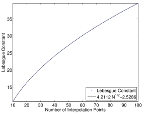
Fig. 1: Least squares approximation to the Lebesgue constant for the point set corresponding to the Gauss quadrature points augmented by $-1$ using curves of the form $a\sqrt{N}+b$

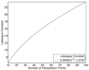
Fig. 2: Least squares approximation to the Lebesgue constant for the point set corresponding to the Radau quadrature points using curves of the form $a\sqrt{N}+b$

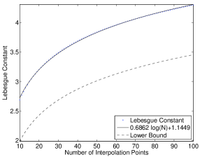
Fig. 3: Least squares approximation to the Lebesgue constant for the point set corresponding to the Radau quadrature points on $(-1,+1]$ augmented by $-1$ using curves of the form $a\log N+b$

7 Conclusions

In Gauss and Radau collocation methods for unconstrained control problems [14, 15], the error in the solution to the discrete problem is bounded by the residual for the solution to the continuous problem inserted in the discrete equations. In Section 2, we observe that the residual in the sup-norm is bounded by the distance between the derivative of the continuous solution interpolant and the derivative of the continuous solution. Proposition 1 bounds this distance in terms of the error in best approximation and the Lebesgue constant for the point set. We show that the Lebesgue constant for the point sets associated with the Gauss and Radau collocation methods is $O(\sqrt{N})$, and by the plots of Section 6, the Lebesgue constants are closely fit by curves of the form $a\sqrt{N}+b$.

References

- [1] L. Brutman, Lebesgue functions for polynomial interpolation - a survey, Annales Numer. Math., 4, pp. 111–127.
- [2] , On the Lebesgue function for polynomial interpolation, SIAM J. Numer. Anal., 15 (1978), pp. 694–704.
- [3] C. L. Darby, W. W. Hager, and A. V. Rao, Direct trajectory optimization using a variable low-order adaptive pseudospectral method, AIAA Journal of Spacecraft and Rockets, 48 (2011), pp. 433–445.
- [4] , An hp-adaptive pseudospectral method for solving optimal control problems, Optim. Control Appl. Meth., 32 (2011), pp. 476–502.
- [5] A. L. Dontchev and W. W. Hager, The Euler approximation in state constrained optimal control, Math. Comp., 70 (2001), pp. 173–203.
- [6] K. Driver, K. Jordaan, and N. Mbuyi, Interlacing of the zeros of Jacobi polynomials with different parameters, Numerical Algorithms, 49 (2008), pp. 143–152.
- [7] P. Erdős, Problems and results on the theory of interpolation, II, Acta Math. Acad. Sci. Hungar., 12 (1961), pp. 235–244.
- [8] C. C. Françolin, D. A. Benson, W. W. Hager, and A. V. Rao, Costate estimation in optimal control using integral Gaussian quadrature orthogonal collocation methods, Optim. Control Appl. Meth., DOI: 10.1002/oca.2112 (2014).
- [9] D. Garg, W. W. Hager, and A. V. Rao, Pseudospectral methods for solving infinite-horizon optimal control problems, Automatica, 47 (2011), pp. 829–837.
- [10] D. Garg, M. A. Patterson, C. L. Darby, C. Françolin, G. T. Huntington, W. W. Hager, and A. V. Rao, Direct trajectory optimization and costate estimation of finite-horizon and infinite-horizon optimal control problems using a Radau pseudospectral method, Comput. Optim. Appl., 49 (2011), pp. 335–358.
- [11] D. Garg, M. A. Patterson, W. W. Hager, A. V. Rao, D. A. Benson, and G. T. Huntington, A unified framework for the numerical solution of optimal control problems using pseudospectral methods, Automatica, 46 (2010), pp. 1843–1851.
- [12] W. W. Hager, Runge-Kutta methods in optimal control and the transformed adjoint system, Numer. Math., 87 (2000), pp. 247–282.
- [13] , Numerical analysis in optimal control, in International Series of Numerical Mathematics, K.-H. Hoffmann, I. Lasiecka, G. Leugering, J. Sprekels, and F. Tröltzsch, eds., vol. 139, Basel/Switzerland, 2001, Birkhauser Verlag, pp. 83–93.
- [14] W. W. Hager, H. Hou, and A. V. Rao, Convergence rate for a Gauss collocation method applied to unconstrained optimal control, J. Optim. Theory Appl., submitted (2015, arxiv.org/abs/1507.08263).
- [15] , Convergence rate for a Radau collocation method applied to unconstrained optimal control, SIAM Journal on Control and Optimization, submitted (2015, arxiv.org/abs/1508.03783).
- [16] N. Hale and A. Townsend, Fast and accurate computation of Gauss-Legendre and Gauss-Jacobi quadrature nodes and weights, SIAM J. Sci. Comput., 35 (2013), pp. A652–A674.
- [17] D. Jackson, The Theory of Approximation, vol. XI, Amer. Math. Soc, Colloq. Publ., Providence, RI, 1930.
- [18] V. A. Markov, Über Polynome, die in einem gegebenen Intervalle möglichst wenig von Null abweichen, Math. Ann., 77 (1916), pp. 185–191.
- [19] G. Mastroianni and G. V. Milovanović, Interpolation Processes, Basic Theory and Applications, Springer, Berlin, 2008.
- [20] M. A. Patterson, W. W. Hager, and A. V. Rao, A mesh refinement method for optimal control, Optim. Control Appl. Meth., 36 (2015), pp. 398–421.
- [21] T. J. Rivlin, An Introduction To The Approximation Of Functions, Dover Publications, New York, 1969.
- [22] G. Szegő, Orthogonal Polynomials, American Mathematical Society, Providence, RI, 1939.
- [23] L. N. Trefethen, Approximation Theory and Approximation Practice, SIAM Publications, Philadelphia, 2013.
- [24] P. Vértesi, On Lagrange interpolation, Period. Math. Hungar., 12 (1981), pp. 103–112.