Remarks on Analytic Solutions in Nonlinear Elasticity and Anti-Plane Shear Problem

Abstract

This paper revisits a well-studied anti-plane shear deformation problem formulated by Knowles in 1976 and analytical solutions in general nonlinear elasticity proposed by Gao since 1998. Based on minimum potential principle, a well-determined fully nonlinear system is obtained for isochoric deformation, which admits non-trivial states of finite anti-plane shear without ellipticity constraint. By using canonical duality theory, a complete set of analytical solutions are obtained for 3-D finite deformation problems governed by generalized neo-Hookean model. Both global and local extremal solutions to the nonconvex variational problem are identified by a triality theory. Connection between challenges in nonconvex analysis and NP-hard problems in computational science is revealed. It is proved that the ellipticity condition for general fully nonlinear boundary value problems depends not only on differential operators, but also sensitively on the external force field. The homogenous hyper-elasticity for general anti-plane shear deformation must be governed by the generalized neo-Hookean model. Knowles’ over-determined system is simply due to a pseudo-Lagrange multiplier and two extra equilibrium conditions in the plane. The constitutive condition in his theorems is naturally satisfied with $b=\lambda/2$. His ellipticity condition is neither necessary nor sufficient for general homogeneous materials to admit nontrivial states of anti-plane shear.

AMS Classification: 35Q74, 49S05, 74B20
Keywords: Nonlinear elasticity, Nonlinear PDEs, Nonconvex analysis, Ellipticity, Anti-plane shear deformation.

1 Remarks on Nonconvex Variational Problem and Challenges

Minimum total potential energy principle plays a fundamental role in continuum mechanics, especially for hyper-elasticity. One important feature is that the equilibrium equations obtained (under certain regularity conditions) by this principle are naturally compatible. Therefore, instead of the local method adopted by Knowles [15, 16], the discussion of this paper begins from the minimum potential variational problem ($({\cal P})$ for short):

$$({\cal P}):\;\;\min\left\{\Pi(\mbox{\boldmath$\chi$})=\int_{{\cal B}}{W}(\nabla\mbox{\boldmath$\chi$})d{\cal B}-\int_{S_{t}}\mbox{\boldmath$\chi$}\cdot{\bf t}dS|\;\;\mbox{\boldmath$\chi$}\in{\cal{X}}_{c}\right\},$$ (1)

where the unknown deformation $\mbox{\boldmath$\chi$}({\bf x})=\{\chi_{i}(x_{j})\}\in{\cal{X}}_{a}$ is a vector-valued mapping ${\cal B}\subset\mathbb{R}^{3}\rightarrow\omega\subset\mathbb{R}^{3}$ from a given material particle ${\bf x}=\{x_{i}\}\in{\cal B}$ in the undeformed body to a position vector in the deformed configuration $\omega$. The body is fixed on the boundary $S_{x}\subset\partial{\cal B}$, while on the remaining boundary $S_{t}=S_{x}\cap\partial{\cal B}$, the body is subjected to a given surface traction ${\bf t}({\bf x})$. In this paper, we assume

$${\cal{X}}_{a}=\{\mbox{\boldmath$\chi$}\in{\cal W}^{1,1}({\cal B};\mathbb{R}^{3})|\;\;\det(\nabla\mbox{\boldmath$\chi$})>0\;\;\mbox{\boldmath$\chi$}({\bf x})=0\;\;\forall{\bf x}\in S_{x}\},$$ (2)

where ${\cal W}^{1,1}$ is the standard notation for Sobolev space, i.e. a function space in which both $\chi$ and its weak derivative $\nabla\mbox{\boldmath$\chi$}$ have a finite $L^{1}({\cal B})$ norm. Clearly, a function in ${\cal W}^{1,1}$ is not necessarily to be smooth, or even continuous. For homogeneous hyperelastic body, the strain energy ${W}({\bf F})$ is assumed to be $C^{1}$ on its domain ${\cal{F}}_{a}\subset\mathbb{R}^{3\times 3}$, in which certain necessary constitutive constraints are included, such as

$${W}({\bf F})\geq 0\;\;\forall{\bf F}\in{\cal{F}}_{a},\;\;{W}({\bf F})\rightarrow\infty\mbox{ as }\|{\bf F}\|\rightarrow\infty.$$ (3)

For incompressible materials, the condition $\det{\bf F}=1$ should be included. Finally, ${\cal{X}}_{c}=\{\mbox{\boldmath$\chi$}\in{\cal{X}}_{a}|\;\nabla\mbox{\boldmath$\chi$}\in{\cal{F}}_{a}\}$ is the kinetically admissible space, which is nonconvex due to nonlinear constraints such as $\det(\nabla\mbox{\boldmath$\chi$})>0$. Also, the stored energy ${W}({\bf F})$ is in general nonconvex. Therefore, the nonconvex variational problem $({\cal P})$ has usually multiple local optimal solutions.

Let ${\cal{X}}_{b}\subset{\cal{X}}_{c}$ be a subspace with two additional conditions

$${\cal{X}}_{b}=\{\mbox{\boldmath$\chi$}\in{\cal{X}}_{c}|\;\;\mbox{\boldmath$\chi$}\in C^{2}({\cal B};\mathbb{R}^{3}),\;\;{W}({\bf F}(\mbox{\boldmath$\chi$}))\in C^{2}({\cal{F}}_{a};\mathbb{R})\},$$ (4)

the criticality condition $\delta\Pi(\mbox{\boldmath$\chi$};\delta\mbox{\boldmath$\chi$})=0\;\;\forall\delta\mbox{\boldmath$\chi$}\in{\cal{X}}_{b}$ leads to a nonlinear boundary-value problem

$$(BVP):\;\;\;\left\{\begin{array}[]{l}-\nabla\cdot\mbox{\boldmath$\sigma$}(\nabla\mbox{\boldmath$\chi$})=0\;\;\mbox{ in }{\cal B},\\ {\bf N}\cdot\mbox{\boldmath$\sigma$}(\nabla\mbox{\boldmath$\chi$})={\bf t}\;\;\mbox{ on }S_{t},\;\;\mbox{\boldmath$\chi$}=0\;\;\mbox{ on }S_{x}\end{array}\right.$$ (5)

where, ${\bf N}\in\mathbb{R}^{3}$ is a unit vector normal to $\partial{\cal B}$, and $\mbox{\boldmath$\sigma$}({\bf F})$ is the first Piola-Kirchhoff stress (force per unit undeformed area), defined by

$$\mbox{\boldmath$\sigma$}=\nabla{W}({\bf F}),\;\;\mbox{ or }\;\sigma_{ij}=\frac{\partial{W}({\bf F})}{\partial F_{ij}},\;\;i,j=1,2,3$$ (6)

which is also a two-point tensor.

Remark 1 (KKT Conditions, Isochoric Deformation, pseudo-Lagrange Multiplier)

Strictly speaking, there is an inequality constraint in ${\cal{X}}_{c}$, i.e. the admissible deformation condition $\det(\nabla\mbox{\boldmath$\chi$})>0$. According to the mathematical theory of non-monotone variational inequality,in addition to the equilibrium equations in $(BVP)$, we have the following KKT conditions

$$p\leq 0,\;\;\det(\nabla\mbox{\boldmath$\chi$})>0,\;\;p\det(\nabla\mbox{\boldmath$\chi$})=0$$ (7)

where $p$ is a Lagrange multiplier and $p\leq 0$ is called the condition of constraint qualification. The equality $p\det(\nabla\mbox{\boldmath$\chi$})=0$ is the well-known complementarity condition in variational inequality theory, by which we must have $p=0$ in order to guarantee the inequality constraint $\det(\nabla\mbox{\boldmath$\chi$})>0$. Therefore, this constraint is actually not active to the problem $({\cal P})$. Such an inactive constraint is not a variational constraint.

For incompressible deformation, the inequality condition $\det(\nabla\mbox{\boldmath$\chi$})>0$ in ${\cal{X}}_{c}$ should be replaced by an equality constraint $\det(\nabla\mbox{\boldmath$\chi$})=1$. In this case, $({\cal P})$ is a constrained variational problem. The KKT conditions (7) should be replaced by (see [17])

$$p\neq 0,\;\;\det{\bf F}(\mbox{\boldmath$\chi$})=1,\;\;p(\det{\bf F}(\mbox{\boldmath$\chi$})-1)=0.$$ (8)

and we must have $p({\bf x})\neq 0\mbox{ for a.e. }{\bf x}\in{\cal B}$ in order to ensure $\det{\bf F}(\mbox{\boldmath$\chi$})-1=0$. The associated $(BVP)$ should be

$$(BVP)_{p}:\;\;\left\{\begin{array}[]{l}-\nabla\cdot\mbox{\boldmath$\sigma$}(\nabla\mbox{\boldmath$\chi$},p)=0,\;\;\det(\nabla\mbox{\boldmath$\chi$})=1\;\;\mbox{ in }{\cal B},\\ {\bf N}\cdot\mbox{\boldmath$\sigma$}(\nabla\mbox{\boldmath$\chi$},p)={\bf t}\;\;\mbox{ on }S_{t},\;\;\mbox{\boldmath$\chi$}=0\;\;\mbox{ on }S_{x}.\end{array}\right.$$ (9)

in which, $\mbox{\boldmath$\sigma$}({\bf F},p)=\nabla{W}({\bf F})-p{\bf F}^{-T}$, where ${\bf F}^{-T}=({\bf F}^{T})^{-1}$. In this case, we have two variables $(\mbox{\boldmath$\chi$},p)$ and two equations in ${\cal B}$, thus, the problem $(BVP)_{p}$ is a well-defined system.

For isochoric (i.e. volume preserving) deformation, say the anti-plane shear problems, the condition $\det{\bf F}=1$ is trivially satisfied and the complementarity condition $p(\det{\bf F}-1)\equiv 0\;\;\forall p({\bf x})\neq 0\;\;a.e.$ in ${\cal B}$. In this case, the trivial condition $\det{\bf F}=1$ is not a variational constraint for $({\cal P})$ and the arbitrary parameter $p({\bf x})$ is not an unknown variable for $(BVP)_{p}$. Otherwise, the $(BVP)_{p}$ is an over-determined system. This fact in KKT theory is important for understanding Knowles’ anti-plane shear problem. Such a parameter for trivial condition can be called pseudo-Lagrange multiplier.

Physically speaking, the hydrostatic pressure $p$ is not necessary to be zero even for isochoric deformations. There are many examples in the literature, see the celebrated book by Ogden [19] as well as many famous papers by Rivlin on volume-preserving deformations of isotropic materials (simple shear, torsion, flexure, etc.). $\blacksquare$

Remark 2 (Convexity, Multi-Solutions, and NP-Hard Problems)

 
The stored energy ${W}({\bf F})$ in nonlinear elasticity is generally nonconvex. It turns out that the fully nonlinear $(BVP)$ could have multiple solutions $\{\mbox{\boldmath$\chi$}_{k}({\bf x})\}$ at each material point ${\bf x}\in{\cal B}_{s}\subset{\cal B}$. As long as the continuous domain ${\cal B}_{s}\neq\emptyset$, this solution set $\{\mbox{\boldmath$\chi$}_{k}({\bf x})\}$ can form infinitely many solutions to $(BVP)$ even ${\cal B}\subset\mathbb{R}$. It is impossible to use traditional convexity and ellipticity conditions to identify global minimizer among all these local solutions. Gao and Ogden discovered in [11] that for certain given external force field, both global and local extremum solutions are nonsmooth and can’t be obtained by Newton-type numerical methods. Therefore, Problem $({\cal P})$ is much more difficult than $(BVP)$. In computational mechanics, any direct numerical method for solving $({\cal P})$ will lead to a nonconvex minimization problem. Due to the lack of global optimality condition, it is a well-known challenging task to solve nonconvex minimization problems by traditional methods. Therefore, in computational sciences most nonconvex minimization problems are considered to be NP-hard (Non-deterministic Polynomial-time hard) [12].

Direct methods for solving nonconvex variational problems in finite elasticity have been studies extensively during the last fifty years and many generalized convexities, such as poly-, quasi- and rank-one convexities, have been proposed. For a given function $W:{\cal{F}}_{a}\rightarrow\mathbb{R}$, the following statements are well-known (see [24]):

convex $$\Rightarrow\mbox{ poly-convex }\Rightarrow\mbox{ quasi-convex }\Rightarrow\mbox{ rank-one convex}$$.

Although the generalized convexities have been well-studied for general function ${W}({\bf F})$ on matrix space $\mathbb{R}^{m\times n}$, these mathematical concepts provide only necessary conditions for local minimal solutions, and can’t be applied to general finite deformation problems. In reality, the stored energy ${W}({\bf F})$ must be nonconvex in order to model real-world phenomena, such as post-buckling and phase transitions etc. Strictly speaking, due to certain necessary constitutive constraints such as $\det{\bf F}>0$ and objectivity etc, even the domain ${\cal{F}}_{a}$ is not convex, therefore, it is not appropriate to discuss convexity of the stored energy ${W}({\bf F})$ in general nonlinear elasticity. How to identify global optimal solution has been a fundamental challenging problem in nonconvex analysis and computational science. $\blacksquare$

Remark 3 (Canonical Duality, Gap Function, and Global Extremality)

 
The objectivity is a necessary constraint for any hyper-elastic model. A real-valued function ${W}:{\cal{F}}_{a}\rightarrow\mathbb{R}$ is objective iff there exists a function $U({\bf C})$ such that $W({\bf F})=U({\bf F}^{T}{\bf F})\;\;\forall{\bf F}\in{\cal{F}}_{a}.$ By the fact that the right Cauchy-Green tensor ${\bf C}$ is an objective measure on a convex domain ${\cal{E}}_{a}=\{{\bf C}\in\mathbb{R}^{3\times 3}|\;\;{\bf C}={\bf C}^{T},\;\;{\bf C}\succ 0\}$, it is possible and natural to discuss the convexity of $U({\bf C})$. This fact lays a foundation for the canonical duality theory [6], which was developed from Gao and Strang’s original work in 1989 [13] for general nonconvex/nonsmooth variational problems in finite deformation theory. The key idea of this theory is assuming the existence of a geometrically admissible (objective) measure $\mbox{\boldmath$\xi$}=\Lambda({\bf F})$ and a canonical function $V(\mbox{\boldmath$\xi$})$ such that the following canonical transformation holds

$$\mbox{\boldmath$\xi$}=\Lambda({\bf F}):{\cal{F}}_{a}\rightarrow{\cal{E}}_{a}\;\;\Rightarrow\;\;{W}({\bf F})=V(\Lambda({\bf F})).$$ (10)

A real-valued function $V:{\cal{E}}_{a}\rightarrow\mathbb{R}$ is called canonical if the duality relation $\mbox{\boldmath$\xi$}^{*}=\nabla V(\mbox{\boldmath$\xi$}):{\cal{E}}_{a}\rightarrow{\cal{E}}^{*}_{a}$ is one-to-one and onto [6]. This canonical duality is necessary for modeling natural phenomena. Gao and Strang discovered that the directional derivative ${\Lambda}_{t}({\bf F})=\delta{\Lambda}({\bf F})$ is adjoined with the equilibrium operator, while its complementary operator ${\Lambda}_{c}({\bf F})=\Lambda({\bf F})-{\Lambda}_{t}({\bf F}){\bf F}$ leads to a so-called complementary gap function, which recovers duality gaps in traditional analysis and provides a sufficient condition for identifying both global and local extremal solutions [6, 12]. $\blacksquare$

The canonical duality theory has been applied for solving a large class of nonconvex, nonsmooth, discrete problems in multidisciplinary fields of nonlinear analysis, nonconvex mechanics, global optimization, and computational sciences, etc. A comprehensive review is given recently in [12]. The main goal of this paper is to show author’s recent analytical solutions [8] are valid for general anti-plane shear problems and can be easily generalized for solving finite deformation problems governed by generalized neo-Hookean materials. While the constitutive constraints in Knowles’ over-determined system [15] are not necessary, the hydrostatic pressure $p=p(x_{1},x_{2})$ is independent of $x_{3}$ and can’t be considered as a variational variable. Some insightful results are obtained on ellipticity condition in nonlinear analysis.

2 Complete Solutions to Generalized Neo-Hookean Material

Since the right Cauchy-Green strain ${\bf C}={\bf F}^{T}{\bf F}$ is an objective tensor, its three principal invariants

$$I_{1}({\bf C})=\mbox{tr\hskip 1.0pt}\mathbf{C},\quad I_{2}({\bf C})=\frac{1}{2}[(\mbox{tr\hskip 1.0pt}{\bf C})^{2}-\mbox{tr\hskip 1.0pt}({\bf C})^{2}],\quad I_{3}({\bf C})=\det\mathbf{C}$$ (11)

are also objective functions of ${\bf F}$. Clearly, for isochoric deformations we have $I_{3}({\bf C})=1$. The elastic body is said to be generalized neo-Hookean material if the stored energy depends only on $I_{1}$, i.e. there exists a function $V(I_{1})$ such that $W({\bf F})=V(I_{1}({\bf C}({\bf F})))$. Since $I_{1}=\mbox{tr\hskip 1.0pt}({\bf F}^{T}{\bf F})>0\;\;\forall{\bf F}\in{\cal{F}}_{a}$, the domain of $V(I_{1})$ is a convex (positive) cone ${\cal{E}}_{a}=\{x\in\mathbb{R}|\;x>0\}$, it is possible to discuss the convexity of $V(I_{1})$. Furthermore, we assume that $V(I_{1})$ is a $C^{2}({\cal{E}}_{a})$ canonical function. Then the canonical transformation (10) for the generalized neo-Hookean model is

$$\xi={\Lambda}({\bf F})=\mbox{tr\hskip 1.0pt}({\bf F}^{T}{\bf F}):{\cal{F}}_{a}\rightarrow{\cal{E}}_{a},\;\;{W}({\bf F})=V(\xi({\bf F})).$$ (12)

For a given external force ${\bf t}({\bf x})$ on ${S_{t}}$, we introduce a statically admissible space

$${{\cal{T}}}_{a}=\{{{\bf T}}\in{\cal C}^{1}[{\cal B};\mathbb{R}^{3\times 3}]\;|\;\;\nabla\cdot{\bf T}=0\;\;\mbox{ in }{\cal B},\;\;{\bf N}\cdot{\bf T}={\bf t}\mbox{ on }S_{t}\}.$$ (13)

Thus for any given ${\bf T}\in{\cal{T}}_{a}$, the primal problem $({\cal P})$ for the generalized neo-Hookean material can be written in following canonical form

$$({\cal P})_{g}:\;\;\min\left\{\Pi(\mbox{\boldmath$\chi$})=\int_{{\cal B}}P(\nabla\mbox{\boldmath$\chi$}){\rm d}{\cal B},\;\;|\;\;\forall\mbox{\boldmath$\chi$}\in{\cal{X}}_{c}\right\},$$ (14)

where ${\cal{X}}_{c}=\{\mbox{\boldmath$\chi$}\in{\cal{X}}_{a}|\;\Lambda(\nabla\mbox{\boldmath$\chi$})\in{\cal{E}}_{a}\}$ and the integrand $P:{\cal{F}}_{a}\rightarrow\mathbb{R}$ is defined by

$$P({\bf F})=V(\Lambda({\bf F}))-\mbox{tr\hskip 1.0pt}({\bf F}{\bf T}).$$ (15)

The criticality condition for this canonical variational problem leads to the following canonical boundary value problem

$$(BVP)_{g}:\;\;\nabla\cdot[2\zeta(\nabla\mbox{\boldmath$\chi$})]=0\;\;\mbox{ in }{\cal B},\;\;{\bf N}\cdot[2\zeta(\nabla\mbox{\boldmath$\chi$})]={\bf t}\;\mbox{ on }{S_{t}},\;\;\mbox{\boldmath$\chi$}=0\;\;\mbox{ on }S_{x}$$ (16)

which are identical to $(BVP)$ since $\nabla{W}({\bf F})=2{\bf F}[\nabla V(\xi)]=2\zeta{\bf F}$. To solve this fully nonlinear boundary value problem is very difficult for direct methods, but easy for the canonical duality theory.

By the canonical assumption of $V(\xi)$, the duality relation $\zeta=\nabla V(\xi):{\cal{E}}_{a}\rightarrow{\cal{E}}^{*}_{a}$ is invertible. The complementary energy can be defined uniquely by the Legendre transformation

$$V^{*}(\zeta)=\{\xi\zeta-V(\xi)|\;\zeta=\nabla V(\xi)\}.$$ (17)

Clearly, the function $V:{\cal{E}}_{a}\rightarrow\mathbb{R}$ is canonical if and only if the following canonical duality relations hold on ${\cal{E}}_{a}\times{\cal{E}}^{*}_{a}$

$$\zeta=\nabla V(\xi)\;\;\Leftrightarrow\;\;\xi=\nabla V^{*}(\zeta)\;\;\Leftrightarrow\;\;V(\xi)+V^{*}(\zeta)=\xi\zeta.$$ (18)

Using $V(\xi)=\xi\zeta-V^{*}(\zeta)$, the nonconvex function $P({\bf F})$ can be written as the so-called total complementary function on ${\cal{X}}_{a}\times{\cal{E}}^{*}_{a}$

$$\Xi({\bf F},\zeta)={\Lambda}({\bf F})\zeta-V^{*}(\zeta)-\mbox{tr\hskip 1.0pt}({\bf T}{\bf F}).$$ (19)

The canonical dual function can be obtained by the canonical dual transformation:

$$P^{d}(\zeta)=\{\Xi({\bf F},\zeta)|\;\;\nabla_{{\bf F}}\Xi({\bf F},\zeta)=0\}=-V^{*}(\zeta)-\frac{1}{4}\zeta^{-1}\tau^{2},\;\;\;\tau^{2}=\mbox{tr\hskip 1.0pt}({\bf T}^{T}{\bf T}).$$ (20)

Thus, the pure complementary energy principle, first proposed in 1998 [4], leads to the following canonical dual variational problem

$$({\cal P}^{d})_{g}:\;\;\;\;{\rm sta}\left\{\Pi^{d}(\zeta)=\int_{{\cal B}}P^{d}(\zeta){\rm d}{\cal B}\;|\;\;\zeta\in{\cal{S}}_{a}\right\},$$ (21)

where ${\rm sta}\{\Pi^{d}(\zeta)|\;\zeta\in{\cal{S}}_{a}\}$ stands for finding stationary point of $\Pi^{d}(\zeta)$ on the canonical dual feasible space ${\cal{S}}_{a}=\{\zeta\in{\cal{E}}^{*}_{a}|\;\zeta^{-1}\tau^{2}\in L^{1}({\cal B})\}$.

Since the canonical dual variable $\zeta$ is a scalar-valued function, the criticality condition $\delta\Pi^{d}(\zeta)=0$ leads to a so-called canonical dual algebraic equation (see [6]):

$$4\zeta^{2}\nabla V^{*}(\zeta)=\tau^{2}$$ (22)

Note that $\nabla V^{*}(\zeta):{\cal{E}}^{*}_{a}\rightarrow{\cal{E}}_{a}$ is also one-to-one and onto, this equation has at least one solution for any given $\tau^{2}=\mbox{tr\hskip 1.0pt}({\bf T}^{T}{\bf T})\geq 0$ and $\zeta=0$ only if $\tau=0$. Therefore, $P^{d}(\zeta)$ is well-defined. Due to the nonlinearity, the solution may not be unique [8]. By the pure complementary energy principle proposed by Gao in 1999 (see [6]), we have

Theorem 1 (Pure Complementary Energy Principle)

For any given nontrivial ${\bf t}\neq 0$ such that ${\bf T}\in{\cal{T}}_{a}$, (22) has at least one solution $\zeta_{k}\neq 0$, the deformation vector defined by

$$\mbox{\boldmath$\chi$}_{k}({\bf x})=\frac{1}{2}\int_{{\bf x}_{0}}^{\bf x}\zeta_{k}^{-1}{\bf T}\cdot\mbox{d}{\bf x}$$ (23)

along any path from ${\bf x}_{0}\in S_{x}$ to ${\bf x}\in{\cal B}$ is a critical point of $\Pi(\mbox{\boldmath$\chi$})$ and $\Pi(\mbox{\boldmath$\chi$}_{k})=\Pi^{d}(\zeta_{k})$.

This principle shows that by the canonical dual transformation, the nonlinear partial differential equation in $(BVP)$ for generalized neo-Hookean model can be converted to an algebraic equation (22), which can be solved to obtain a complete set of solutions (see [8, 9]).

Since ${\cal{S}}_{a}$ is nonconvex, in order to identify global and local optimal solutions, we need the following convex subsets

$${\cal{S}}_{a}^{+}=\{\zeta\in{\cal{S}}_{a}|\;\zeta>0\},\;\;\;\bar{\cal{S}}_{a}^{+}=\{\zeta\in{\cal{S}}_{a}|\;\zeta\geq 0\},\;\;{\cal{S}}_{a}^{-}=\{\zeta\in{\cal{S}}_{a}|\;\zeta<0\}.$$ (24)

Then by the canonical duality-triality theory developed in [6] we have the following theorem.

Theorem 2

Suppose that $V:{\cal{E}}_{a}\rightarrow\mathbb{R}$ is convex and for a given ${\bf T}\in{\cal{T}}_{a}$ such that $\{\zeta_{k}\}$ is a solution set to (22), ${\bf F}_{k}=\frac{1}{2}\zeta^{-1}_{k}{\bf T}$, and $\mbox{\boldmath$\chi$}_{k}$ is defined by (23), we have the following statements.

1. If $\zeta_{k}\in\bar{\cal{S}}_{a}^{+}$, then $\nabla^{2}{W}({\bf F}_{k})\succeq 0$ and $\mbox{\boldmath$\chi$}_{k}$ is a global minimal solution to $({\cal P})_{g}$.

2. If $\zeta_{k}\in{\cal{S}}_{a}^{-}$ and $\nabla^{2}{W}({\bf F}_{k})\succ 0$, then $\mbox{\boldmath$\chi$}_{k}$ is a local minimal solution to $({\cal P})_{g}$.

3. If $\zeta_{k}\in{\cal{S}}_{a}^{-}$ and $\nabla^{2}{W}({\bf F}_{k})\prec 0$, then $\mbox{\boldmath$\chi$}_{k}$ is a local maximal solution to $({\cal P})_{g}$.

If $\{\zeta_{k}\}\subset\bar{\cal{S}}^{+}_{a}$, then $\{\mbox{\boldmath$\chi$}_{k}\}$ is a convex set. The problem $({\cal P})_{g}$ has a unique solution if $\{\zeta_{k}\}\subset{\cal{S}}^{+}_{a}$.

Proof. By using chain rule for ${W}({\bf F})=V(\xi({\bf F}))$ we have $\nabla{W}({\bf F})=2{\bf F}[\nabla V(\xi)]=2\zeta{\bf F}$, and

$$\nabla^{2}{W}({\bf F})=2\zeta{\bf I}\otimes{\bf I}+4h(\xi){\bf F}\otimes{\bf F},$$ (25)

where $\mathbf{I}$ is an identity tensor in $\mathbb{R}^{3\times 3}$, $h(\xi)=\nabla^{2}V(\xi)\geq 0$ due to the convexity of $V$ on ${{\cal{E}}_{a}}$. Therefore, $\nabla^{2}{W}({\bf F}_{k})\succeq 0$ if $\zeta_{k}\in\bar{\cal{S}}^{+}_{a}$.

To prove $\mbox{\boldmath$\chi$}_{k}$ is a global minimizer of $({\cal P})$, we follow Gao and Strang’s work in 1989 [13]. By the convexity of $V(\xi)$ on its convex domain ${\cal{E}}_{a}$, we have

$$V(\xi)-V(\xi_{k})\geq(\xi-\xi_{k})\zeta_{k}\;\;\;\;\forall\xi,\;\xi_{k}\in{\cal{E}}_{a},\;\;\zeta_{k}=\nabla V(\xi_{k}).$$ (26)

For any given variation $\delta\mbox{\boldmath$\chi$}$, we let $\mbox{\boldmath$\chi$}=\mbox{\boldmath$\chi$}_{k}+\delta\mbox{\boldmath$\chi$}$. Then we have [13]

$$\Lambda(\nabla\mbox{\boldmath$\chi$})=\mbox{tr\hskip 1.0pt}[(\nabla\mbox{\boldmath$\chi$})^{T}(\nabla\mbox{\boldmath$\chi$})]=\Lambda(\nabla\mbox{\boldmath$\chi$}_{k})+{\Lambda}_{t}(\nabla\mbox{\boldmath$\chi$}_{k})(\nabla\delta\mbox{\boldmath$\chi$})-\Lambda_{c}(\nabla\delta\mbox{\boldmath$\chi$}),$$ (27)

where ${\Lambda}_{t}({\bf F})\delta{\bf F}=2\mbox{tr\hskip 1.0pt}[{\bf F}^{T}(\delta{\bf F})]$ and $\Lambda_{c}(\delta\mbox{\boldmath$\chi$})=-\Lambda(\delta\mbox{\boldmath$\chi$})$. Clearly, ${\Lambda}({\bf F})={\Lambda}_{t}({\bf F}){\bf F}+{\Lambda}_{c}({\bf F})$. Then combining the inequality (26) and (27), we have

$$\Pi(\mbox{\boldmath$\chi$})-\Pi(\mbox{\boldmath$\chi$}_{k}) \geq \int_{\cal B}2\zeta_{k}\mbox{tr\hskip 1.0pt}[(\nabla\mbox{\boldmath$\chi$}_{k})^{T}(\nabla\delta\mbox{\boldmath$\chi$})]{\rm d}{\cal B}-\int_{S_{t}}\delta\mbox{\boldmath$\chi$}\cdot{\bf t}{\rm d}S+\int_{\cal B}\zeta_{k}\mbox{tr\hskip 1.0pt}[(\nabla\mbox{\boldmath$\chi$})^{T}(\nabla\mbox{\boldmath$\chi$})]{\rm d}{\cal B}$$ (28)

$$= \int_{\cal B}[2\zeta_{k}(\nabla\mbox{\boldmath$\chi$}_{k})-{\bf T}]:(\nabla\delta\mbox{\boldmath$\chi$}){\rm d}{\cal B}+G_{ap}(\delta\mbox{\boldmath$\chi$},\zeta_{k})\;\;\forall\mbox{\boldmath$\chi$},\;\delta\mbox{\boldmath$\chi$}\in{\cal{X}}_{c}$$

for any given ${\bf T}\in{\cal{T}}_{a}$, where

$$G_{ap}(\mbox{\boldmath$\chi$},\zeta)=\int_{\cal B}-\Lambda_{c}(\nabla\mbox{\boldmath$\chi$})\zeta{\rm d}{\cal B}=\int_{\cal B}\zeta\mbox{tr\hskip 1.0pt}[(\nabla\mbox{\boldmath$\chi$})^{T}(\nabla\mbox{\boldmath$\chi$})]{\rm d}{\cal B}$$ (29)

is the complementary gap function introduced in [13]. If $\mbox{\boldmath$\chi$}_{k}$ is a critical point of $\Pi(\mbox{\boldmath$\chi$})$, then we have

$$\int_{\cal B}[2(\nabla\mbox{\boldmath$\chi$}_{k})\zeta_{k}-{\bf T}]:(\nabla\delta\mbox{\boldmath$\chi$}){\rm d}{\cal B}=0\;\;\forall\delta\mbox{\boldmath$\chi$}\in{\cal{X}}_{c},\;\;\forall{\bf T}\in{\cal{T}}_{a}$$

Thus, we have $\Pi(\mbox{\boldmath$\chi$})-\Pi(\mbox{\boldmath$\chi$}_{k})\geq G_{ap}(\delta\mbox{\boldmath$\chi$},\zeta_{k})\geq 0\;\;\forall\delta\mbox{\boldmath$\chi$}\in{\cal{X}}_{c}\;\mbox{ if }\zeta_{k}\in\bar{\cal{S}}_{a}^{+}.$ This shows that $\mbox{\boldmath$\chi$}_{k}$ is a global minimizer of $({\cal P})_{g}$.

To prove the local extremality, we replace ${\bf F}_{k}$ in (25) by ${\bf F}_{k}=\frac{1}{2}\zeta^{-1}_{k}{\bf T}$ such that

$${\bf G}(\zeta_{k})=\nabla^{2}{W}({\bf F}_{k})=2\zeta_{k}{\bf I}\otimes{\bf I}+\zeta_{k}^{-2}h(\xi_{k}){\bf T}\otimes{\bf T},$$ (30)

where $\xi_{k}=\nabla V^{*}(\zeta_{k})$. Clearly, for a given ${\bf T}\in{\cal{T}}_{a}$ such that $\zeta_{k}\in{\cal{S}}^{-}_{a}$, the Hessian $\nabla^{2}{W}({\bf F}_{k})$ could be either positive or negative definite. The total potential $\Pi(\mbox{\boldmath$\chi$}_{k})$ is locally convex if the Legendre condition $\nabla^{2}{W}(\nabla\mbox{\boldmath$\chi$}_{k})\succeq 0$ holds, locally concave if $\nabla^{2}{W}(\nabla\mbox{\boldmath$\chi$}_{k})\prec 0$. Since $\mbox{\boldmath$\chi$}_{k}$ is a global minimizer when $\zeta_{k}\in\bar{\cal{S}}^{+}_{a}$, therefore, for $\zeta_{k}\in{\cal{S}}^{-}_{a}$, the stationary solution $\mbox{\boldmath$\chi$}_{k}$ is a local minimizer if $\nabla^{2}{W}(\nabla\mbox{\boldmath$\chi$}_{k})\succeq 0$ and, by the triality theory[6, 12], $\mbox{\boldmath$\chi$}_{k}$ is a biggest local maximizer if $\nabla^{2}{W}(\nabla\mbox{\boldmath$\chi$}_{k})\prec 0$.

If $\{\zeta_{k}\}\subset\bar{\cal{S}}^{+}_{a}$, then all the solutions $\{\mbox{\boldmath$\chi$}_{k}\}$ are global minimizers and form a convex set. Since $P^{d}(\zeta)$ is strictly concave on the open convex set ${\cal{S}}^{+}_{a}$, the condition $\{\zeta_{k}\}\subset{\cal{S}}^{+}_{a}$ implies the unique solution of (22). In this case, both problems $({\cal P})$ and $(BVP)$ have at most one solution. $\Box$

Theorem 3 (Triality Theory)

For any given ${\bf T}\in{\cal{T}}_{a}$, let $\zeta_{k}$ be a critical point of $({\cal P}^{d})_{g}$, the vector $\mbox{\boldmath$\chi$}_{k}$ be defined by (23), and ${\cal{X}}_{o}\times{\cal{S}}_{o}\subset{\cal{X}}_{c}\times{\cal{S}}^{-}_{o}$ a neighborhood of $(\mbox{\boldmath$\chi$}_{k},\zeta_{k})$.

If $\zeta_{k}\in{\cal{S}}^{+}_{a}$, then

$$\Pi(\mbox{\boldmath$\chi$}_{k})=\min_{\mbox{\boldmath$\chi$}\in{\cal{X}}_{c}}\Pi(\mbox{\boldmath$\xi$})=\max_{\zeta\in{\cal{S}}^{+}_{a}}\Pi^{d}(\zeta)=\Pi^{d}(\zeta_{k}).$$ (31)

If $\zeta_{k}\in{\cal{S}}^{-}_{a}$ and ${\bf G}(\zeta_{k})\succ 0$, then

$$\Pi(\mbox{\boldmath$\chi$}_{k})=\min_{\mbox{\boldmath$\chi$}\in{\cal{X}}_{o}}\Pi(\mbox{\boldmath$\xi$})=\min_{\zeta\in{\cal{S}}_{o}}\Pi^{d}(\zeta)=\Pi^{d}(\zeta_{k}).$$ (32)

If $\zeta_{k}\in{\cal{S}}^{-}_{a}$ and ${\bf G}(\zeta_{k})\prec 0$, then

$$\Pi(\mbox{\boldmath$\chi$}_{k})=\max_{\mbox{\boldmath$\chi$}\in{\cal{X}}_{o}}\Pi(\mbox{\boldmath$\xi$})=\max_{\zeta\in{\cal{S}}_{o}}\Pi^{d}(\zeta)=\Pi^{d}(\zeta_{k}).$$ (33)

This theorem shows that the triality theory can be used to identify both global and local extremum solutions to the variational problem $({\cal P})_{g}$ and the nonconvex minimum variational problem $({\cal P})_{g}$ is canonically equivalent to the following concave maximization problem over an open convex set ${\cal{S}}^{+}_{a}$, i.e.

$$({\cal P}^{\sharp})_{g}:\;\;\;\;\max\left\{\Pi^{d}(\zeta)=\int_{{\cal B}}P^{d}(\zeta){\rm d}{\cal B}\;|\;\;\zeta\in{\cal{S}}^{+}_{a}\right\},$$ (34)

which is much easier to solve for obtaining global optimal solution of $({\cal P})_{g}$.

3 Generalized Quasiconvexity, G-Ellipticity, and Uniqueness

The ellipticity is a classical concept originally from linear partial differential systems, where the deformation is a scalar-valued function $\chi:{\cal B}\rightarrow\mathbb{R}$ and stored energy is a quadratic function ${W}(\mbox{\boldmath$\gamma$})=\frac{1}{2}\mbox{\boldmath$\gamma$}^{T}{{\bf H}}\mbox{\boldmath$\gamma$}$ of $\mbox{\boldmath$\gamma$}=\nabla\chi\in\mathbb{R}^{3}$. The linear operator

$$L[\chi]=-\nabla\cdot[{\bf H}(\nabla\chi)]=-[h_{ij}\chi_{,j}]_{,i}$$

is called elliptic if ${\bf H}=\{h_{ij}\}$ is positive definite. In this case, the function $P(\mbox{\boldmath$\gamma$})={W}(\mbox{\boldmath$\gamma$})-\mbox{\boldmath$\gamma$}^{T}{\mbox{\boldmath$\tau$}}$ is convex and its level set is an ellipse for any given ${\mbox{\boldmath$\tau$}}\in\mathbb{R}^{3}$. This concept has been extended to nonlinear analysis. The fully nonlinear partial differential equation in $(BVP)$ (5) is called elliptic if the stored energy ${W}({\bf F})$ is rank-one convex. In the case $W\in{C}^{2}$, the rank-one convexity is equivalent to the Legendre-Hadamard (LH) condition:

$$({\bf a}\otimes{\bf a}):\nabla^{2}{W}({\bf F}):({\mbox{\boldmath$\eta$}}\otimes{\mbox{\boldmath$\eta$}})\geq 0\;\;\forall{\bf a},\mbox{\boldmath$\eta$}\in\mathbb{R}^{3},\;\;\forall{\bf F}\in{\cal{F}}_{a}\subset\mathbb{R}^{m\times n}.$$ (35)

The $(BVP)$ is called strong elliptic if the inequality holds strictly. In this case, $(BVP)$ has at most one solution. In vector space, the LH condition is equivalent to Legendre condition $\nabla^{2}{W}(\mbox{\boldmath$\gamma$})\succeq 0\;\;\forall\mbox{\boldmath$\gamma$}\in\mathbb{R}^{n}$.

Clearly, the LH condition is only a sufficient condition for local minimizer of the variational problem $({\cal P})$. In order to identify ellipticity, one must to check LH condition for all local solutions, which is impossible for general fully nonlinear problems. Also, the traditional ellipticity definition depends only on the stored energy ${W}({\bf F})$ regardless of the linear term in $P({\bf F})$. This definition works only for convex systems since the linear term can’t change the convexity of $P({\bf F})$. But this is not true for nonconvex systems. To see this, let us consider the St. Venant-Kirchhoff material

$$W({\bf F})=\frac{1}{2}{\bf E}:{\bf H}:{\bf E},\;\;{\bf E}=\frac{1}{2}[({\bf F})^{T}({\bf F})-{\bf I}],$$ (36)

where ${\bf I}$ is a unit tensor in $\mathbb{R}^{3\times 3}$. Clearly, this function is not even rank-one convex. A special case of this model is the well-known double-well potential ${W}(\mbox{\boldmath$\gamma$})=\frac{1}{2}(\frac{1}{2}|\mbox{\boldmath$\gamma$}|^{2}-1)^{2}$. In this case, if we let $\xi=\Lambda(\mbox{\boldmath$\gamma$})=\frac{1}{2}|\mbox{\boldmath$\gamma$}|^{2}-1$ be an objective measure, we have the canonical function $V(\xi)=\frac{1}{2}\xi^{2}$. In this case, the canonical dual algebraic equation (22) is a cubic equation (see [6]) $2\zeta^{2}(\zeta+1)=\tau^{2}$, which has at most three real solutions $\{\zeta_{k}({\bf x})\}$ at each ${\bf x}\in{\cal B}$ satisfying $\zeta_{1}\geq 0\geq\zeta_{2}\geq\zeta_{3}$. It was proved in [6] (Theorem 3.4.4, page 133) that for a given force ${\bf t}({\bf x})$, if $\tau^{2}({\bf x})>8/27\;\;\forall{\bf x}\in{\cal B}\subset\mathbb{R}$, then $(BVP)_{g}$ has only one solution on ${\cal B}$. If $\tau^{2}({\bf x})<8/27\;\;\forall{\bf x}\in{\cal B}_{s}\subset{\cal B}$, then $(BVP)_{g}$ has three solutions $\{\chi_{k}({\bf x})\}$ at each ${\bf x}\in{\cal B}_{s}$, i.e. $\Pi(\chi)$ is nonconvex on ${\cal B}_{s}$. It was shown by Gao and Ogden that these solutions are nonsmooth if $\tau({\bf x})$ changes its sign on ${\cal B}_{s}$ [11].

Analytical solutions for general 3-D finite deformation problem $({\cal P})$ were first proposed by Gao in 1998-1999 [4, 5]. It is proved recently [9] that for St Venant-Kirchhoff material, the problem $({\cal P})$ could have 24 critical solutions at each material point ${\bf x}\in{\cal B}$, but only one global minimizer. The solution is unique if the external force is sufficiently bigger.

The geometrical explanation for ellipticity and Theorem 2 is illustrated by Fig. 1, which shows that the nonconvex function $P(\mbox{\boldmath$\gamma$})=\frac{1}{2}(\frac{1}{2}|\mbox{\boldmath$\gamma$}|^{2}-1)^{2}-\mbox{\boldmath$\gamma$}^{T}{\mbox{\boldmath$\tau$}}$ depends sensitively on the external force ${\mbox{\boldmath$\tau$}}\in\mathbb{R}^{2}$. If $|{\mbox{\boldmath$\tau$}}|$ is bigger enough, $P(\mbox{\boldmath$\gamma$})$ has only one minimizer and its level set is an ellipse (Fig. 1 (b)). Otherwise, $P(\mbox{\boldmath$\gamma$})$ has multiple local minimizers and its level set is not an ellipse. For ${\mbox{\boldmath$\tau$}}=0$, it is well-known Mexican-hat in theoretical physics (Fig. 1 (a)).

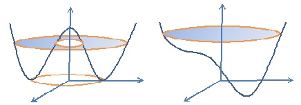
Figure 1: Graphs and level sets of $P({\bf x})$ with ${{\mbox{\boldmath$\tau$}}}=0$ (left) and ${{\mbox{\boldmath$\tau$}}}\neq 0$ (right)

Fig. 1 shows that although $P(\mbox{\boldmath$\gamma$})$ has only one global minimizer for certain given $\tau$, the function is still nonconvex. Such a function is called quasiconvex in the context of global optimization. In order to distinguish this type of functions with Morry’s quasiconvexity in nonconvex analysis, a generalized definition on a tensor space ${\cal{F}}_{a}\subset\mathbb{R}^{m\times n}$ could be convenient.

Definition 1 (G-Quasiconvexity)

A function $P:{\cal{F}}_{a}\subset\mathbb{R}^{m\times n}\rightarrow\mathbb{R}$ is called G-quasiconvex if its domain ${\cal{F}}_{a}$ is convex and

$$P(\theta{\bf F}+(1-\theta){\bf T})\leq\max\{P({\bf F}),P({\bf T})\}\;\;\forall{\bf F},\;{\bf T}\in{\cal{F}}_{a},\;\;\forall\theta\in[0,1].$$ (37)

It is called strictly G-quasiconvex if the inequality holds strictly.

For a given function $P:{\cal{F}}_{a}\rightarrow\mathbb{R}$, its level set and sub-level set of height $\alpha\in\mathbb{R}$ are defined, respectively, as the following

$${\cal L}_{\alpha}(P)=\{{\bf F}\in{\cal{F}}_{a}\;|\;\;P({\bf F})=\alpha\},\;\;{\cal L}^{\flat}_{\alpha}(P)=\{{\bf F}\in{\cal{F}}_{a}\;|\;\;P({\bf F})\leq\alpha\},\;\;\alpha\in\mathbb{R}.$$ (38)

Moreover, we may need a generalize ellipticity definition for nonconvex systems.

Definition 2 (G-Ellipticity)

For a given function $P:{\cal{F}}_{a}\rightarrow\mathbb{R}$ and $\alpha\in\mathbb{R}$, its level set ${\cal L}_{\alpha}(P)$ is said to be a G-ellipse if it is a closed, simply connected set. For a given ${\bf t}$ such that ${\bf T}\in{\cal{T}}_{a}$, the $(BVP)$ is said to be $G$-elliptic if the total potential function $P({\bf F})$ is G-quasiconvex on ${\cal{F}}_{a}$. $(BVP)$ is strongly elliptic if $P({\bf F})$ is strictly G-quasiconvex.

Clearly, we have the following statements:

$$P({\bf F}) \Leftrightarrow {\cal L}^{\flat}_{\alpha}(P) \Leftrightarrow {\cal L}_{\alpha}(P) \forall\alpha\in\mathbb{R}$$ is G-quasiconvex is convex is G-ellipse . (39)

$$\mbox{ $P({\bf F})$ convex $\Rightarrow$ rank-one convex $\Rightarrow$ G-quasiconvex $\Rightarrow$ $(BVP)$ is G-elliptic}.$$ (40)

This statement shows a fact in nonconvex systems, i.e. the number of solutions to a nonlinear equation depends not only on the stored energy, but also (mainly) on the external force field. The nonlinear partial differential equation in $(BVP)$ is elliptic only if it is G-elliptic. $(BVP)$ has at most one solution if the integrand $P({\bf F})$ in the total potential $\Pi(\mbox{\boldmath$\chi$})$ is strictly G-quasiconvex on ${\cal{F}}_{a}$.

In global optimization, the most simple quadratic integer programming problem

$$({\cal P})_{i}:\;\;\;\min\left\{\Pi({\bf x})=\frac{1}{2}{\bf x}^{T}{\bf Q}{\bf x}-{\bf x}^{T}{\bf t}\;\;|\;\;{\bf x}\in\{0,1\}^{n}\subset\mathbb{R}^{n}\right\}$$

could have up to $2^{n}$ local minimizers due to the indefinite matrix ${\bf Q}$ and the integer constraint. Such a nonconvex discrete optimization problem is considered as NP-hard in computer science. However, by using canonical transformation $\mbox{\boldmath$\xi$}=\{x_{i}(x_{i}-1)\}$, the canonical dual of this discrete problem is a concave maximization over a convex set in continuous space. It was proved in [7] that as long as the source term ${\bf t}=\{t_{i}\}$ is bigger enough, ${\cal{S}}^{+}_{a}\neq\emptyset$ and $({\cal P})_{i}$ is not NP-hard. The decision variable is simply $\{x_{i}\}=\{0\mbox{ if }t_{i}<0,\;1\;\mbox{ if }t_{i}>0\}$ (Theorem 8, [7]).

4 Anti-plane Shear Deformation Problems

Now let us consider a special case that the homogeneous elastic body ${\cal B}\subset\mathbb{R}^{3}$ is a cylinder with generators parallel to the ${\bf e}_{3}$ axis and with cross section a sufficiently nice region $\Omega\subset\mathbb{R}^{2}$ in the ${\bf e}_{1}\times{\bf e}_{2}$ plane. The so-called anti-plane shear deformation is defined by (see Knowles 1976, [15])

$$\mbox{\boldmath$\chi$}({\bf x})=\left\{\lambda^{-\frac{1}{2}}x_{1},\;\;\lambda^{-\frac{1}{2}}x_{2},\;\;\lambda x_{3}+{u}({x}_{1},{x}_{2})\right\}:\Omega\rightarrow\mathbb{R}^{3},$$ (41)

where $({x}_{1},{x}_{2},{x}_{3})$ are cylindrical coordinates in the reference configuration ${\cal B}$ relative to a cylindrical basis $\{{\bf e}_{i}\},\;i=1,2,3$, the parameter $\lambda$ is a positive constant, and ${u}:\Omega\rightarrow\mathbb{R}$ is the amount of shear (locally a simple shear) in the planes normal to ${\bf e}_{3}$. On ${\Gamma_{\chi}}\subset\partial\Omega$, the homogenous boundary condition is given ${u}(x_{\alpha})=0\;\;\forall x_{\alpha}\in{\Gamma_{\chi}},\;\;\alpha=1,2.$ On the remaining boundary ${\Gamma_{t}}=\partial\Omega\cap{\Gamma_{\chi}}$, the cylinder is subjected to the shear force

$${\bf t}({\bf x})=t({\bf x}){\bf e}_{3}\;\;\forall{\bf x}\in{\Gamma_{t}},$$

where $t:{\Gamma_{t}}\rightarrow\mathbb{R}$ is a prescribed function. According to Knowles, the deformation (41) may be thought of as one in which the body first undergoes an axial elongation (or contraction) of stretch ratio $\lambda$ (regarded as given), and is then subjected to an anti-plane shear with out-of-plane displacement ${u}$. For this anti-plane shear deformation we have

$$\mathbf{F}=\nabla\mbox{\boldmath$\chi$}=\left(\begin{array}[]{ccc}\lambda^{-\frac{1}{2}}&0&0\\ 0&\lambda^{-\frac{1}{2}}&0\\ {u}_{,1}&{u}_{,2}&\lambda\end{array}\right),\;\;\;\;\mathbf{C}=\mathbf{F}^{\rm T}{\bf F}=\left(\begin{array}[]{ccc}\lambda^{-1}+{u}_{,1}^{2}&{u}_{,1}{u}_{,2}&\lambda{u}_{,1}\\ {u}_{,1}{u}_{,2}&\lambda^{-1}+{u}_{,2}^{2}&\lambda{u}_{,2}\\ \lambda{u}_{,1}&\lambda{u}_{,2}&\lambda^{2}\end{array}\right),$$ (42)

where ${u}_{,\alpha}$ represents $\partial{u}/\partial x_{\alpha}$ for $\alpha=1,2$. By the notation $|\nabla{u}|^{2}={u}_{,1}^{2}+{u}_{,2}^{2}$, we have

$$I_{1}({\bf C})=\lambda_{1}+|\nabla{u}|^{2},\;\;I_{2}({\bf C})=\lambda_{2}+\lambda^{-1}|\nabla{u}|^{2},\;\;I_{3}({\bf C})\equiv 1,$$ (43)

where $\lambda_{1}=\lambda^{2}+2\lambda^{-1},\;\lambda_{2}=\lambda^{-2}+2\lambda$. Particularly,

$$I_{1}({\bf C})=I_{2}({\bf C})=3+|\nabla{u}|^{2}\;\;\mbox{ if }\lambda=1.$$ (44)

Lemma 1

For any given $\lambda>0$, the homogenous hyper-elasticity for general anti-plane shear deformation must be governed by a generalized neo-Hookean model, i.e. ${W}({\bf F})=V(I_{1})$. Particularly, the Mooney-Rivlin model is identical to the neo-Hookean model subjected to a constant, i.e. ${W}({\bf F})=A(I_{1}-3)+B$ with $B=0$ if $\lambda=1$.

The proof is elementary, i.e. by the fact that $I_{2}=\lambda^{-1}I_{1}+a$, $a=\lambda_{2}-\lambda^{-1}\lambda_{1}$, we have

$${W}({\bf F})=\bar{W}(I_{1},I_{2})=\bar{W}(I_{1},\lambda^{-1}I_{1}+a)=V(I_{1}),\;\;\forall\lambda>0.$$

Moreover, let $A=c_{1}+c_{2}\lambda^{-1},\;\;B=c_{2}(3\lambda^{-1}-3+\lambda_{2}-\lambda_{1}\lambda^{-1})$, we have the Mooney-Rivlin model ${W}({\bf F})=c_{1}(I_{1}-3)+c_{2}(I_{2}-3)=A(I_{1}-3)+B$.

The fact $\det{\bf F}\equiv 1$ shows that the anti-plane shear state (41) is an isochoric deformation. Therefore, the kinetically admissible displacement space ${\cal{X}}_{c}$ can be simply replaced by a convex set

$${\cal{U}}_{c}=\{{u}(x_{1},x_{2})\in{\cal W}^{1,1}(\Omega;\mathbb{R})|\;\;{u}(x_{\alpha})=0\;\;\forall x_{\alpha}\in{\Gamma_{\chi}}\}.$$ (45)

Thus, in terms of $\mbox{\boldmath$\gamma$}=\nabla{u}$, $\xi=\Lambda(\mbox{\boldmath$\gamma$})=|\mbox{\boldmath$\gamma$}|^{2}+\lambda_{1}$, and ${W}({\bf F}(\mbox{\boldmath$\gamma$}))=V(\Lambda(\mbox{\boldmath$\gamma$}))$, for any given

$${\mbox{\boldmath$\tau$}}\in{\cal{T}}_{a}=\{{\mbox{\boldmath$\tau$}}\in C^{1}[\Omega;\mathbb{R}^{2}]|\;\;\nabla\cdot{\mbox{\boldmath$\tau$}}=0\;\;\mbox{ in }\Omega,\;\;{\bf n}\cdot{\mbox{\boldmath$\tau$}}=t\;\;\mbox{ on }{\Gamma_{t}}\}$$

Problem $({\cal P})_{g}$ for the general anti-plane shear deformation problem has the following form

$$({\cal P})_{s}:\;\;\min\left\{\Pi({u})=\int_{\Omega}P(\nabla{u}){\rm d}\Omega\;\;|\;\;{u}\in{\cal{U}}_{c}\right\},\;\;P(\mbox{\boldmath$\gamma$})=V(\Lambda(\mbox{\boldmath$\gamma$}))-\mbox{\boldmath$\gamma$}^{T}{\mbox{\boldmath$\tau$}}$$ (46)

Under certain regularity conditions, the associated mixed boundary value problem is

$$(BVP)_{s}:\;\;\left\{\begin{array}[]{l}\nabla\cdot\left(2\zeta\nabla{u}\right)=0\;\;\mbox{ in }\Omega,\\ {\bf n}\cdot\left(2\zeta\nabla{u}\right)=t\;\;\mbox{ on }{\Gamma_{t}},\;\;{u}=0\;\;\mbox{ on }{\Gamma_{\chi}}\end{array}\right.$$ (47)

where ${\bf n}=\{n_{\alpha}\}\in\mathbb{R}^{2}$ is a unit vector norm to $\partial\Omega$, and $\zeta=\nabla V(\xi),\;\;\xi=\lambda_{1}+|\nabla{u}|$.

If ${\Gamma_{\chi}}=\partial\Omega$, then $(BVP)_{s}$ is a Dirichlet boundary value problem, which has only trivial solution due to zero input. For Neumann boundary value problem ${\Gamma_{t}}=\partial\Omega$, the external force field must be such that

$$\int_{\Gamma_{t}}t({\bf x}){\rm d}\Gamma=0$$

for overall force equilibrium. In this case, if $\bar{\mbox{\boldmath$\chi$}}$ is a solution to $(BVP)_{s}$, then $\mbox{\boldmath$\chi$}=\bar{\mbox{\boldmath$\chi$}}+{\bf c}$ is also a solution for any vector ${\bf c}\in\mathbb{R}^{3}$ since the cylinder is not fixed.

By the fact that the only unknown ${u}$ is a scalar-valued function, anti-plane shear deformations are one of the simplest classes of deformations that solids can undergo [14]. Indeed, if $V(\xi)$ is a canonical function and for any given ${\mbox{\boldmath$\tau$}}\in{\cal{T}}_{a}$ such that $\tau=|{\mbox{\boldmath$\tau$}}|$, the canonical dual problem has a very simple form

$$({\cal P}^{d})_{s}:\;\;\;\;{\rm sta}\left\{\Pi^{d}(\zeta)=\int_{\Omega}\left[\lambda_{1}\zeta-V^{*}(\zeta)-\frac{1}{4}\zeta^{-1}\tau^{2}\right]{\rm d}\Omega\;|\;\;\zeta\in{\cal{S}}_{a}\right\}.$$ (48)

Since $\Lambda({u})=|\nabla{u}|^{2}+\lambda_{1}$, the canonical dual equation (22) for this problem is

$$4\zeta^{2}[\nabla V^{*}(\zeta)-\lambda_{1}]=\tau^{2}.$$ (49)

Theorem 4

For any given pre-stretch $\lambda>0$ and non-trivial shear force $t({\bf x})\neq 0$ on ${\Gamma_{t}}$ such that ${\cal{T}}_{a}\neq\emptyset$, the canonical dual problem $({\cal P}^{d})_{s}$ has at least one non-trivial solution $\zeta_{k}$ and

$${u}_{k}({\bf x})=\frac{1}{2}\int_{{\bf x}_{0}}^{\bf x}\zeta_{k}^{-1}{\mbox{\boldmath$\tau$}}\cdot\mbox{d}{\bf x}$$ (50)

along any path from ${\bf x}_{0}\in{\Gamma_{\chi}}$ to ${\bf x}\in\Omega$ is a critical point of $\Pi({u})$ and $\Pi({u}_{k})=\Pi^{d}(\zeta_{k})$.

Proof. By the fact that the nontrivial shear force ${\bf t}$ leads to $\tau>0$. The equation (49) has at least one nontrivial solution $\zeta_{k}\neq 0$. By the pure complementary energy principle, the equation (50) gives a nontrivial solution to the anti-plane shear deformation. $\Box$

Note that ${\bf F}$ is an affine function of $\mbox{\boldmath$\gamma$}=\nabla{u}\in\mathbb{R}^{2}$, it is also mathematically equivalent to assume the existence of a real-valued function $\hat{W}:\mathbb{R}^{2}\rightarrow\mathbb{R}$ such that

$${W}({\bf F}({u}))=V(I_{1}(\nabla{u}))=\hat{W}(\mbox{\boldmath$\gamma$}({u}))\;\;\forall{u}\in{\cal{U}}_{c}$$ (51)

holds for general anti-plane shear deformation problems without any additional constitutive constraints. In this case, by choosing $\xi=\Lambda(\nabla{u})=|\nabla{u}|^{2}$ and the canonical transformation $V(\xi(\mbox{\boldmath$\gamma$}))=\hat{W}(\mbox{\boldmath$\gamma$})$, equivalent results for complete set of solutions have been obtained for both convex and nonconvex anti-plane shear deformation problems [8].

Clearly, the anti-plane shear problem $(BVP)_{s}$ is linear only if $V(I_{1})=A(I_{1}-3)$ for a given constant $A>0$, i.e. the neo-Hookean model. For nonlinear elasticity, the problem $({\cal P})_{s}$ could have multiple critical solutions $\{{u}_{k}({\bf x})\}$ at each ${\bf x}\in\Omega_{s}\subseteq\Omega$. As long as $\Omega_{s}\neq\varnothing$, the boundary value problem $(BVP)_{s}$ should have infinitely many solutions (see [11]). Therefore, it is impossible to use Legendre condition to identify global minimal solution. Theorem 2 shows that the Legendre condition is only necessary but not sufficient condition for global optimality. The sufficient condition is simply

$$\zeta_{k}\in\bar{{\cal{S}}}^{+}_{a}\;\;\Leftrightarrow\;\;G_{ap}=\int_{\Omega}\zeta_{k}|\nabla{u}|^{2}{\rm d}\Omega\geq 0\;\;\forall{u}\in{\cal{U}}_{c},\;\;\zeta_{k}\in\bar{{\cal{S}}}^{+}_{a},$$ (52)

which was first proposed in 1992 [3]. If all solutions $\{\zeta_{k}\}\in\bar{{\cal{S}}}^{+}_{a}$, Problem $({\cal P})_{s}$ is G-quasiconvex, which has unique solution if $\{\zeta_{k}\}\in{\cal{S}}^{+}_{a}$. Application of Theorem 4 has been illustrated for both convex and nonconvex problems given recently in [8].

5 Remarks on Knowles’ over determined problem

Now let us revisit Knowles’ work in 1976 [15]. Instead of the minimal potential variational problem $({\cal P})$, Knowles started from the strong form of $({\cal P})$, i.e. $\mbox{div\hskip 1.0pt}\mbox{\boldmath$\sigma$}=0$ in the boundary value problem $(BVP)_{p}$ given in (9) with general constitutive law for incompressible materials

$$\mbox{\boldmath$\sigma$}=\frac{\partial\bar{W}(I_{1},I_{2})}{\partial{\bf F}}-p{\bf F}^{-T}.$$ (53)

For the same anti-plane shear deformation problem (41), he ended up with three equilibrium equations (i.e. equations (2.19) and (2.20) in [15]):

$$q_{,\alpha}+\left(2\bar{W}_{2}{u}_{,\alpha}{u}_{,\beta}\right)_{,\beta}-p_{,3}{u}_{,\alpha}=0,$$ (54)

$$\left[2(\bar{W}_{1}+\lambda^{-1}\bar{W}_{2}){u}_{,\beta}\right]_{,\beta}-\lambda^{-1}p_{,3}=0,$$ (55)

where $\bar{W}_{\alpha}=\partial\bar{W}/\partial I_{\alpha}=\zeta_{\alpha},\;\;\alpha,\beta=1,2$ and $q=\lambda p-2\bar{W}_{1}-2(\lambda^{2}+\lambda^{-1}+|\nabla{u}|^{2})\bar{W}_{2}.$

The first two equations in (54) are corresponding to the general equilibrium equation $\sigma_{ij,j}=0$ in ${\bf e}_{1}$ and ${\bf e}_{2}$ directions; while the third one (55) is in ${\bf e}_{3}$ direction. Knowles indicated (Equation (2.22) in [15]) that the hydrostatic pressure $p$ is linear in $x_{3}$, i.e.

$$p=cx_{3}+\bar{p}(x_{1},x_{2})$$ (56)

where $c$ is a constant. Saccomandi emphasized recently that $p$ is the Lagrange multiple associated with the incompressibility constraint, which must be in the form of (56) and $c\neq 0$ for general incompressible material [23].

Clearly, for a given strain energy ${W}({\bf F})=\bar{W}(I_{1},I_{2})$, the governing equations obtained by Knowles constitute an over-determined system in general, i.e. two unknowns $({u},p)$ but three equations. In order to solve this over determined problem, Knowles believed that the stored energy $\bar{W}(I_{1},I_{2})$ should have some restrictions and he proved the following theorem.
Theorem (Knowles, 1976 [15]) If the stored energy $\bar{W}(I_{1},I_{2})$ is such that the ellipticity condition (i.e. the equation (3.5) in [15])

$$\frac{d[2R(\bar{W}_{1}+\lambda^{-1}\bar{W}_{2})]}{dR}>0\;\;\;\forall R\geq 0,\;\;\lambda>0$$ (57)

holds, then the associated incompressible elastic material admits nontrivial states of anti-plane shear for a given pre-stretch $\lambda$ if and only if $\bar{W}(I_{1},I_{2})$ also satisfies the following constitutive constraint (i.e. equation (3.22) in [15])

$$b\bar{W}_{1}+(b\lambda^{-1}-1)\bar{W}_{2}=0,$$ (58)

for some constant $b$, for all values of $I_{1},I_{2}$ such that $I_{1}=\lambda_{1}+R^{2},\;\;I_{2}=\lambda_{2}+\lambda^{-1}R^{2},\;\;R=|\mbox{\boldmath$\gamma$}|.$

First, by Lemma 1 we know that ${W}({\bf F})=\bar{W}(I_{1},I_{2})=V(I_{1})$ hold for any given anti-plane shear deformation. There is no need to have both $I_{1},I_{2}$ as variables. Therefore, the following trivial result shows immediately that Knowles’ condition (58) is not a constitutive constraint.

Lemma 2

For any given stored energy ${W}({\bf F})=\bar{W}(I_{1},I_{2})$ such that $I_{1}=\lambda_{1}+|\nabla{u}|^{2},\;\;I_{2}=\lambda_{2}+\lambda^{-1}|\nabla{u}|^{2}$, Knowles’ constitutive condition (58) is automatically satisfied for $b=\frac{1}{2}\lambda$.

The proof of this statement is elementary: by chain rule and $I_{1}=\lambda I_{2}+\lambda_{1}-\lambda\lambda_{2}$, we have immediately

$$\bar{W}_{2}=\frac{\partial\bar{W}}{\partial I_{1}}\frac{\partial I_{1}}{\partial I_{2}}=\lambda\bar{W}_{1}\Rightarrow\;\;b\bar{W}_{1}+(b\lambda^{-1}-1)\bar{W}_{2}=(2b-\lambda)\bar{W}_{1}=0\;\;\forall b=\frac{1}{2}\lambda.$$

To check if the Lagrange multiplier $p=p(x_{1},x_{2},x_{3})$ must be in Knowles’ formula (56), we use mathematical theory of Lagrange duality. For any given real-valued function $\phi({\bf x})\in L^{q}({\cal B})$, the Lagrange multiplier $p$ for the equality constraint $\phi({\bf x})=0$ must be in the dual space $L^{q^{\prime}}({\cal B})$ such that $1/q+1/q^{\prime}=1$. Since ${\bf F}$ depends only on $(x_{1},x_{2})\in\Omega$, the constraint $\phi({\bf x})=\det{\bf F}({u})-1$ is defined on $\Omega\subset{\cal B}$, its Lagrange multiplier $p({\bf x})$ must be defined on $\Omega$. Indeed, by simple calculation for the form (56)

$$\int_{\cal B}\phi(x_{1},x_{2})p(x_{1},x_{2},x_{3}){\rm d}{\cal B}=\int_{\Omega}\phi(x_{1},x_{2})[\int p(x_{1},x_{2},x_{3})dx_{3}]{\rm d}\Omega$$

one can easily find that the Lagrange multiplier is independent of $x_{3}$. Thus, we must have $c\equiv 0$ and $p=p(x_{1},x_{2})$ for any anti-plane shear deformation. For this reason and $\bar{W}_{2}=\lambda\bar{W}_{1}$, $\zeta=\nabla V(\xi)=\bar{W}_{1}$, the equation (55) (i.e. (2.20) in [15]) is identical to the equation in $(BVP)_{s}$:

$$\left[2(\bar{W}_{1}+\lambda^{-1}\bar{W}_{2}){u}_{,\beta}\right]_{,\beta}=0\;\;\Leftrightarrow\;\;\nabla\cdot[\zeta\nabla{u}]=0\;\;\mbox{ in }\Omega.$$ (59)

Now we need to check the other two equilibrium equations in Knowles’ over-determined system. Instead of the local analysis, we use the well-known virtual work principle

$$\int_{{\cal B}}\mbox{tr\hskip 1.0pt}(\mbox{\boldmath$\sigma$}\cdot\delta{\bf F}(\mbox{\boldmath$\chi$}))d{\cal B}=\int_{S_{t}}{\bf t}\cdot\delta\mbox{\boldmath$\chi$},\;\;\;\;\forall\mbox{\boldmath$\chi$}\in{\cal{X}}_{c}$$ (60)

which holds for any given deformation problem regardless of constitutive laws. For smooth deformation $\chi$ and sufficiently regular ${\cal B}$ and $\partial{\cal B}$, we have the following strong complementarity conditions

$$(\delta\mbox{\boldmath$\chi$})\cdot(\mbox{div\hskip 1.0pt}\mbox{\boldmath$\sigma$})=0\;\;\mbox{ in }{\cal B},\;\;(\delta\mbox{\boldmath$\chi$})\cdot\mbox{\boldmath$\sigma$}\cdot{\bf N}=(\delta\mbox{\boldmath$\chi$})\cdot{\bf t}\;\;\mbox{ on }S_{t}$$ (61)

The fact that the anti-plane shear deformation (41) has no displacements $\{{u}_{i}\}$ in ${\bf e}_{1}$ and ${\bf e}_{2}$ directions, i.e. $\delta\chi_{\alpha}\equiv 0\;\;\forall\alpha=1,2\;\;a.e.$ in $\Omega$, the vector div $\sigma$ is not necessarily to be zero in these directions. This shows that the additional two equilibrium equations (54), i.e. (2.19) in the paper [15], can’t be obtained from the virtual work principle. By the fact that the boundary value problem $(BVP)_{s}$ is well-determined by the equation (59), these two extra equations are useless for the problem considered.

To understand the “function” of the hydrostatic pressure $p({\bf x})$ in Knowles’ over-determined problems for either compressible or incompressible materials, we use the KKT complementarity condition in (8), i.e. $p(\det{\bf F}-1)=0$. As we know that the anti-plane shear state is a volume preserving deformation, the equality $\det{\bf F}({u})\equiv 1$ is trivially satisfied all most every where in $\Omega$ for any materials. Thus, we must have $p({\bf x})\neq 0\;\;a.e.$ in $\Omega$, i.e. the only function of this arbitrary non zero parameter is to balance the extra two equations (54), which can’t be obtained by the virtual work principle. This shows that the governing equations obtained by the minimum total potential principle are always compatible.

Finally, let us exam the ellipticity condition in Knowles’s theorem. On page 407 of [15], Knowles indicated: the condition (57) “guarantees that (59) is elliptic at every solution ${u}$ and at every point in $\Omega$”. The following theorem is important in nonlinear analysis.

Theorem 5

The ellipticity condition (57) is neither necessary nor sufficient for the nonlinear PDE (59) to admit nontrivial states of anti-plane shear. $(BVP)_{s}$ has at least one solution only if $t({\bf x})\neq 0$ on ${\Gamma_{t}}$ such that ${\cal{T}}_{a}\neq\emptyset$.

For any given convex function $\bar{W}(I_{1},I_{2})$ and the external force $t({\bf x})\neq 0$ on ${\Gamma_{t}}$, the equation (59) is strongly G-elliptic if

$$\zeta_{1}>0,\;\;\zeta_{1}=\bar{W}_{1}(I_{1},I_{2})$$ (62)

for every solution $\zeta_{1}$ of (49).

Proof. Let $\mbox{\boldmath$\xi$}=\{I_{1},I_{2}\}$. By using chain rule for $\hat{W}(\mbox{\boldmath$\gamma$})=\bar{W}(\mbox{\boldmath$\xi$}(\mbox{\boldmath$\gamma$}))$

$$\nabla\hat{W}(\mbox{\boldmath$\gamma$})=\nabla_{\mbox{\boldmath$\gamma$}}\bar{W}(\mbox{\boldmath$\xi$}(\mbox{\boldmath$\gamma$}))=2\mbox{\boldmath$\gamma$}(\bar{W}_{1}+\lambda^{-1}\bar{W}_{2}),$$

thus, Knowles’ ellipticity condition (57) is actually a special case of the strong Legendre condition $\nabla^{2}\hat{W}(\mbox{\boldmath$\gamma$})\succ 0$, which can only guarantee the convexity of ${W}({\bf F})=\hat{W}(\mbox{\boldmath$\gamma$})$, i.e. under this condition, the $(BVP)_{s}$ has at most one solution. Clarly, $(BVP)_{s}$ has a trivial solution if $t({\bf x})=0$ on ${\Gamma_{t}}$. Therefore, Knowles’ ellipticity condition (57) is not sufficient to admit a nontrivial solution.

By the canonical duality theory we know that for nonconvex stored energy ${W}({\bf F})=\hat{W}(\mbox{\boldmath$\gamma$})$, the $(BVP)_{s}$ has multiple nontrivial solutions if $t({\bf x})\neq 0$ on ${\Gamma_{t}}$ such that ${\cal{T}}_{a}\neq\emptyset$. Therefore, Knowles’ ellipticity condition (57) is also not necessary to admit a nontrivial solution.

By simple calculation for (57), we have

$$2(\bar{W}_{1}+\lambda^{-1}\bar{W}_{2})+4R^{2}(\bar{W}_{11}+2\lambda^{-1}\bar{W}_{12}+\lambda^{-2}\bar{W}_{22})>0,$$ (63)

which is a strong case for (25), where $\bar{W}_{\alpha\beta}=\partial^{2}\bar{W}/\partial I_{\alpha}\partial I_{\beta}$. If the canonical function $\bar{W}(I_{1},I_{2})$ is convex in $\mbox{\boldmath$\xi$}=\{I_{1},I_{2}\}$, we have

$$\bar{W}_{11}+2\lambda^{-1}\bar{W}_{12}+\lambda^{-2}\bar{W}_{22}\geq 0\;\;\forall\{I_{1},I_{2}\}\in\mathbb{R}^{2},\;\;\lambda>0.$$ (64)

By the facts that $\zeta_{2}=\bar{W}_{2}=\lambda\bar{W}_{1}=\lambda\zeta_{1}$ and $\zeta_{1}=\nabla V(I_{1})=\bar{W}_{1}$, we know that the condition (63) holds as long as

$$2(\bar{W}_{1}+\lambda^{-1}\bar{W}_{2})=4\zeta_{1}>0.$$

Thus, by Theorem 2 we know that the function $P(\mbox{\boldmath$\gamma$})$ is strictly G-quasiconvex and (59) is strongly G-elliptic. In this case, $(BVP)_{s}$ has at most one solution. $\Box$

Combining Theorems 4, 5 and Lemma 2 we know that Knowles’ constitutive constraints (57) and (58) are neither necessary nor sufficient for the existence of nontrivial states of anti-plane shear. Actually, this ellipticity condition even disallows many possible nontrivial local solutions in nonconvex problems. Indeed, it was shown in [8, 10] that for any given nonconvex stored energy ${W}({\bf F}(\mbox{\boldmath$\gamma$}))=\bar{W}(I_{1}(\mbox{\boldmath$\gamma$}),I_{2}(\mbox{\boldmath$\gamma$}))=\hat{W}(\mbox{\boldmath$\gamma$})$ and nontrivial external force $t({\bf x})\neq 0$, the minimum potential variational problem $({\cal P})_{s}$ has at least one solution $\{{u}_{k}\}$ in Banach space ${\cal{U}}_{c}$, which can be obtained analytically by the canonical duality theory. If $t({\bf x})$ is very small, the solution may not unique, the one such that $\zeta({u}_{k})\in{\cal{S}}^{+}_{a}$ is a global minimal solution. Both global and local minimum solutions could be nonsmooth if ${\mbox{\boldmath$\tau$}}({\bf x})$ changes its sign in $\Omega$. While Knowles’ over-determined system admits only a unique smooth solution in $C^{2}$ due to the additional ellipticity restriction on $\bar{W}$. Therefore, Knowles’ over-determined system is a very special case of the variational problem $({\cal P})_{s}$.

6 Conclusions

In summary, the following conclusions can be obtained.

1. The pure complementary energy principle and canonical duality-triality theory developed in [6] are useful for solving general nonlinear boundary value problems in nonlinear elasticity.

2. The ellipticity condition for fully nonlinear boundary value problems in finite deformation theory depends not only on the stored energy function, but also on the external force field.

3. The triality theory provides a sufficient condition to identify both global and local extremum solutions for nonconvex problems.

4. General anti-plane shear deformation problems must be governed by the generalized neo-Hookean model.

5. Unless the KKT theory is wrong, the incompressibility is not a variational constraint for any anti-plane shear deformation problem, the pseudo-Lagrange multiplier $p$ depends only on $(x_{1},x_{2})$, which is not a variable for the problem.

6. Unless the virtual work principle is wrong, there is only one equilibrium equation for general anti-plane shear deformation problems. The two extra equations in Knowles’ over-determined system are not required.

7. Unless the minimum potential variational principle is wrong, the constitutive conditions required by Knowles’ Theorems in [15, 16] are neither necessary nor sufficient for general homogeneous materials to admit nontrivial states of anti-plane shear.

The first three conclusions are naturally included in the canonical duality-triality theory developed by the author and his co-workers during the last 25 years [6]. Extensive applications have been given in multidisciplinary fields of biology, chaotic dynamics, computational mechanics, information theory, phase transitions, post-buckling, operations research, industrial and systems engineering, etc. (see recent review article [12]).

The last four conclusions are obtained recently when the author got involved in the discussions with colleagues on anti-plane shear deformation problems. As highly cited papers [15, 16], Knowles’ over-determined system has been extensively applied to many anti-plane shear deformation problems in literature, see recent papers [20, 21, 22, 23]. This is the motivation for this paper.

Acknowledgements

Insightful discussions with Professor David Steigmann from UC-Berkeley, Professor C. Horgan from University of Virginia, and Professor Martin Ostoja-Starzewski from University of Illinois are sincerely acknowledged. Reviewer’s important comments and constructive suggestions are sincerely acknowledged. The research was supported by US Air Force Office of Scientific Research (AFOSR FA9550-10-1-0487).

References

• [1]
• [2] Ciarlet, P.G. (2013). Linear and Nonlinear Functional Analysis with Applications, SIAM, Philadelphia.
• [3] Gao, D.Y. (1992). Global extremum criteria for nonlinear elasticity, ZAMP, 43, pp. 924-937.
• [4] Gao, D.Y. (1998). Duality, triality and complementary extremum principles in nonconvex parametric variational problems with applications IMAJ. Appl. Math. 61, pp. 199-235.
• [5] Gao, D.Y. (1999). General analytic solutions and complementary variational principles for large deformation nonsmooth mechanics. Meccanica 34, 169-198.
• [6] Gao, D.Y. (2000). Duality Principles in Nonconvex Systems: Theory, Methods and Applications, Kluwer Academic Publishers, Dordrecht /Boston /London, xviii + 454pp.
• [7] Gao, D.Y. (2009). Canonical duality theory: unified understanding and generalized solutions for global optimization. Comput. & Chem. Eng. 33, 1964-1972.
• [8] Gao, D.Y. (2015) Analytical solutions to general anti-plane shear problem in finite elasticity. Continuum Mech Theorm. , 2015.
• [9] Gao, DY and Hajilarov, E. (2015). Analytic solutions to three-dimensional finite deformation problems governed by St Venant Kirchhoff material, Math Mech Solids, DOI: 10.1177/1081286515591084
• [10] Gao, D.Y. and Ogden, R.W. (2008). Closed-form solutions, extremality and nonsmoothness criteria in a large deformation elasticity problem, ZAMP, 59:498 - 517.
• [11] Gao, D.Y. and Ogden, R.W. (2008). Multiple solutions to non-convex variational problems with implications for phase transitions and numerical computation, Quarterly J. Mech. Appl. Math. 61 (4), 497-522.
• [12] Gao, DY, Ruan, N, and Latorre, V (2015). Canonical duality-triality: Bridge between nonconvex analysis/mechanics and global optimization in complex systems. Math. Mech. Solids.
• [13] Gao, D.Y. and Strang, G. (1989). Geometric nonlinearity: Potential energy, complementary energy, and the gap function, Quart. Appl. Math., 47, pp. 487-504.
• [14] Horgan, C.O. (1995). Anti-Plane Shear Deformations in Linear and Nonlinear Solid Mechanics, SIAM Review, 37(1), 53-81.
• [15] Knowles, J.K. (1976). On finite anti-plane shear for imcompressible elastic materials, J. Australia Math. Soc., 19, 400-415.
• [16] Knowles, J. K. (1977). On note on anti-plane shear for compressible materials in finite elastostatics. Journal of Australian Mathematical Society B, 20, 1 7.
• [17] Latorre, V. and Gao, D.Y. (2015). Canonical duality for solving general nonconvex constrained problems, Optimization Letters, DOI 10.1007/s11590-015-0860-0
• [18] Martin, RJ, Ghiba, I-D, and Neff, P. (2015). Rank-one convexity implies polyconvexity for isotropic, objective and isochoric elastic energies in the two-dimensional case. http://www.researchgate.net/publication/279632850
• [19] Ogden, RW (1984/97). Non-Linear Elastic Deformations, Ellis Horwood/Dover.
• [20] Pucci, E., Rajagopal, K.R., and Saccomandi, G. (2014). On the determination of semi-inverse solutions of nonlinear Cauchy elasticity: The not so simple case of anti-plane shear. Int. J. Engineering Sciences. http://dx.doi.org/10.1016/j.ijengsci.2014.02.033
• [21] Pucci E., Saccomandi G. (2013). The anti-plane shear problem in non-linear elasticity revisited. Journal of Elasticity, 113, 167-177.
• [22] Pucci E., Saccomandi G. (2013). Secondary motions associated with anti-plane shear in nonlinear isotropic elasticity, Q. Jl Mech. Appl. Math, Vol. 66. No. 2, 221-239.
• [23] Saccomandi G. (2015). D. Y. Gao: Analytical solutions to general anti-plane shear problems in finite elasticity, Continuum Mech. Thermodyn.
• [24] Schrรถder, J. and Neff, P. (Eds.) Poly-, Quasi- and Rank-One Convexity in Applied Mechanics, Springer, 2010