Compact Brownian surfaces I. Brownian disks

Abstract

We show that, under certain natural assumptions, large random plane bipartite maps with a boundary converge after rescaling to a one-parameter family $(\mathrm{BD}_{L},\,0<L<\infty)$ of random metric spaces homeomorphic to the closed unit disk of $\mathbb{R}^{2}$, the space $\mathrm{BD}_{L}$ being called the Brownian disk of perimeter $L$ and unit area. These results can be seen as an extension of the convergence of uniform plane quadrangulations to the Brownian map, which intuitively corresponds to the limit case where $L=0$. Similar results are obtained for maps following a Boltzmann distribution, in which the perimeter is fixed but the area is random.

1 Introduction

1.1 Motivation

Random maps are a natural discrete version of random surfaces. It has been shown in recent years that their scaling limits can provide “canonical” models of random metric spaces homeomorphic to a surface of a given topology. More precisely, given a random map $M$, one can consider it as a random finite metric space by endowing its vertex set with the usual graph metric, and multiply this graph metric by a suitable renormalizing factor that converges to $0$ as the size of the map $M$ is sent to infinity. One is then interested in the convergence in distribution of the resulting sequence of rescaled maps, in the Gromov–Hausdorff topology [22] (or pointed Gromov–Hausdorff topology if one is interested in non-compact topologies), to some limiting random metric space.

Until now, the topology for which this program has been carried out completely is that of the sphere, for a large (and still growing) family of different random maps models, see [26, 34, 6, 2, 11, 1], including for instance the case of uniform triangulations of the sphere with $n$ faces, or uniform random maps of the sphere with $n$ edges. The limiting metric space, called the Brownian map, turns out not only to have the topology of the sphere [28, 33], as can be expected, but also to be independent (up to a scale constant) of the model of random maps that one chooses, provided it is, in some sense, “reasonable.” See however [3, 27] for natural models of random maps that converge to qualitatively different metric spaces. These two facts indeed qualify the Brownian map as being a canonical random geometry on the sphere. Note that a non-compact variant of the Brownian map, called the Brownian plane, has been introduced in [20] and shown to be the scaling limit of some natural models of random quadrangulations.

However, for other topologies allowing higher genera and boundary components, only partial results are known [7, 8, 10, 9]. Although subsequential convergence results have been obtained for rescaled random maps in general topologies, it has not been shown that the limit is uniquely defined and independent of the choice of the extraction. The goal of this paper and its companion [12] is to fill in this gap by showing convergence of a natural model of random maps on a given compact surface $S$ to a random metric space with same topology, which one naturally can call the “Brownian $S$.”

This paper will focus exclusively on the particular case of the disk topology, which requires quite specific arguments, and indeed serves as a building block to construct the boundaries of general compact Brownian surfaces in [12].

1.2 Maps

To state our results, let us recall some important definitions and set some notation. We first define the objects that will serve as discrete models for a metric space with the disk topology.

A plane map is an embedding of a finite connected multigraph into the $2$-dimensional sphere, and considered up to orientation-preserving homeomorphisms of the latter. The faces of the map are the connected components of the complement of edges, and can be then shown to be homeomorphic to $2$-dimensional open disks. For every oriented edge $e$, with origin vertex $v$, we can consider the oriented edge $e^{\prime}$ that follows $e$ in counterclockwise order around $v$, and define the corner incident to $e$ as a small open angular sector between $e$ and $e^{\prime}$. It does not matter how we choose these regions as long as they are pairwise disjoint. The number of corners contained in a given face $f$ is called the degree of that face; equivalently, it is the number of oriented edges to the left of which $f$ lies — we say that $f$ is incident to these oriented edges, or to the corresponding corners. We let $\mathbf{V}(\mathbf{m})$, $\mathbf{E}(\mathbf{m})$, $\mathbf{F}(\mathbf{m})$ denote the sets of vertices, edges and faces of a map $\mathbf{m}$, or simply $\mathbf{V}$, $\mathbf{E}$, $\mathbf{F}$ when the mention of $\mathbf{m}$ is clear from the context.

If $\mathbf{m}$ is a map, we can view it as a metric space $(\mathbf{V}(\mathbf{m}),d_{\mathbf{m}})$, where $d_{\mathbf{m}}$ is the graph metric on the set $\mathbf{V}(\mathbf{m})$ of vertices of $\mathbf{m}$. For simplicity, we will sometimes denote this metric space by $\mathbf{m}$ as well and, if $a>0$, we denote by $a\mathbf{m}$ the metric space $(\mathbf{V}(\mathbf{m}),ad_{\mathbf{m}})$.

For technical reasons, the maps we consider will always implicitly be rooted, which means that one of the corners (equivalently, one of the oriented edges) is distinguished and called the root. The face $f_{*}$ incident to the root is called the root face. Since we want to consider objects with the topology of a disk, we insist that the root face is an external face to the map, whose incident edges forms the boundary of the map, and call its degree the perimeter of the map. By contrast, the non-root faces are called internal faces. Note that the boundary of the external face is in general not a simple curve (see Figure 1). As a result, the topological space obtained by removing the external face from the surface in which the map is embedded is not necessarily a surface with a boundary, in the sense that every point does not have a neighborhood homeomorphic to some open set of $\mathbb{R}\times\mathbb{R}_{+}$. However, removing any Jordan domain from the external face does of course result in a surface with a boundary, which is homeomorphic to the $2$-dimensional disk.

1.3 The case of quadrangulations

The first part of the paper is concerned exclusively with a particular family of maps, for which the results are the simplest to obtain and to state. A quadrangulation with a boundary is a rooted plane map whose internal faces all have degree $4$. It is a simple exercise to see that this implies in fact that the perimeter is necessarily an even number. For $l$, $n\in\mathbb{N}$, we let ${\bf Q}_{l,n}$ be the set of quadrangulations with a boundary having $n$ internal faces and perimeter $2l$.

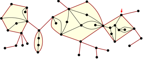
Figure 1: A quadrangulation from ${\bf Q}_{23,19}$. The root is the corner indicated by the red arrow.

Our main result in the context of random quadrangulations is the following.

Theorem 1.

Let $L\in[0,\infty)$ be fixed, and $(l_{n},n\geq 1)$ be a sequence of integers such that $l_{n}/{\sqrt{2n}}\to L$ as $n\to\infty$. Let $Q_{n}$ be uniformly distributed over ${\bf Q}_{l_{n},n}$. There exists a random compact metric space $\mathrm{BD}_{L}$ such that

$$\Big{(}\frac{9}{8n}\Big{)}^{1/4}Q_{n}\mathrel{\mathop{\kern 0.0pt\longrightarrow}\limits_{n\to\infty}^{(d)}}\mathrm{BD}_{L}$$

where the convergence holds in distribution for the Gromov–Hausdorff topology.

The random metric space $\mathrm{BD}_{L}$ is called the Brownian disk with perimeter $L$ and unit area. We will give in Section 2 an explicit description of $\mathrm{BD}_{L}$ (as well as versions with general areas, see also Section 1.5) in terms of certain stochastic processes, and the convention for the scaling constant $(9/8)^{1/4}$ is here to make the description of these processes simpler. The main properties of $\mathrm{BD}_{L}$ are the following; they follow from [10, Theorems 1–3].

Proposition 2.

Let $L>0$ be fixed. Almost surely, the space $\mathrm{BD}_{L}$ is homeomorphic to the closed unit disk of $\mathbb{R}^{2}$. Moreover, almost surely, the Hausdorff dimension of $\mathrm{BD}_{L}$ is $4$, while that of its boundary $\partial\mathrm{BD}_{L}$ is $2$.

We stress that the case $L=0$, corresponding to the situation where $l_{n}=o(\sqrt{n})$, is the statement of [10, Theorem 4], which says that $\mathrm{BD}_{0}$ is the so-called Brownian map. Since the Brownian map is a.s. homeomorphic to the sphere [28], this means that the boundaries of the approximating random maps are too small to be seen in the limit. This particular case generalizes the convergence of uniform random quadrangulations, obtained in [26, 34], corresponding to the case where $l_{n}=2$ for every $n\geq 1$.

The case where $l_{n}/\sqrt{n}\to\infty$ is also of interest, and is the object of [10, Theorem 5], showing that, in this case, $(2l_{n})^{-1/2}Q_{n}$ converges to the so-called Brownian Continuum Random Tree [4, 5]. This means that the boundary takes over the planar geometry and folds the map into a tree-shaped object.

We will prove our result by using the already studied case of plane maps without boundary, together with some surgical methods. Heuristically, we will cut $Q_{n}$ along certain geodesics into elementary pieces of planar topology, to which we can apply a variant of the convergence of random spherical quadrangulations to the Brownian map. The idea of cutting into slices quadrangulations with a boundary along geodesics appears in Bouttier and Guitter [15, 16]. The use of these slices (also called maps with a piecewise geodesic boundary) plays an important role in Le Gall’s approach [26] to the uniqueness of the Brownian map in the planar case, which requires to introduce the scaling limits of these slices. The previously cited works are influential to our approach. It however requires to glue an infinite number of metric spaces along geodesic boundaries, which could create potential problems when passing to the limit.

1.4 Universal aspects of the limit

Another important aspect is that of universality of the spaces $\mathrm{BD}_{L}$. Indeed, we expect these spaces to be the scaling limit of many other models of random maps with a boundary, as in the case of the Brownian map, which corresponds to $L=0$. In the latter case, it has indeed been proved, starting in Le Gall’s work [26], that the Brownian map is the unique scaling limit for a large family of natural models of discrete random maps, see [6, 2, 11, 1]. The now classical approach to universality developed in [26] can be generalized to our context, as we illustrate in the case of critical bipartite Boltzmann maps.

1.4.1 Boltzmann random maps

Let $\mathbf{B}$ be the set of bipartite rooted plane maps, that is, the set of rooted plane maps with faces all having even degrees (equivalently, this is the set of maps whose internal faces all have even degrees). For $l\in\mathbb{Z}_{+}$, let $\mathbf{B}_{l}$ be the set of bipartite maps $\mathbf{m}\in\mathbf{B}$ with perimeter $2l$. Note that when $l=1$, meaning that the root face has degree $2$, there is a natural bijection between $\mathbf{B}_{1}$ and $\mathbf{B}\setminus\mathbf{B}_{0}$, consisting in gluing together the two edges of the root face into one edge.

Let $q=(q_{1},q_{2},\ldots)$ be a sequence of non-negative weights. We assume throughout that $q_{i}>0$ for at least one index $i\geq 2$. The Boltzmann measure associated with the sequence $q$ is the measure $W(q;\cdot)$ on $\mathbf{B}$ defined by

$$W(q;\mathbf{m})=\prod_{f\in\mathbf{F}(\mathbf{m})\setminus\{f_{*}\}}q_{\deg(f)/2}\,.$$

This defines a non-negative, $\sigma$-finite measure, and by convention the vertex-map receives a weight $W(q,\circ)=1$. In what follows, the weight sequence $q$ is considered fixed and its mention will be implicit, so that we denote for example $W(\mathbf{m})=W(q;\mathbf{m})$, and likewise for the variants of $W$ to be defined below.

We aim at understanding various probability measures obtained by conditioning $W$ with respect to certain specific subsets of $\mathbf{B}$. It is a simple exercise to check that $W(\mathbf{B}_{l})$ is non-zero for every $l\in\mathbb{N}$, and that $W(\mathbf{B}_{l})$ is finite for one value of $l>0$ if and only if it is finite for all values of $l>0$. In this case, it makes sense to define the Boltzmann probability measures

$$\mathbb{W}_{l}=W(\cdot\,|\,\mathbf{B}_{l})=\frac{W(\cdot\cap\mathbf{B}_{l})}{W(\mathbf{B}_{l})}\,,\qquad l\geq 0\,.$$

A random map with distribution $\mathbb{W}_{l}$ has a root face of fixed degree $2l$, but a random number of vertices, edges and faces.

Likewise, we can consider conditioned versions of $W$ given both the perimeter and the “size” of the map, where the size can be alternatively the number of vertices, edges or internal faces. We let $\mathbf{B}^{\mathbf{V}}_{l,n}$, $\mathbf{B}^{\mathbf{E}}_{l,n}$, $\mathbf{B}^{\mathbf{F}}_{l,n}$ be the subsets of $\mathbf{B}_{l}$ consisting of maps with respectively $n+1$ vertices, $n$ edges and $n$ internal faces. (The choice of $n+1$ vertices instead of a more natural choice of $n$ vertices is technical and will make the statements simpler.)

In all the statements involving a given weight sequence $q$ and a symbol $\mathbf{S}\in\{\mathbf{V},\mathbf{E},\mathbf{F}\}$ (for “size”), it will always be tacitly imposed that $(l,n)$ belongs to the set

$$\mathcal{E}^{\mathbf{S}}(q)=\{(l,n)\in\mathbb{Z}_{+}^{2}:W(\mathbf{B}^{\mathbf{S}}_{l,n})>0\}\,.$$

Note that for $(l,n)\in\mathcal{E}^{\mathbf{S}}(q)$, it holds that $W(\mathbf{B}^{\mathbf{S}}_{l,n})<\infty$ since $W(\mathbf{B}_{l})<\infty$. In this way, we can define the distribution

$$\mathbb{W}^{\mathbf{S}}_{l,n}(\cdot)=W(\cdot\,|\,\mathbf{B}^{\mathbf{S}}_{l,n})\,.$$

It will be useful in the following to know what the set $\mathcal{E}^{\mathbf{S}}(q)$ looks like. More precisely, let

$$\mathcal{E}^{\mathbf{S}}_{l}(q)=\{n\geq 0:(l,n)\in\mathcal{E}^{\mathbf{S}}(q)\}\,.$$ (1)

As above, when the weight sequence $q$ is unequivocally fixed, we will drop the mention of it from the notation and write $\mathcal{E}^{\mathbf{S}}$ and $\mathcal{E}^{\mathbf{S}}_{l}$.

Define three numbers $h^{\mathbf{V}}$, $h^{\mathbf{E}}$, $h^{\mathbf{F}}$ by

$$h^{\mathbf{V}}=\mathrm{gcd}(\{n\geq 2:q_{2n}>0\})\,,\qquad h^{\mathbf{E}}=\mathrm{gcd}(\{n\geq 1:q_{2n}>0\})\,,\qquad h^{\mathbf{F}}=1\,.$$ (2)

Then we have the following lemma, which is a slight generalization of [38, Section 6.3.1].

Lemma 3.

Let $q$ be a weight sequence, and let $\mathbf{S}$ be one of the three symbols $\mathbf{V}$, $\mathbf{E}$, $\mathbf{F}$. There exists an integer $\beta^{\mathbf{S}}\geq 0$ such that for every $l\geq 1$, there exists a set $R^{\mathbf{S}}_{l}\subseteq\{0,1,\ldots,l\beta^{\mathbf{S}}-1\}$ such that

$$\mathcal{E}^{\mathbf{S}}_{l}(q)=R^{\mathbf{S}}_{l}\cup(l\beta^{\mathbf{S}}+h^{\mathbf{S}}\mathbb{Z}_{+})\,.$$

In fact, note that $\mathcal{E}^{\mathbf{F}}_{l}(q)=\mathbb{Z}_{+}$, which amounts to the fact that, for any $q$ and any $n\geq 0$, $l\geq 1$, there is at least one map $\mathbf{m}$ with $n$ internal faces and perimeter $2l$ such that $W(q;\mathbf{m})>0$. As a consequence, we can always take $\beta^{\mathbf{F}}=0$.

1.4.2 Admissible, regular critical weight sequences

Let us introduce some terminology taken from [30]. Let

$$f_{q}(x)=\sum_{k\geq 0}x^{k}\binom{2k+1}{k}q_{k+1}\,,\qquad x\geq 0\,.$$

This defines a totally monotone function with values in $[0,\infty]$.

Definition 4.

We say that $q$ is admissible if the equation

$$f_{q}(z)=1-\frac{1}{z}$$ (3)

admits a solution $z>1$. We also say that $q$ is regular critical if moreover this solution satisfies

$$z^{2}f_{q}^{\prime}(z)=1$$

and if there exists $\varepsilon>0$ such that $f_{q}(z+\varepsilon)<\infty$.

Note that $q$ being regular critical means that the graphs of $f_{q}$ and of $x\mapsto 1-1/x$ are tangent at the point of abscissa $z$, and in particular, by convexity of $f_{q}$, the solution $z$ to (3) is unique. We denote by

$$\mathcal{Z}_{q}=z$$

this solution, which will play an important role in the discussion to come.

To give a little more insight into this definition, let us introduce at this point a measure on maps that looks less natural at first sight than the Boltzmann measure $\mathbb{W}_{l}$, but which will turn out to be better-behaved from the bijective point of view on which this work relies. Let $\mathbf{B}^{\bullet}$ be the set of pairs $(\mathbf{m},v_{*})$ where $\mathbf{m}\in\mathbf{B}$ is a rooted bipartite map and $v_{*}\in\mathbf{V}(\mathbf{m})$ is a distinguished vertex. We also let $\mathbf{B}^{\bullet}_{l}$ be the subset of $\mathbf{B}^{\bullet}$ consisting of the maps having perimeter $2l$. We let $W^{\bullet}(q;\cdot)$ be the measure on $\mathbf{B}^{\bullet}$ defined by

$$W^{\bullet}(q;\{(\mathbf{m},v_{*})\})=W(\mathbf{m})\,,\qquad(\mathbf{m},v_{*})\in\mathbf{B}^{\bullet}\,,$$ (4)

as well as the probability measures $\mathbb{W}^{\bullet}$ and $\mathbb{W}^{\bullet}_{l}$, defined by conditioning $W^{\bullet}$ respectively on $\mathbf{B}^{\bullet}$ and $\mathbf{B}^{\bullet}_{l}$. Note that, if $\phi(\mathbf{m},v_{*})=\mathbf{m}$ denotes the map from $\mathbf{B}^{\bullet}$ to $\mathbf{B}$ that forgets the marked point, then $\mathbb{W}_{l}$ is absolutely continuous with respect to $\phi_{*}\mathbb{W}^{\bullet}_{l}$, with density function given by

$$\mathrm{d}\mathbb{W}_{l}(\mathbf{m})=\frac{K_{l}}{|\mathbf{V}|}\mathrm{d}(\phi_{*}\mathbb{W}^{\bullet}_{l})(\mathbf{m})\,,$$ (5)

where $|\mathbf{V}|$ should be understood as the random variable $\mathbf{m}\mapsto|\mathbf{V}(\mathbf{m})|$ giving the number of vertices of the map, and $K_{l}=\mathbb{W}^{\bullet}_{l}[1/|\mathbf{V}|]^{-1}$. This fact will be useful later.

Proposition 1 in [30] shows that the sequence $q$ of non-negative weights is admissible if and only if $W^{\bullet}(q;\mathbf{B}^{\bullet}_{1})<\infty$ (this is in fact the defining condition of admissibility in [30]). We see that this clearly implies that $W(q;\mathbf{B}_{1})<\infty$, and even that $W(q;\mathbf{B}_{l})<\infty$ for every $l\geq 1$. Moreover, in this case, the constant $\mathcal{Z}_{q}$ has a nice interpretation in terms of the pointed measures. Namely, it holds that

$$\mathcal{Z}_{q}=1+W^{\bullet}(\mathbf{B}^{\bullet}_{1})/2\,.$$ (6)

From now on, our attention will be exclusively focused on regular critical weight sequences. It is not obvious at this point how to interpret the definition, which will become clearer when we see how to code maps with decorated trees. However, let us explain now in which context this property typically intervenes, and refer the reader to the upcoming Subsection 1.4.3 for two applications. For instance, if one wants to study uniform random quadrangulations with a boundary and with $n$ faces as we did in the first part of this paper, it is natural to consider the sequence $q^{\circ}=\delta_{2}=(0,1,0,0,\ldots)$ and to note that $\mathbb{W}^{\mathbf{F}}_{l,n}(q^{\circ};\cdot)$ is the uniform distribution on ${\bf Q}_{l,n}$. Here, note that the sequence $q^{\circ}$ is not admissible, but the probability measure $\mathbb{W}^{\mathbf{F}}_{l,n}(q^{\circ};\cdot)$ does make sense because $0<W(\mathbf{B}^{\mathbf{F}}_{l,n})<\infty$, due to the fact that there are finitely many quadrangulations with a boundary of perimeter $2l$, and with $n$ internal faces. Now, it can be checked that $q=12^{-1}q^{\circ}$ is admissible and regular critical, and that $\mathbb{W}^{\mathbf{F}}_{l,n}(q;\cdot)=\mathbb{W}^{\mathbf{F}}_{l,n}(q^{\circ};\cdot)$ is still the uniform distribution on ${\bf Q}_{l,n}$. This way of transforming a “naturally given” weight sequence $q^{\circ}$ into a regular weight sequence while leaving $\mathbb{W}^{\mathbf{S}}_{l,n}$ invariant is common and very useful.

The main result is the following. Let $q$ be a regular critical weight sequence. Define $\rho_{q}=2+\mathcal{Z}_{q}^{3}f^{\prime\prime}_{q}(\mathcal{Z}_{q})$ and let ${\sigma_{\mathbf{E}}}$, ${\sigma_{\mathbf{V}}}$, ${\sigma_{\mathbf{F}}}$ be the non-negative numbers with squares

$${\sigma_{\mathbf{E}}}^{2}=\frac{\rho_{q}}{\mathcal{Z}_{q}}\,,\quad{\sigma_{\mathbf{V}}}^{2}=\rho_{q}\,,\quad{\sigma_{\mathbf{F}}}^{2}=\frac{\rho_{q}}{\mathcal{Z}_{q}-1}\,.$$ (7)

For $L>0$, we denote by $\mathscr{S}^{\mathbf{S}}_{L}$ the set of sequences $(l_{k},n_{k})_{k\geq 0}\in(\mathcal{E}^{\mathbf{S}})^{\mathbb{N}}$ such that $l_{k}$, $n_{k}\to\infty$ with $l_{k}\sim L{\sigma_{\mathbf{S}}}\sqrt{n_{k}}$ as $k\to\infty$.

Theorem 5.

Let $\mathbf{S}$ denote one of the symbols $\mathbf{V}$, $\mathbf{E}$, $\mathbf{F}$, and $(l_{k},n_{k})_{k\geq 0}\in\mathscr{S}^{\mathbf{S}}_{L}$ for some $L>0$. For $k\geq 0$, denote by $M_{k}$ a random map with distribution $\mathbb{W}^{\mathbf{S}}_{l_{k},n_{k}}$. Then

$$\left(\frac{4{\sigma_{\mathbf{S}}}^{2}}{9}\,n_{k}\right)^{-1/4}M_{k}\mathrel{\mathop{\kern 0.0pt\longrightarrow}\limits_{k\to\infty}^{(d)}}\mathrm{BD}_{L}$$

in distribution for the Gromov–Hausdorff topology.

Remark 1.

The intuitive meaning for these renormalization constants is the following: in a large random map with Boltzmann distribution, it can be checked that the numbers $|\mathbf{V}|$ and $|\mathbf{F}|$ of vertices and faces are of order $|\mathbf{E}|/\mathcal{Z}_{q}$ and $|\mathbf{E}|(1-1/\mathcal{Z}_{q})$ respectively, where $|\mathbf{E}|$ is the number of edges, and that conditioning on having $n$ edges is asymptotically the same as conditioning on having (approximately) $n/\mathcal{Z}_{q}$ vertices, or $n\,(1-1/\mathcal{Z}_{q})$ faces.

Remark 2.

In fact, the above result is also valid in the case where $L=0$, with the interpretation that $\mathrm{BD}_{0}$ is the Brownian map. The proof of this claim can be obtained by following ideas similar to [10, Section 6.1]. However, a full proof requires the convergence of a map with law $\mathbb{W}_{1,n}^{\mathbf{S}}$, rescaled by $(4{\sigma_{\mathbf{S}}}^{2}n/9)^{1/4}$, to the Brownian map, and this has been explicitly done only in the case where $\mathbf{S}=\mathbf{V}$ in [26, Section 9]. In fact, building on the existing literature [30, 32], it is easy to adapt the argument to work for $\mathbf{S}=\mathbf{F}$ in the same way, while the case $\mathbf{S}=\mathbf{E}$, which is slightly different, can be tackled by the methods of [1]. Writing all the details would add a consequent number of pages to this already lengthy paper, so we will omit the proof.

1.4.3 Applications

Let us give two interesting specializations of Theorem 5. If $p\geq 2$ is an integer, a $2p$-angulation with a boundary is a map whose internal faces all have degree $2p$. The computations of the various constants appearing in the statement of Theorem 5 have been performed in Section 1.5.1 of [30]. These show that the weight sequence

$$q=\frac{(p-1)^{p-1}}{p^{p}\binom{2p-1}{p}}\delta_{p}$$

is regular critical, that $\mathbb{W}^{\mathbf{F}}_{l,n}$ is the uniform law on the set of $2p$-angulations with $n$ faces and perimeter $2l$ in this case, and that the constants are

$$\mathcal{Z}_{q}=\frac{p}{p-1}\,,\quad\rho_{q}=p\,,\quad{\sigma_{\mathbf{E}}}^{2}=p-1\,,\quad{\sigma_{\mathbf{V}}}^{2}=p\,,\quad{\sigma_{\mathbf{F}}}^{2}=p(p-1)\,.$$

Therefore, in this situation, Theorem 5 for $\mathbf{S}=\mathbf{F}$ gives the following result, that clearly generalizes Theorem 1.

Corollary 6.

Let $L\in(0,\infty)$ be fixed, $(l_{n},n\geq 1)$ be a sequence of integers such that $l_{n}\sim L\sqrt{p(p-1)n}$ as $n\to\infty$, and $M_{n}$ be uniformly distributed over the set of $2p$-angulations with $n$ internal faces and with perimeter $2l_{n}$. Then the following convergence holds in distribution for the Gromov–Hausdorff topology:

$$\Big{(}\frac{9}{4p(p-1)\,n}\Big{)}^{1/4}M_{n}\mathrel{\mathop{\kern 0.0pt\longrightarrow}\limits_{n\to\infty}^{(d)}}\mathrm{BD}_{L}.$$

Next, consider the case where $q_{k}=a^{-k}$, $k\geq 1$ for some $a>0$. In this case, for every $\mathbf{m}\in\mathbf{B}$, a simple computation shows that

$$W(\mathbf{m})=a^{-|\mathbf{E}(\mathbf{m})|+l}$$

so that $\mathbb{W}^{\mathbf{E}}_{l,n}$ is the uniform distribution over bipartite maps with $n$ edges and a perimeter $2l$. It was shown in [30, Section 1.5.2] (and implicitly recovered in [1, Proposition 2]) that choosing $a=1/8$ makes $q$ regular critical and that, in this case,

$$\mathcal{Z}_{q}=\frac{3}{2}\,,\qquad\rho_{q}=\frac{27}{4}\,,\qquad{\sigma_{\mathbf{E}}}^{2}=\frac{9}{2}\,.$$

Thus, one deduces the following statement, that should be compared to [1, Theorem 1].

Corollary 7.

Let $M_{n}$ be a uniform random bipartite map with $n$ edges and with perimeter $2l_{n}$, where $l_{n}\sim 3L\sqrt{n/2}$ for some $L>0$. Then the following convergence holds in distribution for the Gromov–Hausdorff topology:

$$(2n)^{-1/4}M_{n}\mathrel{\mathop{\kern 0.0pt\longrightarrow}\limits_{n\to\infty}^{(d)}}\mathrm{BD}_{L}.$$

1.5 Convergence of Boltzmann maps

The models we have presented so far consist in taking a random map with a fixed size and perimeter and letting both these quantities go to infinity in an appropriate regime. However, it is legitimate to ask about the behavior of a typical random map with law $\mathbb{W}_{l}$ or $\mathbb{W}^{\bullet}_{l}$ when $l\to\infty$, so that the perimeter is fixed and large, while the total size is left free.

For every $L\geq 0$ and $A>0$, we define a random metric space $\mathrm{BD}_{L,A}$, which we interpret as the Brownian disk with area $A$ and perimeter $L$. For concreteness, the space $\mathrm{BD}_{L,A}$ has same distribution as $A^{1/4}\,\mathrm{BD}_{A^{-1/2}L}$. To motivate the definition, note that $\mathrm{BD}_{L,1}$ has same distribution as $\mathrm{BD}_{L}$ and that if $Q_{n}$ is a uniform random element in ${\bf Q}_{\lfloor L\sqrt{2n}\rfloor,\lfloor An\rfloor}$, then $(8n/9)^{-1/4}Q_{n}$ converges in distribution for the Gromov–Hausdorff topology to $\mathrm{BD}_{L,A}$ by virtue of Theorem 1. See also Remark 3 in Section 2.3 below.

Let $\mathcal{A}^{\bullet}$ be a stable random variable with index $1/2$, with distribution given by

$$\mathbb{P}(\mathcal{A}^{\bullet}\in\mathrm{d}A)=\frac{1}{\sqrt{2\pi A^{3}}}\exp\left(-\frac{1}{2A}\right)\mathrm{d}A\,\mathbf{1}_{\{A>0\}}\,.$$

Note that $\mathbb{E}[1/\mathcal{A}^{\bullet}]=1$, so that the formula

$$\frac{\mathbb{P}(\mathcal{A}^{\bullet}\in\mathrm{d}A)}{A}=\frac{1}{\sqrt{2\pi A^{5}}}\exp\left(-\frac{1}{2A}\right)\mathrm{d}A\,\mathbf{1}_{\{A>0\}}$$

also defines a probability distribution, and we let $\mathcal{A}$ be a random variable with this distribution. We define the free Brownian disk with perimeter $1$ to be a space with same law as $\mathrm{BD}_{1,\mathcal{A}}$, where this notation means that conditionally given $\mathcal{A}=A$, it has same distribution as $\mathrm{BD}_{1,A}$. Likewise, the free pointed Brownian disk with perimeter $1$ has same distribution as $\mathrm{BD}_{1,\mathcal{A}^{\bullet}}$.

For future reference, for $L>0$, it is natural to define the law of the free Brownian disk (resp. free pointed Brownian disk) with perimeter $L$ by scaling, setting it to be the law of $\sqrt{L}\,\mathrm{BD}_{1,\mathcal{A}}$ or equivalently of $\mathrm{BD}_{L,L^{2}\mathcal{A}}$ (resp. $\sqrt{L}\,\mathrm{BD}_{1,\mathcal{A}^{\bullet}}=^{(d)}\mathrm{BD}_{L,L^{2}\mathcal{A}^{\bullet}}$). We let $\mathrm{FBD}_{L}$ (resp. $\mathrm{FBD}^{\bullet}_{L}$) stand for the free Brownian disk (resp. free pointed Brownian disk) with perimeter $L$.

Theorem 8.

Let $q$ be a regular critical weight sequence. For $l\in\mathbb{N}$, let $B_{l}$ (resp. $B^{\bullet}_{l}$) be distributed according to $\mathbb{W}_{l}(q;\cdot)$ (resp. $\mathbb{W}^{\bullet}_{l}(q;\cdot)$). Then

$$\left(\frac{2l}{3}\right)^{-1/2}B_{l}\mathrel{\mathop{\kern 0.0pt\longrightarrow}\limits_{l\to\infty}^{(d)}}\mathrm{FBD}_{1}$$

and respectively

$$\left(\frac{2l}{3}\right)^{-1/2}B^{\bullet}_{l}\mathrel{\mathop{\kern 0.0pt\longrightarrow}\limits_{l\to\infty}^{(d)}}\mathrm{FBD}^{\bullet}_{1}$$

in distribution for the the Gromov–Hausdorff topology.

It is remarkable that the renormalization in this theorem does not involve $q$ whatsoever!

1.6 Further comments and organization of the paper

The very recent preprint [35] by Miller and Sheffield aims at providing an axiomatic characterization of the Brownian map in terms of elementary properties. In this work, certain measures on random disks play a central role. We expect that these measures, denoted by $\mu_{\mathrm{DISK}}^{k,L}$ for $k\in\{0,1\}$ and $L>0$, are respectively the laws of the free Brownian disk ($k=0$) and the pointed free Brownian disk ($k=1$) with perimeter $L>0$. Miller and Sheffield define these measures directly in terms of the metric balls in certain versions of the Brownian map, and it is not immediate, though it is arguably very likely, that this definition matches the one given in the present paper. Establishing such a connection would be interesting from the perspective of [35] since, for example, it is not established that $\mu_{\mathrm{DISK}}^{k,L}$ is supported on compact metric spaces, due to the possibly wild behavior of the boundary from a metric point of view. We hope to address such questions in future work.

Note also that [35] introduces another measure on metric spaces, called $\mu_{\mathrm{MET}}^{L}$, which intuitively corresponds to the law of a variant of a metric ball in the Brownian map, with a given boundary length. A description of this measure in terms of slices is given in [35], which is very much similar to the one we describe in the current work. However, there is a fundamental difference, which is that $\mu_{\mathrm{MET}}^{L}$ does not satisfy the invariance under re-rooting that is essential to our study of random disks. In a few words, in a random disk with distribution $\mu_{\mathrm{MET}}^{L}$, all points of the boundary are equidistant from some special point (the center of the ball), while it is very likely that no such point exists a.s. in $\mathrm{BD}_{L,A}$, or under the law $\mu_{\mathrm{DISK}}^{k,L}$.

It would be natural to consider the operation that consists in gluing Brownian disks, say with same perimeter, along their boundaries, hence constructing what should intuitively be a random sphere with a self-avoiding loop. However, this operation is in general badly behaved from a metric point of view (in the sense of [17, Chapter 3] say), and it is not clear that the resulting space has the same topology as the topological gluing. The reason for this difficulty is that we require to glue along curves that are not Lipschitz, since the boundaries of the spaces $\mathrm{BD}_{L}$ have Hausdorff dimension $2$ (by contrast, the gluings considered in Section 5 of the present paper are all along geodesics.) At present, such questions remain to be investigated.

The rest of the paper is organized as follows. In Section 2, we give a self-standing definition of the limiting objects. As in many papers on random maps, we rely on bijective tools, and Section 3 introduces these tools. Section 4 gives a technical result of convergence of slices, which are the elementary pieces from which the Brownian disks are constructed. Section 5 is dedicated to the proof of Theorem 1. In Sections 6–8, we address the question of universality and prove Theorems 5 and 8.

Acknowledgments. This work is partly supported by the GRAAL grant ANR-14-CE25-0014. We also acknowledge partial support from the Isaac Newton Institute for Mathematical Sciences where part of this work was conducted, and where G.M. benefited from a Rothschild Visiting Professor position during January 2015.

We thank Erich Baur, Timothy Budd, Guillaume Chapuy, Nicolas Curien, Igor Kortchemski, Jean-François Le Gall, Jason Miller, Gourab Ray and Scott Sheffield, for useful remarks and conversations during the elaboration of this work.

2 Definition of Brownian disks

Recall that the Brownian map $\mathrm{BD}_{0}$ is defined ([24], see also [31] and Section 4.1 below) in terms of a certain stochastic process called the normalized Brownian snake. Likewise, the spaces $\mathrm{BD}_{L}$, $L>0$ of Theorem 1 are defined in terms of stochastic processes, as we now discuss.

2.1 First-passage bridges and random continuum forests

The first building blocks of the Brownian disks are first-passage bridges of Brownian motion. Informally, given $A$, $L>0$, the first-passage bridge at level $-L$ and time $A$ is a Brownian motion conditioned to first hit $-L$ at time $A$. To be more precise, let us introduce some notation. We let $X$ be the canonical continuous process, and $\mathcal{G}_{s}=\sigma(X_{u},u\leq s)$ be the associated canonical filtration. Denote by $\mathbb{P}$ the law of standard Brownian motion, and by $\mathbb{P}^{A}$ the law of standard Brownian motion killed at time $A>0$. For $L\geq 0$, let $T_{L}=\inf\{s\geq 0:X_{s}=-L\}$ be the first hitting time of $-L$. We denote the density function of its law by

$$j_{L}(A)=\frac{\mathbb{P}(T_{L}\in\mathrm{d}A)}{\mathrm{d}A}=\frac{L}{\sqrt{2\pi A^{3}}}\exp\left(-\frac{L^{2}}{2A}\right)\,.$$ (8)

With this notation, the law $\mathbb{F}^{A}_{L}$ of the first-passage bridge at level $-L$ and at time $A$ can informally be seen as $\mathbb{P}^{A}(\,\cdot\,|\,T_{L}=A)$. It is best defined by an absolute continuity relation with respect to $\mathbb{P}^{A}$. Namely, for every $s\in(0,A)$ and every non-negative random variable $G$ that is measurable with respect to $\mathcal{G}_{s}$, we let

$$\mathbb{F}^{A}_{L}(G)=\mathbb{P}^{A}\left[G\,\mathbf{1}_{\{T_{L}>s\}}\frac{j_{L+X_{s}}(A-s)}{j_{L}(A)}\right]\,.$$ (9)

It can be seen [18] that this definition is consistent and uniquely extends to a law $\mathbb{F}^{A}_{L}$ on $\mathcal{G}_{A}$, supported on continuous processes, and for which $\mathbb{F}^{A}_{L}(T_{L}=A)=1$.

An alternative description of first-passage bridges, which will be useful to us later, is the following.

Proposition 9.

Let $A$, $L>0$. Then for every $y\in(0,L)$ and for every non-negative random variable $G$ that is measurable with respect to $\mathcal{G}_{T_{y}}$, we have

$$\mathbb{F}^{A}_{L}[G]=\mathbb{P}^{A}\left[G\,\mathbf{1}_{\{T_{y}<A\}}\frac{j_{L-y}(A-T_{y})}{j_{L}(A)}\right]\,.$$ (10)

Moreover, this property characterizes $\mathbb{F}^{A}_{L}$ among all measures on $\mathcal{G}_{A}$ supported on continuous functions.

Proof.

The definition of $\mathbb{F}^{A}_{L}$ implies that the process $\mathcal{M}=(\mathbf{1}_{\{T_{L}>s\}}j_{L+X_{s}}(A-s)/j_{L}(A),\,0\leq s<A)$ is a $(\mathcal{G}_{s},\,0\leq s<A)$-martingale. Therefore, for every stopping time $T$ such that $T<A$ a.s. under $\mathbb{F}^{A}_{L}$, and for every $E\in\mathcal{G}_{T}$, we have

$$\mathbb{F}_{L}^{A}(E)=\lim_{s\uparrow A}\mathbb{P}^{A}[\mathbf{1}_{E\cap\{T\leq s\}}\mathcal{M}_{s}]=\lim_{s\uparrow A}\mathbb{P}^{A}[\mathbf{1}_{E\cap\{T\leq s\}}\mathbb{P}^{A}[\mathcal{M}_{s}\,|\,\mathcal{G}_{T}]]=\lim_{s\uparrow A}\mathbb{P}^{A}[\mathbf{1}_{E\cap\{T\leq s\}}\mathcal{M}_{T}]\,,$$

and this is equal to $\mathbb{P}^{A}[\mathbf{1}_{E}\mathcal{M}_{T}]$. The formula is obtained by applying this result to $T=T_{y}$, and by a standard approximation procedure of a general measurable function by weighted sums of indicator functions.

The fact that $\mathbb{F}^{A}_{L}$ is characterized by these formulas comes from the following observation. Define $\tilde{\mathbb{F}}^{A}_{L}$ on $\mathcal{G}_{T_{y}}$ as being absolutely continuous with respect to $\mathbb{P}^{A}|_{\mathcal{G}_{T_{y}}}$, with density $\mathcal{M}_{T_{y}}$. Then for every $s<A$, $\tilde{\mathbb{F}}^{A}_{L}(T_{y}<s)=\mathbb{P}^{A}[\mathbf{1}_{\{T_{y}<s\}}j_{L-y}(A-T_{y})/j_{L}(A)]$, and this clearly converges to $0$ as $y\uparrow L$. Therefore, $T_{y}$ converges $\tilde{\mathbb{F}}^{A}_{L}$-a.s. to $A$ as $y\uparrow L$. Then for every $s<A$ and $E\in\mathcal{G}_{s}$, similar manipulations to the above ones show that

$$\tilde{\mathbb{F}}^{A}_{L}(E)=\lim_{y\uparrow L}\tilde{\mathbb{F}}^{A}_{L}(E\cap\{T_{y}>s\})=\lim_{y\uparrow L}\mathbb{P}^{A}\left[\mathbf{1}_{E\cap\{T_{y}>s\}}\mathcal{M}_{T_{y}}\right]=\lim_{y\uparrow L}\mathbb{P}^{A}\left[\mathbf{1}_{E\cap\{T_{y}>s\}}\mathcal{M}_{s}\right]$$

and this is $\lim_{y\uparrow L}\mathbb{F}^{A}_{L}(E\cap\{T_{y}>s\})=\mathbb{F}^{A}_{L}(E)$. ∎

It is convenient to view a first-passage bridge as encoding a random continuum forest. This is a classical construction that can be summarized as follows, see for instance [36]. Here we work under $\mathbb{F}^{A}_{L}$. For $0\leq s\leq s^{\prime}\leq A$, define $\underline{X}_{s,s^{\prime}}=\inf\{X_{u}:s\leq u\leq s^{\prime}\}$ and let

$$d_{X}(s,s^{\prime})=X_{s}+X_{s^{\prime}}-2\underline{X}_{s\wedge s^{\prime},s\vee s^{\prime}}\qquad s,s^{\prime}\in[0,A].$$ (11)

The function $d_{X}$ on $[0,A]^{2}$ is a pseudo-metric, to which one can associate a random metric space $\mathcal{F}^{A}_{L}=[0,A]/\{d_{X}=0\}$, endowed with the quotient metric induced from $d_{X}$. This metric space is a.s. a compact $\mathbb{R}$-tree, that is, a compact geodesic metric space into which $\mathbb{S}^{1}$ cannot be embedded. It comes with a distinguished geodesic of length $L$, which is the image of the first hitting times $\{T_{y},0\leq y\leq L\}$ under the canonical projection $p_{X}:[0,A]\to\mathcal{F}^{A}_{L}$. It is convenient to view this segment as the floor of a forest of $\mathbb{R}$-trees, these trees being exactly of the form $\mathcal{T}_{y}=p_{X}((T_{y-},T_{y}])$, corresponding to the excursions of $X$ above its past infimum. One should imagine that the $\mathbb{R}$-tree $\mathcal{T}_{y}$ is grafted at the point $p_{X}(T_{y})$ of the floor lying at distance $y$ from $p_{X}(0)$.

2.2 Snakes

We now enrich the random “real forest” described above by assigning labels to it. Informally speaking, the trees of the forest are labeled by independent Brownian snakes [23, 21], while the floor of the forest is labeled by a Brownian bridge with variance factor $3$.

More precisely, let $X$ be a first-passage bridge with law $\mathbb{F}^{A}_{L}$. Conditionally given $X$, we let $(Z^{\mathbf{0}}_{s},0\leq s\leq A)$ be a centered Gaussian process with covariance function

$${\rm Cov\,}(Z^{\mathbf{0}}_{s},Z^{\mathbf{0}}_{s^{\prime}})=\inf_{u\in[s\wedge s^{\prime},s\vee s^{\prime}]}(X_{u}-\underline{X}_{u})\qquad s,s^{\prime}\in[0,A]\,,$$ (12)

where $\underline{X}_{u}=\inf_{0\leq v\leq u}X_{v}$ is the past infimum of $X$. Note in particular that $Z^{\mathbf{0}}_{s}$ and $Z^{\mathbf{0}}_{s^{\prime}}$ are independent if $s$, $s^{\prime}$ belong to two different excursion intervals of $X$ above $\underline{X}$. It is classical [23] that $Z^{\mathbf{0}}$ admits a continuous modification, see also [7] for a discussion in the current context. For this modification, we a.s. have $Z^{\mathbf{0}}_{T_{y}}=0$ for every $y\in[0,L]$ (for a given $y$, this comes directly from the variance formula). The process $Z^{\mathbf{0}}$ is sometimes called the head of the Brownian snake driven by the process $X-\underline{X}$, the reason being that it can be obtained as a specialization of a path-valued Markov process called the Brownian snake [23] driven by $X-\underline{X}$. The process $Z^{\mathbf{0}}$ itself is not Markov.

Let also $\mathrm{b}$ be a standard Brownian bridge of duration $L$, so that

$${\rm Cov\,}(\mathrm{b}_{y},\mathrm{b}_{y^{\prime}})=\frac{y(L-y^{\prime})}{L}\,,\qquad 0\leq y\leq y^{\prime}\leq L\,.$$

We define the process $Z$ to be

$$Z_{s}=Z^{\mathbf{0}}_{s}+\sqrt{3}\,\mathrm{b}_{T^{-1}(s)}\,,\qquad 0\leq s\leq A\,,$$ (13)

where $T^{-1}(s)=\sup\{y\geq 0:T_{y}\leq s\}$. We abuse notation and still denote by $\mathbb{F}^{A}_{L}$ the law of the pair $(X,Z)$ thus defined, so that $\mathbb{F}^{A}_{L}$ is seen as a probability distribution on the space $\mathcal{C}([0,A],\mathbb{R})^{2}$. In the same spirit, we will still denote by $\mathcal{G}_{t}$ the natural filtration $\sigma(\{(X_{s},Z_{s}),\,0\leq s\leq t\})$. Note that the absolute continuity relations (9) and (10) are still valid verbatim with these extended notation and, in particular, the density function involves only $X$ and not $Z$.

It is classical that a.s. under $\mathbb{F}^{A}_{L}$, $Z$ is a class function on $[0,A]$ for the equivalence relation $\{d_{X}=0\}$, so that $Z$ can also be seen as a function on the forest $\mathcal{F}^{A}_{L}$. Note that $T^{-1}(T_{y})=y$ for every $0\leq y\leq L$, which corresponds to the fact that, in the above depiction of the random forest, the point $p_{X}(T_{y})$ receives label $\sqrt{3}\,\mathrm{b}_{y}$.

It is a simple exercise to check that the above definition of $Z$ is equivalent to the following quicker (but more obscure) one. Conditionally given $X$, we have that $Z$ is Gaussian, centered, with covariance function

$${\rm Cov\,}(Z_{s},Z_{s^{\prime}})=\underline{X}_{s,s^{\prime}}-\underline{X}_{s^{\prime}}-3\underline{X}_{s}(L+\underline{X}_{s^{\prime}})/L\qquad s,s^{\prime}\in[0,A]\,.$$

Similarly as (11), we define a pseudo-metric using the process $Z$ instead of $X$, but with an extra twist. As above, let $\underline{Z}_{s,s^{\prime}}=\inf\{Z_{u}:u\in[s,s^{\prime}]\}$ for $0\leq s\leq s^{\prime}\leq A$, and this time we extend the definition to $0\leq s^{\prime}<s\leq A$ by setting

$$\underline{Z}_{s,s^{\prime}}=\inf\{Z_{u}:u\in[s,A]\cup[0,s^{\prime}]\}=\underline{Z}_{s,A}\wedge\underline{Z}_{0,s^{\prime}}\,,$$

so if we see $[0,A]$ as a circle by identifying $0$ with $A$, $\underline{Z}_{s,s^{\prime}}$ is the minimum of $Z$ on the directed arc from $s$ to $s^{\prime}$. We let

$$d_{Z}(s,s^{\prime})=Z_{s}+Z_{s^{\prime}}-2\max(\underline{Z}_{s,s^{\prime}},\underline{Z}_{s^{\prime},s})\qquad s,s^{\prime}\in[0,A]\,.$$ (14)

2.3 Brownian disks

We are now ready to give the definition of Brownian disks. Consider the set $\mathcal{D}$ of all pseudo-metrics $d$ on $[0,A]$ satisfying the two properties

$$\left\{\begin{array}[]{c}\{d_{X}=0\}\subseteq\{d=0\}\\ d\leq d_{Z}\,.\end{array}\right.$$

The set $\mathcal{D}$ is nonempty (it contains the zero pseudo-metric) and contains a maximal element $D^{*}$ defined by

$$D^{*}(s,s^{\prime})=\inf\left\{\sum_{i=1}^{k}d_{Z}(s_{i},t_{i}):\begin{array}[]{l}k\geq 1\,,\quad t_{1},s_{2},\ldots,s_{k}\in[0,A],\,s_{1}=s,\,t_{k}=s^{\prime},\\ d_{X}(t_{i},s_{i+1})=0\,\mbox{ for every }i\in\{1,\ldots,k-1\}\end{array}\right\}\,,$$ (15)

see [17, Chapter 3]. The Brownian disk $\mathrm{BD}_{L,A}$ with area $A$ and perimeter $L$ is the quotient set $[0,A]/\{D^{*}=0\}$, endowed with the quotient metric induced from $D^{*}$ (which we still denote by $D^{*}$ for simplicity), and considered under the law $\mathbb{F}^{A}_{L}$. In the case $A=1$, we drop the second subscript and write $\mathrm{BD}_{L}=\mathrm{BD}_{L,1}$.

Remark 3.

Observe that, by usual scaling properties of Gaussian random variables, under the law $\mathbb{F}^{A}_{L}$, the scaled pair $((\lambda^{1/2}X_{s/\lambda},\,0\leq s\leq\lambda A),(\lambda^{1/4}Z_{s/\lambda},\,0\leq s\leq\lambda A))$ has law $\mathbb{F}^{\lambda A}_{\lambda^{1/2}L}$, from which we deduce that the random metric space $\lambda^{-1/4}\mathrm{BD}_{\lambda^{1/2}\,L,\lambda A}$ has the same distribution as $\mathrm{BD}_{L,A}$.

The reason why we say that $\mathrm{BD}_{L,A}$ has “area” $A$ is that it naturally comes with a non-negative measure of total mass $A$, which is the image of the Lebesgue measure on $[0,A]$ by the canonical projection $\mathbf{p}:[0,A]\to\mathrm{BD}_{L,A}$. It will be justified later that $\mathrm{BD}_{L,A}$ is a.s. homeomorphic to the closed unit disk, so that the term area makes more sense in this context. Furthermore, the boundary $\partial\mathrm{BD}_{L,A}$ will be shown to be equal to $\mathbf{p}(\{T_{y}:0\leq y\leq L\})$, so that it can be endowed with a natural non-negative measure with total mass $L$, which is the image of the Lebesgue measure on $[0,L]$ by $y\mapsto\mathbf{p}(T_{y})$. This justifies the term “perimeter”.

3 The Schaeffer bijection and two variants

This work strongly relies on powerful encodings of discrete maps by trees and related objects. In this section we present the encodings we will need: the original Cori–Vauquelin–Schaeffer bijection [19, 37], a variant for so-called slices [26] and a variant for plane quadrangulations with a boundary (particular case of [14]). We only give the constructions from the encoding objects to the considered maps and refer the reader to the aforementioned works for converse constructions and proofs.

3.1 The original Cori–Vauquelin–Schaeffer bijection

Let $(\mathbf{t},\ell)$ be a well-labeled tree with $n$ edges. Recall that this means that $\mathbf{t}$ is a rooted plane tree with $n$ edges, and $\ell:\mathbf{V}(\mathbf{t})\to\mathbb{Z}$ is a labeling function such that $\ell(u)-\ell(v)\in\{-1,0,1\}$ whenever $u$ and $v$ are neighboring vertices in $\mathbf{t}$. It is usual to “normalize” $\ell$ in such a way that the root vertex of $\mathbf{t}$ gets label $0$, but we will also consider different conventions: in fact, all our discussion really deals with the function $\ell$ up to addition of a constant. For simplicity, in the following, we let $\ell_{*}=\min\{\ell(v):v\in\mathbf{V}(\mathbf{t})\}-1$.

Note.

Throughout this paper, whenever a function $f$ is defined at a vertex $v$, we extend its definition to any corner $c$ incident to $v$ by setting $f(c)=f(v)$. In particular, the label $\ell(c)$ of a corner is understood as the label of the incident vertex.

Let $c_{0}$, $c_{1}$, …, $c_{2n-1}$ be the sequence of corners of $\mathbf{t}$ in contour order, starting from the root corner. We extend the list of corners by periodicity, setting $c_{2n+i}=c_{i}$ for every $i\geq 0$, and adding one corner $c_{\infty}$ incident to a vertex $v_{*}$ not belonging to $\mathbf{t}$, with label $\ell(c_{\infty})=\ell(v_{*})=\ell_{*}$. Once this is done, we define the successor functions by setting

$$s(i)=\inf\{j>i:\ell(c_{j})=\ell(c_{i})-1\}\in\mathbb{Z}_{+}\cup\{\infty\}\,,\qquad i\in\{0,1,\ldots,2n-1\}\,,$$

and $s(c_{i})=c_{s(i)}$. The Cori–Vauquelin–Schaeffer construction consists in linking $c_{i}$ with $s(c_{i})$ by an arc, in a non-crossing fashion, for every $i\in\{0,1,\ldots,2n-1\}$. The embedded graph $\mathbf{q}$ with vertex set $\mathbf{V}(\mathbf{t})\cup\{v_{*}\}$ and edge set the set of arcs (excluding the edges of $\mathbf{t}$) is then a quadrangulation, which is rooted according to some convention (we omit details here as this point is not important for our purposes), and is naturally pointed at $v_{*}$. Moreover, the labels on $\mathbf{V}(\mathbf{q})$ inherited from those on $\mathbf{t}$ (and still denoted by $\ell$) are exactly the relative distances to $v_{*}$ in $\mathbf{q}$:

$$d_{\mathbf{q}}(v,v_{*})=\ell(v)-\ell_{*}\,,\qquad v\in\mathbf{V}(\mathbf{q}).$$

(This entirely determines $\ell$ as soon as the value $\ell(v_{0})$ is known for some specific $v_{0}$, but recall that in general we do not want to fix the normalization of $\ell$.) See Figure 2 for an example of the construction.

For every corner $c$ of $\mathbf{t}$, there is an associated path in $\mathbf{q}$ that follows the arcs between the consecutive successors $c$, $s(c)$, $s(s(c))$, …, $c_{\infty}$. This path is a geodesic path between the vertex incident to $c$ and $v_{*}$, it is called the maximal geodesic from $c$ to $v_{*}$, it can be seen as the geodesic path to $v_{*}$, with first step the arc from $c$ to $s(c)$, and that turns as much as possible to the left.

Following these paths provides a very useful upper-bound for distances in $\mathbf{q}$. Let us denote by $v_{i}$ the vertex incident to the corner $c_{i}$, and let $\ell(i)=\ell(v_{i})$ to simplify notation. Let $\check{\ell}(i,j)$ is the minimal value of $\ell(r)$ for $r$ between $i$ and $j$ in cyclic order modulo $2n$, that is

$$\check{\ell}(i,j)=\left\{\begin{array}[]{ll}\min\{\ell(r),r\in[i,j]\}&\mbox{ if }i\leq j\\ \min\{\ell(r),r\in[i,2n]\cup[0,j]\}&\mbox{ otherwise. }\end{array}\right.$$

Then it holds that

$$d_{\mathbf{q}}(v_{i},v_{j})\leq\ell(i)+\ell(j)-2\max\{\check{\ell}(i,j),\check{\ell}(j,i)\}+2\,.$$ (16)

The interpretation of this is as follows. Consider the maximal geodesics from the corners $c_{i}$ and $c_{j}$ to $v_{*}$. These two geodesics coalesce at a first corner $c_{k}$, and the upper bound is given by the length of the concatenation of the geodesic from $c_{i}$ to $c_{k}$ with the segment of the geodesic from $c_{k}$ to $c_{j}$. This path will be called the maximal wedge path from $c_{i}$ to $c_{j}$.

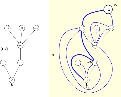
Figure 2: The Cori–Vauquelin–Schaeffer bijection. There are two possible rootings of $\mathbf{q}$: they are indicated with question marks. The maximal geodesic from the corner $c_{0}$ to $v_{*}$ has been magnified.

3.2 Slices

We now follow [26] and describe a modification of the previous construction that, roughly speaking, cuts open the maximal geodesic of $\mathbf{q}$ from $c_{0}$ to $v_{*}$. See Figure 3 for an example, and compare with Figure 2.

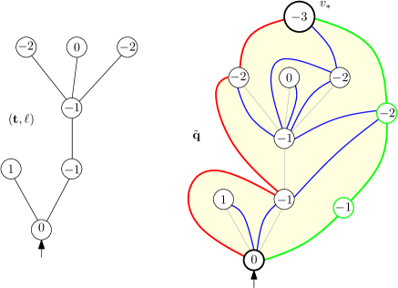
Figure 3: A map with geodesic boundary is associated with a well-labeled tree via the modified Schaeffer bijection. The maximal geodesic is represented in red on the left and the shuttle is the green chain on the right.

Rather than appending to $\mathbf{t}$ a single corner $c_{\infty}$ incident to a vertex $v_{*}$, we add a sequence of corners $c^{\prime}_{1}$, $c^{\prime}_{2}$, …, $c^{\prime}_{\ell(c_{0})-\ell_{*}-1}$, $c^{\prime}_{\ell(c_{0})-\ell_{*}}=c_{\infty}$, and set labels $\ell(c^{\prime}_{i})=\ell(c_{0})-i$, so in particular this is consistent with the label we already set for $c_{\infty}$. Also, instead of extending the sequence $c_{0}$, $c_{1}$, …, $c_{2n-1}$ by periodicity, we add an extra corner $c_{2n}$ to the right of $c_{0}$ and we let $c_{2n+i}=c^{\prime}_{i}$ for $i\in\{1,2,\ldots,\ell(c_{0})-\ell_{*}\}$. The definition of the successor

$$s(i)=\inf\{j>i:\ell(c_{j})=\ell(c_{i})-1\}\,,\qquad s(c_{i})=c_{s(i)}$$ (17)

then makes sense for $i\in\{0,1,\ldots,2n+\ell(c_{0})-\ell_{*}-1\}$, and we can draw the arcs from $c_{i}$ to $s(c_{i})$ for every $i\in\{0,1,\ldots,2n+\ell(c_{0})-\ell_{*}-1\}$. In particular, note that the arcs link $c_{2n}$ with $c^{\prime}_{1}$, $c^{\prime}_{2}$, …, $c^{\prime}_{\ell(c_{0})-\ell_{*}-1}$, $c_{\infty}$ into a chain, which we call shuttle, and to which are connected the arcs $c_{i}\to s(c_{i})$ with $i\leq 2n-1$ and $s(i)>2n-1$. Let $\tilde{\mathbf{q}}$ be the map obtained by this construction. It is called the slice coded by $(\mathbf{t},\ell)$.

This map contains two distinguished geodesic chains, which are, on the one hand, the maximal geodesic from $c_{0}$ to $v_{*}$ made of arcs between consecutive successors $c_{0}$, $s(c_{0})$, $s(s(c_{0}))$, …, $c_{\infty}$ and, on the other hand, the shuttle linking $c_{2n}$, $c^{\prime}_{1}$, $c^{\prime}_{2}$, …, $c^{\prime}_{\ell(c_{0})-\ell_{*}-1}$, $c_{\infty}$. Note that both chains indeed have the same length (number of edges), equal to $\ell(c_{0})-\ell_{*}$. In particular, we have $d_{\tilde{\mathbf{q}}}(c_{0},c_{\infty})=d_{\mathbf{q}}(c_{0},c_{\infty})=\ell(c_{0})-\ell_{*}$, where $\mathbf{q}$ is the quadrangulation from the previous section, constructed from the same well-labeled tree $(\mathbf{t},\ell)$. These two chains are incident to a face of $\tilde{\mathbf{q}}$ of degree $2d_{\mathbf{q}}(c_{0},c_{\infty})$, and all other faces have degree $4$. Observe that the maximal geodesic and the shuttle only intersect at the root vertex of the tree and $v_{*}$; as a result, the boundary of the degree $2d_{\mathbf{q}}(c_{0},c_{\infty})$-face is a simple curve.

Finally, the quadrangulation $\mathbf{q}$ can then be obtained from $\tilde{\mathbf{q}}$ by identifying one by one the edges of the maximal geodesic with the edges of the shuttle, in the same order. More precisely, we note that there is a natural projection $p$ from $E(\tilde{\mathbf{q}})$ to $E(\mathbf{q})$ defined by $p(e)=e$ for every edge $e$ that is not an edge of the shuttle, and $p(e^{\prime}_{i})=e_{i}$ if $e_{i}$ is the $i$-th edge on the maximal geodesic, and $e^{\prime}_{i}$ is the $i$-th edge of the shuttle, starting from $c_{0}$. In particular, $p^{-1}(e)$ contains two edges of $\tilde{\mathbf{q}}$ if and only if $e$ is a vertex of the maximal geodesic of $\mathbf{q}$. The projection $p$ induces also a projection, still denoted by $p$, from $V(\tilde{\mathbf{q}})$ onto $V(\mathbf{q})$ such that, if $u$, $v$ are the extremities of $e$, then $p(u)$, $p(v)$ are the extremities of $p(e)$. For this reason, any path in $\tilde{\mathbf{q}}$ projects into a path in $\mathbf{q}$ via $p$, and the graph distances satisfy the inequality

$$d_{\mathbf{q}}(p(u),p(v))\leq d_{\tilde{\mathbf{q}}}(u,v)\,,\qquad u,v\in V(\tilde{\mathbf{q}})\,.$$

Using the same idea as in the preceding section, we obtain another useful bound for distances in $\tilde{\mathbf{q}}$, as follows. Again, let $v_{i}$ be the vertex incident to the corner $c_{i}$, and $\ell(i)=\ell(v_{i})$. Then

$$d_{\tilde{\mathbf{q}}}(v_{i},v_{j})\leq\ell(i)+\ell(j)-2\check{\ell}(i\wedge j,i\vee j)+2\,,$$ (18)

where $\check{\ell}(i,j)$ is again defined as the minimal value of $\ell$ between $i$ and $j$. Again, this upper bound corresponds to the length of a concatenation of maximal geodesics from $c_{i}$, $c_{j}$ to $v_{*}$ up to the point where they coalesce. In words, the difference is that by taking systematically $\check{\ell}(i\wedge j,i\vee j)$ in the definition rather than the maximum of $\{\check{\ell}(i,j),\check{\ell}(j,i)\}$, we do not allow to “jump” from the shuttle to the maximal geodesic boundary (or vice-versa), which would result in a path present in $\mathbf{q}$ but not in $\tilde{\mathbf{q}}$.

3.3 Plane quadrangulations with a boundary

We now present the variant for plane quadrangulation with a boundary, which is a particular case of the Bouttier–Di Francesco–Guitter bijection [14]. We rather use the presentation of [9], better fitted to our situation.

The encoding object of a plane quadrangulation with a boundary having $n$ internal faces and perimeter $2l$ is a forest $\mathbf{f}=(\mathbf{t}_{1},\dots,\mathbf{t}_{l})$ of $l$ trees with $n$ edges in total, together with a labeling function $\ell:\mathbf{V}(\mathbf{f})=\bigsqcup_{i}\mathbf{V}(\mathbf{t}_{i})\to\mathbb{Z}$ satisfying the following:

• for $1\leq i\leq l$, the tree $\mathbf{t}_{i}$ equipped with the restriction of $\ell$ to $V(\mathbf{t}_{i})$ is a well-labeled tree;

• for $1\leq i\leq l$, we have $\ell(\rho_{i+1})\geq\ell(\rho_{i})-1$, where $\rho_{i}$ denotes the root vertex of $\mathbf{t}_{i}$ and setting $\ell(\rho_{l+1})=\ell(\rho_{1})$ by convention.

Note that the condition on the labels of the root vertices is different from the condition on the labels of neighboring vertices of a given tree. The reader familiar with the Bouttier–Di Francesco–Guitter bijection may recognize the label condition for faces of even degree more than $4$. We will come back to this during Section 6.

Here and later, it will be convenient to normalize $\ell$ by asking that $\ell(\rho_{1})=0$. As before, we define $\ell_{*}=\min\{\ell(v):v\in\mathbf{V}(\mathbf{f})\}-1$. We identify $\mathbf{f}$ with the map obtained by adding $l$ edges linking the roots $\rho_{1}$, $\rho_{2}$, …, $\rho_{l}$ of the successive trees in a cycle. This map has two faces, one of degree $2n+l$ (the bounded one on Figure 4) and one of degree $l$ (the unbounded one on Figure 4). We then follow a procedure similar to that of Section 3.1. We let $c_{0}$, $c_{1}$, …, $c_{2n+l-1}$ be the sequence of corners of the face of degree $2n+l$ in contour order, starting from the root corner of $\mathbf{t}_{1}$. We extend this list by periodicity and add one corner $c_{\infty}$ incident to a vertex $v_{*}$ lying inside the face of degree $2n+l$, with label $\ell(c_{\infty})=\ell(v_{*})=\ell_{*}$. We define the successor functions by (17) and draw an arc from $c_{i}$ to $s(c_{i})$ for every $i\in\{0,1,\ldots,2n+l-1\}$, in such a way that this arc does not cross the edges of $\mathbf{f}$, or other arcs.

The embedded graph $\mathbf{q}$ with vertex set $\mathbf{V}(\mathbf{f})\cup\{v_{*}\}$ and edge set given by the added arcs is a plane quadrangulation with a boundary, whose external face is the degree-$2l$ face corresponding to the face of degree $l$. It is rooted at the corner of the unbounded face that is incident to the root vertex of $\mathbf{t}_{1}$, and it is naturally pointed at $v_{*}$. See Figure 4.

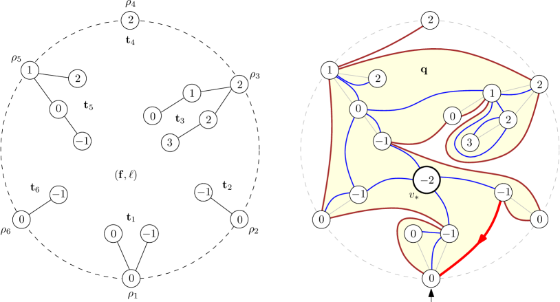
Figure 4: The bijection for a plane quadrangulation with a boundary. The $l$ edges we added to $\mathbf{f}$ are represented by dotted lines and the root edge of $\mathbf{q}$ is represented in red. Note that we used for $\ell$ the normalization given by $\ell(\rho_{1})=0$.

The above mapping is a bijection between previously described labeled forests and the set of pointed plane quadrangulations $(\mathbf{q},v_{*})$ with a boundary having $n$ internal faces and perimeter $2l$ that further satisfy the property that $d_{\mathbf{q}}(e_{*}^{+},v_{*})=d_{\mathbf{q}}(e_{*}^{-},v_{*})+1$, where $e_{*}$ denotes the root edge of $\mathbf{q}$, that is, the oriented edge incident to the root face that directly precedes the root corner in the contour order (see Figure 4). In words, the pointed quadrangulations that are in the image of the above mapping are those whose root edge points away from the distinguished vertex $v_{*}$.

The requirement that the root edge is directed away from the distinguished vertex is not a serious issue, as we can dispose of this constraint simply by re-rooting along the boundary:

Lemma 10.

Let $(Q,v_{*})$ be uniformly distributed in the set ${\bf Q}_{l,n}^{\bullet,+}$ of rooted and pointed quadrangulations such that $Q\in{\bf Q}_{l,n}$ and such that the root edge $e_{*}$ points away from $v_{*}$. Let $c^{\prime}$ be a uniformly chosen random corner incident to the root face of $Q$, and let $Q^{\prime}$ be the map $Q$ re-rooted at $c^{\prime}$. Then $Q^{\prime}$ is a uniform random element of ${\bf Q}_{l,n}$.

Proof.

The probability that $Q^{\prime}$ is a given rooted map $\mathbf{q}^{\prime}$ is equal

$$\mathbb{P}(Q^{\prime}=\mathbf{q}^{\prime})=\frac{1}{2l}\sum_{v\in\mathbf{V}(\mathbf{q}^{\prime})}\sum^{+}_{c}\mathbb{P}((Q,v_{*})=(\mathbf{q},v))=\frac{1}{2l}\sum_{v\in\mathbf{V}(\mathbf{q}^{\prime})}\sum^{+}_{c}\frac{1}{|{\bf Q}_{l,n}^{\bullet,+}|}\,,$$

where the factor $1/2l$ is the probability that $c^{\prime}$ is chosen to be the root corner of $\mathbf{q}^{\prime}$, the symbol $\sum^{+}_{c}$ stands for the sum over all corners incident to the root face of $\mathbf{q}^{\prime}$ that point away from $v$, and $\mathbf{q}$ is the map $\mathbf{q}^{\prime}$ re-rooted at the corner $c$.

Now fix the vertex $v\in\mathbf{V}(\mathbf{q}^{\prime})$. Due to the bipartite nature of $\mathbf{q}^{\prime}$, among the $2l$ oriented edges incident to the root face, $l$ are pointing away from $v$, and $l$ are pointing toward $v$. Indeed, let $\tilde{c}_{0}$ be the root corner of $Q$, and $\tilde{c}_{1}$, $\tilde{c}_{2}$, …, $\tilde{c}_{2l-1}$, $\tilde{c}_{2l}=\tilde{c}_{0}$ be the corners incident to the root face in cyclic order. The sequence $(d_{\mathbf{q}^{\prime}}(\tilde{c}_{i},v_{*}),\,0\leq i\leq 2l)$ takes integer values, varies by $\pm 1$ at every step as $\mathbf{q}^{\prime}$ is bipartite, and takes the same value at times $0$ and $2l$. This means that $l$ of its increments are equal to $+1$ and $l$ are equal to $-1$, respectively corresponding to edges that point away from $v$ and toward $v$.

Therefore, the sum $\sum^{+}_{c}$ contains exactly $l$ elements. Noting that every map in ${\bf Q}_{l,n}$ has $n+l+1$ vertices, by the Euler characteristic formula, this gives

$$\mathbb{P}(Q^{\prime}=\mathbf{q}^{\prime})=\frac{n+l+1}{2\,|{\bf Q}_{l,n}^{\bullet,+}|}\,,$$

which depends only on $n$, $l$ and not on the particular choice of $\mathbf{q}^{\prime}$. ∎

4 Scaling limit of slices

In this section, we elaborate on Proposition 3.3 and Proposition 9.2 in [26], by showing that uniform random slices converge after rescaling to a limiting metric space, which can be called the Brownian map with a geodesic boundary. Such a property was indeed shown in [26], but with a description of the limit that is different from the one we will need.

4.1 Subsequential convergence

Let $(T_{n},\ell_{n})$ be a random variable that is uniformly distributed over the set of well-labeled trees with $n$ edges. With this random variable, we can associate two pointed and rooted random maps $(Q_{n},v_{*})$ and $(\tilde{Q}_{n},v_{*})$ by the constructions of Sections 3.1 and 3.2 respectively. We use the same notation for the distinguished vertex $v_{*}$ since $Q_{n}$ and $\tilde{Q}_{n}$ share naturally the same vertex set, except for the extra vertices on the shuttle of $\tilde{Q}_{n}$.

Let $c_{0}$, $c_{1}$, …, $c_{2n-1}$, $c_{2n}=c_{0}$ be the sequence of corners of $T_{n}$ starting from the root corner, and let $v_{i}$ be the vertex incident to $c_{i}$ in $T_{n}$. We let $C_{n}(i)$ be the distance in $T_{n}$ between the vertices $v_{0}$ and $v_{i}$, so that $C_{n}(i)$ can be seen as the height of $v_{i}$ in the tree $T_{n}$ rooted at $c_{0}$. The process $(C_{n}(i),0\leq i\leq 2n)$, extended to a continuous random function on $[0,2n]$ by linear interpolation between integer values, is called the contour process of $T_{n}$. Similarly, we let $\ell_{n}(i)=\ell_{n}(v_{i})$ and call the process $(\ell_{n}(i),0\leq i\leq 2n)$, which we also extend to $[0,2n]$ in a similar fashion, the label process of $(T_{n},\ell_{n})$.

For $0\leq i,j\leq 2n$, let $D_{n}(i,j)=d_{Q_{n}}(v_{i},v_{j})$ and $\tilde{D}_{n}(i,j)=d_{\tilde{Q}_{n}}(i,j)$. We extend $D_{n}$, $\tilde{D}_{n}$ to continuous functions on $[0,2n]^{2}$ by “bilinear interpolation,” writing $\{s\}=s-\lfloor s\rfloor$ for the fractional part of $s$ and then setting

$$\begin{split}D_{n}(s,t)&=(1-\{s\})(1-\{t\})D_{n}(\lfloor s\rfloor,\lfloor t\rfloor)+\{s\}(1-\{t\})D_{n}(\lfloor s\rfloor+1,\lfloor t\rfloor)\\ &\qquad\qquad+(1-\{s\})\{t\}D_{n}(\lfloor s\rfloor,\lfloor t\rfloor+1)+\{s\}\{t\}D_{n}(\lfloor s\rfloor+1,\lfloor t\rfloor+1),\end{split}$$ (19)

and similarly for $\tilde{D}_{n}$. We define the renormalized versions of $C_{n}$, $\ell_{n}$, $D_{n}$ and $\tilde{D_{n}}$ by

$$C_{(n)}(s)=\frac{C_{n}(2ns)}{\sqrt{2n}}\,,\quad\ell_{(n)}(s)=\left(\frac{9}{8n}\right)^{1/4}\ell_{n}(2ns)\,,$$

and

$$D_{(n)}(s,t)=\left(\frac{9}{8n}\right)^{1/4}D_{n}\big{(}2ns,2nt\big{)}\,,\qquad\tilde{D}_{(n)}(s,t)=\left(\frac{9}{8n}\right)^{1/4}\tilde{D}_{n}\big{(}2ns,2nt\big{)}$$

for every $s$, $t\in[0,1]$.

From [26, Proposition 3.1], it holds that up to extraction, one has the joint convergence

$$(C_{(n)},\ell_{(n)},D_{(n)},\tilde{D}_{(n)})\mathrel{\mathop{\kern 0.0pt\longrightarrow}\limits_{n\to\infty}^{(d)}}(\mathbf{e},Z,D,\tilde{D})\,,$$ (20)

where $\mathbf{e}$ is the normalized Brownian excursion, $Z$ is the head of the snake driven by $\mathbf{e}$ (which is defined as the process $Z^{\mathbf{0}}$ around (12), with $\mathbf{e}$ in place of $X$) and $D$, $\tilde{D}$ are two random pseudo-metrics on $[0,1]$ such that $D\leq\tilde{D}$. In the rest of this section, we are going to fix one extraction along which this convergence holds, and always assume that the values of $n$ that we consider belong to this particular extraction. Moreover, by a use of the Skorokhod representation theorem, we may and will assume that the convergence holds in fact in the a.s. sense.

For $s$, $s^{\prime}\in[0,1]$, define $d_{\mathbf{e}}(s,s^{\prime})=\mathbf{e}_{s}+\mathbf{e}_{s^{\prime}}-2\inf_{s\wedge s^{\prime}\leq u\leq s\vee s^{\prime}}\mathbf{e}_{u}$, $d_{Z}(s,s^{\prime})$ as in formula (14) (with $A=1$), and let

$$\tilde{d}_{Z}(s,s^{\prime})=Z_{s}+Z_{s^{\prime}}-2\underline{Z}_{s\wedge s^{\prime},s\vee s^{\prime}}\,,$$

so that clearly one has $d_{Z}\leq\tilde{d}_{Z}$. The quotient space $S=[0,1]/\{D=0\}$ endowed with the distance induced by $D$ (and still denoted by $D$), is the so-called Brownian map. Likewise, we set $\tilde{S}=[0,1]/\{\tilde{D}=0\}$ and endow it with the induced distance still denoted by $\tilde{D}$. We let $\mathbf{p}:[0,1]\to S$, $\tilde{\mathbf{p}}:[0,1]\to\tilde{S}$ denote the canonical projections, which are continuous since $D$, $\tilde{D}$ are continuous functions on $[0,1]^{2}$. Note that, since $D\leq\tilde{D}$, there exists a unique continuous (even $1$-Lipschitz) projection $\pi:\tilde{S}\to S$ such that $\mathbf{p}=\pi\circ\tilde{\mathbf{p}}$.

The main result of [26, 34] states that a.s., for every $s$, $t\in[0,1]$, $D(s,t)$ is given by the explicit formula

$$D(s,t)=\inf\left\{\sum_{j=1}^{k}d_{Z}(s_{j},t_{j}):\begin{array}[]{l}k\geq 1\,,\quad t_{1},s_{2},t_{2},\ldots,s_{k}\in[0,1],\,s_{1}=s,\,t_{k}=t,\\ d_{\mathbf{e}}(t_{j},s_{j+1})=0\,\mbox{ for every }j\in\{1,\ldots,k-1\}\end{array}\right\}\,.$$ (21)

The main goal of this section is to show that the following analog formula holds for $\tilde{D}$. First, we recall from [26] that $\tilde{D}\leq\tilde{d}_{Z}$ and that $\{d_{\mathbf{e}}=0\}\subseteq\{\tilde{D}=0\}$. Note that the first of these two properties results from a simple passage to the limit in the bound (18). We let $\tilde{D}^{*}$ be the largest pseudo-metric on $[0,1]$ such that these two facts are verified, that is,

$$\tilde{D}^{*}(s,t)=\inf\left\{\sum_{j=1}^{k}\tilde{d}_{Z}(s_{j},t_{j}):\begin{array}[]{l}k\geq 1\,,\quad t_{1},s_{2},t_{2},\ldots,s_{k}\in[0,1],\,s_{1}=s,\,t_{k}=t,\\ d_{\mathbf{e}}(t_{j},s_{j+1})=0\,\mbox{ for every }j\in\{1,\ldots,k-1\}\end{array}\right\}\,.$$

In particular, $\tilde{D}\leq\tilde{D}^{*}$. We will show that $\tilde{D}=\tilde{D}^{*}$ a.s., and in particular, the convergence in (20) holds without having to extract a subsequence. Results by Le Gall [26, Propositions 3.3 and 9.2] provide yet another formula for $\tilde{D}$, which is expressed in terms of cutting the space $(S,D)$ along a certain distinguished geodesic. However, it is not clear that this formula is equivalent to $\tilde{D}=\tilde{D}^{*}$.

Theorem 11.

Almost surely, it holds that for every $s$, $t\in[0,1]$, $\tilde{D}(s,t)=\tilde{D}^{*}(s,t)$.

Moreover, we have for every $x$, $y\in\tilde{S}$,

$$\tilde{D}(x,y)=\inf\left\{\mathrm{length}_{D}(\pi\circ\gamma):\begin{array}[]{c}\gamma:[0,1]\to\tilde{S}\mbox{ continuous}\\ \gamma(0)=x,\gamma(1)=y\end{array}\right\}$$

where $\tilde{S}$ is endowed with the quotient topology of $[0,1]/\{\tilde{D}=0\}$.

Here, the length function is defined as follows. If $(M,d)$ is a metric space (or a pseudo-metric space), and $\gamma:[0,1]\to M$ is a continuous path, we let

$$\mathrm{length}_{d}(\gamma)=\sup\sum_{i=1}^{k}d\big{(}\gamma(r_{i-1}),\gamma(r_{i})\big{)}\,,$$

where the supremum is taken over all partitions $0=r_{0}<r_{1}<\ldots<r_{k-1}<r_{k}=1$ of $[0,1]$.

4.2 Basic properties of the limit spaces

We will need some more properties of the distances $D$, $\tilde{D}$, $\tilde{D}^{*}$. An important fact that we will need is the following identification of the sets $\{D=0\}$, $\{\tilde{D}=0\}$, $\{\tilde{D}^{*}=0\}$, which is a reformulation of [24, Theorem 4.2], [28, Lemma 3.2] and [26, Proposition 3.1] in our setting. Point (12) comes from [29, Proposition 2.5] and [26, Proposition 3.2].

Lemma 12.

(i) Almost surely, for every $s$, $t\in[0,1]$ such that $s\neq t$, it holds that $D(s,t)=0$ if and only if either $d_{\mathbf{e}}(s,t)=0$ or $d_{Z}(s,t)=0$, these two cases being mutually exclusive, with the only exception of $\{s,t\}=\{0,1\}$.

(ii) Likewise, almost surely, for every $s$, $t\in[0,1]$ such that $s\neq t$, it holds that $\tilde{D}(s,t)=0$ if and only if either $d_{\mathbf{e}}(s,t)=0$ or $\tilde{d}_{Z}(s,t)=0$, and these two cases are mutually exclusive.

(iii) There is only one time $s_{*}\in[0,1]$ such that $Z_{s_{*}}=\inf_{[0,1]}Z$. Moreover, $D(0,s_{*})=\tilde{D}(0,s_{*})=-Z_{s_{*}}$.

This implies that the equivalence relations $\{\tilde{D}=0\}$ and $\{\tilde{D}^{*}=0\}$ coincide, since $\tilde{D}\leq\tilde{D}^{*}\leq\tilde{d}_{Z}$ and $\{d_{\mathbf{e}}=0\}\subseteq\{\tilde{D}^{*}=0\}$ by definition. In particular, we see that $\tilde{S}=[0,1]/\{\tilde{D}^{*}=0\}$ endowed with the induced metric $\tilde{D}^{*}$ is homeomorphic to $(\tilde{S},\tilde{D})$.

Note that (12) and (12) in the last statement are very closely related. One sees that the points $s<t$ such that $D(s,t)=0$ but $\tilde{D}(s,t)\neq 0$ are exactly the points such that

$$Z_{s}=\inf_{[0,s]}Z=\inf_{[t,1]}Z=Z_{t}\qquad\text{ and }(s,t)\neq(0,1)\,.$$

Indeed, the previous equalities imply that $d_{Z}(s,t)=0$ and that $\inf_{[s,t]}Z<Z_{s}$, by (12), so that $\tilde{d}_{Z}(s,t)>0$; furthermore, $d_{Z}(s,t)=0$ and $(s,t)\neq(0,1)$ imply by (12) that $d_{\mathbf{e}}(s,t)>0$. This entails that, for $s<t$ of this form, one has that $x=\mathbf{p}(s)=\mathbf{p}(t)\in S$ has two preimages $\pi^{-1}(x)=\{\tilde{\mathbf{p}}(s),\tilde{\mathbf{p}}(t)\}\in\tilde{S}$, while for any other point $x\in S$, $\pi^{-1}(x)$ is a singleton.

More precisely, let $\Delta=D(0,s_{*})=\tilde{D}(0,s_{*})$ and, for $r\in[0,\Delta]$, let

$$\Gamma_{0}(r)=\inf\{s\geq 0:Z_{s}=-r\}\,,\qquad\mbox{ and }\qquad\Gamma_{1}(r)=\sup\{s\geq 0:Z_{s}=-r\}\,.$$

We also let $\gamma_{i}(r)=\tilde{\mathbf{p}}(\Gamma_{i}(r))$ for $i\in\{0,1\}$ and $r\in[0,\Delta]$, and $\gamma(r)=\mathbf{p}(\Gamma_{0}(r))=\mathbf{p}(\Gamma_{1}(r))$. We let $\overset{\circ}{\gamma}_{0}=\gamma_{0}((0,\Delta))$ and we define $\overset{\circ}{\gamma}_{1}$ and $\overset{\circ}{\gamma}$ in a similar fashion.

Corollary 13.

It holds that $\overset{\circ}{\gamma}_{0}\cap\overset{\circ}{\gamma}_{1}=\varnothing$. Moreover, the projection $\pi$ is one-to-one from $\tilde{S}\setminus(\overset{\circ}{\gamma}_{0}\cup\overset{\circ}{\gamma}_{1})$ onto $S\setminus\overset{\circ}{\gamma}$, while $\pi^{-1}(\gamma(r))=\{\gamma_{0}(r),\gamma_{1}(r)\}$ for every $r\in[0,\Delta]$, and the latter is a singleton if and only if $r\in\{0,\Delta\}$.

Next, we say that a metric space $(M,d)$ is a length space if for every $x$, $y\in M$, $d(x,y)=\inf\mathrm{length}_{d}(\gamma)$ where the infimum is taken over all continuous paths $\gamma:[0,1]\to M$ with $\gamma(0)=x$ and $\gamma(1)=y$. A path $\gamma$ for which the infimum is attained is called a geodesic, and a geodesic metric space is a length space $(M,d)$ such that every pair of points is joined by a geodesic. A compact length space is a geodesic space by [17, Theorem 2.5.23].

Lemma 14.

The spaces $(S,D)$, $(\tilde{S},\tilde{D})$ and $(\tilde{S},\tilde{D}^{*})$ are compact geodesic metric spaces.

Proof.

We only sketch the proof of this lemma. Recall that the property of being a compact geodesic metric space is preserved by taking Gromov–Hausdorff limits, by [17, Theorem 7.5.1]. Now, we use the fact that $(S,D)$, $(\tilde{S},\tilde{D})$ are Gromov–Hausdorff limits of the metric spaces $(V(Q_{n}),(9/8n)^{1/4}d_{Q_{n}})$ and $(V(\tilde{Q}_{n}),(9/8n)^{1/4}d_{\tilde{Q}_{n}})$, which in turn are at distance less than $(9/8n)^{1/4}$ from metric graphs obtained by linking any two adjacent vertices by an edge of length $(9/8n)^{1/4}$, the latter being geodesic metric spaces. For $(\tilde{S},\tilde{D}^{*})$, this comes from the fact that $\tilde{D}^{*}$ is a quotient pseudo-metric of the space $([0,1]/\{\tilde{d}_{Z}=0\},\tilde{d}_{Z})$ with respect to the equivalence relation induced on $[0,1]/\{\tilde{d}_{Z}=0\}$ by $\{d_{\mathbf{e}}=0\}$. Since $([0,1]/\{\tilde{d}_{Z}=0\},\tilde{d}_{Z})$ is a length space (it is indeed an $\mathbb{R}$-tree), the quotient pseudo-metric $(\tilde{S},\tilde{D}^{*})$ is also a length space, hence a geodesic space since it is compact. See the discussion after Exercise 3.1.13 in [17]. ∎

We conclude by mentioning that the mappings $r\mapsto\gamma_{0}(r)$ and $r\mapsto\gamma_{1}(r)$ are geodesics in $(\tilde{S},\tilde{D})$ and that $r\mapsto\gamma(r)$ is a geodesic in $(S,D)$. This follows easily from approximations ($\gamma_{0}$ is the continuum counterpart to the maximal geodesic in Section 3.2, and $\gamma_{1}$ to the shuttle) and is discussed in [26].

4.3 Local isometries between $\tilde{S}$ and $S$

In the following, if $(M,d)$ is a metric space or a pseudo-metric space, and if $x\in M$, $A\subseteq M$, we let $d(x,A)=\inf\{d(x,y):y\in A\}$. For $i\in\{0,1\}$, we also use the shorthand $\Gamma_{i}$, $\gamma_{i}$ to designate the image sets $\{\Gamma_{i}(r),0\leq r\leq\Delta\}$ and $\{\gamma_{i}(r),0\leq r\leq\Delta\}$.

Lemma 15.

The following holds almost surely. Fix $\varepsilon>0$, $i\in\{0,1\}$, and let $s$, $t\in[0,1]$ be such that $\tilde{D}(s,\Gamma_{i})\wedge\tilde{D}(t,\Gamma_{i})>\varepsilon$ and $\tilde{D}(s,t)<\varepsilon/2$. Then, it holds that $\tilde{D}(s,t)=D(s,t)=\tilde{D}^{*}(s,t)$.

Proof.

Assume that $i=0$. Let $i_{n}$, $j_{n}\in\{0,1,\ldots,2n\}$ be such that $i_{n}/2n\to s$ and $j_{n}/2n\to t$ as $n\to\infty$. Recall that, throughout this section, we have fixed an extraction along which (20) holds and that $n\to\infty$ is understood along this extraction. Then,

$$\left(\frac{9}{8n}\right)^{1/4}d_{Q_{n}}(v_{i_{n}},v_{j_{n}})\mathrel{\mathop{\kern 0.0pt\longrightarrow}\limits_{n\to\infty}}D(s,t)\,,\qquad\left(\frac{9}{8n}\right)^{1/4}d_{\tilde{Q}_{n}}(v_{i_{n}},v_{j_{n}})\mathrel{\mathop{\kern 0.0pt\longrightarrow}\limits_{n\to\infty}}\tilde{D}(s,t)\,.$$

From the fact that $\tilde{D}(s,\Gamma_{0})>\varepsilon$ we deduce that for every $n$ large enough, the vertex $v_{i_{n}}$ is at $d_{\tilde{Q}_{n}}$-distance at least $(8n/9)^{1/4}\varepsilon$ from the maximal geodesic in $\tilde{Q}_{n}$. Indeed, if this were not the case, then for infinitely many values of $n$, we could find a vertex $v_{k_{n}}$ of the maximal geodesic with $d_{\tilde{Q}_{n}}(v_{k_{n}},v_{i_{n}})\leq(8n/9)^{1/4}\varepsilon$. By definition of the maximal geodesic, it must hold that $\ell_{n}(k_{n})=\inf\{\ell_{n}(i):0\leq i\leq k_{n}\}$, and by passing to the limit up to further extraction, we may assume that $k_{n}/2n$ converges to some $u$ such that $Z_{u}=\inf\{Z_{s},0\leq s\leq u\}$, so that $\tilde{\mathbf{p}}(u)\in\gamma_{0}$ and $\tilde{D}(u,s)\leq\varepsilon$, a contradiction with the fact that $\tilde{D}(s,\Gamma_{0})>\varepsilon$.

Fix $\eta>0$. By (21), there exist $s=s_{1}$, $t_{1}$, …, $s_{k}$, $t_{k}=t$ such that $d_{\mathbf{e}}(t_{m},s_{m+1})=0$ for $1\leq m\leq k-1$, and

$$D(s,t)\geq\sum_{m=1}^{k}d_{Z}(s_{m},t_{m})-\eta\,.$$

Then, we can choose integers $i_{n}(m)$, $j_{n}(m)$, $1\leq m\leq k$ such that $i_{n}(m)/2n\to s_{m}$ and $j_{n}(m)/2n\to t_{m}$ as $n\to\infty$, and we can also require that $v_{j_{n}(m)}=v_{i_{n}(m+1)}$ for all $m\in\{1,\ldots,k-1\}$. Indeed, this last property amounts to the fact that $C_{n}(j_{n}(m))=C_{n}(i_{n}(m+1))$ and that $C_{n}$ is greater than or equal to this common value on $[j_{n}(m)\wedge i_{n}(m+1),j_{n}(m)\vee i_{n}(m+1)]$; we can require this as a simple consequence of the fact that $d_{\mathbf{e}}(t_{m},s_{m+1})=0$ and of the convergence of $C_{(n)}$ to $\mathbf{e}$. For every $m\in\{1,\ldots,k\}$, let $g_{n,m}$ be the maximal wedge path in $Q_{n}$ from $c_{i_{n}(m)}$ to $c_{j_{n}(m)}$, as defined at the end of Section 3.1. The length of this path is given by the upper-bound of (16) for $\ell=\ell_{n}$, $i=i_{n}(m)$ and $j=j_{n}(m)$ and, after renormalization by $(8n/9)^{1/4}$, this length converges to $d_{Z}(s_{m},t_{m})$. Therefore, if we let $g_{n}$ be the concatenation of the paths $g_{n,1}$, $g_{n,2}$, …, $g_{n,k}$, then the length of $g_{n}$ is asymptotically $(8n/9)^{1/4}\sum_{1\leq m\leq k}d_{Z}(s_{m},t_{m})\leq(8n/9)^{1/4}(D(s,t)+\eta)$.

If $g_{n}$ does not intersect the maximal geodesic from the root $c_{0}$ to $v_{*}$ in $Q_{n}$, then $g_{n}$ is also a path in $\tilde{Q}_{n}$ (meaning that it can be lifted via the projection $p$ from $\tilde{Q}_{n}$ to $Q_{n}$, as defined in Section 3.2). In this case, this also means that the maximal wedge paths $g_{n,m}$ are also paths in $\tilde{Q}_{n}$, entailing that their lengths are given by the upper-bounds in (18). If, for infinitely many $n$’s, $g_{n}$ does not intersect the maximal geodesic from the root $c_{0}$ to $v_{*}$ in $Q_{n}$ then, by passing to the limit, we obtain $d_{Z}(s_{m},t_{m})=\tilde{d}_{Z}(s_{m},t_{m})$. We immediately get

$$\tilde{D}(s,t)\leq\tilde{D}^{*}(s,t)\leq\sum_{m=1}^{k}\tilde{d}_{Z}(s_{m},t_{m})=\sum_{m=1}^{k}d_{Z}(s_{m},t_{m})\leq D(s,t)+\eta\,.$$

Since $\eta$ was arbitrary we obtain $\tilde{D}(s,t)\leq\tilde{D}^{*}(s,t)\leq D(s,t)$, but since $D\leq\tilde{D}$, we conclude that this must be an equality all along.

Suppose now that, for infinitely many $n$’s, the path $g_{n}$ does intersect the maximal geodesic from $c_{0}$ to $v_{*}$ in $Q_{n}$. For such an $n$ fixed, let $a$, $b$ be the minimal and maximal integers such that $g_{n}(a)$, $g_{n}(b)$ belong to this path. Clearly, we can modify the path $g_{n}$ by replacing it if necessary by the arc of the maximal geodesic between $g_{n}(a)$ and $g_{n}(b)$ without increasing its length. Now, the vertices $g_{n}(0),g_{n}(1),\ldots,g_{n}(a-1)$ are vertices of $Q_{n}$ that are not in the maximal geodesic, so they lift via the projection $p$ to a path in $\tilde{Q}_{n}$, with same length. The edge between $g_{n}(a-1)$ and $g_{n}(a)$ also lifts into an edge of $\tilde{Q}_{n}$, and it arrives at a point $g^{\prime}_{n}(a)\in p^{-1}(g_{n}(a))$ which is either on the maximal geodesic or on the shuttle of $\tilde{Q}_{n}$. However, the first case is impossible for large $n$’s, since the maximal geodesic is at $d_{\tilde{Q}_{n}}$-distance at least $(8n/9)^{1/4}\varepsilon$ from $v_{i_{n}}=g_{n}(0)$ and $d_{\tilde{Q}_{n}}(g_{n}(0),g^{\prime}_{n}(a))\leq d_{\tilde{Q}_{n}}(v_{i_{n}},v_{j_{n}})\leq(8n/9)^{1/4}\varepsilon/2$. The same argument applies to the path $g_{n}(b)$, $g_{n}(b+1)$, …, $v_{j_{n}}$, which can be viewed as a path in $\tilde{Q}_{n}$ leaving the vertex $g^{\prime}_{n}(b)$ of the shuttle and going to $v_{j_{n}}$. Moreover, since the shuttle projects to a geodesic path in $Q_{n}$, the length $b-a$ of $g_{n}(a)$, $g_{n}(a+1)$, …, $g_{n}(b-1)$, $g_{n}(b)$ is not smaller than the length of the segment of the shuttle between the vertices $g_{n}^{\prime}(a)$ and $g_{n}^{\prime}(b)$.

Therefore, we see that, if $g_{n}$ intersects the maximal geodesic from $c_{0}$ to $v_{*}$ in $Q_{n}$, we can construct from it a path in $\tilde{Q}_{n}$ with same length, going from $v_{i_{n}}$ to $g^{\prime}_{n}(a)$, then taking the segment of the shuttle from $g^{\prime}_{n}(a)$ to $g^{\prime}_{n}(b)$, then going from $g^{\prime}_{n}(b)$ to $v_{j_{n}}$. This path is still a concatenation of maximal wedge paths that are now in $\tilde{Q}_{n}$, so by a new passage to the limit (possibly up to a new extraction), we can find $k^{\prime}\leq k$ and $s=s^{\prime}_{1}$, $t^{\prime}_{1}$, …, $s^{\prime}_{k^{\prime}}$, $t^{\prime}_{k^{\prime}}=t$ such that, for every $m$,

$$\tilde{d}_{Z}(s^{\prime}_{m},t^{\prime}_{m})=d_{Z}(s^{\prime}_{m},t^{\prime}_{m})\,,\qquad d_{\mathbf{e}}(t^{\prime}_{m},s^{\prime}_{m+1})=0\,,$$

and such that

$$D(s,t)+\eta\geq\sum_{m=1}^{k}d_{Z}(s_{m},t_{m})\geq\sum_{m=1}^{k^{\prime}}d_{Z}(s^{\prime}_{m},t^{\prime}_{m})=\sum_{m=1}^{k^{\prime}}\tilde{d}_{Z}(s^{\prime}_{m},t^{\prime}_{m})\geq\tilde{D}^{*}(s,t)\geq\tilde{D}(s,t)\,.$$

Again, since $\eta$ was arbitrary, this yields $D(s,t)=\tilde{D}^{*}(s,t)=\tilde{D}(s,t)$.

We obtain the same result with $\Gamma_{1}$ replaced by $\Gamma_{0}$ by a similar reasoning. ∎

4.4 Proof of Theorem 11

We now turn the “local” lemma that we just proved into a “global” result, which is the content of Theorem 11.

Proof of Theorem 11.

Fix two points $x$, $y\in\tilde{S}$, and a continuous, injective path $f:[0,1]\to\tilde{S}$ going from $x$ to $y$.

For every $r\in[0,1]$, let $F(r)\in[0,1]$ be an arbitrary point such that $\tilde{\mathbf{p}}(F(r))=f(r)$. Suppose first that $f$ does not visit the points $\tilde{\mathbf{p}}(0)$ and $\tilde{\mathbf{p}}(s_{*})$. Then for every $r\in[0,1]$, $\tilde{\mathbf{p}}(F(r))$ is either not in $\gamma_{0}$, or not in $\gamma_{1}$. Assume for the moment that we are in the first case. It means that we can find a neighborhood $V_{r}$ of $r$ in $[0,1]$ and $\varepsilon_{r}>0$ such that $\tilde{D}(F(r^{\prime}),F(r))<\varepsilon_{r}/2$ and $\tilde{D}(F(r^{\prime}),\Gamma_{0})>\varepsilon_{r}$ for every $r^{\prime}\in V_{r}$. In the second case, a similar property holds with $\Gamma_{1}$ instead of $\Gamma_{0}$. By taking a finite subcover, and applying Lemma 15, we obtain the existence of $\varepsilon>0$ depending on $f$ such that for every $r$, $r^{\prime}\in[0,1]$, $|r-r^{\prime}|\leq\varepsilon$ implies

$$\tilde{D}\big{(}F(r),F(r^{\prime})\big{)}=\tilde{D}^{*}\big{(}F(r),F(r^{\prime})\big{)}=D\big{(}F(r),F(r^{\prime})\big{)}\,.$$

Hence, for every partition $0=r_{0}<r_{1}<\ldots<r_{k}=1$ such that $|r_{i+1}-r_{i}|<\varepsilon$ for every $i\in\{0,\ldots,k-1\}$,

$$\sum_{i=0}^{k-1}\tilde{D}\big{(}F(r_{i}),F(r_{i+1})\big{)}=\sum_{i=0}^{k-1}\tilde{D}^{*}\big{(}F(r_{i}),F(r_{i+1})\big{)}=\sum_{i=0}^{k-1}D\big{(}F(r_{i}),F(r_{i+1})\big{)}\,,$$

which implies that

$$\mathrm{length}_{\tilde{D}}(f)=\mathrm{length}_{\tilde{D}^{*}}(f)=\mathrm{length}_{D}(\pi\circ f)\,.$$ (22)

We now use the easy fact that for any metric space $(M,d)$ and every continuous path $\gamma:[0,1]\to M$, the function $r\mapsto\mathrm{length}_{d}(\gamma|_{[0,r]})$ is a non-decreasing, left-continuous function from $[0,1]$ to $[0,\infty]$. Moreover, the length function is additive in the sense that $\mathrm{length}_{d}(\gamma)=\mathrm{length}_{d}(\gamma|_{[0,r]})+\mathrm{length}_{d}(\gamma|_{[r,1]})$ for every $r\in[0,1]$. These two properties together clearly imply that (22) is still valid if the injective, continuous path $f$ is allowed to visit $\tilde{\mathbf{p}}(0)$, $\tilde{\mathbf{p}}(s_{*})$, or both. Taking the infimum over all such functions from a point $x$ to $y$, and using Lemma 14, we finally get $\tilde{D}(x,y)=\tilde{D}^{*}(x,y)$, and that this quantity is the infimum of $\mathrm{length}_{D}(\pi\circ f)$ over all injective continuous paths from $x$ to $y$ in $\tilde{S}$, hence over all continuous paths from $x$ to $y$ in $\tilde{S}$, not necessarily injective. ∎

5 Proof of Theorem 1

5.1 Subsequential convergence

We now move to quadrangulations with boundaries, which are our main object of interest. Recall the construction of Section 3.3 and consider an encoding labeled forest $(\mathbf{f},\ell)$ for a quadrangulation with a boundary. As in the preceding section, we will further encode it by a pair of real-valued functions. Before we proceed, it will be convenient to add an extra vertex-tree $\rho_{l+1}$ with label $\ell(\rho_{l+1})=\ell(\rho_{1})$ to the forest. This extra vertex does not really play a part but its introduction will make the presentation simpler. We also add $l$ edges between $\rho_{i}$ and $\rho_{i+1}$, for $1\leq i\leq l$. See Figure 5.

We let $c_{0}$, $c_{1}$, …, $c_{2n+l-1}$ be as in Section 3.3 and we add to this list the corner $c_{2n+l}$ incident to the extra vertex-tree $\rho_{l+1}$. We define the contour and label processes on $[0,2n+l]$ by

$$C(j)=d_{\mathbf{f}}(c_{j},\rho_{l+1})-l\quad\text{ and }\quad\ell(j)=\ell(c_{j}),\qquad 0\leq j\leq 2n+l$$

and by linear interpolation between integer values.

Figure 5: The contour and label processes associated with the labeled forest of Figure 4. The extra vertex-tree $\rho_{7}$ and the edges linking the roots are represented with a dashed line. Note that the normalization we chose for the labels is equivalent to imposing $\ell(0)=0$.

Let us fix $L\in(0,\infty)$ and a sequence $(l_{n},n\geq 1)$ such that $l_{n}\sim L\sqrt{2n}$ as $n\to\infty$. We let $(F_{n},\ell_{n})$ be uniformly distributed over the set of labeled forests of $l_{n}$ trees with $n$ edges in total, and let $(Q_{n},v_{*})$ be the random pointed quadrangulation associated with $F_{n}$ via the bijection of Section 3.3. Note that up to re-rooting $Q_{n}$ at a uniform corner incident to the root face, we may assume that $Q_{n}$ is uniform in ${\bf Q}_{l_{n},n}$ by Lemma 10.

We let $C_{n}$, $\ell_{n}$ be the associated contour and label processes, and we define their renormalized versions

$$C_{(n)}(s)=\frac{C_{n}\big{(}(2n+{l_{n}})s\big{)}}{\sqrt{2n}}\,,\qquad\ell_{(n)}(s)=\left(\frac{9}{8n}\right)^{1/4}\ell_{n}\big{(}(2n+{l_{n}})s\big{)}\,,\qquad 0\leq s\leq 1\,.$$

We let $D_{n}(i,j)$ be the distance in $Q_{n}$ between the vertices incident to the $i$-th and $j$-th corner of $F_{n}$, for $i,j\in\{0,1,\ldots,2n+{l_{n}}\}$. We extend $D_{n}$ to a continuous function on $[0,2n+{l_{n}}]^{2}$ by the exact same formula as (19), and we finally define its renormalized version

$$D_{(n)}(s,t)=\left(\frac{9}{8n}\right)^{1/4}D_{n}\big{(}(2n+{l_{n}})\,s,(2n+{l_{n}})\,t\big{)}\,,\qquad 0\leq s,t\leq 1\,.$$ (23)

It is shown in [10] that, from every increasing family of positive numbers, one can extract a further subsequence along which

$$(C_{(n)},\ell_{(n)},D_{(n)})\mathrel{\mathop{\kern 0.0pt\longrightarrow}\limits_{n\to\infty}^{(d)}}(X,Z,D)$$

in distribution in the space $\mathcal{C}([0,1])\times\mathcal{C}([0,1])\times\mathcal{C}([0,1]^{2})$. (At this moment, the need of extracting a subsequence is caused by the last coordinate $D_{(n)}$ and the convergence without extraction holds if one drops this coordinate.) Here, $D$ is a random pseudo-metric on $[0,1]$ and $(X,Z)$ law $\mathbb{F}^{1}_{L}$ defined in Section 2, so that $X$ is a first-passage bridge, attaining level $-L$ for the first time at time $1$, and $Z$ is the associated snake process.

Moreover, the pointed random metric space $(\mathbf{V}(Q_{n}),(9/8n)^{1/4}d_{Q_{n}},v_{*})$ converges in distribution, still along the same subsequence, to the random metric space $([0,1]/\{D=0\},D,x_{*})$, in the sense of the pointed Gromov–Hausdorff topology. Here, we let $x_{*}=\mathbf{p}(s_{*})$, where $\mathbf{p}:[0,1]\to[0,1]/\{D=0\}$ is the canonical projection, and $s_{*}$ is the (a.s. unique [10, Lemma 11]) point in $[0,1]$ at which $Z$ reaches its global minimum.

Proposition 16 ([10]).

Almost surely, the space $\mathbf{D}=[0,1]/\{D=0\}$ is a topological disk whose boundary $\partial\mathbf{D}$ satisfies

$$\mathbf{p}^{-1}(\partial\mathbf{D})=\{s\in[0,1]:X_{s}=\underline{X}_{s}\}\,.$$ (24)

Almost surely, the Hausdorff dimension of $\mathbf{D}$ is 4, and that of $\partial\mathbf{D}$ is $2$.

Recall that $v_{*}$ is a uniform random vertex in $Q_{n}$, conditionally given the latter. From this observation, we obtain an invariance under re-rooting property of $(\mathbf{D},D,x_{*})$, along the same lines as [25].

Lemma 17.

Let $U$ be a uniform random variable in $[0,1]$, independent of $(X,Z,D)$. Then the two pointed spaces $(\mathbf{D},D,\mathbf{p}(U))$ and $(\mathbf{D},D,x_{*})$ have the same distribution.

The following lemma is an easy consequence of the study of geodesics done in [9].

Lemma 18.

Almost surely, for every $x\in\mathbf{D}\setminus\partial\mathbf{D}$, there exists a geodesic from $x$ to $x_{*}$ that does not intersect $\partial\mathbf{D}$. Moreover, this is the only geodesic from $x$ to $x_{*}$ for $\mu$-almost every $x\in\mathbf{D}$, where $\mu=\mathbf{p}_{*}(\mathrm{Leb}_{[0,1]})$.

Proof.

For $s\in[0,1]$, we define the path $\Phi_{s}:[0,D(s_{*},s)]\to\mathbf{D}$ by

$$\Phi_{s}(w)=\mathbf{p}\left(\sup\left\{r\,:\,\underline{Z}_{r,s}=Z_{s_{*}}+w\right\}\right),\qquad 0\leq w\leq D(s_{*},s)=Z_{s}-Z_{s_{*}}.$$

It is shown in [9, Proposition 23] that the path $\Phi_{s}$ is a geodesic from $x_{*}$ to $\mathbf{p}(s)$ in $\mathbf{D}$ and that a.s. all the geodesics from $x_{*}$ are of this form. We call increase point of a function a point $t$ such that the function is greater than its value at $t$ on a small interval of the form $[t-\varepsilon,t]$ or $[t,t+\varepsilon]$ for some $\varepsilon>0$. Clearly, for $0\leq w<D(s_{*},s)$, the point $\sup\left\{r\,:\,\underline{Z}_{r,s}=Z_{s_{*}}+w\right\}$ is an increase point of the process $Z$, which is furthermore different from $0$. On the other hand, the expression (24) shows that $\mathbf{p}^{-1}(\partial\mathbf{D})$ is made only of increase points of $X$, together with the point $0$. Moreover, [9, Lemma 18] states that, a.s., the processes $X$ and $Z$ do not share any increase points. As a consequence, $\Phi_{s}$ may only intersect $\partial\mathbf{D}$ at its endpoint $\mathbf{p}(s)$ and the first statement follows.

In addition, [9, Proposition 17] entails that, for $0\leq s\leq t\leq 1$, $D(s,t)=0$ if and only if one of the following occurs:

1. $X_{s}=X_{t}=\underline{X}_{s,t}$;

2. $Z_{s}=Z_{t}=\underline{Z}_{s,t}$ or $Z_{s}=Z_{t}=\underline{Z}_{t,s}$.

Moreover, for $s\neq t$, only one of the previous situations can happen. In some sense, this can be thought of as a continuous version of the bijection from Section 3.3: point (5.1a) constructs the continuous random forest and drawing an arc between a corner and its successor becomes, in the limit, identifying points with the same label and such that the labels visited in between in the contour order are all larger (point (5.1b)). Standard properties of the process $Z$ then allow us to conclude that $\mathrm{Leb}_{[0,1]}(\{s:\,\exists t\neq s:\,D(s,t)=0\})=0$, so that, for $\mu$-almost every $x\in\mathbf{D}$, the set $\mathbf{p}^{-1}(x)$ is a singleton and the only geodesic from $x_{*}$ to $x$ is thus $\Phi_{\mathbf{p}^{-1}(x)}$. ∎

Combining Lemmas 17 and 18, we see that the conclusion of the latter is still valid if $x_{*}$ is replaced by a uniformly chosen point in $\mathbf{D}$, that is, a random point of the form $\mathbf{p}(U)$ as in the first lemma. Finally, we will use the following result.

Lemma 19 ([10]).

The following properties hold almost surely.

• $D\in\mathcal{D}$.

• $D(s,s_{*})=Z_{s}-Z_{s_{*}}$ for every $s\in[0,1]$.

5.2 Identification of the limit

Recall the notation $D^{*}$ from Section 2.3. In this section, we show the following analog to the first part of Theorem 11.

Theorem 20.

Almost surely, it holds that $D=D^{*}$.

Theorem 1 is an immediate consequence of this. Indeed, since $D^{*}$ is a measurable function of $(X,Z)$, this shows that $D^{*}$ is the only possible subsequential limit of $D_{(n)}$. This, combined with the tightness of the sequence $(D_{(n)},n\geq 1)$ that we alluded to above, implies that $D_{(n)}$ converges in distribution to $D^{*}$.

In turn, this convergence implies that of $(9/8n)^{1/4}Q_{n}$ to $\mathrm{BD}_{L}=(\mathbf{D},D^{*})$ in the Gromov–Hausdorff sense and even that of the pointed space $((9/8n)^{1/4}Q_{n},v_{*})$ to $(\mathrm{BD}_{L},x_{*})$, where we recall that $x_{*}=\mathbf{p}(s_{*})$. Let us recall how to prove this fact. First, one can assume that the convergence of $(C_{(n)},\ell_{(n)},D_{(n)})$ to $(X,Z,D^{*})$ is almost-sure, by using Skorokhod’s representation theorem. Then we define a correspondence $\mathcal{R}_{n}$ between $Q_{n}$ and $\mathrm{BD}_{L}$ by

$$\mathcal{R}_{n}=\{(v_{\lfloor(2n+l_{n})s\rfloor},\mathbf{p}(s)):s\in[0,1]\}\cup\{(v_{*},\mathbf{p}(s_{*}))\}\,,$$

where $v_{i}$ is the vertex of $Q_{n}$ incident to the $i$-th corner $c_{i}$. It is elementary to see from the uniform convergence of $D_{(n)}$ to $D^{*}$ that the distortion of $\mathcal{R}_{n}$ with respect to the metrics $(9/8n)^{1/4}d_{Q_{n}}$ and $D^{*}$ converges to $0$ as $n\to\infty$.

Recall that $[a,b]$ is an excursion interval of $X$ above $\underline{X}$ if $a<b$ and $X_{a}=X_{b}=\underline{X}_{b}$. Let us arrange the excursion intervals of $X$ above $\underline{X}$ as $[a_{i},b_{i}]$, $i\geq 1$ in decreasing order of length. For a given $i$, the excursion interval $[a_{i},b_{i}]$ encodes a slice in the sense of Section 4. Namely, for $s$, $t\in[a_{i},b_{i}]$, let $d_{Z}^{i}(s,t)=Z_{s}+Z_{t}-2\underline{Z}_{s\wedge t,s\vee t}$, and

$$\tilde{D}^{i}(s,t)=\inf\left\{\sum_{j=1}^{k}d^{i}_{Z}(s_{j},t_{j}):\begin{array}[]{l}k\geq 1\,,\quad t_{1},s_{2},t_{2},\ldots,s_{k}\in[a_{i},b_{i}],\,s_{1}=s,\,t_{k}=t,\\ d_{X}(t_{j},s_{j+1})=0\,\mbox{ for every }j\in\{1,\ldots,k-1\}\end{array}\right\}\,.$$

By simple scaling properties and excursion theory, conditionally given the excursion lengths $(b_{i}-a_{i})$, $i\geq 1$, the spaces $\tilde{S}^{i}=[a_{i},b_{i}]/\{\tilde{D}^{i}=0\}$, equipped with the induced distance, still called $\tilde{D}^{i}$, are independent versions of the Brownian slices of Section 4, with distances rescaled by $(b_{i}-a_{i})^{1/4}$ respectively. The next key lemma states that the distance $D$ can be identified as a metric gluing of these slices along their boundaries. This guides the intuition of its proof, which will partly consist in going back to the discrete slices that compose the quadrangulations with a boundary of which we took the limit.

Lemma 21.

Let $\tilde{D}$ be the pseudo-metric on $\bigcup_{i\geq 1}[a_{i},b_{i}]$ defined by $\tilde{D}(s,t)=\tilde{D}^{i}(s,t)$ if $s$, $t\in[a_{i},b_{i}]$ for some $i\geq 1$, and $\tilde{D}(s,t)=\infty$ otherwise. Then for almost every $(s,t)\in[0,1]^{2}$ with respect to the Lebesgue measure, it holds that

$$D(s,t)=\inf\left\{\sum_{j=1}^{k}\tilde{D}(s_{j},t_{j}):\begin{array}[]{l}k\geq 1\,,\quad t_{1},s_{2},t_{2},\ldots,s_{k}\in[0,1],\,s_{1}=s,\,t_{k}=t,\\ d_{Z}(t_{j},s_{j+1})=0\,\mbox{ for every }j\in\{1,\ldots,k-1\}\end{array}\right\}\,.$$

Moreover, the above infimum is attained.

Proof.

Clearly, $D(s,t)\leq d_{Z}(s,t)\leq d_{Z}^{i}(s,t)$ whenever $s$, $t\in[a_{i},b_{i}]$, so that $D(s,t)\leq\tilde{D}(s,t)$ for $s$, $t\in[0,1]$ and, as a consequence, the left-hand side is smaller than the right-hand side. We then only need to prove the converse inequality.

Let us first define the discrete analogs to the functions $\tilde{D}^{i}$. We consider the $i$-th largest tree $\mathbf{t}$ of $F_{n}$ and we suppose that it is visited between times $a_{i}^{n}$ and $b_{i}^{n}$ in the contour order of $F_{n}$. For $j$, $k\in\{a_{i}^{n},\ldots,b_{i}^{n}\}$, we let $\tilde{D}_{n}(j,k)$ be the distance in the slice corresponding to $\mathbf{t}$ between the vertices $v_{j}$ and $v_{k}$ incident to the $j$-th and $k$-th corner of $F_{n}$. In other words, $\tilde{D}_{n}(j,k)$ is the length of a shortest path linking $v_{j}$ to $v_{k}$ and that do not “traverse” the images in $Q_{n}$ of the maximal geodesic and shuttle of the aforementioned slice. We then extend $\tilde{D}_{n}$ to a continuous function on $[a_{i}^{n},b_{i}^{n}]^{2}$ by bilinear interpolation, and define its renormalized version $\tilde{D}^{i}_{(n)}$ on a subsquare of $[0,1]^{2}$ by the analog of (23). We define $\tilde{D}^{i}_{(n)}$ arbitrarily for $i>l_{n}$.

As a simple consequence of the convergence (20), reformulated in the context of the excursion intervals $[a_{i}^{n},b_{i}^{n}]$, and of Theorem 11, we have that

$$\left(C_{(n)},\ell_{(n)},\big{(}\tilde{D}^{i}_{(n)}\big{)}_{i\geq 1}\right)\xrightarrow[n\to\infty]{}\left(X,Z,\big{(}\tilde{D}^{i}\big{)}_{i\geq 1}\right)$$ (26)

in distribution in the space $\mathcal{C}([0,1])\times\mathcal{C}([0,1])\times\mathcal{C}([0,1]^{2})^{N}$. Applying Skorokhod’s representation theorem, we also assume from now on that this convergence holds a.s.

It suffices to prove the claimed formula for $D(s,t)$ when $s$, $t$ are replaced by two independent uniform random variables $U$, $V$, independent of the other random variables considered so far. Let $\gamma:[0,D(U,V)]\to\mathbf{D}$ be the geodesic in $(\mathbf{D},D)$ from $\mathbf{p}(U)$ to $\mathbf{p}(V)$, which by Lemmas 17 and 18 is unique and does not intersect $\partial\mathbf{D}$, a.s. Let also $\mathrm{Im}(\gamma)=\gamma([0,D(U,V)])$ be the image of $\gamma$ and define

$$I(U,V)=\big{\{}i\geq 1:\mathbf{p}^{-1}(\mathrm{Im}(\gamma))\cap[a_{i},b_{i}]\neq\varnothing\big{\}}.$$

Claim 1.

The set $I(U,V)$ is finite almost surely.

Proof.

Let us argue by contradiction, assuming that $I(U,V)$ is infinite with positive probability. Then it holds that, still with positive probability, there is an increasing integer sequence $(i_{n})_{n\geq 1}$ and a sequence $(r_{n})_{n\geq 1}$ with values in $[0,D(U,V)]$ such that $\gamma(r_{n})\in\mathbf{p}([a_{i_{n}},b_{i_{n}}])$. Then, up to extraction, the sequence $(r_{n})$ converges to some limit $r$, and if $s_{n}\in[a_{i_{n}},b_{i_{n}}]$ is a choice of a given element in $\mathbf{p}^{-1}(\gamma(r_{n}))$, then, again up to possibly further extraction, $(s_{n})$ converges to a limit $s$ with $\mathbf{p}(s)=\gamma(r)$. By construction, $s$ is not in $\bigcup_{i\geq 1}(a_{i},b_{i})$, since the intervals in this union are pairwise disjoint. This implies that $X_{s}=\underline{X}_{s}$, meaning that $\gamma(r)=\mathbf{p}(s)\in\partial\mathbf{D}$, which is the contradiction we were looking for. ∎

Let $\gamma^{i}_{l}$, $\gamma^{i}_{r}$ be the left and right “geodesic boundaries” of the space $([a_{i},b_{i}]/d_{Z}^{i},d_{Z}^{i})$, defined by

$$\gamma^{i}_{l}(t)=\mathbf{p}\big{(}\inf\{s\in[a_{i},b_{i}]:Z_{s}=Z_{a_{i}}-t\}\big{)}\,,\quad\gamma^{i}_{r}(t)=\mathbf{p}\big{(}\sup\{s\in[a_{i},b_{i}]:Z_{s}=Z_{a_{i}}-t\}\big{)}\,,$$

where $t$ ranges over $[0,Z_{a_{i}}-\underline{Z}_{a_{i},b_{i}}]$ (recall that $Z_{a_{i}}=Z_{b_{i}}$). Those are geodesic paths in $(\mathbf{D},D)$ from $\mathbf{p}(a_{i})$ to $\mathbf{p}(s_{i}^{*})$, where $s_{i}^{*}$ is the (a.s. unique [29]) time in $[a_{i},b_{i}]$ at which $Z$ attains its infimum on that same interval. Alternatively, these paths are parts of the geodesics $\Phi_{a_{i}}$ and $\Phi_{b_{i}}$ introduced earlier. Note also that $\mathrm{Im}(\gamma^{i}_{l})\cap\mathrm{Im}(\gamma^{i}_{r})$ is not necessarily reduced to $\{\mathbf{p}(s_{i}^{*})\}$.

Claim 2.

It is not possible to find $r_{1}<r_{2}<r_{3}$ such that $\gamma(r_{1}),\gamma(r_{3})\in\mathrm{Im}(\gamma^{i}_{l})$ and $\gamma(r_{2})\notin\mathrm{Im}(\gamma^{i}_{l})$. The same statement is valid for $\gamma^{i}_{r}$ instead of $\gamma^{i}_{l}$.

Proof.

Indeed, such a situation would clearly violate the uniqueness of the geodesic $\gamma$, since we could replace it between times $r_{1}$ and $r_{3}$ by the arc of $\gamma^{i}_{l}$ from $\gamma(r_{1})$ to $\gamma(r_{3})$, and still obtain a geodesic from $\mathbf{p}(U)$ to $\mathbf{p}(V)$, distinct from $\gamma$. ∎

Claim 3.

Almost surely, for every $i\geq 1$, the topological boundary of $\mathbf{p}([a_{i},b_{i}])$ in $(\mathbf{D},D)$ is included in $\mathrm{Im}(\gamma_{l}^{i})\cup\mathrm{Im}(\gamma^{i}_{r})$.

Proof.

This claim is relatively obvious with the interpretation that $([a_{i},b_{i}]/\{\tilde{D}^{i}=0\},\tilde{D}^{i})$ is a space with geodesic boundaries given by $\gamma_{l}^{i}$, $\gamma_{r}^{i}$, but since we are not referring explicitly to these spaces, let us give a complete proof for this. In fact, the topological boundary of $\mathbf{p}([s,t])$ for any $a_{i}\leq s\leq t\leq b_{i}$ is given by [9, Lemma 21] but, as the proof is quite short, we restate the arguments here. Note that $\mathbf{p}([a_{i},b_{i}])$ is closed so that every point in $\partial\mathbf{p}([a_{i},b_{i}])$ is of the form $\mathbf{p}(s^{\prime})$ for some $s^{\prime}\in[a_{i},b_{i}]$ and is a limit of a sequence of points of the form $\mathbf{p}(s_{n})$, $n\geq 1$, where $s_{n}\notin[a_{i},b_{i}]$ for every $n\geq 1$. Up to extraction, $(s_{n})$ converges to a limit $s\notin(a_{i},b_{i})$ such that $D(s,s^{\prime})=0$. If $s\in\{a_{i},b_{i}\}$ then the claim follows immediately. Otherwise, $s\neq s^{\prime}$ and, as mentioned during the proof of Lemma 18, this implies $d_{X}(s,s^{\prime})=0$ (5.1a) or $d_{Z}(s,s^{\prime})=0$ (5.1b). It cannot hold that $d_{X}(s,s^{\prime})=0$ because $s^{\prime}\in[a_{i},b_{i}]$ while $s\notin[a_{i},b_{i}]$, so necessarily $d_{Z}(s,s^{\prime})=0$. Assuming for instance that $Z_{s}=Z_{s^{\prime}}=\underline{Z}_{s,s^{\prime}}$, so that $Z_{u}\geq Z_{s^{\prime}}$ for every $u\in[a_{i},s^{\prime}]$, this implies that $d_{Z}(s,\inf\{u\in[a_{i},b_{i}]:Z_{u}=Z_{s})=0$. Finally, we get that $\mathbf{p}(s)=\gamma_{l}^{i}(Z_{a_{i}}-Z_{s})\in\mathrm{Im}(\gamma^{i}_{l})$. Similarly, if $Z_{s}=Z_{s^{\prime}}=\underline{Z}_{s^{\prime},s}$, we obtain that $\mathbf{p}(s)\in\mathrm{Im}(\gamma^{i}_{r})$. ∎

From the three claims above, we obtain that there exists a finite number of points $x_{1}$, $x_{2}$, …, $x_{k+1}\in\mathbf{D}$ and integers $i_{1}$, …, $i_{k}$ with $x_{1}=\mathbf{p}(U)$, $x_{k+1}=\mathbf{p}(V)$, such that $\gamma$ visits the points $x_{1}$, $x_{2}$, …, $x_{k+1}$ in this order, and such that the segment of $\gamma$ between $x_{j}$ and $x_{j+1}$ is

1. either included in $\mathrm{Im}(\gamma^{i_{j}}_{l})$ or included in $\mathrm{Im}(\gamma^{i_{j}}_{r})$

2. or included in $\mathbf{p}([a_{i_{j}},b_{i_{j}}])$ and such that its intersection with $\mathrm{Im}(\gamma^{i_{j}}_{l})\cup\mathrm{Im}(\gamma^{i_{j}}_{r})$ is a subset of $\{x_{j},x_{j+1}\}$.

Indeed, Claims 1 and 2 entail that $\mathrm{Im}(\gamma)\cap(\bigcup_{i}\mathrm{Im}(\gamma^{i}_{l})\cup\mathrm{Im}(\gamma^{i}_{r}))$ is a finite union of segments satisfying (3a) and the parts of $\gamma$ linking two successive such segments satisfy (3b), by Claim 3. Since the segment of $\gamma$ between $x_{j}$ and $x_{j+1}$ is included in $\mathbf{p}([a_{i_{j}},b_{i_{j}}])$ in both cases, we may choose $s_{j}$, $t_{j}\in[a_{i_{j}},b_{i_{j}}]$ such that $x_{j}=\mathbf{p}(s_{j})$ and $x_{j+1}=\mathbf{p}(t_{j})$. For any such choice,

$$D(U,V)=\sum_{j=1}^{k}D(s_{j},t_{j})\,.$$

We will soon justify that we can choose $s_{j}$, $t_{j}$ satisfying the extra property that $D(s_{j},t_{j})=\tilde{D}(s_{j},t_{j})$ on the event $\{\max(I(U,V))\leq N\}$. Since, by definition, $\mathbf{p}(t_{j})=\mathbf{p}(s_{j+1})$, one has $d_{X}(t_{j},s_{j+1})=0$ or $d_{Z}(t_{j},s_{j+1})=0$ so that $\tilde{D}(t_{j},s_{j+1})=0$ or $d_{Z}(t_{j},s_{j+1})\allowbreak=0$. Similarly, $\tilde{D}(U,s_{1})=0$ or $d_{Z}(U,s_{1})=0$ and $\tilde{D}(t_{k},V)=0$ or $d_{Z}(t_{k},V)=0$. As a result, up to potentially doubling some $s_{j}$’s and $t_{j}$’s, we wrote $D(U,V)$ in the desired form and we conclude the proof by letting $N\to\infty$, as $\max(I(U,V))<\infty$ almost surely by Claim 1.

Let us work from now on on the event $\{\max(I(U,V))\leq N\}$ and justify the possibility of choosing $s_{j}$, $t_{j}$ as previously claimed. If the segment of $\gamma$ between $x_{j}$ and $x_{j+1}$ satisfies (3a), then the claim readily follows from Lemma 19, as

$$D(s_{j},t_{j})\geq|D(s_{j},s_{*})-D(t_{j},s_{*})|=|Z_{s_{j}}-Z_{t_{j}}|\geq d^{i}_{Z}(s_{j},t_{j})\geq\tilde{D}(s_{j},t_{j})$$

(Recall that the converse inequality always holds.) We now suppose that the segment of $\gamma$ between $x_{j}$ and $x_{j+1}$ satisfies (3b) and we go back to the discrete setting. For $u\in\{0,1/(2n+l_{n}),\ldots,1\}$, we denote by $c_{n}(u)$ the $(2n+l_{n})u$-th corner of $F_{n}$. We let $a_{i_{j}}^{n}$ and $b_{i_{j}}^{n}$ be such that $c_{n}(a_{i_{j}}^{n})$ and $c_{n}(b_{i_{j}}^{n})$ are the first and last corners of the $i_{j}$-th largest tree of $F_{n}$. Standard properties of Brownian motion and the convergence $C_{(n)}\to X$ entail that $a_{i_{j}}^{n}\to a_{i_{j}}$ and $b_{i_{j}}^{n}\to b_{i_{j}}$. Choose two sequences $s^{n}_{j}$, $t^{n}_{j}\in[a_{i_{j}}^{n},b_{i_{j}}^{n}]$ indexed by $n$ such that $s^{n}_{j}\to s_{j}$ and $t^{n}_{j}\to t_{j}$. We denote by $u_{j}^{n}$ and $v_{j}^{n}$ the vertices incident respectively to $c_{n}(s^{n}_{j})$ and $c_{n}(t^{n}_{j})$ and we let $\gamma_{j}^{n}$ be a geodesic in $Q_{n}$ from $u_{j}^{n}$ to $v_{j}^{n}$.

We also let $\mathbf{V}_{j}$ be the set of vertices of $i_{j}$-th largest tree of $F_{n}$ that do not belong to the maximal geodesic of the slice corresponding to this tree, seen as a subset of $\mathbf{V}(Q_{n})$. We will see that $\mathrm{Im}(\gamma_{j}^{n})\setminus\mathbf{V}_{j}$ is only constituted of vertices “close” to the extremities of $\gamma_{j}^{n}$ in the scale $n^{-1/4}$. Notice first that the middle point $\gamma_{j}^{n}\big{(}\lfloor D_{Q_{n}}(u_{j}^{n},v_{j}^{n})/2\rfloor\big{)}$ of $\gamma_{j}^{n}$ necessarily belongs to $\mathbf{V}_{j}$ for large $n$. Indeed, let us assume otherwise. Then, for infinitely many values of $n$, we can find real numbers $u_{n}\notin[a_{i_{j}}^{n},b_{i_{j}}^{n}]$ such that $c_{n}(u_{n})$ is incident to the middle point of $\gamma_{j}^{n}$. Up to further extraction, we may suppose that $u_{n}\to u\notin(a_{i_{j}},b_{i_{j}})$, so that $\mathbf{p}(u)$ does not belong to the interior of $\mathbf{p}([a_{i_{j}},b_{i_{j}}])$. As $\mathbf{p}(u)$ is at mid-distance between $x_{j}$ and $x_{j+1}$, we obtain a contradiction with (3b).

We then let $\tilde{s}_{j}^{n}\in[a_{i_{j}}^{n},b_{i_{j}}^{n}]$ be such that $c_{n}(\tilde{s}_{j}^{n})$ is incident to

$$\gamma_{j}^{n}\big{(}\min\big{\{}\alpha\leq D_{Q_{n}}(u_{j}^{n},v_{j}^{n})/2\,:\,\gamma_{j}^{n}(\beta)\in\mathbf{V}_{j}\text{ for all }\beta\in[\alpha,D_{Q_{n}}(u_{j}^{n},v_{j}^{n})/2]\big{\}}\big{)}$$

and, symmetrically, $\tilde{t}_{j}^{n}\in[a_{i_{j}}^{n},b_{i_{j}}^{n}]$ be such that $c_{n}(\tilde{t}_{j}^{n})$ is incident to

$$\gamma_{j}^{n}\big{(}\max\big{\{}\alpha\geq D_{Q_{n}}(u_{j}^{n},v_{j}^{n})/2\,:\,\gamma_{j}^{n}(\beta)\in\mathbf{V}_{j}\text{ for all }\beta\in[D_{Q_{n}}(u_{j}^{n},v_{j}^{n})/2,\alpha]\big{\}}\big{)}.$$

Up to further extraction, we may suppose that $\tilde{s}_{j}^{n}\to\tilde{s}_{j}$ and $\tilde{t}_{j}^{n}\to\tilde{t}_{j}$. We necessarily have $\mathbf{p}(s_{j})=\mathbf{p}(\tilde{s}_{j})$. Indeed, let us argue by contradiction and suppose that $\mathbf{p}(s_{j})\neq\mathbf{p}(\tilde{s}_{j})$. The definition immediately entails that $\mathbf{p}(\tilde{s}_{j})\in\mathrm{Im}(\gamma^{i_{j}}_{l})\cup\mathrm{Im}(\gamma^{i_{j}}_{r})$. But, as $\mathbf{p}(\tilde{s}_{j})\in\mathbf{p}([a_{i_{j}},b_{i_{j}}])$, the condition (3b) yields $\mathbf{p}(s_{j})=\mathbf{p}(\tilde{s}_{j})$, a contradiction. This implies $D(s_{j},\tilde{s}_{j})=0$, which also implies $d_{X}(s_{j},\tilde{s}_{j})=0$ or $d_{Z}(s_{j},\tilde{s}_{j})=0$, so that $\tilde{D}(s_{j},\tilde{s}_{j})=0$ as $s_{j}$ and $\tilde{s}_{j}$ both belong to the same excursion interval $[a_{i_{j}},b_{i_{j}}]$. The same argument shows that $D(t_{j},\tilde{t}_{j})=\tilde{D}(t_{j},\tilde{t}_{j})=0$. Finally, $D_{(n)}(\tilde{s}^{n}_{j},\tilde{t}^{n}_{j})=\tilde{D}_{(n)}^{i_{j}}(\tilde{s}^{n}_{j},\tilde{t}^{n}_{j})$ by construction and we obtain $D(\tilde{s}_{j},\tilde{t}_{j})=\tilde{D}(\tilde{s}_{j},\tilde{t}_{j})$ by (26), and then $D(s_{j},t_{j})=\tilde{D}(s_{j},t_{j})$ by the previous discussion. ∎

Note that from the formula for $D(s,t)$ given in the statement of Lemma 21 and the definition of $D^{*}$, it holds that $D(s,t)\geq D^{*}(s,t)$ for Lebesgue-almost every $s$, $t\in[0,1]$, so that equality holds since $D\leq D^{*}$ by Lemma 19. Since $D^{*}\leq d_{Z}$, which is continuous on $[0,1]^{2}$ and null on the diagonal, we get immediately that the pseudo-metrics $D$, $D^{*}$ are continuous when seen as functions on $[0,1]^{2}$, and by density we get that $D=D^{*}$. This proves Theorem 20.

6 Boltzmann random maps and well-labeled mobiles

6.1 The Bouttier–Di Francesco–Guitter bijection

There is a well-known extension of the Cori–Vauquelin–Schaeffer bijection to general maps. This extension, due to Bouttier, Di Francesco and Guitter [14], can roughly be described in the following way. Any bipartite map can be coded by an object called a well-labeled mobile. Namely, a mobile is a rooted plane tree $\mathbf{t}$ (we usually call $e_{0}$ its root edge) together with a bicoloration of its vertices into “white vertices” and “black vertices.” We denote by $\mathbf{V}_{\circ}(\mathbf{t})$, $\mathbf{V}_{\bullet}(\mathbf{t})$ the corresponding sets of vertices, and ask that any two neighboring vertices carry different colors, and that $e_{0}^{-}\in\mathbf{V}_{\circ}(\mathbf{t})$, meaning that mobiles are rooted at a white vertex.

Moreover, the set $\mathbf{V}_{\circ}(\mathbf{t})$ carries a label function $\ell:\mathbf{V}_{\circ}(\mathbf{t})\to\mathbb{Z}$, that satisfies the following property: if $v^{\prime}\in\mathbf{V}_{\bullet}(\mathbf{t})$ is a black vertex, and if $v^{\prime}_{0}$, $v^{\prime}_{1}$, …, $v^{\prime}_{k-1}\in\mathbf{V}_{\circ}(\mathbf{t})$ denote the neighbors of $v^{\prime}$ arranged in clockwise order around $v^{\prime}$ induced by the planar structure of $\mathbf{t}$ (so that $k=\deg_{\mathbf{t}}(v^{\prime})$), it holds that

$$\ell(v^{\prime}_{i+1})-\ell(v^{\prime}_{i})\geq-1\,,\qquad\forall\,i\in\{0,1,\ldots,k-1\}\,,$$

with the convention that $v^{\prime}_{k}=v^{\prime}_{0}$. A simple counting argument shows that, as soon as one of the labels, say that of $\ell(v^{\prime}_{0})$, is fixed, there are exactly $\binom{2k-1}{k}$ possible choices for the other labels $\ell(v^{\prime}_{1})$, …, $\ell(v^{\prime}_{k-1})$. At this point of the discussion, we do not insist that the label of any given vertex is fixed, so we really view $\ell$ as a function defined up an additive constant, as we did in Section 3. We will fix a normalization in the next section.

In our context of maps with a boundary, we use the following conventions. The objects encoding the bipartite maps with perimeter $2l$ (maps of $\mathbf{B}_{l}$) are forests $\mathbf{f}=(\mathbf{t}_{1},\dots,\mathbf{t}_{l})$ of $l$ mobiles, together with a labeling function $\ell:\mathbf{V}_{\circ}(\mathbf{f})=\bigsqcup_{i}\mathbf{V}_{\circ}(\mathbf{t}_{i})\to\mathbb{Z}$ satisfying the following:

• for $1\leq i\leq l$, the mobile $\mathbf{t}_{i}$ equipped with the restriction of $\ell$ to $V_{\circ}(\mathbf{t}_{i})$ is a well-labeled mobile;

• for $1\leq i\leq l$, we have $\ell(\rho_{i+1})\geq\ell(\rho_{i})-1$, where $\rho_{i}$ denotes the root vertex of $\mathbf{t}_{i}$ and $\ell(\rho_{l+1})=\ell(\rho_{1})$.

Remark 4.

These forests are in simple bijection with the set of mobiles rooted (unusually) at a black vertex of degree $l$. But since the external face really plays a different role from the other faces, we prefer indeed to view those as forests of individual mobiles, rather than one single mobile.

The BDG bijection is very similar to the construction presented in Section 3.3. We consider a forest $\mathbf{f}=(\mathbf{t}_{1},\dots,\mathbf{t}_{l})$ of $l$ mobiles, labeled by $\ell$ as above and we set $\ell_{*}=\min\{\ell(v):v\in\mathbf{V}_{\circ}(\mathbf{f})\}-1$. We let $N^{\mathbf{V}}$ be its number of white vertices, $N^{\mathbf{F}}$ be its number of black vertices, and $N^{\mathbf{E}}=N^{\mathbf{V}}+N^{\mathbf{F}}$ be its total number of vertices. (The reason for this notation will become clear in a short moment.)

We identify $\mathbf{f}$ with the map obtained by adding $l$ edges linking the roots $\rho_{1}$, $\rho_{2}$, …, $\rho_{l}$ of the successive trees in a cycle. This map has one face of degree $l$ incident to the $l$ added edges and another face of degree $2N^{\mathbf{E}}-l$, incident to the $l$ added edges as well as all the mobiles. In the latter face, we let $c_{0}$, $c_{1}$, …, $c_{2N^{\mathbf{V}}-l-1}$ be the sequence of corners incident to white vertices, listed in contour order, starting from the root corner of $\mathbf{t}_{1}$. We extend this list by periodicity and add one corner $c_{\infty}$ incident to a vertex $v_{*}$ lying inside the face of degree $2N^{\mathbf{E}}-l$, with label $\ell(c_{\infty})=\ell(v_{*})=\ell_{*}$. We define the successor functions by (17) and draw arcs in a non-crossing fashion from $c_{i}$ to $s(c_{i})$ for every $i\in\{0,1,\ldots,2N^{\mathbf{V}}-l-1\}$. We root the resulting map at the corner of the degree $2l$-face that is incident to the root vertex of $\mathbf{t}_{1}$. We obtain a rooted bipartite map $\mathbf{m}$ with perimeter $2l$, with vertex set $\mathbf{V}_{\circ}(\mathbf{t})\cup\{v_{*}\}$, which is naturally pointed at $v_{*}$, and such that the root edge points away from $v_{*}$.

As in Section 3.3, the fact that the root edge necessarily points away from $v_{*}$ is a bit unfortunate and we use the same trick in order to overcome this technicality. More precisely, we consider the map obtained from $\mathbf{m}$ by forgetting its root and re-rooting it at a corner chosen uniformly at random among the $2l$ corners of the root face.

A noticeable fact about the BDG bijection is that the black vertices of the forest are in bijection with the internal faces of the map. More precisely, if $v\in\mathbf{V}_{\bullet}(\mathbf{f})$ corresponds to the face $f$ of $\mathbf{m}$, then $\deg_{\mathbf{m}}(f)=2\deg_{\mathbf{f}}(v)$. Furthermore, the white vertices are bijectively associated with $\mathbf{V}(\mathbf{m})\setminus\{v_{*}\}$ (so that we can naturally identify these two sets), in such a way that the label function $\ell$ gives distances to $v_{*}$ via the formula

$$d_{\mathbf{m}}(v,v_{*})=\ell(v)-\min_{\mathbf{V}_{\circ}(\mathbf{t})}\ell+1\,.$$ (28)

As a result (and with the help of the Euler characteristic formula), note that $N^{\mathbf{V}}+1$, $N^{\mathbf{F}}$ and $N^{\mathbf{E}}$ respectively correspond to the number of vertices, internal faces, and edges of $\mathbf{m}$ — this explains the notation.

6.2 Random mobiles

We now show how to represent the pointed Boltzmann measures $\mathbb{W}^{\bullet}_{l}$ of Section 1.4.2 in terms of random trees, via the BDG bijection. Let $\mu_{\circ}$ be the geometric distribution with parameter $1/\mathcal{Z}_{q}$, given by

$$\mu_{\circ}(k)=\frac{1}{\mathcal{Z}_{q}}\left(1-\frac{1}{\mathcal{Z}_{q}}\right)^{k}\,,\qquad k\geq 0\,.$$

Let also

$$\mu_{\bullet}(k)=\frac{\mathcal{Z}_{q}^{k}\binom{2k+1}{k}\,q_{k+1}}{f_{q}(\mathcal{Z}_{q})}\,\qquad k\geq 0\,.$$

Let $\mathbb{M}_{l}$ be the law of a two-type Bienaymé–Galton–Watson forest, with $l$ independent tree components, and in which even generations (white vertices) use the offspring distribution $\mu_{\circ}$, while odd generations (black vertices) use the offspring distribution $\mu_{\bullet}$. Formally, we let $\mathbb{M}_{l}=(\mathbb{M}_{1})^{\otimes l}$ where $\mathbb{M}_{1}$ is defined by

$$\mathbb{M}_{1}(\{\mathbf{t}\})=\prod_{u\in\mathbf{V}_{\circ}(\mathbf{t})}\mu_{\circ}(k_{u}(\mathbf{t}))\prod_{u\in\mathbf{V}_{\bullet}(\mathbf{t})}\mu_{\bullet}(k_{u}(\mathbf{t}))\,$$

for every tree $\mathbf{t}$, where $k_{u}(\mathbf{t})$ is the number of children of $u$ in $\mathbf{t}$. Finally, given a forest with law $\mathbb{M}_{l}$, the white vertices carry random integer labels with the following law. Let $\xi_{1}$, $\xi_{2}$, …be a sequence of i.i.d. random variables with shifted geometric($1/2$) distributions

$$\mathbb{P}(\xi_{i}=l)=2^{-l-2}\,,\qquad l\geq-1\,,\ i\geq 1\,,$$

and let $(Y_{1},\ldots,Y_{k})$ be distributed as the partial sums $(\xi_{1},\xi_{1}+\xi_{2},\ldots,\xi_{1}+\ldots+\xi_{k})$ conditionally given $\xi_{1}+\ldots+\xi_{k+1}=0$. We say that $(Y_{1},\ldots,Y_{k})$ is a discrete bridge with shifted geometric steps, and we let $\nu_{k}$ be the law of this random vector. It is simple to see that, if $\nu_{k}^{0}$ is the uniform distribution on

$$\left\{(x_{1},\ldots,x_{k},x_{k+1})\in\{-1,0,1,2,\ldots\}^{k+1}\,:\,\sum_{i=1}^{k+1}x_{i}=0\right\}\,,$$

then $\nu_{k}$ is the image measure of $\nu_{k}^{0}$ under $(x_{1},\ldots,x_{k+1})\mapsto(\sum_{i=1}^{j}x_{j},\,1\leq j\leq k)$.

Conditionally given the tree, if $u$ is a black vertex with parent $u_{0}$ and children $u_{1}$, $u_{2}$, …, $u_{k}$, then the law $\nu_{k}$ of the label differences $(\ell(u_{i})-\ell(u_{0}),\,1\leq i\leq k)$ is given by $\nu_{k}$, while those label differences are independent as $u$ ranges over all black vertices. Finally, the labels of the roots $\rho_{1}$, …, $\rho_{l}$ of the forest have same law as $(0,Y_{1},\ldots,Y_{l})$, where $(Y_{1},\ldots,Y_{l})$ has law $\nu_{l}$. These specify entirely the law of the labels, and in fact, one sees that labels are uniform among all admissible labelings of the forest, in which the root $\rho_{1}$ of the first tree carries label $0$. For simplicity, we still denote by $\mathbb{M}_{l}$ the law of forest of well-labeled mobiles thus obtained.

For $\mathbf{S}\in\{\mathbf{V},\mathbf{E},\mathbf{F}\}$, we let $\mathbf{B}^{\bullet,\mathbf{S}}_{l,n}$ be the set of pointed maps $(\mathbf{m},v_{*})\in\mathbf{B}^{\bullet}$ such that $\mathbf{m}\in\mathbf{B}^{\mathbf{S}}_{l,n}$ and we define

$$\mathbb{W}^{\bullet,\mathbf{S}}_{l,n}=W^{\bullet}\big{(}\cdot\,\big{|}\,\mathbf{B}^{\bullet,\mathbf{S}}_{l,n}\big{)}\,,$$ (29)

where $W^{\bullet}$ was defined by (4).

Proposition 22.

Let $q$ be an admissible sequence, and $l\geq 1$. Then the image of $\mathbb{M}_{l}$ under the Bouttier–Di Francesco–Guitter bijection is, after uniform re-rooting on the boundary, the probability measure $\mathbb{W}^{\bullet}_{l}$.

For $\mathbf{S}\in\{\mathbf{V},\mathbf{E},\mathbf{F}\}$, the same statement holds if we replace both $\mathbb{M}_{l}$ with $\mathbb{M}_{l}(\,\cdot\,|\,N^{\mathbf{S}}=n)$) and $\mathbb{W}^{\bullet}_{l}$ with $\mathbb{W}^{\bullet,\mathbf{S}}_{l,n}$.

This is proved by following the same steps as in [30, Proposition 7] and by applying a straightforward analog of Lemma 10; we omit the details. At this point, we can prove Lemma 3, which describes the set $\mathcal{E}^{\mathbf{S}}(q)$ of pairs $(l,n)$ such that $\mathbb{W}(\mathbf{B}^{\mathbf{S}}_{l,n})>0$ or, equivalently, such that $\mathbb{M}_{l}(N^{\mathbf{S}}=n)>0$.

Proof of Lemma 3.

Let us fix the symbol $\mathbf{S}$. By Proposition 2.2 in [38], under the law $\mathbb{M}_{1}$, there exist two constants $\alpha$, $h$ such that the support of $N^{\mathbf{S}}$ is included in $\alpha+h\mathbb{Z}_{+}$, and moreover, for every $m$ large enough, $\mathbb{M}_{1}(N^{\mathbf{S}}=\alpha+hm)>0$. In particular, there exists $\beta$ such that $\mathbb{M}_{1}(N^{\mathbf{S}}=\beta+hm)>0$ for every $m\geq 0$. This means that the support of the law of $N^{\mathbf{S}}$ under $\mathbb{M}_{1}$ is equal to $R\cup(\beta+h\mathbb{Z}_{+})$, for some $R\subseteq\{0,1,\ldots,\beta-1\}$. From this, we immediately deduce the similar result for forests under the distribution $\mathbb{M}_{l}$. Namely, the support of $N^{\mathbf{S}}$ under $\mathbb{M}_{l}$ is equal to $R_{l}\cup(\beta l+h\mathbb{Z}_{+})$, for some $R_{l}\subseteq\{0,1,\ldots,\beta l-1\}$. From this observation and Proposition 22, using the remark at the end of the preceding section that the image of $N^{\mathbf{S}}$ under the BDG bijection is $|\mathbf{S}|-\mathbf{1}_{\{\mathbf{S}=\mathbf{V}\}}$, we obtain that the support of the law of $|\mathbf{S}(\mathbf{m})|-\mathbf{1}_{\{\mathbf{S}=\mathbf{V}\}}$ under $\mathbb{W}_{l}^{\bullet}$ (or under $\mathbb{W}_{l}$ by the absolute continuity relation (5)) is equal to

$$R_{l}\cup(\beta l+h\mathbb{Z}_{+})\,.$$

The result follows immediately from this, since the explicit form of $h$ was computed in Section 6.3.1 of [38]. ∎

Again, in all the following, when considering pairs $(l,n)$ where $l$ corresponds to the boundary length of a map, and $n$ to its size (measured with respect to the symbol $\mathbf{S}$), it will always be implicitly assumed that $(l,n)\in\mathcal{E}^{\mathbf{S}}(q)$, which by Lemma 3 means that, up to finitely many exceptions,

$$n=\beta^{\mathbf{S}}l\quad[\mathrm{mod}\,h^{\mathbf{S}}]\,.$$

7 Convergence of the encoding processes

Let us now consider an infinite forest $F$ with distribution $\mathbb{M}_{\infty}=(\mathbb{M}_{1})^{\otimes\mathbb{N}}$. With it, we associate several exploration processes. Let $v_{0}$, $v_{1}$, $v_{2}$… denote the vertices of $F$ (black or white), listed in depth-first order, tree by tree. Let $H$ be the so-called height process associated with $F$, that is, $H(i)$ denotes the distance between the vertex $v_{i}$ and the root of the tree to which it belongs. For $i\geq 0$, we denote by $\hat{\ell}(i)$ the label of $v_{i}$, as well as $\hat{\ell}^{\mathbf{0}}(i)=\hat{\ell}(i)-\ell(\rho_{(i)})$, where $\rho_{(i)}$ is the root of the tree to which $v_{i}$ belongs. Note that this notion of label process differs from the one introduced during Section 5; we use the notation with a hat in order to avoid confusion. Recall also that, under $\mathbb{M}_{\infty}$, the labels are normalized in such a way that the root of the first tree gets label $0$, so that the process $\hat{\ell}$ is defined without ambiguity. Finally, let $\Upsilon(i)$ be the number of fully explored trees at time $i$, that is, $\Upsilon(i)+1=p$ whenever $v_{i}$ belongs to the $p$-th tree of $F$, that is $\rho_{(i)}=\rho_{p}$. We also let

$$\tau_{l}=\inf\{i\geq 0:\Upsilon(i)=l\}$$

be the number of (black or white) vertices in the first $l$ trees of the forest. Note for instance that, with the notation of Section 6.1, one has $N^{\mathbf{E}}=\tau_{l}$ under the law $\mathbb{M}_{l}$.

7.1 Convergence for an infinite forest

A key result is the following. Recall that $\mathcal{Z}_{q}$ is given by (6) and $\rho_{q}=2+\mathcal{Z}_{q}^{3}f_{q}^{\prime\prime}(\mathcal{Z}_{q})$. Define

$$\sigma_{q}^{2}=\frac{\mathcal{Z}_{q}\rho_{q}}{4}\,,\qquad{\sigma_{\mathbf{E}}}^{2}=\frac{\rho_{q}}{\mathcal{Z}_{q}}\,.$$

Proposition 23.

The following joint convergence holds in distribution in $\mathcal{C}(\mathbb{R}_{+},\mathbb{R})$ under $\mathbb{M}_{\infty}$:

$$\left(\frac{H({m\,\cdot})}{\sqrt{m}},\frac{\Upsilon({m\,\cdot})}{\sqrt{m}},\frac{\hat{\ell}^{\mathbf{0}}({m\,\cdot})}{m^{1/4}}\right)\mathrel{\mathop{\kern 0.0pt\longrightarrow}\limits_{m\to\infty}^{(d)}}\left(\frac{2}{\sigma_{q}}(X-\underline{X}),-{\sigma_{\mathbf{E}}}\,\underline{X},\sqrt{\frac{2{\sigma_{\mathbf{E}}}}{3}}Z^{\mathbf{0}}\right)$$

where $(X_{t},t\geq 0)$ is a standard Brownian motion, $\underline{X}_{t}=\inf_{0\leq s\leq t}X_{s}$ and $Z^{\mathbf{0}}$ is the Brownian snake with driving process $X-\underline{X}$, introduced in Section 2.2.

Proof.

We note that the two-type branching process with offspring distributions $\mu_{\circ}$, $\mu_{\bullet}$ and alternating types is a critical branching process, in which the offspring distributions have small exponential moments (this is the place where we use the fact that $q$ is regular critical), as discussed in Proposition 7 of [30]. Furthermore, the spatial displacements with distribution $\nu_{k}$ are centered and carried by $[-k,k]^{k}$ respectively. In particular, they have moments of all orders, which grow at most polynomially, in the sense that for every $a>0$,

$$\langle\nu_{k},|\cdot|^{a}\rangle=O(k^{a})\,,$$

where $|\cdot|$ is the Euclidean norm in $\mathbb{R}^{k}$. This is exactly what is needed to apply Theorems 1 and 3 in [32], which in our particular context stipulate that

$$\left(\frac{H({m\,\cdot})}{\sqrt{m}},\frac{\Upsilon({m\,\cdot})}{\sqrt{m}},\frac{\hat{\ell}^{\mathbf{0}}({m\,\cdot})}{m^{1/4}}\right)\mathrel{\mathop{\kern 0.0pt\longrightarrow}\limits_{m\to\infty}^{(d)}}\left(\frac{2}{\sigma}(X-\underline{X}),-\frac{\sigma}{b_{\circ}}\,\underline{X},\Sigma\sqrt{\frac{2}{\sigma}}\,Z^{\mathbf{0}}\right)\,,$$

where the constants $\sigma$, $b_{\circ}$ and $\Sigma$ are defined in the following way. The mean matrix of the two-type Galton–Watson process under consideration is given by

$$\left(\begin{array}[]{cc}0&m_{\circ}\\ m_{\bullet}&0\end{array}\right)\,,$$

where $m_{\circ}$ is the mean of $\mu_{\circ}$, and $m_{\bullet}$ is the mean of $\mu_{\bullet}$. Note that $m_{\bullet}=m_{\circ}^{-1}$ as an immediate consequence of the fact that $q$ is regular critical. This matrix admits a left invariant vector $\mathbf{a}=(a_{\circ},a_{\bullet})$ normalized to be a probability, namely $a_{\circ}=(1+m_{\circ})^{-1}$ and $a_{\bullet}=(1+m_{\bullet})^{-1}$, and a right invariant $\mathbf{b}=(b_{\circ},b_{\bullet})$ normalized in such a way that the scalar product $\mathbf{a}\cdot\mathbf{b}=1$, namely $b_{\circ}=(1+m_{\circ})/2$ and $b_{\bullet}=(1+m_{\bullet})/2$. Finally, with $(\mu_{\circ},\mu_{\bullet})$, one can associate a quadratic function ${\bf Q}:\mathbb{R}^{2}\to\mathbb{R}^{2}$ given by

$${\bf Q}(x_{\circ},x_{\bullet})=((\sigma_{\circ}^{2}+m_{\circ}(m_{\circ}-1))\,x_{\bullet}^{2}\,,(\sigma_{\bullet}^{2}+m_{\bullet}(m_{\bullet}-1))\,x_{\circ}^{2})\,,$$

where $\sigma_{\circ}^{2}$ and $\sigma_{\bullet}^{2}$ are the variances of $\mu_{\circ}$ and $\mu_{\bullet}$. Then $\sigma^{2}$ is given by the scalar product

$$\sigma^{2}=\mathbf{a}\cdot\mathbf{Q}(\mathbf{b})\,.$$

Finally, $\Sigma^{2}$ is given by the formula

$$\Sigma^{2}=\frac{1}{2}\sum_{k\geq 1}\frac{\mu_{\bullet}(k)}{m_{\bullet}}(\Sigma_{\bullet}^{k})^{2}$$

where $(\Sigma_{\bullet}^{k})^{2}=\langle\nu_{k},|\cdot|^{2}\rangle=k(k+1)/3$, as can be checked in [30]. After computations, which have been performed in Section 3.2 of [30], one obtains in particular

$$m_{\circ}=\mathcal{Z}_{q}-1\,,\quad b_{\circ}=\frac{\mathcal{Z}_{q}}{2}\,,\quad\sigma^{2}=\frac{\mathcal{Z}_{q}\rho_{q}}{4}\,,\quad\Sigma^{2}=\frac{\rho_{q}}{6}\,.$$

The conclusion follows. ∎

We are also going to need the following fact. For every $m\geq 1$, let

$$\begin{split}\Lambda^{\mathbf{V}}(m)=\big{|}\big{\{}i\in\{0,1,\ldots,m-1\}:v_{i}\in\mathbf{V}_{\circ}(\mathbf{f})\big{\}}\big{|}\,,\\ \Lambda^{\mathbf{F}}(m)=\big{|}\big{\{}i\in\{0,1,\ldots,m-1\}:v_{i}\in\mathbf{V}_{\bullet}(\mathbf{f})\big{\}}\big{|}\,,\end{split}$$ (30)

be respectively the number of white vertices and the number of black vertices among the first $m$ vertices of $F$ in depth-first order. For convenience, we also let $\Lambda^{\mathbf{V}}(m)=m$ (the number of vertices of either type), so that $\Lambda^{\mathbf{S}}$ makes sense for every $\mathbf{S}\in\{\mathbf{V},\mathbf{E},\mathbf{F}\}$. Define

$$a_{\mathbf{V}}=\mathcal{Z}_{q}^{-1}\,,\qquad a_{\mathbf{F}}=1-\mathcal{Z}_{q}^{-1}\,,\qquad a_{\mathbf{E}}=1\,.$$ (31)

The first two quantities are the ones that appeared in the proof of Proposition 23, under the notation $a_{\mathbf{V}}=a_{\circ}$ and $a_{\mathbf{F}}=a_{\bullet}$. (Recall that, through the BDG bijection, $\mathbf{V}$ correspond essentially to white vertices, $\mathbf{F}$ to black vertices and $\mathbf{E}$ to edges of the mobile, which are in direct bijection with the set of vertices of both colors.)

In the following statement and later, the notation $\mathrm{oe}(n)$ stands for a quantity that is bounded from above by $c\exp(-c^{\prime}n^{c^{\prime\prime}})$ for three positive constants $c$, $c^{\prime}$, $c^{\prime\prime}$, uniformly in $n$.

Proposition 24.

Fix $\mathbf{S}\in\{\mathbf{V},\mathbf{E},\mathbf{F}\}$. Then it holds that

$$\left(\frac{\Lambda^{\mathbf{S}}(m\,\cdot)}{m}\right)\mathrel{\mathop{\kern 0.0pt\longrightarrow}\limits_{m\to\infty}}(a_{\mathbf{S}}\,t,\,t\geq 0)$$

in probability under $\mathbb{M}_{\infty}$ for the uniform topology over compact subintervals of $\mathbb{R}_{+}$. More precisely, for every $K>0$, one has the concentration result

$$\mathbb{M}_{\infty}\left(\max_{0\leq k\leq Km}|\Lambda^{\mathbf{S}}(k)-a_{\mathbf{S}}\,k|>m^{3/4}\right)=\mathrm{oe}(m)\,.$$

Proof.

The result is obvious for $\mathbf{S}=\mathbf{E}$, so that we suppose $\mathbf{S}\in\{\mathbf{V},\mathbf{F}\}$. We first note that, since $\Lambda^{\mathbf{S}}(k)\leq k$, it suffices to prove the same bound with the maximum restricted over indices $k\in[m^{1/2},Km]$. Now [32, Proposition 6 (ii)] shows that if $G_{k}^{\mathbf{S}}$ is the number of vertices in depth-first order (of either type) that have been visited before the $k$-th vertex of type $\mathbf{S}$ (white if $\mathbf{S}=\mathbf{V}$, black if $\mathbf{S}=\mathbf{F}$), then $\mathbb{M}_{\infty}(|G_{k}^{\mathbf{S}}-a_{\mathbf{S}}^{-1}\,k|>k^{3/4})=\mathrm{oe}(k)$. Now $|\Lambda^{\mathbf{S}}(k)-a_{\mathbf{S}}\,k|>m^{3/4}$ implies that $G^{\mathbf{S}}_{a_{\mathbf{S}}k+m^{3/4}}\leq k$ or $G^{\mathbf{S}}_{(a_{\mathbf{S}}k-m^{3/4})_{+}}\geq k$, the probability of which is bounded from above by

$$\mathbb{M}_{\infty}\big{(}|G^{\mathbf{S}}_{a_{\mathbf{S}}k+m^{3/4}}-a_{\mathbf{S}}^{-1}(a_{\mathbf{S}}\,k+m^{3/4})|\geq a_{\mathbf{S}}^{-1}m^{3/4}\big{)}\\ +\mathbb{M}_{\infty}\big{(}|G^{\mathbf{S}}_{(a_{\mathbf{S}}k-m^{3/4})_{+}}-a_{\mathbf{S}}^{-1}(a_{\mathbf{S}}\,k-m^{3/4})_{+}|\geq a_{\mathbf{S}}^{-1}m^{3/4}\big{)}\,.$$

Taking the maximum over all $k\in[m^{1/2},Km]\cap\mathbb{Z}$, we see that this quantity is $\mathrm{oe}(m)$, as claimed. ∎

7.2 Convergence for a conditioned forest

We now want a conditioned version of Proposition 24. We are going to need the following estimates. Recall the definition (2) of $h^{\mathbf{S}}$, the definition (8) of $j_{L}(A)$, and define $Q^{\mathbf{S}}(l,n)=\mathbb{M}_{l}(N^{\mathbf{S}}=n)$. We will also need the notation

$$\tau^{\mathbf{S}}_{l}=\Lambda^{\mathbf{S}}(\tau_{l})\,.$$

In words, $\tau^{\mathbf{E}}_{l}=\tau_{l}$ is the number of vertices in the $l$ first trees of the forest, while $\tau^{\mathbf{V}}_{l}$ (resp. $\tau^{\mathbf{F}}_{l}$) is the number of white (resp. black) vertices in these trees.

Lemma 25.

Let $\mathbf{S}\in\{\mathbf{V},\mathbf{E},\mathbf{F}\}$. Then

$$\sup_{n\in\mathcal{E}_{l}^{\mathbf{S}}}\left|\,l^{2}Q^{\mathbf{S}}(l,n)-h^{\mathbf{S}}\,j_{1/{\sigma_{\mathbf{S}}}}\left(\frac{n}{l^{2}}\right)\right|\mathrel{\mathop{\kern 0.0pt\longrightarrow}\limits_{n\to\infty}}0\,.$$

Proof.

Suppose first that $\mathbf{S}=\mathbf{E}$. In this case, a consequence of the convergence of the second component in Proposition 23 is that

$$\frac{\tau_{l}}{l^{2}}\mathrel{\mathop{\kern 0.0pt\longrightarrow}\limits_{l\to\infty}^{(d)}}T_{1/{\sigma_{\mathbf{E}}}}\,,$$

where we recall that $T_{1/{\sigma_{\mathbf{E}}}}=\inf\{t\geq 0:\underline{X}_{t}=-1/{\sigma_{\mathbf{E}}}\}$ is a.s. a continuous function of $X$ under the Wiener measure, due to the fact that $\underline{X}_{(T_{1/{\sigma_{\mathbf{E}}}}-\varepsilon)_{+}}>-1/{\sigma_{\mathbf{E}}}>\underline{X}_{T_{1/{\sigma_{\mathbf{E}}}}+\varepsilon}$ a.s. for every $\varepsilon>0$. Moreover, $\tau_{l}$ under $\mathbb{M}_{\infty}$ is the sum of $l$ i.i.d. random variables with same law as $\tau_{1}$: these are given by the number of vertices of the first $l$ trees in the infinite forest of independent random mobiles. Since it is well known that $T_{1/{\sigma_{\mathbf{E}}}}$ follows a stable distribution with index $1/2$, with a density given by $j_{1/{\sigma_{\mathbf{E}}}}$, we conclude that $\tau_{1}$ under $\mathbb{M}_{\infty}$ is in the domain of attraction of this law. The statement is then a consequence of the local limit theorem for stable random variables [13, Theorem 8.4.1].

The remaining two cases $\mathbf{S}\in\{\mathbf{V},\mathbf{F}\}$ are now direct consequences of the case $\mathbf{S}=\mathbf{E}$ and of Proposition 24, which together imply that we have

$$\frac{\tau_{l}^{\mathbf{S}}}{l^{2}}=\frac{\Lambda^{\mathbf{S}}(\tau_{l})}{l^{2}}=\frac{a_{\mathbf{S}}\,\tau_{l}\,(1+o_{\mathbb{P}}(1))}{l^{2}}\,,$$ (32)

where $o_{\mathbb{P}}(1)$ denotes a quantity that converges to $0$ in probability. This yields that

$$\frac{\tau_{l}^{\mathbf{S}}}{l^{2}}\mathrel{\mathop{\kern 0.0pt\longrightarrow}\limits_{l\to\infty}^{(d)}}a_{\mathbf{S}}T_{1/{\sigma_{\mathbf{E}}}}\mathrel{\mathop{\kern 0.0pt=}\limits^{(d)}}T_{\sqrt{a_{\mathbf{S}}}/{\sigma_{\mathbf{E}}}}=T_{1/{\sigma_{\mathbf{S}}}}\,,$$

as can be checked using (7) and (31). The conclusion follows by the same arguments as in the case $\mathbf{S}=\mathbf{E}$. ∎

In this section, it is convenient to consider processes whose total duration is not fixed. We let $\mathcal{W}$ be the set of real-valued continuous functions $f$ defined on an interval of the form $[0,\zeta]$ for some $\zeta=\zeta(f)\in[0,\infty)$. This set is endowed with the distance

$$\mathrm{dist}(f,g)=\|f(\cdot\wedge\zeta(f))-g(\cdot\wedge\zeta(g))\|_{\infty}+|\zeta(f)-\zeta(g)|\,$$

which makes it a complete separable metric space. For instance, the height process $H$ under the law $\mathbb{M}_{l}$ is a function with duration $\zeta(H)=N^{\mathbf{E}}$.

Recall the definition of $\mathscr{S}^{\mathbf{S}}_{L}$ given right after (7).

Proposition 26.

Let $\mathbf{S}\in\{\mathbf{V},\mathbf{E},\mathbf{F}\}$ and $(l_{k},n_{k})_{k\geq 0}\in\mathscr{S}^{\mathbf{S}}_{L}$ for some $L>0$. Then, under $\mathbb{M}_{l_{k}}(\,\cdot\,|\,N^{\mathbf{S}}=n_{k})$, it holds that

$$\left(\frac{H(a_{\mathbf{S}}^{-1}{n_{k}}\,\cdot)}{\sqrt{{n_{k}}}},\frac{\Upsilon(a_{\mathbf{S}}^{-1}{n_{k}}\,\cdot)}{\sqrt{{n_{k}}}},\frac{\hat{\ell}^{\mathbf{0}}(a_{\mathbf{S}}^{-1}{n_{k}}\,\cdot)}{{n_{k}}^{1/4}}\right)\mathrel{\mathop{\kern 0.0pt\longrightarrow}\limits_{k\to\infty}^{(d)}}\left(\frac{2}{\sqrt{a_{\mathbf{S}}}\,\sigma_{q}}(X-\underline{X}),-{\sigma_{\mathbf{S}}}\,\underline{X},\sqrt{\frac{2{\sigma_{\mathbf{S}}}}{3}}Z^{\mathbf{0}}\right)\,,$$

in distribution in the space $\mathcal{W}^{3}$ where, in the limit, $X$, $Z^{\mathbf{0}}$ are understood under the law $\mathbb{F}^{1}_{L}$ defined in Section 2.2.

Proof.

For simplicity, let $\Xi_{k}$ denote the triple appearing in the left-hand side of the convergence. Denote by $\mathcal{F}_{p}$ the $\sigma$-field generated by the $p$ first trees of the generic (canonical process) infinite forest $\mathbf{f}=(\mathbf{t}_{1},\mathbf{t}_{2},\ldots)$, together with their labels. Let $G$ be measurable with respect to $\mathcal{F}_{l_{k}^{\prime}}$, with $l_{k}^{\prime}<l_{k}$. Then we have

$$\mathbb{M}_{l_{k}}\left[G\,\big{|}\,N^{\mathbf{S}}=n_{k}\right]=\mathbb{M}_{\infty}\left[G\,\frac{Q^{\mathbf{S}}(l_{k}-l^{\prime}_{k},n_{k}-\tau^{\mathbf{S}}_{l_{k}^{\prime}})}{Q^{\mathbf{S}}(l_{k},n_{k})}\right],$$ (33)

where it should be understood that the quantity in the expectation is $0$ whenever $\tau^{\mathbf{S}}_{l_{k}^{\prime}}>n_{k}$. Now, we impose that $G=\Phi(\Xi_{k}^{\prime})$ is a continuous, bounded function of the triple of processes

$$\Xi_{k}^{\prime}=\left(\frac{H(a_{\mathbf{S}}^{-1}n_{k}\cdot\wedge\tau_{l^{\prime}_{k}})}{\sqrt{n_{k}}},\frac{\Upsilon({a_{\mathbf{S}}^{-1}n_{k}\cdot\wedge\tau_{l^{\prime}_{k}}})}{\sqrt{n_{k}}},\frac{{\hat{\ell}}^{\mathbf{0}}({a_{\mathbf{S}}^{-1}n_{k}\cdot\wedge\tau_{l^{\prime}_{k}}})}{n_{k}^{1/4}}\right)\,,$$

where we assume that $l^{\prime}_{k}\sim L^{\prime}{\sigma_{\mathbf{S}}}\sqrt{n_{k}}$ for some $0<L^{\prime}<L$. Proposition 23 shows the convergence in distribution

$$\left(\frac{H({a_{\mathbf{S}}^{-1}{n_{k}}\,\cdot})}{\sqrt{a_{\mathbf{S}}^{-1}{n_{k}}}},\frac{\Upsilon({a_{\mathbf{S}}^{-1}{n_{k}}\,\cdot})}{\sqrt{a_{\mathbf{S}}^{-1}{n_{k}}}},\frac{\hat{\ell}^{\mathbf{0}}({a_{\mathbf{S}}^{-1}{n_{k}}\,\cdot})}{\big{(}a_{\mathbf{S}}^{-1}{n_{k}}\big{)}^{1/4}}\right)\mathrel{\mathop{\kern 0.0pt\longrightarrow}\limits_{{k}\to\infty}^{(d)}}\left(\frac{2}{\sigma_{q}}(X-\underline{X}),-{\sigma_{\mathbf{E}}}\,\underline{X},\sqrt{\frac{2{\sigma_{\mathbf{E}}}}{3}}\,Z^{\mathbf{0}}\right)\,,$$

where the limit is understood under the law $\mathbb{P}$. Using the convergence of the second component, the asymptotic behavior of $l^{\prime}_{k}$ and the fact that $a_{\mathbf{S}}{\sigma_{\mathbf{S}}}^{2}={\sigma_{\mathbf{E}}}^{2}$, it follows that

$$\frac{\tau_{l^{\prime}_{k}}}{a_{\mathbf{S}}^{-1}n_{k}}\mathrel{\mathop{\kern 0.0pt\longrightarrow}\limits_{k\to\infty}^{(d)}}T_{L^{\prime}}\,,$$

and that this convergence holds jointly with the previous one. From this, it follows that $\Xi_{k}^{\prime}$ converges in distribution under $\mathbb{M}_{\infty}$ to the triple

$$\Xi_{\infty}^{\prime}=\left(\frac{2}{\sqrt{a_{\mathbf{S}}}\,\sigma_{q}}(X-\underline{X})_{\,\cdot\,\wedge T_{L^{\prime}}},-{\sigma_{\mathbf{S}}}\,\underline{X}_{\,\cdot\,\wedge T_{L^{\prime}}},\sqrt{\frac{2{\sigma_{\mathbf{S}}}}{3}}Z^{\mathbf{0}}_{\,\cdot\,\wedge T_{L^{\prime}}}\right)$$

and an application of (32) implies that $\tau^{\mathbf{S}}_{l_{k}^{\prime}}/{n_{k}}\to T_{L^{\prime}}$ jointly with the above convergence. By the Skorokhod representation theorem, we may assume that the probability space is chosen in such a way that these convergences hold in the almost-sure sense, and then (33) together with Lemma 25 implies that

$$\mathbb{M}_{l_{k}}\left[\Phi(\Xi^{\prime}_{k})\,|\,N^{\mathbf{S}}={n_{k}}\right]\mathrel{\mathop{\kern 0.0pt\longrightarrow}\limits_{k\to\infty}^{(d)}}\mathbb{E}\left[\Phi(\Xi^{\prime}_{\infty})\,\frac{L^{2}}{(L-{L^{\prime}})^{2}}\frac{\,j_{1/{\sigma_{\mathbf{S}}}}\bigg{(}\dfrac{(1-T_{L^{\prime}})}{{\sigma_{\mathbf{S}}}^{2}\,(L-{L^{\prime}})^{2}}\bigg{)}}{\,j_{1/{\sigma_{\mathbf{S}}}}\bigg{(}\dfrac{1}{{\sigma_{\mathbf{S}}}^{2}L^{2}}\bigg{)}}\right]$$

and the limit can be re-expressed as

$$\mathbb{E}\left[\Phi(\Xi^{\prime}_{\infty})\,\frac{j_{L-{L^{\prime}}}(1-T_{L^{\prime}})}{j_{L}(1)}\right]=\mathbb{F}^{1}_{L}[\Phi(\Xi^{\prime}_{\infty})]\,.$$

By definition, $\Phi(\Xi^{\prime}_{\infty})$ is $\mathcal{G}_{T_{L^{\prime}}}$-measurable and, by Galmarino’s test, we have $\mathcal{G}_{T_{L^{\prime}}}=\sigma(X_{\cdot\,\wedge T_{L^{\prime}}},Z^{\mathbf{0}}_{\,\cdot\,\wedge T_{L^{\prime}}})$, so that, if it exits, the limit of the triple considered in the statement of the proposition necessarily has the claimed law, by virtue of Proposition 9.

To conclude the proof, it remains to prove that the laws of the processes under consideration are tight in $\mathcal{W}^{3}$. We can argue as follows. Let $f$ be a continuous function defined on an interval $I$, and $J\subseteq I$ be a subinterval of $I$. Denote by

$$\omega(f,\delta,J)=\sup_{s,t\in J,\,|t-s|\leq\delta}|f(t)-f(s)|$$

the modulus of continuity of $f$ restricted to $J$, and let $\omega(f,\delta)=\omega(f,\delta,I)$.

Here, let $Y_{k}$ denote either of the components of $\Xi_{k}$. Then, under $\mathbb{M}_{l_{k}}(\,\cdot\,|\,N^{\mathbf{S}}={n_{k}})$,

$$\omega(Y_{k},\delta)\leq\omega\big{(}Y_{k},\delta,[0,a_{\mathbf{S}}\tau_{l^{\prime}_{k}}/{n_{k}}]\big{)}+\omega\big{(}Y_{k},\delta,[a_{\mathbf{S}}\tau_{l^{\prime}_{k}}/{n_{k}},a_{\mathbf{S}}\tau_{l_{k}}/{n_{k}}]\big{)}$$

while the second component has same distribution as

$$\omega\big{(}Y_{k},\delta,[0,a_{\mathbf{S}}\tau_{l_{k}-l_{k}^{\prime}}/{n_{k}}]\big{)}$$

by a symmetry argument (the $l_{k}$ trees of the labeled forest are exchangeable). Choosing $l^{\prime}_{k}\sim l_{k}/2$, we obtain from the convergence of $\Xi_{k}^{\prime}$ (for ${L^{\prime}}=L/2$) that

$$\limsup_{n\to\infty}\mathbb{M}_{l_{k}}\big{(}\omega(Y_{k},\delta)\geq\varepsilon\big{)}$$

$$\leq\limsup_{n\to\infty}\mathbb{M}_{l_{k}}\big{(}\omega\big{(}Y_{k},\delta,[0,a_{\mathbf{S}}\tau_{l_{k}^{\prime}}/{n_{k}}]\big{)}\geq\varepsilon/2\big{)}+\mathbb{M}_{l_{k}}\big{(}\omega\big{(}Y_{k},\delta,[0,a_{\mathbf{S}}\tau_{l_{k}-l_{k}^{\prime}}/{n_{k}}]\big{)}\geq\varepsilon/2\big{)}$$

$$\leq 2\,\mathbb{F}^{1}_{L}\big{(}\omega\big{(}Y_{\infty},\delta,[0,T_{L/2}]\big{)}\geq\varepsilon/2\big{)}\,,$$

where $Y_{\infty}$ is the limit of $Y_{k}$ (for instance $Y_{\infty}=2(X-\underline{X})/\sqrt{a_{\mathbf{S}}}\,\sigma_{q}$ if $Y_{k}$ is the first component of $\Xi_{k}$). This quantity converges to $0$ as $\delta\to 0$, for any fixed $\varepsilon>0$. From this, it is an immediate consequence of the Ascoli–Arzela theorem that the laws of $\Xi_{k}$, $k\geq 1$ are relatively compact in $\mathcal{W}^{3}$. ∎

Corollary 27.

Let $\mathbf{S}\in\{\mathbf{V},\mathbf{E},\mathbf{F}\}$ and $(l_{k},n_{k})_{k\geq 0}\in\mathscr{S}^{\mathbf{S}}_{L}$ for some $L>0$. Then, under $\mathbb{M}_{l_{k}}(\,\cdot\,|\,N^{\mathbf{S}}=n_{k})$, it holds that

$$\left(\frac{H(a_{\mathbf{S}}^{-1}{n_{k}}\,\cdot)}{\sqrt{{n_{k}}}},\frac{\Upsilon(a_{\mathbf{S}}^{-1}{n_{k}}\,\cdot)}{\sqrt{{n_{k}}}},\frac{\hat{\ell}(a_{\mathbf{S}}^{-1}{n_{k}}\,\cdot)}{{n_{k}}^{1/4}}\right)\mathrel{\mathop{\kern 0.0pt\longrightarrow}\limits_{k\to\infty}^{(d)}}\left(\frac{2}{\sqrt{a_{\mathbf{S}}}\,\sigma_{q}}(X-\underline{X}),-{\sigma_{\mathbf{S}}}\,\underline{X},\sqrt{\frac{2{\sigma_{\mathbf{S}}}}{3}}Z\right)\,,$$

in distribution in the space $\mathcal{W}^{3}$ where, in the limit, $X$, $Z$ are understood under the law $\mathbb{F}^{1}_{L}$, defined in Section 2.2.

Proof.

It suffices to apply the preceding proposition, noting that one can get the following representation for the label process $\hat{\ell}$ in terms of $\hat{\ell}^{\mathbf{0}}$:

$$\hat{\ell}(i)=\hat{\ell}^{\mathbf{0}}(i)+\mathrm{B}({\Upsilon(i)})\,,$$

where $\mathrm{B}$ is a discrete bridge with shifted geometric step, with law $\nu_{l_{k}}$ defined in Section 6.2. It holds that, under our hypotheses, $\mathrm{B}({{\sigma_{\mathbf{S}}}\sqrt{n_{k}}\,\cdot})/\sqrt{2{\sigma_{\mathbf{S}}}}n_{k}^{1/4}$ converges in distribution to a Brownian bridge $\mathrm{b}$ with duration $L$ (see [10, Proposition 7]). Putting things together, we obtain that

$$\frac{\hat{\ell}({a_{\mathbf{S}}^{-1}{n_{k}}\,\cdot})}{{n_{k}}^{1/4}}=\frac{\hat{\ell}^{\mathbf{0}}({a_{\mathbf{S}}^{-1}{n_{k}}\,\cdot})}{{n_{k}}^{1/4}}+\frac{\mathrm{B}\big{(}{{\sigma_{\mathbf{S}}}\sqrt{{n_{k}}}\,(\Upsilon({a_{\mathbf{S}}^{-1}{n_{k}}\,\cdot})/{\sigma_{\mathbf{S}}}\sqrt{{n_{k}}})}\big{)}}{{n_{k}}^{1/4}}\,,$$

which converges in distribution to $s\mapsto\sqrt{2{\sigma_{\mathbf{S}}}/3}\,Z^{\mathbf{0}}_{s}+\sqrt{2{\sigma_{\mathbf{S}}}}\,\mathrm{b}_{-\underline{X}_{s}}$, jointly with the rescaled processes $H$ and $\Upsilon$. By definition (13), this yields the result. ∎

Finally, we note that the convergence of $\Lambda^{\mathbf{S}}$ stated in Proposition 24 still holds under conditioned forests. Indeed, since the conditioning event $\{N^{\mathbf{S}}=n_{k}\}$ has a probability $Q^{\mathbf{S}}(l_{k},n_{k})=\Theta(l_{k}^{-2})=\Theta(n_{k}^{-1})$ by Lemma 25, we obtain that for any $c^{\prime}>0$,

$$\mathbb{M}_{l_{k}}\left(\max_{0\leq i\leq N^{\mathbf{E}}}|\Lambda^{\mathbf{S}}(i)-a_{\mathbf{S}}\,i|>n_{k}^{3/4}\,|\,N^{\mathbf{S}}=n_{k}\right)\\ \leq cn_{k}\,\mathbb{M}_{\infty}\left(\max_{0\leq i\leq c^{\prime}n_{k}}|\Lambda^{\mathbf{S}}(i)-a_{\mathbf{S}}\,i|>n_{k}^{3/4}\right)+\mathbb{M}_{l_{k}}(N^{\mathbf{E}}>c^{\prime}n_{k}\,|\,N^{\mathbf{S}}=n_{k})\,.$$

for some constant $c>0$. The first term is $\mathrm{oe}(n_{k})$ by Proposition 24. The second term is equal to $0$ if $\mathbf{S}=\mathbf{E}$ and $c^{\prime}>1$. If $\mathbf{S}=\mathbf{V}$, it can be bounded by

$$cn_{k}\,\mathbb{M}_{\infty}(\Lambda^{\mathbf{V}}(c^{\prime}n_{k})\leq n_{k})=\mathrm{oe}(n_{k})\,,$$

as soon as $c^{\prime}$ is chosen strictly larger than $a_{\mathbf{V}}^{-1}$, again by Proposition 24. The argument is the same if $\mathbf{S}=\mathbf{F}$. In particular, as $\Lambda^{\mathbf{S}}(N^{\mathbf{E}})=N^{\mathbf{S}}$, this implies that, under $\mathbb{M}_{l_{k}}(\,\cdot\,|\,N^{\mathbf{S}}=n_{k})$, one has

$$\frac{N^{\mathbf{S}}}{N^{\mathbf{E}}}\longrightarrow a_{\mathbf{S}}$$

in probability as $k\to\infty$. This implies the following reformulation and refinement of the preceding corollary.

Corollary 28.

Let $\mathbf{S}\in\{\mathbf{V},\mathbf{E},\mathbf{F}\}$ and $(l_{k},n_{k})_{k\geq 0}\in\mathscr{S}^{\mathbf{S}}_{L}$ for some $L>0$. Then, under $\mathbb{M}_{l_{k}}(\,\cdot\,|\,N^{\mathbf{S}}=n_{k})$, it holds that

$$\left(\frac{H(N^{\mathbf{E}}\,\cdot)}{\sqrt{{n_{k}}}},\frac{\Upsilon(N^{\mathbf{E}}\,\cdot)}{\sqrt{{n_{k}}}},\frac{\hat{\ell}(N^{\mathbf{E}}\,\cdot)}{{n_{k}}^{1/4}}\right)\mathrel{\mathop{\kern 0.0pt\longrightarrow}\limits_{k\to\infty}^{(d)}}\left(\frac{2}{\sqrt{a_{\mathbf{S}}}\,\sigma_{q}}(X-\underline{X}),-{\sigma_{\mathbf{S}}}\,\underline{X},\sqrt{\frac{2{\sigma_{\mathbf{S}}}}{3}}Z\right)\,,$$

in distribution in the space $\mathcal{W}^{3}$, where, in the limit, $X$, $Z$ are understood under the law $\mathbb{F}^{1}_{L}$. Moreover, one has, still under under $\mathbb{M}_{l_{k}}(\,\cdot\,|\,N^{\mathbf{S}}=n_{k})$,

$$\left(\frac{\Lambda^{\mathbf{S}}(N^{\mathbf{E}}t)}{N^{\mathbf{S}}},\,0\leq t\leq 1\right)\mathrel{\mathop{\kern 0.0pt\longrightarrow}\limits_{k\to\infty}}\mathrm{Id}_{[0,1]}$$

in probability.

7.3 Convergence of the white contour and label processes

Finally, we consider a variant of the latest corollary where the height process is replaced by the slightly more convenient contour processes. First, given the forest $F$ with possibly infinitely many trees, we let $\bar{C}$ be its contour process, defined as follows. We first add edges linking the roots of consecutive trees as we did before (see for instance the left part of Figure 5). We then let $c_{0}$, $c_{1}$… be the list of corners of the trees, arranged in contour order. The purpose of the added edges linking the roots is to “split in two” the root corners of the trees: a tree with $p$ edges will thus have $2p$+1 corners. Finally, we let $\bar{C}(i)$ be the distance between $c_{i}$ and the root of the tree to which it belongs. Note that there is slight difference with the contour function $C$ defined in Section 5.1, where a downstep was separating the contours of successive trees, instead of the horizontal step we have here. It is a standard fact, proved in [21, Chapter 2.4], that the contour and height process of a forest are asymptotically similar in the following sense. First, let $f(i)+1$ be the number of distinct vertices incident to the corners $c_{0}$, $c_{1}$, …, $c_{i}$ (these vertices being $v_{0}$, …, $v_{f(i)}$). Then it holds that $f(i)\leq i$ for every $i\geq 0$, and for every $m\geq 0$, one has

$$\sup_{0\leq i\leq m}\big{|}\bar{C}(i)-H(f(i))\big{|}\leq 1+\sup_{0\leq i\leq m}\big{|}H(i+1)-H(i)\big{|}$$

and

$$\max_{0\leq i\leq m}\left|f(i)-\frac{i}{2}\right|\leq 1+\frac{1}{2}\max_{0\leq i\leq m}H_{i}\,.$$ (34)

From this, and the convergence of the rescaled height process stated in Corollary 28, it follows easily that under the same hypotheses,

$$\frac{\bar{C}(2N^{\mathbf{E}}\,\cdot)}{\sqrt{n_{k}}}\mathrel{\mathop{\kern 0.0pt\longrightarrow}\limits_{k\to\infty}^{(d)}}\frac{2}{\sqrt{a_{\mathbf{S}}}\,\sigma_{q}}(X-\underline{X})\,,$$

where $X$ is understood under $\mathbb{F}^{1}_{L}$. Now, we want to consider the white contour process $\bar{C}^{\circ}$, defined as follows. We let $c^{\circ}_{0}$, $c^{\circ}_{1}$, …, $c^{\circ}_{N^{\mathbf{E}}-1}$ be the list of corners that are incident to white vertices, arranged in contour order as above. Then 2$\bar{C}^{\circ}(i)$ is the distance between $c^{\circ}_{i}$ and the root of the tree to which it belongs (note that this number is even). In the contour process, white vertices are visited once in every pair of steps, except at times when one of the trees has been fully explored. The number of such exceptions is $l_{k}=O(\sqrt{n_{k}})$, so clearly the preceding convergence implies

$$\frac{\bar{C}^{\circ}(N^{\mathbf{E}}\cdot)}{\sqrt{n_{k}}}\mathrel{\mathop{\kern 0.0pt\longrightarrow}\limits_{k\to\infty}^{(d)}}\frac{1}{\sqrt{a_{\mathbf{S}}}\,\sigma_{q}}(X-\underline{X})\,,$$

where the limit is understood under $\mathbb{F}^{1}_{L}$. Define $\Upsilon^{\circ}(i)$ to be the number of completely explored trees when visiting $c^{\circ}_{i}$, as well as $\ell^{\circ}(i)$ to be the label of $c^{\circ}_{i}$. Beware that the definitions of $\bar{C}^{\circ}$, $\Upsilon^{\circ}$ and $\ell^{\circ}$ involve corners listed in contour order, instead of vertices listed in depth-first order, as in the definitions of $H$, $\Upsilon$ and $\hat{\ell}$. Similar arguments entail the following joint convergence.

Corollary 29.

Let $\mathbf{S}\in\{\mathbf{V},\mathbf{E},\mathbf{F}\}$ and $(l_{k},n_{k})_{k\geq 0}\in\mathscr{S}^{\mathbf{S}}_{L}$ for some $L>0$. Then, under $\mathbb{M}_{l_{k}}(\,\cdot\,|\,N^{\mathbf{S}}=n_{k})$, it holds that

$$\left(\frac{\bar{C}^{\circ}(N^{\mathbf{E}}\,\cdot)}{\sqrt{{n_{k}}}},\frac{\Upsilon^{\circ}(N^{\mathbf{E}}\,\cdot)}{\sqrt{{n_{k}}}},\frac{\ell^{\circ}(N^{\mathbf{E}}\,\cdot)}{{n_{k}}^{1/4}}\right)\mathrel{\mathop{\kern 0.0pt\longrightarrow}\limits_{k\to\infty}^{(d)}}\left(\frac{1}{\sqrt{a_{\mathbf{S}}}\,\sigma_{q}}(X-\underline{X}),-{\sigma_{\mathbf{S}}}\,\underline{X},\sqrt{\frac{2{\sigma_{\mathbf{S}}}}{3}}Z\right)\,,$$

in distribution in the space $\mathcal{W}^{3}$, where, in the limit, $X$, $Z$ are understood under the law $\mathbb{F}^{1}_{L}$.

8 Proof of the invariance principle

In this section, we prove Theorem 5 and Theorem 8. The arguments, originating in [26, Section 8], are now very standard, and have been applied successfully in [6, 2, 11, 1] in particular. Our approach is an easy adaptation of the arguments that can be found in either of these papers, so here we will be a bit sketchy. Let $q$ be a regular critical sequence as in the previous section.

8.1 Convergence of conditioned pointed maps

The goal of this subsection is to prove the following analog of Theorem 5 under the pointed laws $\mathbb{W}^{\bullet,\mathbf{S}}_{l,n}$, defined by (29).

Theorem 30.

Let $\mathbf{S}$ denote one of the symbols $\mathbf{V}$, $\mathbf{E}$, $\mathbf{F}$, and $(l_{k},n_{k})_{k\geq 0}\in\mathscr{S}^{\mathbf{S}}_{L}$ for some $L>0$. For $k\geq 0$, denote by $M_{k}^{\bullet}$ a random map with distribution $\mathbb{W}^{\bullet,\mathbf{S}}_{l_{k},n_{k}}$. Then

$$\left(\frac{4{\sigma_{\mathbf{S}}}^{2}}{9}\,n_{k}\right)^{-1/4}M^{\bullet}_{k}\mathrel{\mathop{\kern 0.0pt\longrightarrow}\limits_{k\to\infty}^{(d)}}\mathrm{BD}_{L}$$

in distribution for the Gromov–Hausdorff topology.

Fix $\mathbf{S}\in\{\mathbf{V},\mathbf{E},\mathbf{F}\}$ and $(l_{k},n_{k})_{k\geq 0}\in\mathscr{S}^{\mathbf{S}}_{L}$ for some $L>0$. For every $k\geq 0$, consider a forest $(F,\ell)$ of labeled mobiles with law $\mathbb{M}_{l_{k}}(\,\cdot\,|\,N^{\mathbf{S}}=n_{k})$, and let $M_{k}^{\bullet}$ be the random map with distribution $\mathbb{W}^{\bullet,\mathbf{S}}_{l_{k},n_{k}}$ obtained by the process of Proposition 22.

The proof of the convergence of $M_{k}^{\bullet}$ to the Brownian disk follows closely in spirit that of [26, Section 8]. Let

$$D^{\prime}_{k}(i,j)=d_{M_{k}^{\bullet}}(c^{\circ}_{i},c^{\circ}_{j})\,,\qquad 0\leq i,j\leq N^{\mathbf{E}}$$

(with the convention that $c^{\circ}_{N^{\mathbf{E}}}=c^{\circ}_{0}$) and extend $D^{\prime}_{k}$ to a continuous function on $[0,N^{\mathbf{E}}]^{2}$ by a formula similar to (19). In this way, $D^{\prime}_{k}$ satisfies the triangle inequality, and one has

$$D^{\prime}_{k}(i,j)\leq\ell^{\circ}(i)+\ell^{\circ}(j)-2\max\left(\min_{[i\wedge j,i\vee j]}\ell^{\circ},\min_{[i\vee j,N^{\mathbf{E}}]\cup[0,i\wedge j]}\ell^{\circ}\right)+2\,,$$ (35)

see for instance [24, Lemma 3.1] for the special case of $p$-mobiles (in which black vertices all have degree $p$, which corresponds to $2p$-angulations via the BDG bijection), but the proof in this general context is the same. Clearly, it also holds that, if $c^{\circ}_{i}$ and $c^{\circ}_{j}$ are incident to the same vertex, which means that $\bar{C}^{\circ}(i)=\bar{C}^{\circ}(j)=\min_{r\in[i\wedge j,i\vee j]}\bar{C}^{\circ}(r)$ and $\Upsilon^{\circ}(i)=\Upsilon^{\circ}(j)$ then $D^{\prime}_{k}(i,j)=0$. This generalizes to all $s$, $t\in[0,N^{\mathbf{E}}]$ rather than just integer values.

Now for $s$, $t\in[0,1]$ let $D^{\prime}_{(k)}(s,t)=(4{\sigma_{\mathbf{S}}}^{2}n_{k}/9)^{-1/4}D^{\prime}_{k}(N^{\mathbf{E}}s,N^{\mathbf{E}}t)$. The same proof as [24, Proposition 3.2] (the key ingredients being (35) and the convergence of the rescaled labeled process $\ell^{\circ}$, established in Corollary 29) shows that, under $\mathbb{M}_{l_{k}}$, the laws of $D^{\prime}_{(k)}$ are tight in the space $\mathcal{C}([0,1]^{2},\mathbb{R})$. Therefore, from any extraction, one can further extract a subsequence along which one has the following joint convergence in distribution under $\mathbb{M}_{l_{k}}(\cdot\,|\,N^{\mathbf{S}}=n_{k})$,

$$\left(\frac{\bar{C}^{\circ}(N^{\mathbf{E}}\,\cdot)}{\sqrt{{n_{k}}}/(\sqrt{a_{\mathbf{S}}}\sigma_{q})},\frac{\Upsilon^{\circ}(N^{\mathbf{E}}\,\cdot)}{{\sigma_{\mathbf{S}}}\sqrt{{n_{k}}}},\frac{\ell^{\circ}(N^{\mathbf{E}}\,\cdot)}{(4{\sigma_{\mathbf{S}}}^{2}{n_{k}}/9)^{1/4}},D^{\prime}_{(k)}\right)\mathrel{\mathop{\kern 0.0pt\longrightarrow}\limits_{k\to\infty}^{(d)}}\left(X-\underline{X},-\underline{X},Z,D^{\prime}\right)$$ (36)

where $D^{\prime}$ is some random continuous function on $[0,1]^{2}$, and $(X,Z)$ is the snake process under the law $\mathbb{F}^{1}_{L}$ introduced in Section 2.2. Recall the definition of the set $\mathcal{D}$ in Section 2.3, as well as the definition of $s_{*}$, the a.s. unique time in $[0,1]$ such that $Z_{s_{*}}=\inf Z$. We have the following result, which follows from a simple limiting argument, based on (35) and the discussion below, as well as (28) for the last point.

Lemma 31.

Almost-surely, it holds that

• the random function $D^{\prime}$ is a pseudo-metric on $[0,1]$, such that $D^{\prime}\in\mathcal{D}$, and

• for every $s\in[0,1]$, $D^{\prime}(s,s_{*})=Z_{s}-Z_{s_{*}}$.

Let $D^{*}$ be the Brownian disk distance defined from the process $(X,Z)$ by (15). By definition, it holds that $D^{\prime}\leq D^{*}$. The conclusion will follow from the following re-rooting property.

Lemma 32.

Let $U$, $V$ be two independent uniform random variables in $[0,1]$, independent of the other random variables under consideration. Then $D^{\prime}(U,V)$ and $D^{\prime}(s_{*},U)$ have the same distribution.

Proof.

This is again obtained by a limiting argument. The idea is to couple the random variables $U$ and $V$ with two uniformly chosen vertices of $M_{k}^{\bullet}$.

For $i\in\{1,2,\ldots,N^{\mathbf{V}}\}$, let $g(i)$ be the first time $j$ such that $c^{\circ}_{j}$ is the $i$-th white vertex in depth-first order. We also let $g(0)=0$ and extend by linear interpolation $g$ into a continuous increasing function on $[0,N^{\mathbf{V}}]$. Recall the definition (30) of $\Lambda^{\mathbf{V}}(i)$ (for $0\leq i\leq N^{\mathbf{E}}$), the number of white vertices among $v_{0}$, …, $v_{i}$, where $v_{0}$, $v_{1}$… are listed in depth-first order. For $i\in\{1,2,\ldots,N^{\mathbf{V}}\}$, let

$$K(i)=\inf\{j\in\{0,1,\ldots,N^{\mathbf{E}}\}:\Lambda^{\mathbf{V}}(j)=i\}\,,$$

so by definition, $v_{K(i)}$ is the $i$-th visited white vertex in depth-first order. Recall also from Section 7.3 that $f(j)+1$ is the number of distinct vertices incident to the corners $c_{0}$, …, $c_{j}$, so if we let

$$K^{\prime}(i)=\inf\{j\geq 0:f(j)=i\}\,,$$

then $c_{K^{\prime}(i)}$ is the first time of visit of the vertex $v_{i}$ in contour order. Consequently, $K^{\prime}(K(i))$ is the first time of visit, in the contour sequence $c_{0}$, $c_{1}$…, of $v_{K(i)}$. Finally, since $g(i)$ is the first index $j$ such that $c^{\circ}_{j}$ is incident to $v_{K(i)}$, we have that

$$g(i)=K^{\prime}(K(i))/2+R_{k}(i)$$ (37)

where the error term satisfies $\sup_{1\leq i\leq N^{\mathbf{V}}}|R_{k}(i)|\leq l_{k}=O(\sqrt{n_{k}})$, recalling the discussion of Section 7.3.

It follows from the last part of Corollary 28 and from (34) respectively that

$$\frac{K(N^{\mathbf{V}}\cdot)}{N^{\mathbf{E}}}\mathrel{\mathop{\kern 0.0pt\longrightarrow}\limits_{k\to\infty}}\mathrm{Id}_{[0,1]}\,,\qquad\frac{K^{\prime}(N^{\mathbf{E}}\,\cdot)}{2N^{\mathbf{E}}}\mathrel{\mathop{\kern 0.0pt\longrightarrow}\limits_{k\to\infty}}\mathrm{Id}_{[0,1]}\,,$$

in probability under $\mathbb{M}_{l_{k}}(\,\cdot\,|\,N^{\mathbf{S}}=n_{k})$. From this and (37), we conclude that

$$\frac{g(N^{\mathbf{V}}\cdot)}{N^{\mathbf{E}}}\mathrel{\mathop{\kern 0.0pt\longrightarrow}\limits_{k\to\infty}}\mathrm{Id}_{[0,1]}\,,$$ (38)

still in the same sense.

Now, if $I$ is a uniform random variable on $\{1,2,\ldots,N^{\mathbf{V}}\}$ independent of the rest, then $v_{K(I)}$ is uniformly distributed among the white vertices of the forest, that is, among the vertices of the map $M_{k}^{\bullet}$ distinct from the distinguished vertex $v_{*}$. Therefore, if we let $v_{(1)}=v_{K(\lceil N^{\mathbf{V}}U\rceil)}$ and $v_{(2)}=v_{K(\lceil N^{\mathbf{V}}V\rceil)}$, then $v_{(1)}$, $v_{(2)}$ can be coupled with two independent uniform vertices $v^{\prime}_{(1)}$, $v^{\prime}_{(2)}$ of $M_{k}^{\bullet}$ in such a way that the conditional probability given $M_{k}^{\bullet}$ that $v_{(i)}\neq v^{\prime}_{(i)}$, $i\in\{1,2\}$, is at most $1/|\mathbf{V}(M_{k}^{\bullet})|$. The latter quantity, also equal to $1/(N^{\mathbf{V}}+1)$, converges to $0$ in probability under $\mathbb{M}_{l_{k}}(\,\cdot\,|\,N^{\mathbf{S}}=n_{k})$ as $k\to\infty$.

Since $v_{*}$ is a uniform random vertex of $M_{k}^{\bullet}$, we obtain that

$$d_{M_{k}^{\bullet}}(v_{*},v^{\prime}_{(1)})\mathrel{\mathop{\kern 0.0pt=}\limits^{(d)}}d_{M_{k}^{\bullet}}(v^{\prime}_{(1)},v^{\prime}_{(2)})\,.$$

Due to the above discussion, outside a set of vanishing probability, we may assume that $v^{\prime}_{(1)}=v_{(1)}$ and $v^{\prime}_{(2)}=v_{(2)}$.

Now note that, by (28),

$$d_{M_{k}^{\bullet}}(v_{*},v_{(1)})=\ell^{\circ}\big{(}g(\lceil N^{\mathbf{V}}U\rceil)\big{)}-\inf\ell^{\circ}+1\,,$$

and, by definition of $D^{\prime}_{k}$,

$$d_{M_{k}^{\bullet}}(v_{(1)},v_{(2)})=D^{\prime}_{k}\big{(}g(\lceil N^{\mathbf{V}}U\rceil),g(\lceil N^{\mathbf{V}}V\rceil)\big{)}\,.$$

Using (38), we conclude that

$$\left(\frac{4{\sigma_{\mathbf{S}}}^{2}{n_{k}}}{9}\right)^{-1/4}d_{M_{k}^{\bullet}}(v_{*},v_{(1)})\mathrel{\mathop{\kern 0.0pt\longrightarrow}\limits_{k\to\infty}^{(d)}}Z_{U}-\inf Z=D^{\prime}(s_{*},U)\,,$$

while

$$\left(\frac{4{\sigma_{\mathbf{S}}}^{2}{n_{k}}}{9}\right)^{-1/4}d_{M_{k}^{\bullet}}(v_{(1)},v_{(2)})\mathrel{\mathop{\kern 0.0pt\longrightarrow}\limits_{k\to\infty}^{(d)}}D^{\prime}(U,V)\,.$$

It follows that $D^{\prime}(U,V)$ and $D^{\prime}(s_{*},U)$ have same distribution, as claimed. ∎

To conclude the proof of Theorem 30, we note that, by Lemma 32,

$$E[D^{\prime}(U,V)]=E[D^{\prime}(s_{*},U)]=E[Z_{U}-\inf Z]=E[D^{*}(s_{*},U)]=E[D^{*}(U,V)]\,,$$

whence it follows that $D^{\prime}(U,V)=D^{*}(U,V)$ a.s. since $D^{\prime}\leq D^{*}$. Note that we have used the fact that $D^{*}(s_{*},U)$ and $D^{*}(U,V)$ have same distribution, a fact that follows from Theorem 20 and Lemma 17. This is in fact the only place where we use the specific study of Sections 3 and 5.

This implies, by Fubini’s theorem, that a.s. $D^{\prime}(s,t)=D^{*}(s,t)$ for a.e. $s$, $t\in[0,1]$, so that $D^{\prime}=D^{*}$ a.s. by a density argument. This identifies $D^{\prime}$ uniquely, and shows that the convergence of $D^{\prime}_{(k)}$ to $D^{\prime}=D^{*}$ holds without having to pass to a subsequence. From there, showing the Gromov–Hausdorff convergence of $(4{\sigma_{\mathbf{S}}}^{2}n_{k}/9)^{-1/4}M_{k}^{\bullet}$ under $\mathbb{W}^{\bullet,\mathbf{S}}_{l_{k},n_{k}}$ to $\mathrm{BD}_{L}$ is routine, see e.g. [10, Section 3.2].

8.2 De-pointing

Here we show how to dispose of the pointing that intervenes in Theorem 30. The argument closely follows the last section of [1], see also [11] for a similar situation.

Similarly to the absolute continuity relation (5), for $\mathbf{S}\in\{\mathbf{V},\mathbf{E},\mathbf{F}\}$, we have

$$\mathrm{d}\mathbb{W}^{\mathbf{S}}_{l,n}(\mathbf{m})=\frac{K^{\mathbf{S}}_{l,n}}{|\mathbf{V}|}\mathrm{d}(\phi_{*}\mathbb{W}^{\bullet,\mathbf{S}}_{l,n})(\mathbf{m})$$ (39)

where $K^{\mathbf{S}}_{l,n}=\mathbb{W}^{\bullet,\mathbf{S}}_{l,n}[1/|\mathbf{V}|]^{-1}$. In particular, $\mathbb{W}^{\mathbf{V}}_{l,n}=\phi_{*}\mathbb{W}^{\bullet,\mathbf{V}}_{l,n}$ for every $l$, $n$, so there is nothing more to prove for $\mathbf{S}=\mathbf{V}$; Theorem 5 is equivalent to Theorem 30 in this case.

Now suppose that $\mathbf{S}\in\{\mathbf{E},\mathbf{F}\}$. Then, by Propositions 22 and 24, it holds that, for every $\varepsilon>0$,

$$\mathbb{W}^{\bullet,\mathbf{S}}_{l_{k},{n_{k}}}\left(\Big{|}|\mathbf{V}|-\frac{a_{\mathbf{V}}}{a_{\mathbf{S}}}\,{n_{k}}\,\Big{|}>\varepsilon{n_{k}}\right)=\mathbb{M}_{l_{k}}\left(\Big{|}N^{\mathbf{V}}+1-\frac{a_{\mathbf{V}}}{a_{\mathbf{S}}}\,{n_{k}}\,\Big{|}>\varepsilon{n_{k}}\,\middle|\,N^{\mathbf{S}}={n_{k}}\right)=\mathrm{oe}({n_{k}})\,.$$

(Note that a bound of the form $o(1/{n_{k}})$ would suffice for the argument to work.) From this and the fact that $1/|\mathbf{V}|\leq 1$, we obtain that, for every $\delta>0$,

$$\mathbb{W}^{\bullet,\mathbf{S}}_{l_{k},{n_{k}}}\left[\left|\frac{{a_{\mathbf{V}}}\,{n_{k}}}{{a_{\mathbf{S}}}\,|\mathbf{V}|}-1\right|\right]\leq\delta+\Big{(}\frac{a_{\mathbf{V}}}{a_{\mathbf{S}}}\,{n_{k}}+1\Big{)}\mathbb{W}^{\bullet,\mathbf{S}}_{l_{k},{n_{k}}}\Big{(}\Big{|}\frac{a_{\mathbf{V}}}{a_{\mathbf{S}}}\,{n_{k}}-|\mathbf{V}|\,\Big{|}>\delta\,|\mathbf{V}|\Big{)}=\delta+\mathrm{oe}({n_{k}})\,,$$

since

$$\mathbb{W}^{\bullet,\mathbf{S}}_{l_{k},{n_{k}}}\Big{(}\Big{|}\frac{a_{\mathbf{V}}}{a_{\mathbf{S}}}\,{n_{k}}-|\mathbf{V}|\,\Big{|}>\delta\,|\mathbf{V}|\Big{)}\leq \mathbb{W}^{\bullet,\mathbf{S}}_{l_{k},{n_{k}}}\Big{(}|\mathbf{V}|\leq\frac{a_{\mathbf{V}}}{a_{\mathbf{S}}}\frac{{n_{k}}}{2}\Big{)}$$

$$+\mathbb{W}^{\bullet,\mathbf{S}}_{l_{k},{n_{k}}}\Big{(}\Big{|}\frac{a_{\mathbf{V}}}{a_{\mathbf{S}}}\,{n_{k}}-|\mathbf{V}|\,\Big{|}>\delta\frac{a_{\mathbf{V}}}{a_{\mathbf{S}}}\frac{{n_{k}}}{2}\Big{)}=\mathrm{oe}({n_{k}})\,.$$

From this it follows that $K^{\mathbf{S}}_{l_{k},{n_{k}}}=\frac{a_{\mathbf{V}}}{a_{\mathbf{S}}}{n_{k}}(1+o(1))$ as $k\to\infty$, and then that

$$\mathbb{W}^{\bullet,\mathbf{S}}_{l_{k},{n_{k}}}\left[\left|\frac{K^{\mathbf{S}}_{l_{k},{n_{k}}}}{|\mathbf{V}|}-1\right|\right]\mathrel{\mathop{\kern 0.0pt\longrightarrow}\limits_{k\to\infty}}0\,.$$

From this and (39), we obtain the following result.

Lemma 33.

For every $\mathbf{S}\in\{\mathbf{E},\mathbf{F}\}$, and every $(l_{k},n_{k})_{k\geq 0}\in\mathscr{S}^{\mathbf{S}}_{L}$, one has

$$\big{\|}\mathbb{W}^{\mathbf{S}}_{l_{k},n_{k}}-\phi_{*}\mathbb{W}^{\bullet,\mathbf{S}}_{l_{k},n_{k}}\big{\|}\mathrel{\mathop{\kern 0.0pt\longrightarrow}\limits_{k\to\infty}}0\,,$$

where $\|\cdot\|$ is the total variation norm.

Theorem 5 is now a direct consequence of this statement combined with Theorem 30.

8.3 Proof of the convergence of Boltzmann maps

This section is dedicated to the proof of Theorem 8. As in the proof of Theorem 5, we first focus on random maps with distribution $\mathbb{W}^{\bullet}_{l}$, which are easier to handle, since they are directly related by Proposition 22 to random labeled forests with law $\mathbb{M}_{l}$.

The result follows from the fact that, for any measurable and bounded function $\Phi$,

$$\mathbb{W}_{l}^{\bullet}[\Phi] =\sum_{n\in\mathcal{E}^{\mathbf{V}}_{l}}\mathbb{W}_{l}^{\bullet}\big{(}|\mathbf{V}|=n+1\big{)}\,\mathbb{W}_{l,n}^{\bullet,\mathbf{V}}[\Phi]$$ (40)

$$=\sum_{n\in\mathcal{E}^{\mathbf{V}}_{l}}\mathbb{M}_{l}\big{(}N^{\mathbf{V}}=n\big{)}\,\mathbb{W}_{l,n}^{\bullet,\mathbf{V}}[\Phi].$$

At this point, recall from Lemma 3 that $\mathcal{E}^{\mathbf{V}}_{l}=R^{\mathbf{V}}_{l}\cup(\beta^{\mathbf{V}}l+h^{\mathbf{V}}\mathbb{Z}_{+})$, where $\beta^{\mathbf{V}}\geq 1$ and $R^{\mathbf{V}}_{l}\subseteq\{0,1,\ldots,\beta^{\mathbf{V}}l-1\}$. For simplicity, let us use the notation $\beta=\beta^{\mathbf{V}}$ and $h=h^{\mathbf{V}}$. Therefore,

$$\mathbb{W}_{l}^{\bullet}[\Phi] =\sum_{n\geq 0}\mathbb{M}_{l}\big{(}N^{\mathbf{V}}=\beta l+hn\big{)}\,\mathbb{W}_{l,\beta l+hn}^{\bullet,\mathbf{V}}[\Phi]+\mathcal{R}_{l}$$

$$=\int_{\mathbb{R}_{+}}l^{2}Q^{\mathbf{V}}\big{(}l,\beta l+h\lfloor l^{2}A\rfloor\big{)}\,\mathbb{W}_{l,\beta l+h\lfloor l^{2}A\rfloor}^{\bullet,\mathbf{V}}[\Phi]\,\mathrm{d}A+\mathcal{R}_{l}$$

where $|\mathcal{R}_{l}|\leq\|\Phi\|_{\infty}\mathbb{W}_{l}^{\bullet}(|\mathbf{V}|\leq\beta l)$. Recall that, under $\mathbb{W}_{l}^{\bullet}$, the random variable $|\mathbf{V}|-1$ has same distribution as a sum of $l$ i.i.d. random variables with distribution $Q^{\mathbf{V}}(1,\cdot)$. The proof of Lemma 25 yields that, under $\mathbb{W}_{l}^{\bullet}$

$$\frac{|\mathbf{V}|}{l^{2}}\mathrel{\mathop{\kern 0.0pt\longrightarrow}\limits_{l\to\infty}^{(d)}}\frac{1}{{\sigma_{\mathbf{V}}}^{2}}\mathcal{A}^{\bullet}$$

where $\mathcal{A}^{\bullet}$ is a stable random variable with density $j_{1}$. Clearly, this implies that $\mathcal{R}_{l}\to 0$ as $l\to\infty$. Now assume that $\Phi=\varphi((2l/3)^{-1/2}M)$ where $\varphi$ is a continuous and bounded function on the Gromov–Hausdorff space. Then one has, by Theorem 30,

$$\mathbb{W}_{l,\beta l+h\lfloor l^{2}A\rfloor}^{\bullet,\mathbf{V}}\big{[}\varphi\big{(}(2l/3)^{-1/2}M\big{)}\big{]}\mathrel{\mathop{\kern 0.0pt\longrightarrow}\limits_{l\to\infty}}\mathbb{E}\Big{[}\varphi\big{(}(h{\sigma_{\mathbf{V}}}^{2}A)^{1/4}\,\mathrm{BD}_{(h{\sigma_{\mathbf{V}}}^{2}A)^{-1/2}}\big{)}\Big{]}=\mathbb{E}\big{[}\varphi\big{(}\mathrm{BD}_{1,h{\sigma_{\mathbf{V}}}^{2}A}\big{)}\big{]}\,,$$

where the lase equality follows from Remark 3. At this point, we apply Lemma 25, which implies that for every $A>0$,

$$l^{2}Q^{\mathbf{V}}\big{(}l,\beta l+h\lfloor l^{2}A\rfloor\big{)}\mathrel{\mathop{\kern 0.0pt\longrightarrow}\limits_{l\to\infty}}hj_{1/{\sigma_{\mathbf{V}}}}(hA)=h{\sigma_{\mathbf{V}}}^{2}j_{1}\big{(}h{\sigma_{\mathbf{V}}}^{2}A\big{)}\,.$$

Since we are dealing with probability densities, the Scheffé Lemma implies that the latter convergence holds in fact in $L^{1}(\mathrm{d}A)$, and we conclude that

$$\lim_{l\to\infty}\mathbb{W}_{l}^{\bullet}\left[\varphi\big{(}(2l/3)^{-1/2}M\big{)}\right] =\int_{\mathbb{R}_{+}}h{\sigma_{\mathbf{V}}}^{2}j_{1}\big{(}h{\sigma_{\mathbf{V}}}^{2}A\big{)}\,\mathbb{E}\big{[}\varphi\big{(}\mathrm{BD}_{1,h{\sigma_{\mathbf{V}}}^{2}A}\big{)}\big{]}\,\mathrm{d}A$$

$$=\int_{\mathbb{R}_{+}}j_{1}(A)\mathbb{E}[\varphi(\mathrm{BD}_{1,A})]\,\mathrm{d}A$$

and this is equal to $\mathbb{E}[\varphi(\mathrm{FBD}^{\bullet}_{1})]$. The second part of Theorem 8 follows.

To obtain the result under $\mathbb{W}_{l}$ instead of $\mathbb{W}_{l}^{\bullet}$, note that (5) implies

$$\mathbb{W}_{l}(|\mathbf{V}|=n+1)=K_{l}\,\frac{\mathbb{W}^{\bullet}_{l}(|\mathbf{V}|=n+1)}{n+1}$$ (41)

where $K_{l}=\mathbb{W}^{\bullet}_{l}[1/|\mathbf{V}|]^{-1}$. We then use the following lemma, which is certainly known, but for which we did not find a proper reference.

Lemma 34.

Let $X_{1}$, $X_{2}$…be a sequence of i.i.d. r.v.s with values in $\{1,2,3,\ldots\}$, and such that

$$\mathbb{P}(X_{1}>k)\mathrel{\mathop{\kern 0.0pt\sim}\limits_{k\to\infty}}\frac{c}{k^{\alpha}}$$

for some constants $c\in(0,\infty)$ and $\alpha\in(0,1)$. Then

$$\mathbb{E}\left[\frac{l^{1/\alpha}}{X_{1}+\ldots+X_{l}}\right]\mathrel{\mathop{\kern 0.0pt\longrightarrow}\limits_{l\to\infty}}\mathbb{E}\left[\frac{1}{S}\right]$$

where $S$ is the limit in distribution of $(X_{1}+\ldots+X_{l})/l^{1/\alpha}$ as $l\to\infty$ (so that $S$ is a stable distribution of index $\alpha$).

Proof.

By hypothesis and standard facts on stable domains of attractions [13, Chapter 8], our hypotheses imply that as $s\uparrow 1$,

$$\mathbb{E}[s^{X_{1}}]=1-c^{\prime}(1-s)^{\alpha}(1+o(1))$$

for some constant $c^{\prime}\in(0,\infty)$ depending only on $c$ and $\alpha$. Applying this to $s=\exp(-\lambda)$ for $\lambda\geq 0$ implies that

$$\mathbb{E}[\exp(-\lambda X_{1})]=1-c^{\prime}\lambda^{\alpha}(1+o(1))$$

as $\lambda\downarrow 0$, so that there exists $c^{\prime\prime}\in(0,\infty)$ such that for every $\lambda\in[0,1]$, one has

$$\mathbb{E}[\exp(-\lambda X_{1})] \leq 1-c^{\prime\prime}\lambda^{\alpha}$$

$$\leq\exp(-c^{\prime\prime}\lambda^{\alpha})\,.$$ (42)

On the other hand, the assumption that $X_{1}\geq 1$ a.s. implies that $\mathbb{E}[\exp(-\lambda X_{1})]\leq\exp(-\lambda)$ for every $\lambda\geq 0$. This implies that, possibly by choosing $c^{\prime\prime}$ smaller, one can assume that (42) is valid for every $\lambda\geq 0$, as we supposed $\alpha\leq 1$.

Now note that, for every $x>0$, one has (using the inequality $\mathbf{1}_{[0,1]}(u)\leq e\,\exp(-u)$ in the first step)

$$\mathbb{P}\big{(}X_{1}+\ldots+X_{l}\leq xl^{1/\alpha}\big{)} \leq e\,\mathbb{E}\big{[}\exp\big{(}-(X_{1}+\ldots+X_{l})/(xl^{1/\alpha})\big{)}\big{]}$$

$$\leq e\,\mathbb{E}\big{[}\exp\big{(}-X_{1}/(xl^{1/\alpha})\big{)}\big{]}^{l}$$

$$\leq e\,\exp(-c^{\prime\prime}x^{-\alpha})\,,$$

where we used the version of (42) valid for all $\lambda$ at the last step. This stretched-exponential tail bound is uniform in $l$ and clearly implies the convergence of all negative moments. ∎

Since, as we observed, $|\mathbf{V}|-1$ under $\mathbb{W}^{\bullet}_{l}$ is distributed as a sum of $l$ i.i.d. random variables satisfying the hypotheses of Lemma 34 with $\alpha=1/2$ (by Lemma 25), this entails that

$$\lim_{l\to\infty}\frac{K_{l}}{l^{2}}=\mathbb{E}\left[\frac{{\sigma_{\mathbf{V}}}^{2}}{\mathcal{A}^{\bullet}}\right]^{-1}=\frac{1}{{\sigma_{\mathbf{V}}}^{2}}\,.$$

Repeating the previous argument, only changing $\mathbb{W}_{l}^{\bullet}(|\mathbf{V}|=n+1)$ by $\mathbb{W}_{l}(|\mathbf{V}|=n+1)$ in (40) and applying (41), and then performing the same steps using the equivalent we obtained for $K_{l}$, we obtain

$$\lim_{l\to\infty}\mathbb{W}_{l}\left[\varphi\big{(}(2l/3)^{-1/2}M\big{)}\right]=\int_{\mathbb{R}_{+}}\frac{h{\sigma_{\mathbf{V}}}^{2}}{h{\sigma_{\mathbf{V}}}^{2}A}j_{1}\big{(}h{\sigma_{\mathbf{V}}}^{2}A\big{)}\,\mathbb{E}\big{[}\varphi\big{(}\mathrm{BD}_{1,h{\sigma_{\mathbf{V}}}^{2}A}\big{)}\big{]}\,\mathrm{d}A$$

and this is $\mathbb{E}[\varphi(\mathrm{FBD_{1}})]$, as wanted.

References

• [1] C. Abraham. Rescaled bipartite planar maps converge to the Brownian map. Preprint, arXiv:1312.5959, 2013.
• [2] L. Addario-Berry and M. Albenque. The scaling limit of random simple triangulations and random simple quadrangulations. Preprint, arXiv:1306.5227, 2013.
• [3] M. Albenque and J.-F. Marckert. Some families of increasing planar maps. Electron. J. Probab., 13:no. 56, 1624–1671, 2008.
• [4] D. J. Aldous. The continuum random tree. I. Ann. Probab., 19(1):1–28, 1991.
• [5] D. J. Aldous. The continuum random tree. III. Ann. Probab., 21(1):248–289, 1993.
• [6] J. Beltran and J.-F. Le Gall. Quadrangulations with no pendant vertices. Bernoulli, 19(4):1150–1175, 2013.
• [7] J. Bettinelli. Scaling limits for random quadrangulations of positive genus. Electron. J. Probab., 15:no. 52, 1594–1644, 2010.
• [8] J. Bettinelli. The topology of scaling limits of positive genus random quadrangulations. Ann. Probab., 40:no. 5, 1897–1944, 2012.
• [9] J. Bettinelli. Geodesics in Brownian surfaces (Brownian maps). arXiv:1401.3602, to appear in Ann. Inst. Henri Poincaré Probab. Stat., 2014.
• [10] J. Bettinelli. Scaling limit of random planar quadrangulations with a boundary. Ann. Inst. Henri Poincaré Probab. Stat., 51(2):432–477, 2015.
• [11] J. Bettinelli, E. Jacob, and G. Miermont. The scaling limit of uniform random plane maps, via the Ambjørn–Budd bijection. Electron. J. Probab., 19:no. 74, 1–16, 2014.
• [12] J. Bettinelli and G. Miermont. Compact Brownian surfaces II. The general case. in preparation, 2015.
• [13] N. H. Bingham, C. M. Goldie, and J. L. Teugels. Regular variation, volume 27 of Encyclopedia of Mathematics and its Applications. Cambridge University Press, Cambridge, 1989.
• [14] J. Bouttier, P. Di Francesco, and E. Guitter. Planar maps as labeled mobiles. Electron. J. Combin., 11:Research Paper 69, 27 pp. (electronic), 2004.
• [15] J. Bouttier and E. Guitter. Distance statistics in quadrangulations with a boundary, or with a self-avoiding loop. J. Phys. A, 42(46):465208, 44, 2009.
• [16] J. Bouttier and E. Guitter. Planar maps and continued fractions. Comm. Math. Phys., 309(3):623–662, 2012.
• [17] D. Burago, Y. Burago, and S. Ivanov. A course in metric geometry, volume 33 of Graduate Studies in Mathematics. American Mathematical Society, Providence, RI, 2001.
• [18] L. Chaumont and J. C. Pardo. On the genealogy of conditioned stable Lévy forests. ALEA Lat. Am. J. Probab. Math. Stat., 6:261–279, 2009.
• [19] R. Cori and B. Vauquelin. Planar maps are well labeled trees. Canad. J. Math., 33(5):1023–1042, 1981.
• [20] N. Curien and J.-F. Le Gall. The Brownian plane. Journal of Theoretical Probability, pages 1–43, 2012.
• [21] T. Duquesne and J.-F. Le Gall. Random trees, Lévy processes and spatial branching processes. Astérisque, 281:vi+147, 2002.
• [22] M. Gromov. Metric structures for Riemannian and non-Riemannian spaces, volume 152 of Progress in Mathematics. Birkhäuser Boston Inc., Boston, MA, 1999.
• [23] J.-F. Le Gall. Spatial branching processes, random snakes and partial differential equations. Lectures in Mathematics ETH Zürich. Birkhäuser Verlag, Basel, 1999.
• [24] J.-F. Le Gall. The topological structure of scaling limits of large planar maps. Invent. Math., 169(3):621–670, 2007.
• [25] J.-F. Le Gall. Geodesics in large planar maps and in the Brownian map. Acta Math., 205(2):287–360, 2010.
• [26] J.-F. Le Gall. Uniqueness and universality of the Brownian map. Ann. Probab., 41(4):2880–2960, 2013.
• [27] J.-F. Le Gall and G. Miermont. Scaling limits of random planar maps with large faces. Ann. Probab., 39(1):1–69, 2011.
• [28] J.-F. Le Gall and F. Paulin. Scaling limits of bipartite planar maps are homeomorphic to the 2-sphere. Geom. Funct. Anal., 18(3):893–918, 2008.
• [29] J.-F. Le Gall and M. Weill. Conditioned Brownian trees. Ann. Inst. H. Poincaré Probab. Statist., 42(4):455–489, 2006.
• [30] J.-F. Marckert and G. Miermont. Invariance principles for random bipartite planar maps. Ann. Probab., 35(5):1642–1705, 2007.
• [31] J.-F. Marckert and A. Mokkadem. Limit of normalized random quadrangulations: the Brownian map. Ann. Probab., 34(6):2144–2202, 2006.
• [32] G. Miermont. Invariance principles for spatial multitype Galton–Watson trees. Ann. Inst. H. Poincaré Probab. Statist., 44(6):1128–1161, 2008.
• [33] G. Miermont. On the sphericity of scaling limits of random planar quadrangulations. Electron. Commun. Probab., 13:248–257, 2008.
• [34] G. Miermont. The Brownian map is the scaling limit of uniform random plane quadrangulations. Acta Math., 210(2):319–401, 2013.
• [35] J. Miller and S. Sheffield. An axiomatic characterization of the Brownian map. Preprint, arXiv:1506.03806, 2015.
• [36] J. Pitman. Combinatorial stochastic processes, volume 1875 of Lecture Notes in Mathematics. Springer-Verlag, Berlin, 2006. Lectures from the 32nd Summer School on Probability Theory held in Saint-Flour, July 7–24, 2002, With a foreword by Jean Picard.
• [37] G. Schaeffer. Conjugaison d’arbres et cartes combinatoires aléatoires. PhD thesis, Université Bordeaux I, 1998.
• [38] R. Stephenson. Local convergence of large critical multi-type Galton–Watson trees and applications to random maps. Preprint, arXiv:1412.6911, 2014.