Numerical simulation of parabolic
moving and growing interface problems
using small mesh deformation

Abstract.

In this work, we develop a cutting method for solving problems with moving and growing interfaces in 3D. This new method is able to resolve large displacement or deformation of immersed objects by combining the Arbitrary Lagrangian-Eulerian method with only small local mesh deformation defined on the reference domain, that is decomposed into the macro-elements. The linear system of algebraic equations arising after the temporal and spatial discretizations of a model parabolic interface heat-conduction-like problem with vector-valued functions is solved by either an all-at-once or a segregated algebraic multigrid method.

1. Introduction

The conventional Arbitrary Lagrangian-Eulerian (ALE) method (see, e.g., [12, 7]) works well for small deformation in many applications. For large deformation problem, the ALE method may fail due to the deteriorated mesh quality. Some improved ALE methods have been studied, e.g., a method based on the biharmonic extension in [21]. More work based on the so called fixed-mesh ALE approach has been studied, e.g., in [1, 6]. The parametric finite element method [8], the immersed-interface finite element method [10] and the immersed boundary method [2] may also be applied in this context. An enhanced ALE method combined with the fixed-grid and extended finite element method (XFEM) was studied in [9]. Another promising approach is to use the space-time method, that is more flexible to handle moving interface problems; see, e.g., [17, 13].

In this work, we propose an interface capturing method by pre-computing the intersection of the moving object immersed in the underlying reference tetrahedral elements in three dimension (3D). Combined with the ALE method on such reference elements, we are able to deal with the moving or growing interface problems with large displacement or deformation. In a similar manner as already investigated in the earlier work [19, 24, 22], the piece-wise linear finite element basis functions are constructed on each macro-element [19], that is decomposed into four pure tetrahedral elements and one octahedral element. In addition, the method offers a nice opportunity to keep capturing the interface without introducing extra degrees of freedom. To test the robustness of the method, we consider a model heat-conduction-like problem with vector-valued functions. Such a model can be used to handle the mesh movement in the fluid-structure interaction simulation, see, e.g., [18]. The construction of robust solution methods for solving the arising finite element equations requires additional effort. For this, we use both the all-at-once and the segregated methods, that employ an algebraic multigrid (AMG) method [14, 11].

The remainder of the paper is organized as follows: In Section 2, we set up the model parabolic interface problem. Section 3 deals with the temporal and spatial discretization of the model interface problem. In Section 4, we discuss the all-at-once and the segregated methods for solving the linear system of equations arising from the temporal and spatial discretization. We present numerical results of two proposed interface moving problems in Section 5. Finally, some conclusions are drawn in Section 6.

2. A model interface problem

2.1. Geometrical configurations

We consider a simply connected, bounded, polyhedral Lipschitz domain $\Omega\subset{\mathbb{R}}^{3}$, which includes an immersed time-dependent, sufficiently smooth sub-domain $\Omega_{1}^{t}=\Omega_{1}(t)\subset\Omega$, where $t\in I$ denotes the time with $I=(0,T]$ being the time interval. The remaining sub-domain is $\Omega_{2}^{t}=\Omega\backslash\bar{\Omega}_{1}^{t}$. By $\Gamma^{t}:=\partial\Omega_{1}^{t}\cap\partial\Omega_{2}^{t}$, we denote the interface. The boundaries of $\Omega$ are denoted by $\Gamma_{D}$ and $\Gamma_{N}$ such that $\partial\Omega=\bar{\Gamma}_{D}\cup\bar{\Gamma}_{N}$ and $\Gamma_{D}\cap\Gamma_{N}=\emptyset$, where proper Dirichlet and Neumann boundary conditions are prescribed, respectively. We use $n$ to denote the outward unit normal vector on the boundary $\partial\Omega$, $n_{1}$ and $n_{2}$, the outward unit normal vectors on $\Gamma^{t}$ with respect to $\Omega_{1}$ and $\Omega_{2}$, respectively. We refer to Fig. 1 for an illustration of a sub-domain immersed in the big domain. We consider two interface problems in this work. In the first problem, the sub-domain $\Omega_{1}$ keeps the shape and moves with a constant velocity $v\in{\mathbb{R}}^{3}$, i.e., a rigid body motion; see the left plot in Fig. 1. In the second problem, the sub-domain grows with a constant velocity $v$ along the line connecting the mass center $p_{c}$ of the sub-domain and any point $p_{b}$ on the boundary $\partial\Omega_{1}$; see the right plot in Fig. 1.

Figure 1. An illustration of two sub-domains for the interface problem: Rigid body motion (left) and growing sub-domain (right).

2.2. The model problem with a fixed interface $\Gamma$

We start to formulate the problem in the fixed sub-domains $\Omega_{1}$ and $\Omega_{2}$ with proper interface conditions on the fixed interface $\Gamma=\partial\Omega_{1}\cap\partial\Omega_{2}$. We aim to find the solution $u:\Omega\mapsto{\mathbb{R}}^{3}$, for all $t\in I$, such that

(1) $$\partial_{t}u-\nabla\cdot(a\nabla u)=0 \textup{ in }\Omega_{1}\cup\Omega_{2},$$

$$u_{1}=u_{2} \textup{ on }\Gamma,$$

$$a_{1}\frac{\partial u_{1}}{\partial n_{1}}+a_{2}\frac{\partial u_{2}}{\partial n_{2}} \textup{ on }\Gamma$$

with the initial condition $u=0$ at $t=0$, and the boundary conditions $u_{2}=g_{D}$ on $\Gamma_{D}$ and $a_{2}\frac{\partial u_{2}}{\partial n_{2}}=g_{N}$ on $\Gamma_{N}$ at $t>0$. Here $a=a_{1}\in{\mathbb{R}}^{+}$ in $\Omega_{1}$, $a=a_{2}\in{\mathbb{R}}^{+}$ in $\Omega_{2}$, $a_{1}\neq a_{2}$, are two different material coefficients. The analysis of such an interface problem with the scalar-valued function has been studied, e.g., in [5, 16, 4]. In this work, we consider the model problem with the vector-valued function, that can be used to model the mesh movement in the fluid-structure interaction simulation in our future work.

2.3. The model problem with a unfixed interface $\Gamma^{t}$

For the interface problem with unfixed interface $\Gamma^{t}$, the time derivative $\partial_{t}u$ in (1) is not well-defined since the computational domain is moving. One of the classical approaches is to use the ALE method [12, 7], in which we introduce a displacement defined on the reference domain $\Omega_{R}$:

$$d(x,t):\Omega_{R}\times I\mapsto{\mathbb{R}}^{3}$$

for all $x\in\Omega_{R}$ and $t\in I$, that tracks the monition of the computational domain $\Omega$. The ALE mapping ${\mathcal{A}}^{t}:\Omega_{R}\mapsto\Omega^{t}$ for all $t\in I$, where $\bar{\Omega}^{t}=\bar{\Omega}_{1}^{t}\cup\bar{\Omega}_{2}^{t}$, is defined as

$${\mathcal{A}}^{t}={\mathcal{A}}(x,t):=x+d(x,t)$$

for all $x\in\Omega_{R}$ and $t\in I$. In our model problem, we shall interprete $d$ as the finite element mesh movement, which defines the change of the computational sub-domains and is explicitly precomputed. The ALE time derivate of the function $u:\Omega^{t}\mapsto{\mathbb{R}}^{3}$ is defined as

$$\partial_{t}u|_{{\mathcal{A}}^{t}}:=\partial_{t}u({\mathcal{A}}^{t}(x,t),t)$$

for all $x\in\Omega_{R}$ and $t\in I$. By the chain rule, we obtain

$$\partial_{t}u=\partial_{t}u|_{{\mathcal{A}}^{t}}-w\cdot\nabla u$$

with $w=\partial_{t}{\mathcal{A}}^{t}\circ{{\mathcal{A}}^{t}}^{-1}$. Then we have the following model problem under the ALE framework: Find the solution $u:\Omega^{t}\mapsto{\mathbb{R}}^{3}$, for all $t\in I$, such that

(2) $$\partial_{t}u|_{{\mathcal{A}}^{t}}-w\cdot\nabla u-\nabla\cdot(a\nabla u)=0 \textup{ in }\Omega_{1}^{t}\cup\Omega_{2}^{t},$$

$$u_{1}=u_{2} \textup{ on }\Gamma^{t},$$

$$a_{1}\frac{\partial u_{1}}{\partial n_{1}}+a_{2}\frac{\partial u_{2}}{\partial n_{2}} \textup{ on }\Gamma^{t}$$

with the initial conditions $u(x,0)=0$, $w(x,0)=0$ for all $x\in\Omega_{1}^{0}\cup\Omega_{2}^{0}$, and the boundary conditions $u=g_{D}$ on $\Gamma_{D}$ and $a\frac{\partial u}{\partial n}=g_{N}$ on $\Gamma_{N}$ at $t>0$. Here $a=a_{1}\in{\mathbb{R}}^{+}$ in $\Omega_{1}^{t}$, $a=a_{2}\in{\mathbb{R}}^{+}$ in $\Omega_{2}^{t}$, $a_{1}\neq a_{2}$, are two different material coefficients in two moving domains, respectively.

2.4. A combination of the ALE and macro-element method

In the classical ALE method, we use the interface tracking method, where the mesh grids on the interface are following the object movement. The mesh movement inside the computational domains is computed by an arbitrary extension into the domain, e.g., a simple harmonic extension. The main drawback of this method is the restriction to small deformations. In case of large deformation or displacement, the mesh quality may deteriorate rapidly. To overcome this difficulty, we develop an interface capturing method, that is a combination of the ALE and macro-element method [19, 24]. According to the cutting cases, the underlying reference domain is decomposed into macro-elements: four triangles in each macro-element in 2D and four tetrahedra plus one octahedron in 3D, see Fig. 2 for an illustration of such decomposed reference domain into structured grids in 2D. The velocity $w:\Omega_{R}\mapsto{\mathbb{R}}^{3}$ of the mesh movement is constructed locally in each sub-element of the macro-element by an interpolation. The same applies to the displacement $d:\Omega_{R}\mapsto{\mathbb{R}}^{3}$ of the mesh movement, with respect to the reference configuration $\Omega_{R}$. The local velocity and displacement are related by $w=\partial_{t}d$. We comment that, for cells that are completely untouched with the moving interface (far away from the moving object), the velocity $w=0$ and the ALE mapping is an identity. In this case, the equation (2) is reduced to the one under the usual Eulerian framework.

Figure 2. An illustration of a reference domain $\Omega_{R}$ decomposed into macro-elements: macro-element edges (thick solid lines), introduced new sub-element edges (thin dashed lines) and the interface (thick blue dashed line).

Figure 3. An illustration of the local nodes movement with restriction to each macro-element: fixed macro-element nodes (brown dots), reconstructed moving interface and locally adapted triangle mesh at $t=t^{n}$ with nodes from the intersection (red lines), reconstructed moving interface and locally adapted triangle mesh at $t=t^{n+1}$ with nodes from the intersection (blue lines), the moving direction of the intersection nodes within each macro-element at the interface, cyan arrows (none of the intersection nodes is the edge middle point), magenta arrows (one of the nodes is the edge middle point).

3. Temporal and spatial discretization

3.1. Temporal discretization

Let the time interval $I$ be divided into $N$ equidistant small time intervals $\Delta t$, i.e., $\Delta t=T/N$. Let $t^{n}=n\Delta t$ be the time at level $n$. By the notation $f^{n}=f(x,t^{n})$, we denote the function defined at the time $t^{n}$ and in the corresponding domain. We employ first-order implicit Euler scheme to discretize the time derivative: For all $n\geq 1$ and given $u^{0}=u_{0}$, we have

(3) $$\frac{u^{n}-\tilde{u}^{n-1}}{\Delta t}-w^{n}\cdot\nabla u^{n}-\nabla\cdot(a\nabla u^{n})=0 \textup{ in }\Omega_{1}^{t^{n}}\cup\Omega_{2}^{t^{n}},$$

$$u_{1}^{n}=u_{2}^{n} \textup{ on }\Gamma^{t^{n}},$$

$$a_{1}\frac{\partial u_{1}^{n}}{\partial n_{1}^{n}}+a_{2}\frac{\partial u_{2}^{n}}{\partial n_{2}^{n}} \textup{ on }\Gamma^{t^{n}},$$

where $\tilde{u}^{n-1}=u^{n-1}\circ({\mathcal{A}}^{t^{n-1}})\circ({{\mathcal{A}}^{t^{n}}})^{-1}$, $w^{n}=\frac{d^{n}-d^{n-1}}{\Delta t}\circ({\mathcal{A}}^{t^{n}})^{-1}$. In our model problem, the displacement $d$ is defined on the reference domain $\Omega_{R}$ and is explicitly evaluated by the intersection of the moving object with the underlying tetrahedral mesh. In Fig. 3, the cyan and magenta arrows indicate the movement of the intersection points with respect to the underlying reference macro-element mesh. Assume the underlying mesh size consisting of the macro-element is $h$, then the mesh movement velocity is controlled by $|w|\approx\frac{h}{2\Delta t}$. When we choose sufficiently small mesh size, it will only introduce a very small convection term in the model problem, that is in general less problematic to perform standard finite element discretization and to solve the arising linear system of equations.

3.2. Spatial discretization

The weak formulation arises from (3) by integration by parts and reads as follows: Find the solution $u^{n}\in V_{g}=\{g_{D}+V_{0}\}$ with $V_{0}=H_{0}^{1}(\Omega)^{3}=\{v\in H^{1}(\Omega)^{3}|v=0\text{ on }\Gamma_{D}\}$ such that, for all $v\in V_{0}$, we have

(4) $$\left(\frac{u^{n}-\tilde{u}^{n-1}}{\Delta t},v\right)_{\Omega^{t^{n}}}-\left(w^{n}\cdot\nabla u^{n},v\right)_{\Omega^{t^{n}}}+(a\nabla u^{n},\nabla v)_{\Omega^{t^{n}}}=\langle g_{N},v\rangle_{\Gamma_{N}},$$

where the continuity condition for the solution on $\Gamma^{t}$ has been explicitly enforced by using one identical $u^{n}$ in the domain $\Omega^{t^{n}}$, and the surface traction balance condition is implicitly included in the week form by integration by parts.

We use a finite element method for the spatial discretization. This method relies on the piecewise linear basis functions constructed on the underlying hybrid mesh consisting of tetrahedral and octahedral elements. Such mixed elements are obtained by decomposing each macro-element (a big tetrahedra) into four tetrahedral elements and one octahedral element; see Fig. 4 for an illustration of such a typical macro-element. Each tetrahedral macro-element has four fixed nodes with local node numbering $0-3$ (brown dots in Fig. 4) and six nodes $4-9$ on edges (cyan dots in Fig. 4) that are given by the edge middle points or the intersection points between the edge and the moving object. Each macro-element is decomposed into five sub-elements: four tetrahedron with the local node numbering $\{0,4,6,7\}$, $\{4,1,5,6\}$, $\{6,5,2,9\}$, $\{7,8,9,3\}$ and one octahedron with the local node numbering $\{6,4,5,9,7,8\}$. This gives a very limited intersection patterns. In addition every macro-element has very similar structure to each other, that is easy to templatize on the computer implementation. By this means, we are able to reconstruct the triangle surface mesh of the immersed object; see Fig. 5 for an illustration of a sequence of such surface meshes. The hybrid mesh, consisting of different element types, has also been used recently in the cardiac electrophysiology simulation [19] and in the fluid-structure interaction simulation [24, 22].

Figure 4. An illustration of a macro-element with five small sub-elements.

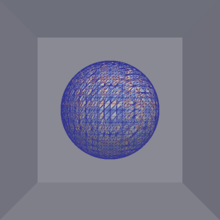
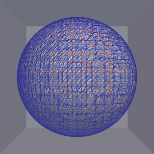
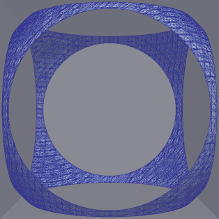
Figure 5. A sequence of reconstructed surface meshes of the immersed growing objects.

To be more precise, the finite element basis functions on the four tetrahedra in each macro-element is constructed as the standard hat function in 3D. On the remaining octahedron, we first add an auxiliary point $6$ near or at the mass center. The octahedron will be sub-divided into $8$ tetrahedra; see Fig. 6 for an illustration. We then construct standard hat functions on each tetrahedron. The extra degree of freedom at the node $6$ will be eliminated by the averaging of the values at nodes $0-5$; see more details in [19, 24]. By this means, we do not introduce new degrees of freedom. The number of total degrees of freedom is the number of nodes plus edges in the original mesh consisting of pure big tetrahedral macro-elements.

Figure 6. Splitting of an octahedron into $8$ tetrahedra $\{0,1,2,6\}$, $\{0,2,3,6\}$, $\{0,3,4,6\}$, $\{0,1,4,6\}$, $\{5,1,4,6\}$, $\{5,1,2,6\}$, $\{5,2,3,6\}$, $\{5,3,4,6\}$: Original edges (thick lines), added edges (thin lines), original nodes $\{0-5\}$, added node $\{6\}$.

4. Solution methods for the linear system of equations

4.1. An all-at-once method

After using finite element discretization, at each time step, we obtain the following linear system of equations:

(5) $$Ku=\left[\begin{array}[]{cc}A_{VV}&A_{VE}\\ A_{EV}&A_{EE}\end{array}\right]\left[\begin{array}[]{c}u_{V}\\ u_{E}\end{array}\right]=\left[\begin{array}[]{c}f_{V}\\ f_{E}\end{array}\right]=f.$$

We solve the linear system of equations by the AMG preconditioned conjugate gradient (PCG) method (see, e.g., [11]) and the AMG preconditioned GMRES method (see [20]). We mention here that, due to the small convection term, we found out that even the PCG method works well for solving such a non-symmetrically perturbed symmetric linear system of equations. For convenience of the solution procedure, the linear system has been ordered with firstly the degrees of freedom on the original tetrahedral nodes $u_{V}$, and then of the edges $u_{E}$, where the subscripts $V$ and $E$ are associated with the nodes and edges. Such reordering has been used in the AMG method for high-order finite element discretized equations [23, 15]. The stiffness matrices $A_{VV}$ and $A_{EE}$ arise from the finite element assembly of the basis functions associated with the original macro-element nodes and edges, respectively, $A_{EV}$ and $A_{VE}$ are coming from the coupling. To solve such a linear system of equations, we use a special AMG method [14], that is based on the matrix graph connectivity. Similar idea was also developed in [3]. In our numerical simulation, such solution methods give us quite satisfactory results. We observe a quite robust behavior of the AMG preconditioner with respect to moving interface in each time step.

4.2. A segregated method

By a close look at the matrix structure in (5), we have observed that $A_{VV}$ is a block-diagonal matrix. This is due to the fact that the degrees of freedom associated with the original macro-element nodes are completely decoupled. In Fig. 7, we demonstrate a sparsity pattern of the system matrix $K$, where it is easy to see the block-diagonal structure of $A_{VV}$.

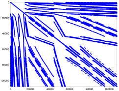
Figure 7. Sparsity pattern of the system matrix $K$.

We now perform a $LU$ factorization of the system matrix $K$ in (5):

(6) $$K=LU=\left[\begin{array}[]{cc}A_{VV}&0\\ A_{EV}&S\end{array}\right]\left[\begin{array}[]{cc}I&A_{VV}^{-1}A_{VE}\\ 0&I\end{array}\right],$$

where $S$ denotes the Schur complement $S=A_{EE}-A_{EV}A_{VV}^{-1}A_{VE}$. Since $A_{VV}^{-1}$ can be constructed very easily, the Schur complement $S$ can also be constructed exactly. A simple blockwise forward and backward substitution gives rise to the solution of the linear system. The main cost is to solve the Schur complement equation

(7) $$Sx_{EE}=b_{E}$$

for $b_{E}:=f_{E}-A_{EV}A_{VV}^{-1}f_{V}$. This is realized by applying the AMG preconditioned CG method [11].

5. Numerical results

5.1. The numerical result for the model problem with an immersed moving sphere

In the first example, we consider a sphere with fixed radius $0.12$ and the initial center at $(0.125,0.125,0.125)$ immersed in a unit cube; see Fig. 8 for an illustration.

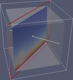
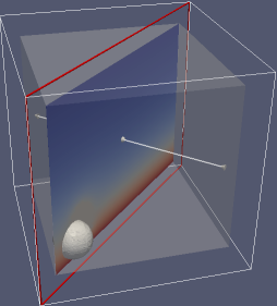
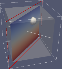
Figure 8. Cutting plane (left), constructed moving sphere surfaces at the time $t=0$ (middle) and $t=0.5625$ (right).

The cube is decomposed into macro-elements with $35937$ nodes and $196608$ tetrahedra. The sub-divided hybrid mesh consists of $274625$ nodes and $786432$ tetrahedra and $196608$ octahedra. The total number of degrees of freedom is $823875$. See Fig. 9 for an illustration.

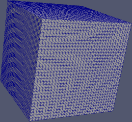
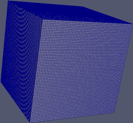
Figure 9. Original pure tetrahedral mesh (left), the sub-divided mesh (right).

The sphere is moving along the line with the starting point $(0,0,0)$ and the ending point $(1,1,1)$, and the moving speed is $v=(1,1,1)^{T}$. The constructed sphere surface is shown in the middle and right plots of Fig. 8. On the bottom of the cube, we set the Dirichlet boundary condition $u=(0,0,0)^{T}$, on the top, $u=(1,0,0)^{T}$. For the rest of the boundaries, we use the homogeneous Neumann boundary condition. The time stepsize is $\Delta t=0.0625$ and the number of time steps is $9$, i.e., the ending time is $T=0.5625$. The material coefficient inside $\Omega_{1}^{t}$ is $a_{1}=1.0e+06$ and inside $\Omega_{2}^{t}$ is $a_{1}=1.0$. The simulation results at different time on the cutting plane (see the left plot in Fig. 8) are shown in Fig. 10. The relative residual error is set to $10e-09$ as stopping criteria. The iteration numbers and the computational CPU time (in second) of the AMG preconditioned CG and GMRES methods in the all-at-once method, and the iteration numbers of the AMG preconditioned CG for the Schur complement equation and the computational CPU time in the segregated method, are shown in Fig. 11. We observe that, in terms of iteration numbers, the GMRES method shows the best performance, then the CG method, and last the segregated method. However, regarding CPU time, we see that, the CG method shows its best performance, then the segregated method, and last the GMRES.

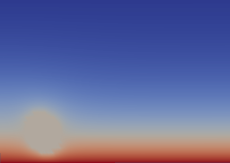
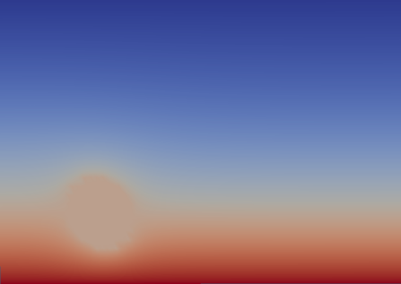
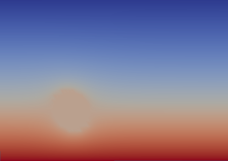
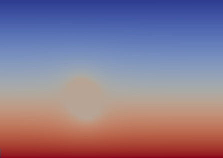
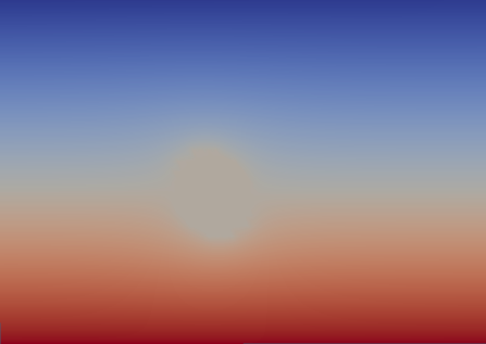
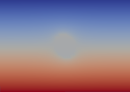
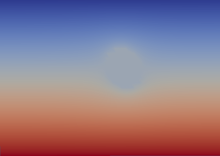
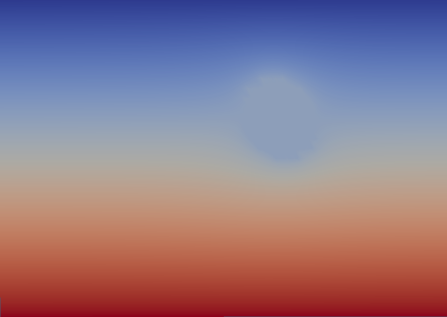
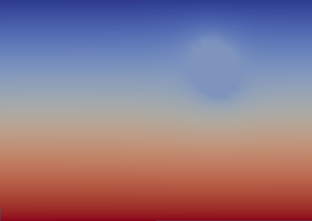
Figure 10. Simulation results with the moving object in the domain at different time levels $t=0.0625k$, $k=1,...,9$, on the cutting face.

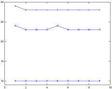
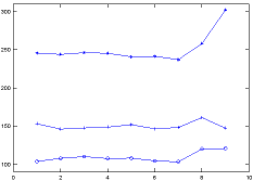
Figure 11. Iteration numbers (left) and CPU time measured in second $s$ (right) for solving the time dependent heat equation with the immersed moving object in each time step: AMG preconditioned CG (solid lines with circle markers), AMG preconditioned GMRES (solid lines with star markers) in the monolithic method, AMG preconditioned CG (solid lines with plus markers) for the Schur complement equation in the segregated method.

5.2. The numerical result for the model problem with an immersed growing sphere

In the second example, we consider a sphere with an initial radius $0.08$ and the initial center at $(0.5,0.5,0.5)$ immersed in a unit cube; see Fig. 12 for an illustration. We use the same finite element mesh as in the first example. The sphere is growing along the radius direction and the growing speed is $v=n$, where $n$ denotes the outward unit normal vector in the radius direction. The surfaces of the growing sphere at time $t=0$ and $t=0.45$ are constructed as shown in the middle and right plots of Fig. 12, respectively. On the bottom of the cube, we set the Dirichlet boundary conditions $u=(0,0,0)^{T}$, on the top, $u=(1,0,0)^{T}$. For the rest of the boundaries, we use the homogeneous Neumann boundary condition. The time stepsize is $\Delta t=0.05$ and the number of time steps is $9$, i.e., the ending time is $T=0.45$. The material coefficient inside $\Omega_{1}^{t}$ is $a_{1}=1.0e+06$ and inside $\Omega_{2}^{t}$ is $a_{1}=1.0$. The simulation results on the cutting plane (see the left plot in Fig. 12) is shown in Fig. 13. The relative residual error is set to $10e-09$ as stopping criteria of the linear solvers. The iteration numbers and the computational CPU time (in second) of the AMG preconditioned CG and GMRES methods in the all-at-once method, and the iteration numbers of the AMG preconditioned CG for the Schur complement equation and the computational CPU time in the segregated method, are shown in Fig. 14. We observe that, in terms of iteration numbers, the GMRES method shows the best performance, then the CG method, and last the segregated method. However, regarding CPU time, we see that again, the CG method shows the best performance, then the segregated method, and last the GMRES method.

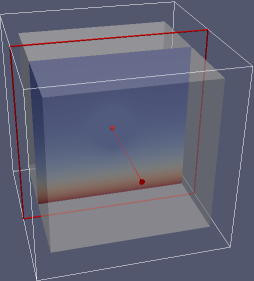
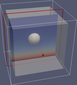
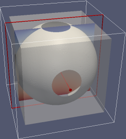
Figure 12. Cutting plane (left), constructed growing sphere surfaces at time $t=0$ (middle) and $t=0.45$ (right).

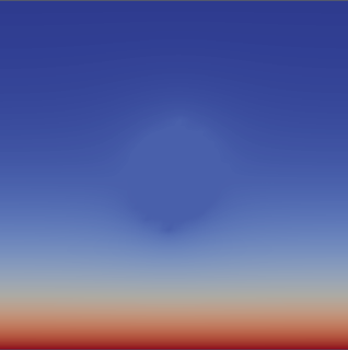
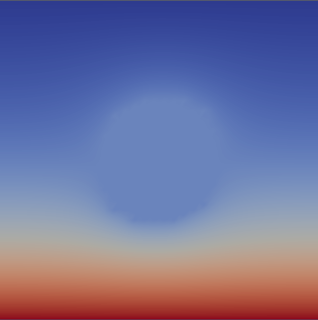
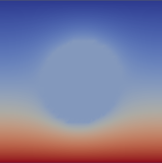
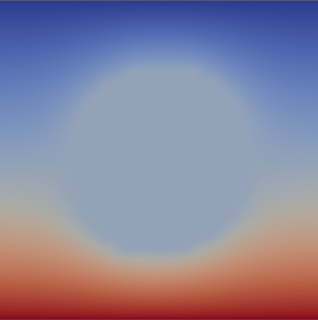
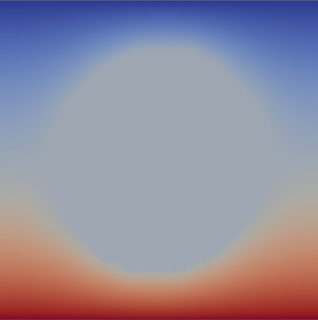
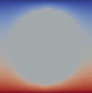
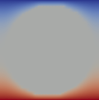
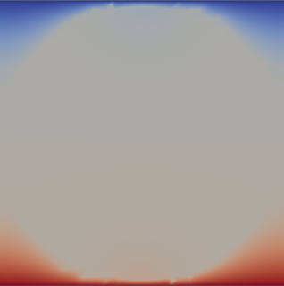
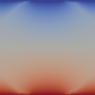
Figure 13. Simulation results with the growing object in the domain at different time levels $t=0.05k$, $k=1,...,9$, on the cutting face.

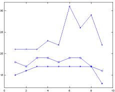
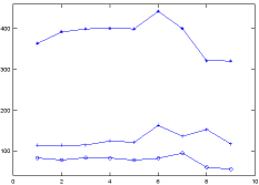
Figure 14. Iteration numbers (left) and CPU time measured in second $s$ (right) for solving the time dependent heat equation with the immersed growing object in each time step: AMG preconditioned CG (solid lines with circle markers), AMG preconditioned GMRES (solid lines with star markers) in the monolithic method, AMG preconditioned CG (solid lines with plus markers) for the Schur complement equation in the segregated method.

6. Conclusion

In this work, we develop an ALE method on the underlying reference domain decomposed macro-elements consisting of tetrahedral and octahedral elements. That is combined with the interface capturing method. The numerical results demonstrate the robustness of this method with respect to large displacement or deformation of the moving interface in the model parabolic problem. We have compared the algebraic multigrid based all-at-once and the segregated methods for solving the linear system of algebraic equations arising from the finite element discretization. We observed that the all-at-once AMG preconditioned CG method shows the best performance in terms of CPU time. The segregated method shows comparable performance. Regarding the iteration numbers, the AMG preconditioned GMRES method shows the best performance.

References

- [1] J. Baiges and R. Codina, The fixed-mesh ALE approach applied to solid mechanics and fluid-structure interaction problems, Int. J. Numer. Meth. Engng., 81 (2010), pp. 1529–1557.
- [2] D. Boffi, N. Cavallini, and L. Gastaldi, Finite element approach to immersed boundary method with different fluid and solid densities, M3AS, 21 (2011), pp. 2523–2550.
- [3] D. Braess, Towards algebraic multigrid for elliptic problems of second order, Computing, 55 (1995), pp. 379–393.
- [4] J. H. Bramble and J. King, A finite element method for interface problems in domains with smooth boundaries and interfaces, Advances Comput. Math., 6 (1996), pp. 109–138.
- [5] Z. Chen and J. Zou, Finite element methods and their convergence for elliptic and parabolic interface problems, Numer. Math., 79 (1998), pp. 175–202.
- [6] R. Codina, G. Houzeaux, H. Coppola-Owen, and J. Baiges, The fixed-mesh ALE approach for the numerical approximation of flows in moving domains, J. Comput. Physics, 228 (2009), pp. 1591–1611.
- [7] J. Donea, A. Huerta, J. Ponthot, and A. Ferran, Arbitrary Lagrangian-Eulerian methods, in The Encyclopedia of Computational Mechanics, E. Stein, R. Borst, and T. Hughes, eds., vol. 1, Wiley& Sons, Ltd, 2004, pp. 413–437.
- [8] S. Frei and T. Richter, A locally modified parametric finite element method for interface problems, SIAM J. Numer. Anal., 52 (2014), pp. 2315–2334.
- [9] A. Gerstenberger and W. A. Wall, Enhancement of fixed-grid methods towards complex fluid-structure interaction applications, Int. J. Numer. Meth. Fluids, 57 (2008), pp. 1227–1248.
- [10] Y. Gong, B. Li, and Z. Li, Immersed-interface finite-element methods for elliptic interface problems with nonhomogeneous jump conditions, SIAM J. Numer. Anal., 46 (2008), pp. 472–495.
- [11] G. Haase and U. Langer, Modern Methods in Scientific Computing and Applications, vol. 75 of NATO Science Series II. Mathematics, Physics and Chemistry, Kluwer Academic Press, Dordrecht, 2002, ch. Multigrid Methods: From Geometrical to Algebraic Versions, pp. 103–154.
- [12] T. Hughes, W. Liu, and T. Zimmermann, Lagrangian-Eulerian finite element formulation for incompressible viscous flows, Comput. Methods Appl. Mech. Engrg., 29 (1981), pp. 329–349.
- [13] E. Karabelas and M. Neumüller, Generating admissible space-time meshes for moving domains in d+1-dimensions, Tech. Rep. 2015-07, Institute for Computational Mathematics, Johannes Kepler University Linz, 2015. http://www.numa.uni-linz.ac.at/publications/List/2015/2015-07.pdf.
- [14] F. Kickinger, Algebraic multigrid for discrete elliptic second-order problems, in Multigrid Methods V. Proceedings of the 5th European Multigrid conference (ed. by W. Hackbush), Lecture Notes in Computational Sciences and Engineering, vol. 3, Springer, 1998, pp. 157–172.
- [15] U. Langer and H. Yang, Algebraic multigrid based preconditioners for fluid-structure interaction and its related sub-problems, in The 10th International Conference on Large-Scale Scientific Computations, Springer, 2015. accepted.
- [16] Z. Li, T. Lin, and X. Wu, New Cartesian grid methods for interface problems using the finite element formulation, Numer. Math., 96 (2003), pp. 61–98.
- [17] M. Neumüller and O. Steinbach, Refinement of flexible space-time finite element meshes and discontinuous Galerkin methods, Comput. Visual. Sci., 14 (2011), pp. 189–205.
- [18] M. Razzaq, H. Damanik, J. Hron, A. Ouazzi, and S. Turek, FEM multigrid techniques for fluid-structure interaction with application to hemodynamics, Appl. Numer. Math., 62 (2012), pp. 1156–1170.
- [19] B. Rocha, F. Kickinger, A. Prassl, G. Haase, E. J. Vigmond, R. Weber dos Santos, S. Zaglmayr, and G. Plank, A macro finite-element formulation for cardiac electrophysiology simulations using hybrid unstructured grids, IEEE Trans. Biomed. Eng., 58 (2011), pp. 1055–1065.
- [20] Y. Saad and M. H. Schultz, GMRES: A generalized minimal residual algorithm for solving nonsymmetric linear systems, SIAM J. Sci. Stat. Comput., 7 (1986), pp. 856–869.
- [21] T. Wick, Fluid-structure interactions using different mesh motion techniques, Comput. Structures, 89 (2011), pp. 1456–1467.
- [22] H. Yang, Partitioned solvers for the fluid-structure interaction problems with a nearly incompressible elasticity model, Comput. Visual. Sci., 14 (2011), pp. 227–247.
- [23] , An algebraic multigrid method for quadratic finite element equations of elliptic and saddle point systems in 3d, arxiv.org/abs/1503.01287, (2015).
- [24] H. Yang and W. Zulehner, Numerical simulation of fluid-structure interaction problems on hybrid meshes with algebraic multigrid methods, J. Comput. Appl. Math., 235 (2011), pp. 5367–5379.