Topological vortices in generalized Born-Infeld-Higgs electrodynamics

Abstract

A consistent BPS formalism to study the existence of topological axially symmetric vortices in generalized versions of the Born-Infeld-Higgs electrodynamics is implemented. Such a generalization modifies the field dynamics via introduction of three non-negative functions depending only in the Higgs field, namely, $G(|\phi|)$, $w(|\phi|)$ and $V(|\phi|)$. A set of first-order differential equations is attained when these functions satisfy a constraint related to the Ampere law. Such a constraint allows to minimize the system energy in such way that it becomes proportional to the magnetic flux. Our results provides an enhancement of topological vortex solutions in Born-Infeld-Higgs electrodynamics. Finally, we analyze a set of models such that a generalized version of Maxwell-Higgs electrodynamics is recovered in a certain limit of the theory.

I Introduction

The well-known Born-Infeld electrodynamics was originally introduced to remove the divergence of electron’s self-energy in classical electrodynamics by introducing a square-root form of the Lagrangian density replacing the standard Maxwell Lagrangian BI . In this way the field strength tensor remains bounded everywhere and the energy associated to a point-like charge becomes finite. This theory is a distinguished member of the family of nonlinear electrodynamics since it enjoys three properties: i) Maxwell weak-field limit, ii) electric-magnetic duality em-duality , and iii) absence of shock waves and birefringence phenomena concerning propagation of waves, belonging to the class of theories called “completely exceptional” wave . Applications of Born-Infeld electrodynamics within gravitation and cosmology have been considered for many years BI-applications . This model is moreover deemed of a special attention since it appears in the low-energy limit of string/D-Branes physics D-branes1 ; D-branes2 ; D-branes3 .

On the other hand, the study of magnetic vortices gained great interest since Abrikosov’s description for Type-II superconductors Abrikosov , which arise naturally from the non-relativistic limit of Ginzburg-Landau (GL) theory GL . In field theory, stable vortex configurations came up with the seminal work by Nielsen and Olesen NO whose study of the Maxwell-Higgs (MH) model shows that electrically neutral vortex solutions correspond to the ones obtained by Abrikosov. Lately it was verified the existence of electrically charged vortex solutions in Chern-Simons-Higgs (CSH) CS ; CSV and Maxwell-Chern-Simons-Higgs (MCSH) MCS ; Bolog models. In all these cases, the presence of the Higgs fields is essential for the existence of vortex-type solutions.

Recently, it has been intensively studied the existence of topological defects in generalized or new effective field theories. For example one can introduce noncanonical kinetic terms o1 ; Hora_Rubiera , in order to circumvent the constraints of Derrick’s theorem Derrick and obtain topological defect solutions (see e.g. Books for a more detailed account on soliton-like solutions in field theory). Other models are defined by introducing generalizing functions on standard field models o2 . In some cases these generalized models provide self-dual analytical solutions which certainly enriches our understanding of the field PLB ; AHEP . Moreover, this procedure allows to control properties of the topological defect, such as its width or energy density, providing valuable models for the analysis of several physical problems. In the literature there are many interesting applications of these new solutions within several different scenarios, specially involving the accelerated inflationary phase of the universe n8 via the so-called k-essence models shutt , strong gravitational waves sgw , tachyon matter tm , dark matter dm , and other topics o .

Among generalized models the simplest ones are those generalizing the Maxwell-Higgs model gmh , Chern-Simons-Higgs model gcsh and Maxwell-Chern-Simons-Higgs model gmcsh . Based on earlier work on vortices in Born-Infeld-Higgs models Shiraishi , in Ref. Hora_Rubiera a generalization of Born-Infeld-Maxwell-Higgs (BIMH) model was constructed within the context of generalized dynamics, but self-dual or BPS vortices were not found. The main aim of the present manuscript is to show the existence of self-dual topological BPS vortices in a generalized BIMH electrodynamics, and study their properties.

II Generalized Born-Infeld vortices

The Lagrangian density of our ($2+1$)-dimensional theory is written as

$$\mathcal{L}=\beta^{2}\left(1-\mathcal{R}\right)+w\left(\left|\phi\right|\right)\left|D_{\mu}\phi\right|^{2}-W\left(\left|\phi\right|\right)\text{,}$$ (1)

with the definitions

$$\mathcal{R} = \sqrt{1+\frac{G\left(\left|\phi\right|\right)}{2\beta^{2}}F_{\mu\nu}F^{\mu\nu}},$$ (2)

$$W\left(\left|\phi\right|\right) = \beta^{2}\left[1-V\left(\left|\phi\right|\right)\right],$$ (3)

where $F_{\mu\nu}=\partial_{\mu}A_{\nu}-\partial_{\nu}A_{\mu}$ is the field strength tensor of the vector potential $A_{\mu}$, while the covariant derivative realizing the coupling between the gauge and Higgs fields is given by $D_{\mu}\phi=\partial_{\mu}\phi-ieA_{\mu}\phi$. The positive functions $G\left(\left|\phi\right|\right)$ and $w\left(\left|\phi\right|\right)$ are the generalizing functions in the kinetic sector. The generalized potential $W\left(\left|\phi\right|\right)$, a nonnegative function, inherits its structure from the function $V(|\phi|)$, which is restricted by the condition $0<V(|\phi|)\leq 1$, so $W(\phi)>0$. The Born-Infeld parameter, $\beta$, provides modified dynamics for both scalar and gauge fields further enriching the family of possible models.

From the action (1) the gauge field equations of motion read

$$\partial_{\nu}\left(\frac{G}{\mathcal{R}}F^{\nu\mu}\right)=ewJ^{\mu},$$ (4)

where $J^{\mu}=i(\phi\partial^{\mu}\phi^{\ast}-\phi^{\ast}\partial^{\mu}\phi)-2eA^{\mu}\left|\phi\right|^{2}$ plays the role of a current.

At static regime, Eq. (4) provides the Gauss law,

$$\partial_{j}\left(\frac{G}{\mathcal{R}}\partial_{j}A_{0}\right)=2we^{2}A_{0}\left|\phi\right|^{2},$$ (5)

which is saturated by temporal gauge: $A_{0}=0$. In this way we see that the model, at static regime and in temporal gauge, describes electrically neutral magnetic configurations. Under these conditions, from Eq. (4) the Ampere law reads

$$\epsilon_{kj}\partial_{j}\left(\frac{G}{\mathcal{R}}B\right)-ewJ_{k}=0,$$ (6)

and Higgs’s field equation becomes

$$0 = w\left(D_{j}D_{j}\phi\right)+\left(\partial_{j}w\right)D_{j}\phi$$

$$-\frac{\partial w}{\partial\phi^{\ast}}\left|D_{j}\phi\right|^{2}-\frac{B^{2}}{\ 2\mathcal{R}}\frac{\partial G}{\partial\phi^{\ast}}-\frac{\partial W}{\partial\phi^{\ast}},$$

where in the last two equations $\mathcal{R}$ reads

$$\mathcal{R}=\left(1+\frac{G}{\beta^{2}}B^{2}\right)^{1/2}.$$ (8)

The energy-momentum tensor of the model is given by

$$T_{\mu\nu} = -\frac{1}{\mathcal{R}}G\left(\left|\phi\right|\right)F^{\beta}{}_{\mu}F_{\beta\nu}+w\left(\left|\phi\right|\right)\left(D_{\mu}\phi\right)^{\ast}D_{\nu}\phi$$ (9)

$$+w\left(\left|\phi\right|\right)\left(D_{\nu}\phi\right)^{\ast}D_{\mu}\phi-g_{\mu\nu}\mathcal{L}.$$

In this work we are interested in searching for electrically neutral magnetic vortices and, more specifically, we will study such solutions at static regime and in temporal gauge. As it is largely known in literature, the axially symmetric vortex ansatz works fine to find such solutions, namely,

$$\phi=vg\left(r\right)e^{in\theta},\leavevmode\nobreak\ A_{\theta}=-\frac{a\left(r\right)-n}{er},$$ (10)

where $n$ is an integer number and $a(r)$ and $g(r)$ are regular functions that satisfy the following boundary conditions

$$g\left(0\right) = 0\leavevmode\nobreak\ ,\leavevmode\nobreak\ \ \ g\left(\infty\right)=1$$ (11)

$$a\left(0\right) = n\leavevmode\nobreak\ ,\leavevmode\nobreak\ \ \ a\left(\infty\right)=0$$ (12)

Using this ansatz the magnetic field is written as

$$B=-\frac{a^{\prime}}{er}.$$ (13)

with the short-hand notation $a^{\prime}\equiv da/dr$.

For the ansatz (10) the Ampere law (6) is expressed as

$$\left(\frac{G}{\mathcal{R}}B\right)^{\prime}=-2ev^{2}w\frac{ag^{2}}{r},$$ (14)

while Higgs’ field equation (LABEL:eq:Higgs) reads

$$0 = g^{\prime\prime}+\frac{g^{\prime}}{r}-\frac{a^{2}}{r^{2}}g+\frac{1}{2w}\frac{dw}{dg}\left[\left(g^{\prime}\right)^{2}-\left(\frac{ag}{r}\right)^{2}\right]$$

$$-\frac{1}{4wv^{2}}\frac{B^{2}}{\mathcal{R}}\frac{dG}{dg}-\frac{1}{2wv^{2}}\frac{dW}{dg},$$

where $\mathcal{R}$ is given by Eq.(8).

II.1 The BPS formalism

The energy of the vortex is given by the integration of the $T_{00}$ component of (9) which, in static regime and in the gauge $A_{0}=0$, is given by

$$T_{00}=\beta^{2}\left(\mathcal{R}-V\right)+wv^{2}\left(g^{\prime}\right)^{2}+wv^{2}\left(\frac{ag}{r}\right)^{2},$$ (16)

and will be nonnegative whenever the condition $\mathcal{R}\geq V$ is satisfied. The total energy reads

$$E=2\pi\!\int\!\!drr\!\left[\beta^{2}\left(\mathcal{R}-V\right)+wv^{2}\left(g^{\prime}\right)^{2}+wv^{2}\left(\frac{ag}{r}\right)^{2}\right],$$ (17)

where the fields were expressed in terms of the ansatz (10). We now use the Bogomol’nyi trick Bogol to rewrite it as

$$E = 2\pi\!\int\!\!drr\left[\frac{1}{2}\frac{G}{\mathcal{R}}\left(B\mp\beta\sqrt{\frac{2F}{G}}\right)^{2}+wv^{2}\left(g^{\prime}\mp\frac{ag}{r}\right)^{2}\right.$$

$$\hskip 56.9055pt\pm B\frac{\beta}{\mathcal{R}}\sqrt{2FG}\pm 2wv^{2}\frac{ag}{r}g^{\prime}$$

$$\hskip 56.9055pt\left.+\beta^{2}\mathcal{R}-\frac{1}{2}\frac{GB^{2}}{\mathcal{R}}-\frac{\beta^{2}F}{\mathcal{R}}-\beta^{2}V\right],$$

where we have introduced the function $F$, which is, in principle, arbitrary but nonnegative, to be determined later in order to obtain solutions with well defined energy. Using the definition (8) in the third row, we can rewrite (II.1) as

$$E = 2\pi\!\int\!\!drr\left\{\pm B\frac{\beta}{\mathcal{R}}\sqrt{2FG}\pm 2wv^{2}\frac{ag}{r}g^{\prime}\right.$$

$$+\frac{1}{2}\frac{G}{\mathcal{R}}\left(B\mp\beta\sqrt{\frac{2F}{G}}\right)^{2}+wv^{2}\left(g^{\prime}\mp\frac{ag}{r}\right)^{2}$$

$$\left.+\frac{\beta^{2}}{\mathcal{R}}\left[\frac{1}{2}\left(\mathcal{R}-V\right)^{2}+\frac{1}{2}\left(1-V^{2}\right)-F\right]\right\}.$$

We observe that, by imposing the expression in the third row to be null, this allows to determine the function $F$ in terms of $V$ and $R$, namely

$$F=\frac{1}{2}\left(\mathcal{R}-V\right)^{2}+\frac{1}{2}\left(1-V^{2}\right),$$ (20)

which shows that $F$ is a nonnegative function because $0<V\leq 1$. Let us point out that the function $F$ is defined without considering the self-dual equations or the BPS limit.

Now by considering condition (20) and the expression (13) for the magnetic field, the energy (II.1) reads

$$E = 2\pi\!v^{2}\int\!\!drr\left\{\mp\frac{a^{\prime}}{r}\left(\frac{\beta\sqrt{2FG}}{ev^{2}\mathcal{R}}\right)\mp\frac{a}{r}\left(-2wgg^{\prime}\right)\right.$$

$$\hskip 14.22636pt\left.+\frac{1}{2}\frac{G}{\mathcal{R}}\left(B\mp\beta\sqrt{\frac{2F}{G}}\right)^{2}+wv^{2}\left(g^{\prime}\mp\frac{ag}{r}\right)^{2}\right\}.$$

We can now transform the first term in a total derivative by setting

$$\left(\frac{\beta}{ev^{2}\mathcal{R}}\sqrt{2FG}\right)^{\prime}=-2wgg^{\prime},$$ (22)

This way, the energy (II.1) is written as

$$E = 2\pi\!v^{2}\!\int\!\!drr\left[\mp\frac{1}{r}\left(a\Omega\right)^{\prime}\right.$$

$$\leavevmode\nobreak\ \ \ \ \ \ \leavevmode\nobreak\ \ \ \ \left.wv^{2}\left(g^{\prime}\mp\frac{ag}{r}\right)^{2}+\frac{1}{2}\frac{G}{\mathcal{R}}\left(B\mp\beta\sqrt{\frac{2F}{G}}\right)^{2}\right],$$

where

$$\Omega=\frac{\beta}{ev^{2}\mathcal{R}}\sqrt{2FG},$$ (24)

with the function $F$ given by Eq. (20). We can now further constrain the set of functions $G$, $w$ and $V$ in order to attain a true lower bound for the energy by selecting functions satisfying

$$\Omega\left(0\right)=1,\leavevmode\nobreak\ \Omega\left(\infty\right)=\text{finite}$$ (25)

Then, by considering the boundary conditions given by Eqs. (25) and (11), the energy reads

$$E = 2\pi v^{2}\left|n\right|$$

$$+2\pi\!\int\!\!drr\left[wv^{2}\left(g^{\prime}\mp\frac{ag}{r}\right)^{2}+\frac{1}{2}\frac{G}{\mathcal{R}}\left(B\mp\beta\sqrt{\frac{2F}{G}}\right)^{2}\right].$$

This clearly shows that the energy possess a lower bound

$$E\geq 2\pi v^{2}\left|n\right|,$$ (27)

whenever the functions $G$, $w$ and $V$ chosen provide a function $\Omega$ satisfying Eq. (25). Such a lower bound is saturated when the fields satisfy the BPS or self-dual equations

$$g^{\prime}=\pm\frac{ag}{r},$$ (28)

$$B=\pm\frac{\beta}{V}\sqrt{\frac{1-V^{2}}{G}}.$$ (29)

This is a set of first-order equations that satisfy automatically the second-order equations (14) and (II), as can be immediately seen by derivation of the former. This is so because the Euler-Lagrangian equations only imply that a static BPS solution will be a stationary point of the energy. In Eq.(29) we have used (20) to compute $F$ in the BPS limit, which provides

$$F=\frac{1-V^{2}}{2V^{2}},$$ (30)

a nonnegative function due to $0<V\leq 1$. Similarly, the nonnegative function $\Omega\left(r\right)$ is given by

$$\Omega_{bps}=\beta\sqrt{G\left(1-V^{2}\right)}.$$ (31)

By using the BPS equations (28) and (29), Ampere’s law (14) can be written as

$$\frac{d}{dg}\sqrt{\beta^{2}G\left(1-V^{2}\right)}=-2ev^{2}wg.$$ (32)

This relation allows to determine one of the generalizing functions when the other two are given, for example, we can compute $w$ if we provide the functions $G$ and $V$. Here it is worthwhile to notice that Eq.(32) is exactly the condition (22) in the BPS limit.

To conclude this section, the BPS energy density of the model, which appears in

$$E_{bps}=\displaystyle{2\pi\!\int\!\!drr\leavevmode\nobreak\ \varepsilon_{bps},}$$ (33)

is given by

$$\varepsilon_{bps}=\frac{\beta^{2}}{V}\left(1-V^{2}\right)+2wv^{2}\left(\frac{ag}{r}\right)^{2}.$$ (34)

and will be positive definite whenever the functions $0<V\left(g\right)\leq 1$ and $w\left(g\right)\geq 0$.

III A family of models

In this section we shall focus on the special case

$$V\left(\left|\phi\right|\right)=\sqrt{1-\frac{2U\left(\left|\phi\right|\right)}{\beta^{2}}},$$ (35)

since this choice, in the limit $\beta\rightarrow\infty$, allows to obtain the generalized Maxwell-Higgs model from the Lagrangian density (1):

$$\mathcal{L}=-\frac{G\left(\left|\phi\right|\right)}{4}F_{\mu\nu}F^{\mu\nu}+w\left(\left|\phi\right|\right)\left|D_{\mu}\phi\right|^{2}-U\left(\left|\phi\right|\right).$$ (36)

With this choice the BPS equations read

$$g^{\prime} = \pm\frac{ag}{r},\leavevmode\nobreak\$$ (37)

$$B = \pm\sqrt{\frac{2U}{G}}\left(1-\frac{2U}{\beta^{2}}\right)^{-1}.$$ (38)

The condition (32) reads

$$\frac{d}{dg}\sqrt{2UG}=-2ev^{2}wg,$$ (39)

and the BPS energy density is

$$\varepsilon_{bps}=2U\left(1-\frac{2U}{\beta^{2}}\right)^{-1/2}+2v^{2}w\left(\frac{ag}{r}\right)^{2}.$$ (40)

Therefore, the generalized models can be defined by choosing $G\left(g\right)$ and $U\left(g\right)$ functions which, via the constraint (39), allow to find the remaining function $w\left(g\right)$. These three functions must be nonnegative for positive definiteness of the energy density. In the next sections we shall choose some models satisfying the constraint (25) and, therefore, their BPS solutions will saturate the bound (27).

III.1 Some choices for the potential

Next we shall consider two classes of models characterized by the form of the “potential” $\leavevmode\nobreak\ U(g)$. First we will consider, in each case, the asymptotic behavior of the functions $g(r)$ and $a(r)$ compatible with the boundary conditions that make the energy finite and positive, and next solve the BPS equations. On the other hand we note that $\beta$ is not a constant characterizing the solutions but rather a parameter determining a particular model within the family defined by the corresponding term in the action (1). In some of the following numerical cases we shall treat nevertheless $\beta$ as a free parameter for the computations, which means that in those cases we will be comparing the behavior of the solutions corresponding to different models of the family of generalized Born-Infeld Lagrangians. In order to perform the numerical analysis, without loss of generality, we set $e=1=v$.

III.2 Asymptotic behavior for $\left|\phi\right|^{4}$ models

The $\left|\phi\right|^{4}$-models are described by the function $U\left(g\right)$ given by

$$U\left(g\right)=\frac{1}{2}\left(1-g^{2}\right)^{2},$$ (41)

and the function $G\left(g\right)$ whose behavior when $r\rightarrow 0$ is

$$G\left(g\right)=\alpha_{0}+\alpha_{2}g^{2}+...,$$ (42)

and when $r\rightarrow\infty$ reads

$$G\left(g\right)=\alpha_{0}^{\left(\infty\right)}+\alpha_{1}^{\left(\infty\right)}\left(1-g\right)+\alpha_{2}^{\left(\infty\right)}\left(1-g\right)^{2}+....$$ (43)

where $\alpha_{0},\alpha_{2},\ldots$, and $\alpha_{0}^{\left(\infty\right)},\alpha_{1}^{\left(\infty\right)},\ldots$ are some constants.

By introducing the above information into the BPS equations (37) and (38), we can compute the behavior of field profiles when $r\rightarrow 0$:

$$g\left(r\right) = C_{n}r^{n}-\left(\frac{{\beta}^{2}}{{\beta}^{2}-1}\right)^{1/2}\frac{C_{n}r^{n+2}}{4\left(\alpha_{0}\right)^{1/2}}+...$$ (44)

$$a\left(r\right) = n-\left(\frac{{\beta}^{2}}{{\beta}^{2}-1}\right)^{1/2}\frac{r^{2}}{2\left(\alpha_{0}\right)^{1/2}}$$

$$+\left(\frac{{\beta}^{2}}{{\beta}^{2}-1}\right)^{3/2}\frac{\left(2\alpha_{0}+\alpha_{2}\right){\beta}^{2}-\alpha_{2}}{\left(\alpha_{0}\right)^{3/2}{\beta}^{2}}\frac{{C}_{n}^{2}{r}^{2n+2}}{4\left(n+1\right)}+...$$

where $C_{n}$ is a set of constants.

Similarly, we calculate the behavior of the profiles at infinity:

$$1-g\left(r\right) \sim r^{-1/2}\exp\left[-r\sqrt{2}\left(\alpha_{0}^{\left(\infty\right)}\right)^{-1/4}\right]$$ (46)

$$a\left(r\right) \sim r^{1/2}\exp\left[-r\sqrt{2}\left(\alpha_{0}^{\left(\infty\right)}\right)^{-1/4}\right].$$ (47)

These expansions are fully consistent with the assumed boundary conditions (11) and (12) for the BPS solutions.

III.3 Asymptotic behavior for $\left|\phi\right|^{6}$ models

In this case, the function $U\left(g\right)$ is given by

$$U\left(g\right)=\frac{1}{2}g^{2}\left(1-g^{2}\right)^{2}.$$ (48)

We consider the behavior of function $G$, which at origin takes the form

$$G\left(g\right)=\frac{\gamma_{-2}}{g^{2}}+\gamma_{0}+\gamma_{2}g^{2}+...,$$ (49)

and at infinity is

$$G\left(g\right)=\gamma_{0}^{\left(\infty\right)}+\gamma_{1}^{\left(\infty\right)}\left(1-g\right)+\gamma_{2}^{\left(\infty\right)}\left(1-g\right)^{2}+...$$ (50)

The behavior of the profiles at $r\rightarrow 0$ is

$$g\left(r\right) \sim C_{n}r^{n}-\frac{C_{n}^{3}r^{3n+2}}{4\left(\gamma_{-2}\right)^{1/2}\left(n+1\right)^{2}}+...$$ (51)

$$a\left(r\right) \sim n-\frac{{C}_{n}^{2}r^{2n+2}}{2\left(\gamma_{-2}\right)^{1/2}\left(n+1\right)}$$

$$+\frac{\left(2\gamma_{-2}+\gamma_{0}\right)\beta^{2}-\gamma_{-2}}{4\beta^{2}\left(\gamma_{-2}\right)^{3/2}\left(2n+1\right)}{C}_{n}^{4}{r}^{4\,n+2}+...$$

while the asymptotic behavior for $r\rightarrow\infty$ is

$$1-g\left(r\right) \sim r^{-1/2}\exp\left[-r\sqrt{2}\left(\gamma_{0}^{\left(\infty\right)}\right)^{-1/4}\right]$$ (53)

$$a\left(r\right) \sim r^{1/2}\exp\left[-r\sqrt{2}\left(\gamma_{0}^{\left(\infty\right)}\right)^{-1/4}\right]$$ (54)

and, again, these expansions are consistent with the problem under consideration.

III.4 Discussion of results

Once the boundary conditions are fixed, we have performed numerical solutions of the BPS equations (37) and (38) by using routines of Maple 16.2. The first numerical results are obtained by considering fixed values of $\beta(=1.05)$, and comparing the standard MH, CSH and BIMH models with our $\left|\phi\right|^{4}$-BIMH and $\left|\phi\right|^{6}$-BIMH models. These results are shown in Figs. 1, 2, 3 and 4. The second numerical analysis was performed by fixing $n=1$ and varying the values of $\beta(=1.05,1.25,2.00,\infty$), with the resulting profiles depicted in Figs. 5, 6, 7 and 8 for the $\left|\phi\right|^{4}$-BIMH and $\left|\phi\right|^{6}$-BIMH models studied in this work. In both scenarios, we have depicted the field profiles $g(r)$, $a(r)$, the magnetic field $B(r)$ and the BPS energy density $\varepsilon_{bps}(r)$ corresponding to the different models under comparison.

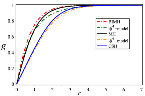
Figure 1: Higgs field ${g}(r)$, for $n=1$ and dashed-dotted lines for $\beta=1.5$.

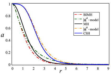
Figure 2: Gauge field profile ${a}(r)$, for $n=1$ and dashed-dotted lines for $\beta=1.5$.

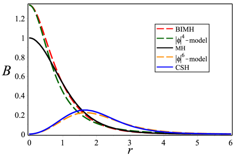
Figure 3: Magnetic field profiles ${B}(r)$, for $n=1$ and dashed lines for $\beta=1.5$.

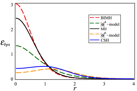
Figure 4: BPS energy density ${\varepsilon}_{{}_{bps}}(r)$, for $n=1$ and dashed lines for $\beta=1.5$.

To further clarify the plots, we note that the first $\phi^{4}$-model is defined by

$$G=1,\leavevmode\nobreak\ w=1,$$ (55)

and represents the standard Born-Infeld-Maxwell-Higgs model (dashed-dotted red lines in Figs. 1–4).

The second one (dashed-dotted green lines in Figs. 1–4) is given by the following functions

$$G\left(g\right)=\exp\left(2g^{2}\right),\ w\left(g\right)=g^{2}\exp\left(2g^{2}\right)$$ (56)

The $\phi^{6}$-model (dashed-dotted orange lines in Figs. 1–4) is defined by the functions

$$G\left(g\right)=\frac{\left(3+g^{2}\right)^{2}}{9g^{2}},\leavevmode\nobreak\ w\left(g\right)=\frac{2}{3}\left(1+g^{2}\right).$$ (57)

For completeness, we also depict the profiles of the standard MH (solid black line) and CSH models (solid blue line).

In general we see that the introduction of a finite value for $\beta$ has a non-trivial impact on the profiles of $a(r)$ and $g(r)$. This follows from the comparison between the standard $\phi^{4}$ BIMH model in Eq. (55) (red dashed curve, corresponding to $\beta=1.5$) and the standard MH system (solid black curve), with the former vortex being ticker than the latter. We also see that the impact of changing the $G$ and $\omega$ functions through the new $\left|\phi\right|^{4}$ and $\left|\phi\right|^{6}$-BIHM models introduced in this work is to made the vortex even more thicker (green and orange curves, corresponding to models (56) and (57), respectively). This is also reflected in the physical magnitudes characterizing the vortex, as both the magnetic field and the energy density profiles (see Figs. 3 and 4, respectively) undergo large modifications as compared to their standard counterparts. In general this means that, at fixed $\beta$, one can control thickness and physical magnitudes of the vortex by introduction of suitable $G$ and $\omega$ functions.

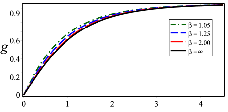
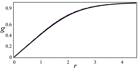
Figure 5: Higgs field profile $g(r)$, for $n=1$. Upper figure represents the $|\phi|^{4}$-model defined by Eq. (56) and the bottom figure represents the $|\phi|^{6}$-model defined in Eq. (57).

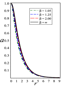
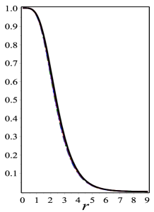
Figure 6: Gauge field profile $a(r)$, for $n=1$. Left figure represents the $|\phi|^{4}$-model defined by Eq. (56) and right-figure represents the $|\phi|^{6}$-model defined in Eq. (57).

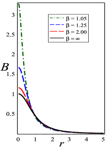
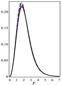
Figure 7: Magnetic field $B(r)$, for $n=1$. Left figure represents the $|\phi|^{4}$-model defined by Eq. (56) and right figure represents the $|\phi|^{6}$-model defined in Eq. (57).

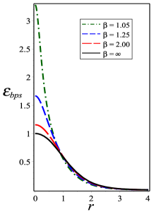
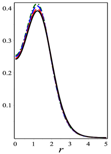
Figure 8: BPS energy density $\varepsilon_{bps}(r)$, for $n=1$. Left figure represents the $|\phi|^{4}$-model defined by Eq. (56) and right figure represents the $|\phi|^{6}$-model defined in Eq. (57).

Hereafter, we depict the profiles for the second and third models by fixing $n=1$ and some values of $\beta$. From Figs. 5 and 6 we see that for $\left|\phi\right|^{4}$-BIMH model the thickness of the vortex increases as $\beta$ decreases, i.e., when the nonlinear effects of the Born-Infeld contribution grow stronger, while for the $\left|\phi\right|^{6}$-BIMH model the new effects play a very little role, leaving almost unmodified the vortex profile. For the $\left|\phi\right|^{4}$-BIMH model this implies large modifications on the magnetic field and energy density profiles, since their maximum at $r=0$ grows quickly with $1/\beta$. On the other hand, as one could have expected, the tiny modifications on the vortex profile with $\beta$ in the $\left|\phi\right|^{6}$-BIMH model also have little effect on the magnetic field and energy density profiles. For this model these profiles have a different behavior as in the $\left|\phi\right|^{4}$-BIMH model, since their maxima are not attained at $r=0$, but rather at a finite distance, a feature that holds for any value of $\beta$.

This analysis shows that the modified-BIHM models through $\beta$ corrections do not change the qualitative features of the physical magnitudes characterizing the vortex, but are able to introduce quantitative modifications, which can become large, as in the $\left|\phi\right|^{4}$-BIMH model.

IV Conclusions

In this work we have studied a family of generalized Born-Infeld theories with a free parameter, $\beta$, and three generalizing functions which are nonnegative. These generalizing functions are constrained by the condition (32) which is the Ampere law of the model. We have worked out the theory and obtained BPS solutions of vortex-type using Bogomol’nyi trick and determined the physical properties of the solutions in terms of the magnetic flux and energy density. It was shown that whenever the conditions (25) are satisfied, the energy of the topological vortices has a lower bound

$$E\geq 2\pi v^{2}\left|n\right|,$$ (58)

which is saturated by the self-dual or BPS topological solutions. In the numerical analysis we have employed two classes of models characterized by the potential term, namely, $|\phi|^{4}$ and $|\phi|^{6}$ models, and depicted the corresponding results for the field profiles and the physical magnitudes characterizing the vortices. Such results have been compared to those of the standard Maxwell-Higgs, Chern-Simons-Higgs and Born-Infeld-Maxwell-Higgs models.

As observed in other cases of Born-Infeld-type modifications in the literature, the introduction of finite values for the Born-Infeld $\beta$ has a non-trivial impact on the field profiles of the vortices, with the result that the corresponding physical properties can be controlled by adequate combination of Born-Infeld modification and $\omega(g)$ and $G(g)$ functions. When we vary $\beta$, however, the size of the variation of the vortex properties largely depends on the model chosen, with the $|\phi|^{4}$ one showing important variation, while the $|\phi|^{6}$-one is almost insensitive to changes in $\beta$. Since topological defects find applications to many context of modern physics as useful tools for the modelling of different kinds of systems, to be able to modify the physical properties of vortex solutions is a strong motivation in favour of consideration of this kind of models. Finally let us mention that the parameter $\beta$ can not be made arbitrarily small. Our numerical analysis shows that for all $|\phi|^{4}$-models the solutions are obtained when $\beta>1$. In the case of the $|\phi|^{6}$-models it was observed that when $\beta\geq 1$ the numeric computations are always valid. The presence of a critical minimum value, $\beta_{c}$, below which numerical computations break down and no solution can be attained, seems to be a quite general phenomenon occurring in Born-Infeld type modifications, as found in other investigations in the literature Hora_Rubiera ; Moreno ; Bri . In those cases, around $\beta_{c}$ the physical magnitudes characterizing the topological defect change abruptly as $\beta$ is slowly varied, as happens in our case. Though some research has been performed about the implications of this feature, this issue remains unsolved. To conclude, we point out that the results presented here could be generalized to include non-symmetric BPS fields.

References

- (1) B. Born and L. Infeld, Proc. Roy. Soc. A 144, 425 (1935); P. A. M. Dirac, Proc. Roy. Soc. A 268, 57 (1962).
- (2) G. W. Gibbons and D. A. Rasheed, Nucl. Phys. B 454, 185 (1995).
- (3) G. Boillat, J. Math. Phys. 11, 941 (1970); G. W. Gibbons, Nucl. Phys. B 514, 603 (1998).
- (4) A. Garcia, H. Salazar, and J. F. Plebanski, Nuovo. Cim. 84, 65 (1984); M. Demianski, Found. of Phys. 16, 187 (1986); S. Fernando and D. Krug, Gen. Rel. Grav. 35, 129 (2003); T. K. Dey, Phys. Lett. B 595, 484 (2004); O. Miskovic and R. Olea, Phys. Rev. D 77, 124048 (2008).
- (5) E. Fradkin and A. A. Tseytlin, Phys. Lett. B 163, 123 (1985).
- (6) D. Brecher, Phys. Lett. B 442, 117 (1998).
- (7) A. A. Tseytlin, Nucl. Phys. B 501, 41 (1997).
- (8) A. A. Abrikosov, Zh. Eksp. Teor. Fiz. 32, 1442 (1957) [Sov. Phys. JETP 5, 1174 (1957)].
- (9) V. L. Ginzburg and L. D. Landau, Zh. Eksp. Teor. Fiz. 20, 1064 (1950). This paper was published in English in the volume: L. D. Landau, Collected Papers (Pergamon Press, Oxford, 1965), p. 546.
- (10) H. Nielsen and P. Olesen, Nucl. Phys. B 61, 1064 (1973).
-
(11)
S. Deser, R. Jackiw, and S. Templeton, Ann. Phys. (NY) 140, 372 (1982);
G. V. Dunne, arXiv:hep-th/9902115. - (12) R. Jackiw and E. J. Weinberg, Phys. Rev. Lett. 64, 2234 (1990); R. Jackiw, K. Lee, and E. J. Weinberg, Phys. Rev. D 42, 3488 (1990); J. Hong, Y. Kim, P. Y. Pac, Phys. Rev. Lett. 64, 2230 (1990); G. V. Dunne, Self-Dual Chern-Simons Theories (Springer, Heidelberg, 1995).
- (13) C. K. Lee and K. M. Lee, H. Min, Phys. Lett. B 252, 79 (1990).
- (14) S. Bolognesi and S. B. Gudnason, Nucl. Phys. B 805, 104 (2008).
- (15) D. Bazeia, E. da Hora, C. dos Santos, and R. Menezes, Phys. Rev. D 81, 125014 (2010); D. Bazeia, E. da Hora, R. Menezes, and H. P. de Oliveira, C. dos Santos, Phys. Rev. D 81, 125016 (2010); C. dos Santos and E. da Hora, Eur. Phys. J. C 70, 1145 (2010); C. dos Santos and E. da Hora, Eur. Phys. J. C 71, 1519 (2011); C. dos Santos, Phys. Rev. D 82, 125009 (2010); C. dos Santos, D. Rubiera-Garcia, J. Phys. A 44 (2011) 425402; C. Adam, L. A. Ferreira, E. da Hora, A. Wereszczynski, and W. J. Zakrzewski, J. High Energy Phys. 1308, 062 (2013).
- (16) D. Bazeia, E. da Hora, and D. Rubiera-Garcia, Phys. Rev. D 84, 125005 (2011).
- (17) G. H. Derrick, J. Math. Phys. 5, 1252 (1964).
- (18) R. Rajaraman, Solitons and Instantons (North-Holland, 1982); N. Manton, P. Sutcliffe, Topological solitons (Cambridge University Press, 2004).
- (19) E. Babichev, Phys. Rev. D 74, 085004 (2006); E. Babichev, Phys. Rev. D 77, 065021 (2008); C. Adam, N. Grandi, J. Sanchez-Guillen, and A. Wereszczynski, J. Phys. A 41, 212004 (2008); C. Adam, J. Sanchez-Guillen, and A. Wereszczynski, J. Phys. A 40, 13625 (2007); C. Adam, J. Sanchez-Guillen, and A. Wereszczynski, Phys. Rev. D 82, 085015 (2010); C. Adam, N. Grandi, P. Klimas, J. Sanchez-Guillen, and A. Wereszczynski, J. Phys. A 41, 375401 (2008); C. Adam, P. Klimas, J. Sanchez-Guillen, and A. Wereszczynski, J. Phys. A 42, 35401 (2009); M. Andrews, M. Lewandowski, M. Trodden, and D. Wesley, Phys. Rev. D 82, 105006 (2010); C. Adam, J. M. Queiruga, J. Sanchez-Guillen, and A. Wereszczynski, Phys. Rev. D 84, 025008 (2011); C. Adam, J. M. Queiruga, J. Sanchez-Guillen, and A. Wereszczynski, Phys. Rev. D 84, 065032 (2011); P. P. Avelino, D. Bazeia, and R. Menezes, Eur. Phys. J. C 71, 1683 (2011); D. Bazeia, J. D. Dantas, A. R. Gomes, L. Losano, and R. Menezes, Phys. Rev. D 84, 045010 (2011); D. Bazeia and R. Menezes, Phys. Rev. D 84, 105018 (2011); C. Adam and J. M. Queiruga, Phys. Rev. D 84, 105028 (2011); C. Adam and J. M. Queiruga, Phys. Rev. D 85, 025019 (2012); C. Adam, C. Naya, J. Sanchez-Guillen, and A. Wereszczynski, Phys. Rev. D 86, 085001 (2012); C. Adam, C. Naya, J. Sanchez-Guillen, and A. Wereszczynski, Phys. Rev. D 86, 045015 (2012); D. Bazeia, E. da Hora, and R. Menezes, Phys. Rev. D 85, 045005 (2012); D. Bazeia, A. S. Lobão Jr., and R. Menezes, Phys. Rev. D 86, 125021 (2012).
- (20) R. Casana, M. M. Ferreira, E. da Hora, and C. dos Santos, Phys. Lett. B 722, 193 (2013).
- (21) R. Casana, M. M. Ferreira, E. da Hora, and C. dos Santos, Adv. High Energy Phys. 2014, 210929 (2014).
- (22) C. Armendariz-Picon, T. Damour, and V. Mukhanov, Phys. Lett. B 458, 209 (1999).
- (23) E. Babichev, V. Mukhanov, and A. Vikman, J. High Energy Phys. 02, 101 (2008).
- (24) V. Mukhanov and A. Vikman, J. Cosmol. Astropart. Phys. 02, 004 (2005).
- (25) A. Sen, J. High Energy Phys. 07, 065 (2002).
- (26) C. Armendariz-Picon and E. A. Lim, J. Cosmol. Astropart. Phys. 08, 007 (2005).
- (27) J. Garriga and V. Mukhanov, Phys. Lett. B 458, 219 (1999); R. J. Scherrer, Phys. Rev. Lett. 93, 011301 (2004); A. D. Rendall, Classical Quantum Gravity 23, 1557 (2006).
- (28) D. Bazeia, E. da Hora, C. dos Santos, and R. Menezes, Eur. Phys. J. C 71, 1833 (2011).
- (29) D. Bazeia, E. da Hora, C. dos Santos, and R. Menezes, Phys. Rev. D 81, 125014 (2010).
- (30) D. Bazeia, R. Casana, E. da Hora, and R. Menezes, Phys. Rev. D 85, 125028 (2012).
- (31) K. Shiraishi and S. Hirenzaki, Int. J. Mod. Phys. A 6, 2635 (1991).
- (32) E. B. Bogomolny, Sov. J. Nucl. Phys. 24, 449 (1976).
- (33) E. Moreno, C. Nunez, and F. A. Schaposnik, Phys. Rev. D 58, 025015 (1998).
- (34) Y. Brihaye and B. Mercier, Phys. Rev. D 64, 044001 (2001).