1 Introduction
In this paper, we study the transmission system with
a viscoelastic term and a delay term
{ u t t ( x , t ) − a u x x ( x , t ) + ∫ 0 t g ( t − s ) u x x ( x , s ) d s + μ 1 u t ( x , t ) + μ 2 u t ( x , t − τ ) = 0 , ( x , t ) ∈ Ω × ( 0 , + ∞ ) , v t t ( x , t ) − b v x x ( x , t ) = 0 , ( x , t ) ∈ ( L 1 , L 2 ) × ( 0 , + ∞ ) , cases subscript 𝑢 𝑡 𝑡 𝑥 𝑡 𝑎 subscript 𝑢 𝑥 𝑥 𝑥 𝑡 superscript subscript 0 𝑡 𝑔 𝑡 𝑠 subscript 𝑢 𝑥 𝑥 𝑥 𝑠 differential-d 𝑠 missing-subexpression subscript 𝜇 1 subscript 𝑢 𝑡 𝑥 𝑡 subscript 𝜇 2 subscript 𝑢 𝑡 𝑥 𝑡 𝜏 0 𝑥 𝑡 Ω 0 subscript 𝑣 𝑡 𝑡 𝑥 𝑡 𝑏 subscript 𝑣 𝑥 𝑥 𝑥 𝑡 0 𝑥 𝑡 subscript 𝐿 1 subscript 𝐿 2 0 \displaystyle\left\{\begin{array}[]{ll}\displaystyle u_{tt}(x,t)-au_{xx}(x,t)+\int_{0}^{t}g(t-s)u_{xx}(x,s){\rm d}s\\
\vskip 6.0pt plus 2.0pt minus 2.0pt\displaystyle\quad\quad\quad\quad\quad\quad\quad\quad\quad+\mu_{1}u_{t}(x,t)+\mu_{2}u_{t}(x,t-\tau)=0,&(x,t)\in\Omega\times(0,+\infty),\vskip 6.0pt plus 2.0pt minus 2.0pt\\
\displaystyle v_{tt}(x,t)-bv_{xx}(x,t)=0,&(x,t)\in(L_{1},L_{2})\times(0,+\infty),\end{array}\right. (1.4)
under the boundary and transmission conditions
{ u ( 0 , t ) = u ( L 3 , t ) = 0 , u ( L i , t ) = v ( L i , t ) , i = 1 , 2 , ( a − ∫ 0 t g ( s ) d s ) u x ( L i , t ) = b v x ( L i , t ) , i = 1 , 2 , cases 𝑢 0 𝑡 𝑢 subscript 𝐿 3 𝑡 0 missing-subexpression 𝑢 subscript 𝐿 𝑖 𝑡 𝑣 subscript 𝐿 𝑖 𝑡 𝑖 1 2
𝑎 superscript subscript 0 𝑡 𝑔 𝑠 differential-d 𝑠 subscript 𝑢 𝑥 subscript 𝐿 𝑖 𝑡 𝑏 subscript 𝑣 𝑥 subscript 𝐿 𝑖 𝑡 𝑖 1 2
\displaystyle\left\{\begin{array}[]{ll}\displaystyle u(0,t)=u(L_{3},t)=0,\vskip 6.0pt plus 2.0pt minus 2.0pt\\
\vskip 6.0pt plus 2.0pt minus 2.0pt\displaystyle u(L_{i},t)=v(L_{i},t),&i=1,2,\vskip 6.0pt plus 2.0pt minus 2.0pt\\
\displaystyle\left(a-\int_{0}^{t}g(s){\rm d}s\right)u_{x}(L_{i},t)=bv_{x}(L_{i},t),&i=1,2,\end{array}\right. (1.8)
and the initial conditions
{ u ( x , 0 ) = u 0 ( x ) , u t ( x , 0 ) = u 1 ( x ) , x ∈ Ω , u t ( x , t − τ ) = f 0 ( x , t − τ ) , x ∈ Ω , t ∈ [ 0 , τ ] , v ( x , 0 ) = v 0 ( x ) , v t ( x , 0 ) = v 1 ( x ) , x ∈ ( L 1 , L 2 ) , cases formulae-sequence 𝑢 𝑥 0 subscript 𝑢 0 𝑥 subscript 𝑢 𝑡 𝑥 0 subscript 𝑢 1 𝑥 𝑥 Ω subscript 𝑢 𝑡 𝑥 𝑡 𝜏 subscript 𝑓 0 𝑥 𝑡 𝜏 formulae-sequence 𝑥 Ω 𝑡 0 𝜏 formulae-sequence 𝑣 𝑥 0 subscript 𝑣 0 𝑥 subscript 𝑣 𝑡 𝑥 0 subscript 𝑣 1 𝑥 𝑥 subscript 𝐿 1 subscript 𝐿 2 \displaystyle\left\{\begin{array}[]{ll}\displaystyle u(x,0)=u_{0}(x),\quad u_{t}(x,0)=u_{1}(x),&x\in\Omega,\vskip 6.0pt plus 2.0pt minus 2.0pt\\
\vskip 6.0pt plus 2.0pt minus 2.0pt\displaystyle u_{t}(x,t-\tau)=f_{0}(x,t-\tau),&x\in\Omega,\quad t\in[0,\tau],\vskip 6.0pt plus 2.0pt minus 2.0pt\\
\displaystyle v(x,0)=v_{0}(x),\quad v_{t}(x,0)=v_{1}(x),&x\in(L_{1},L_{2}),\end{array}\right. (1.12)
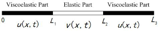
where 0 < L 1 < L 2 < L 3 0 subscript 𝐿 1 subscript 𝐿 2 subscript 𝐿 3 0<L_{1}<L_{2}<L_{3} Ω = ( 0 , L 1 ) ∪ ( L 2 , L 3 ) Ω 0 subscript 𝐿 1 subscript 𝐿 2 subscript 𝐿 3 \Omega=(0,L_{1})\cup(L_{2},L_{3}) a 𝑎 a b 𝑏 b μ 1 subscript 𝜇 1 \mu_{1} μ 2 subscript 𝜇 2 \mu_{2} τ > 0 𝜏 0 \tau>0
Figure 1: The configuration.
The problems like (1.4 1.12
In recent years, many authors have investigated wave equations with viscoelastic damping and showed that the dissipation produced by the viscoelastic part can produce the decay of the solution, see [5 , 6 , 7 , 8 , 10 , 14 , 15 , 16 , 18 , 22 , 23 , 24 ] and the references therein. For example,
Cavalcanti et al. [8 ] studied the following equation:
u t t − Δ u + ∫ 0 t g ( t − τ ) Δ u ( τ ) d τ + a ( x ) u t + | u | γ u = 0 , in Ω × ( 0 , ∞ ) , subscript 𝑢 𝑡 𝑡 Δ 𝑢 superscript subscript 0 𝑡 𝑔 𝑡 𝜏 Δ 𝑢 𝜏 differential-d 𝜏 𝑎 𝑥 subscript 𝑢 𝑡 superscript 𝑢 𝛾 𝑢 0 in Ω 0
u_{tt}-\Delta u+\int_{0}^{t}g(t-\tau)\Delta u(\tau){\rm d}\tau+a(x)u_{t}+|u|^{\gamma}u=0,\quad{\rm in}\quad\Omega\times(0,\infty),
where a : Ω → ℝ + : 𝑎 → Ω subscript ℝ a:\Omega\rightarrow\mathbb{R}_{+} a ( x ) ≥ a 0 > 0 𝑎 𝑥 subscript 𝑎 0 0 a(x)\geq a_{0}>0 ω ⊂ Ω 𝜔 Ω \omega\subset\Omega ω 𝜔 \omega
− ξ 1 g ( t ) ≤ g ′ ( t ) ≤ − ξ 2 g ( t ) , t ≥ 0 , formulae-sequence subscript 𝜉 1 𝑔 𝑡 superscript 𝑔 ′ 𝑡 subscript 𝜉 2 𝑔 𝑡 𝑡 0 -\xi_{1}g(t)\leq g^{\prime}(t)\leq-\xi_{2}g(t),\quad t\geq 0,
the authors showed the exponential decay. Then Berrimi and Messaoudi [5 ] proved the same
result under weaker conditions on both a 𝑎 a g 𝑔 g [6 ] considered the equation
u t t − Δ u + ∫ 0 t g ( t − τ ) Δ u ( τ ) d τ = | u | γ u , in Ω × ( 0 , ∞ ) , subscript 𝑢 𝑡 𝑡 Δ 𝑢 superscript subscript 0 𝑡 𝑔 𝑡 𝜏 Δ 𝑢 𝜏 differential-d 𝜏 superscript 𝑢 𝛾 𝑢 in Ω 0
u_{tt}-\Delta u+\int_{0}^{t}g(t-\tau)\Delta u(\tau){\rm d}\tau=|u|^{\gamma}u,\quad{\rm in}\quad\Omega\times(0,\infty),
with only the viscoelastic dissipation and proved
that the solution energy decays
exponentially or polynomially depending on the rate of the decay of the relaxation function g 𝑔 g [18 ] investigated the following viscoelastic equation:
u t t − Δ u + ∫ 0 t g ( t − τ ) Δ u ( τ ) d τ = 0 , in Ω × ( 0 , ∞ ) , subscript 𝑢 𝑡 𝑡 Δ 𝑢 superscript subscript 0 𝑡 𝑔 𝑡 𝜏 Δ 𝑢 𝜏 differential-d 𝜏 0 in Ω 0
u_{tt}-\Delta u+\int_{0}^{t}g(t-\tau)\Delta u(\tau){\rm d}\tau=0,\quad{\rm in}\quad\Omega\times(0,\infty),
in a bounded domain, and established a more
general decay result, from which the usual exponential and polynomial decay rates
are only special cases.
Afterwards, Han and Wang [10 ] studied the nonlinear viscoelastic equation
u t t − Δ u + ∫ 0 t g ( t − τ ) Δ u ( τ ) d τ + | u | k ∂ j ( u t ) = | u | p − 1 u , in Ω × ( 0 , T ) . subscript 𝑢 𝑡 𝑡 Δ 𝑢 superscript subscript 0 𝑡 𝑔 𝑡 𝜏 Δ 𝑢 𝜏 differential-d 𝜏 superscript 𝑢 𝑘 𝑗 subscript 𝑢 𝑡 superscript 𝑢 𝑝 1 𝑢 in Ω 0 𝑇
u_{tt}-\Delta u+\int_{0}^{t}g(t-\tau)\Delta u(\tau){\rm d}\tau+|u|^{k}\partial j(u_{t})=|u|^{p-1}u,\quad{\rm in}\quad\Omega\times(0,T).
They obtained the global existence of generalized solutions, weak solutions for
the equation. In addition, the finite time blow-up of weak solutions is established provided that the initial energy is negative
and the exponent p 𝑝 p
It is well known that delay effects, which arise in many practical problems, may be sources of instability.
Hence, the control of PDEs with time delay effects has become an active area of research in recent years.
For example, it was proved in
[9 , 20 ] that an arbitrarily small delay may destabilize
a system which is uniformly asymptotically stable in the absence of delay unless
additional conditions or control terms were used.
A boundary stabilization problem for the wave equation with interior delay studied in [1 ] . The authors proved an exponential stability result under some Lions geometric condition.
Kirane and Said-Houari [11 ] considered the viscoelastic wave equation with a delay
u t t ( x , t ) − Δ u ( x , t ) + ∫ 0 t g ( t − s ) Δ u ( x , t − s ) d s + μ 1 u t ( x , t ) + μ 2 u t ( x , t − τ ) = 0 , in Ω × ( 0 , ∞ ) , subscript 𝑢 𝑡 𝑡 𝑥 𝑡 Δ 𝑢 𝑥 𝑡 superscript subscript 0 𝑡 𝑔 𝑡 𝑠 Δ 𝑢 𝑥 𝑡 𝑠 differential-d 𝑠 subscript 𝜇 1 subscript 𝑢 𝑡 𝑥 𝑡 subscript 𝜇 2 subscript 𝑢 𝑡 𝑥 𝑡 𝜏 0 in Ω 0
u_{tt}(x,t)-\Delta u(x,t)+\int_{0}^{t}g(t-s)\Delta u(x,t-s){\rm d}s+\mu_{1}u_{t}(x,t)+\mu_{2}u_{t}(x,t-\tau)=0,\quad{\rm in}\quad\Omega\times(0,\infty),
where μ 1 subscript 𝜇 1 \mu_{1} μ 2 subscript 𝜇 2 \mu_{2} 0 ≤ μ 2 ≤ μ 1 0 subscript 𝜇 2 subscript 𝜇 1 0\leq\mu_{2}\leq\mu_{1} [13 ] improved this result by considering the equation with a time-varying delay term, with not necessarily positive coefficient μ 2 subscript 𝜇 2 \mu_{2}
Transmission problems
related to (1.4 1.12 [4 ]
investigated the transmission problem with frictional damping
and showed the well-posedness and exponential stability of the total energy.
Muñoz Rivera and
Portillo Oquendo [19 ] considered the transmission problem of viscoelastic waves
and proved that the dissipation produced by the viscoelastic part can produce exponential decay
of the solution, no matter how small its size is.
Bae [3 ] studied the transmission problem,
in which one component is clamped and the other is in a viscoelastic
fluid producing a dissipative mechanism on the boundary, and established a decay result
which depends on the rate of the decay of the relaxation function.
Motivated by the above results, we intend to consider the well-posedness and the general decay result of
problem (1.4 1.12 1.4 1.12
The paper is organized as follows. In Section 2 3 4
2 Preliminaries and main results
In this section, we present some materials that shall be used in order to prove our main results.
Let us first introduce the following notations:
( g ∗ h ) ( t ) := ∫ 0 t g ( t − s ) h ( s ) d s , assign 𝑔 ℎ 𝑡 superscript subscript 0 𝑡 𝑔 𝑡 𝑠 ℎ 𝑠 differential-d 𝑠 \displaystyle(g*h)(t):=\int_{0}^{t}g(t-s)h(s){\rm d}s,
( g ⋄ h ) ( t ) := ∫ 0 t g ( t − s ) | h ( t ) − h ( s ) | d s , assign ⋄ 𝑔 ℎ 𝑡 superscript subscript 0 𝑡 𝑔 𝑡 𝑠 ℎ 𝑡 ℎ 𝑠 differential-d 𝑠 \displaystyle(g\diamond h)(t):=\int_{0}^{t}g(t-s)|h(t)-h(s)|{\rm d}s,
( g □ h ) ( t ) := ∫ 0 t g ( t − s ) | h ( t ) − h ( s ) | 2 d s . assign 𝑔 □ ℎ 𝑡 superscript subscript 0 𝑡 𝑔 𝑡 𝑠 superscript ℎ 𝑡 ℎ 𝑠 2 differential-d 𝑠 \displaystyle(g\square h)(t):=\int_{0}^{t}g(t-s)|h(t)-h(s)|^{2}{\rm d}s.
Note that the sign of ( g □ h ) ( t ) 𝑔 □ ℎ 𝑡 (g\square h)(t) g 𝑔 g
( g ∗ h ) ( t ) = ( ∫ 0 t g ( s ) d s ) h ( t ) − ( g ⋄ h ) ( t ) , 𝑔 ℎ 𝑡 superscript subscript 0 𝑡 𝑔 𝑠 differential-d 𝑠 ℎ 𝑡 ⋄ 𝑔 ℎ 𝑡 \displaystyle(g*h)(t)=\left(\int_{0}^{t}g(s){\rm d}s\right)h(t)-(g\diamond h)(t),
| ( g ⋄ h ) ( t ) | 2 ≤ ( ∫ 0 t | g ( s ) | d s ) ( | g | □ h ) ( t ) . superscript ⋄ 𝑔 ℎ 𝑡 2 superscript subscript 0 𝑡 𝑔 𝑠 differential-d 𝑠 𝑔 □ ℎ 𝑡 \displaystyle|(g\diamond h)(t)|^{2}\leq\left(\int_{0}^{t}|g(s)|{\rm d}s\right)(|g|\square h)(t).
Lemma 2.1
For any g , h ∈ C 1 ( ℝ ) 𝑔 ℎ
superscript 𝐶 1 ℝ g,h\in C^{1}(\mathbb{R})
2 [ g ∗ h ] h ′ = g ′ □ h − g ( t ) | h | 2 − d d t { g □ h − ( ∫ 0 t g ( s ) d s ) | h | 2 } . 2 delimited-[] 𝑔 ℎ superscript ℎ ′ superscript 𝑔 ′ □ ℎ 𝑔 𝑡 superscript ℎ 2 𝑑 𝑑 𝑡 𝑔 □ ℎ superscript subscript 0 𝑡 𝑔 𝑠 differential-d 𝑠 superscript ℎ 2 2[g*h]h^{\prime}=g^{\prime}\square h-g(t)|h|^{2}-\frac{d}{dt}\left\{g\square h-\left(\int_{0}^{t}g(s){\rm d}s\right)|h|^{2}\right\}.
For the relaxation function g 𝑔 g
(G1) g 𝑔 g ℝ + → ℝ + → subscript ℝ subscript ℝ \mathbb{R}_{+}\rightarrow\mathbb{R}_{+} C 1 superscript 𝐶 1 C^{1}
g ( 0 ) > 0 , 0 < β ( t ) := a − ∫ 0 t g ( s ) d s and 0 < β 0 := a − ∫ 0 ∞ g ( s ) d s . formulae-sequence formulae-sequence 𝑔 0 0 0 𝛽 𝑡 assign 𝑎 superscript subscript 0 𝑡 𝑔 𝑠 differential-d 𝑠 and 0
subscript 𝛽 0 assign 𝑎 superscript subscript 0 𝑔 𝑠 differential-d 𝑠 g(0)>0,\quad 0<\beta(t):=a-\int_{0}^{t}g(s){\rm d}s\quad{\rm and}\quad 0<\beta_{0}:=a-\int_{0}^{\infty}g(s){\rm d}s.
(G2) There exists a nonincreasing differentiable function ξ ( t ) 𝜉 𝑡 \xi(t) ℝ + → ℝ + → subscript ℝ subscript ℝ \mathbb{R}_{+}\rightarrow\mathbb{R}_{+}
g ′ ( t ) ≤ − ξ ( t ) g ( t ) , ∀ t ≥ 0 and ∫ 0 ∞ ξ ( t ) d t = + ∞ . formulae-sequence superscript 𝑔 ′ 𝑡 𝜉 𝑡 𝑔 𝑡 formulae-sequence for-all 𝑡 0 and
superscript subscript 0 𝜉 𝑡 differential-d 𝑡 g^{\prime}(t)\leq-\xi(t)g(t),\quad\forall t\geq 0\quad{\rm and}\quad\int_{0}^{\infty}\xi(t){\rm d}t=+\infty.
These hypotheses imply that
β 0 ≤ β ( t ) ≤ a . subscript 𝛽 0 𝛽 𝑡 𝑎 \beta_{0}\leq\beta(t)\leq a. (2.1)
As in [20 ] , we introduce the following variable:
z ( x , ρ , t ) = u t ( x , t − τ ρ ) , ( x , ρ , t ) ∈ Ω × ( 0 , 1 ) × ( 0 , ∞ ) . formulae-sequence 𝑧 𝑥 𝜌 𝑡 subscript 𝑢 𝑡 𝑥 𝑡 𝜏 𝜌 𝑥 𝜌 𝑡 Ω 0 1 0 z(x,\rho,t)=u_{t}(x,t-\tau\rho),\quad(x,\rho,t)\in\Omega\times(0,1)\times(0,\infty).
Then the above variable z 𝑧 z
τ z t ( x , ρ , t ) + z ρ ( x , ρ , t ) = 0 , ( x , ρ , t ) ∈ Ω × ( 0 , 1 ) × ( 0 , ∞ ) . formulae-sequence 𝜏 subscript 𝑧 𝑡 𝑥 𝜌 𝑡 subscript 𝑧 𝜌 𝑥 𝜌 𝑡 0 𝑥 𝜌 𝑡 Ω 0 1 0 \tau z_{t}(x,\rho,t)+z_{\rho}(x,\rho,t)=0,\quad(x,\rho,t)\in\Omega\times(0,1)\times(0,\infty). (2.2)
Thus, system (1.4
{ u t t ( x , t ) − a u x x ( x , t ) + g ∗ u x x + μ 1 u t ( x , t ) + μ 2 z ( x , 1 , t ) = 0 , ( x , t ) ∈ Ω × ( 0 , + ∞ ) , v t t ( x , t ) − b v x x ( x , t ) = 0 , ( x , t ) ∈ ( L 1 , L 2 ) × ( 0 , + ∞ ) , τ z t ( x , ρ , t ) + z ρ ( x , ρ , t ) = 0 , ( x , ρ , t ) ∈ Ω × ( 0 , 1 ) × ( 0 , + ∞ ) , cases subscript 𝑢 𝑡 𝑡 𝑥 𝑡 𝑎 subscript 𝑢 𝑥 𝑥 𝑥 𝑡 𝑔 subscript 𝑢 𝑥 𝑥 missing-subexpression subscript 𝜇 1 subscript 𝑢 𝑡 𝑥 𝑡 subscript 𝜇 2 𝑧 𝑥 1 𝑡 0 𝑥 𝑡 Ω 0 subscript 𝑣 𝑡 𝑡 𝑥 𝑡 𝑏 subscript 𝑣 𝑥 𝑥 𝑥 𝑡 0 𝑥 𝑡 subscript 𝐿 1 subscript 𝐿 2 0 𝜏 subscript 𝑧 𝑡 𝑥 𝜌 𝑡 subscript 𝑧 𝜌 𝑥 𝜌 𝑡 0 𝑥 𝜌 𝑡 Ω 0 1 0 \displaystyle\left\{\begin{array}[]{ll}\displaystyle u_{tt}(x,t)-au_{xx}(x,t)+g*u_{xx}\\
\vskip 6.0pt plus 2.0pt minus 2.0pt\displaystyle\quad\quad\quad\quad\quad\quad\quad\quad\quad+\mu_{1}u_{t}(x,t)+\mu_{2}z(x,1,t)=0,&(x,t)\in\Omega\times(0,+\infty),\\
\displaystyle v_{tt}(x,t)-bv_{xx}(x,t)=0,&(x,t)\in(L_{1},L_{2})\times(0,+\infty),\vskip 6.0pt plus 2.0pt minus 2.0pt\\
\displaystyle\tau z_{t}(x,\rho,t)+z_{\rho}(x,\rho,t)=0,&(x,\rho,t)\in\Omega\times(0,1)\times(0,+\infty),\end{array}\right. (2.7)
and the boundary and transmission conditions (1.8
{ u ( 0 , t ) = u ( L 3 , t ) = 0 , u ( L i , t ) = v ( L i , t ) , i = 1 , 2 , t ∈ ( 0 , + ∞ ) , ( a − ∫ 0 t g ( s ) d s ) u x ( L i , t ) = b v x ( L i , t ) , i = 1 , 2 , t ∈ ( 0 , + ∞ ) , z ( x , 0 , t ) = u t ( x , t ) , ( x , t ) ∈ Ω × ( 0 , + ∞ ) , z ( x , 1 , t ) = f 0 ( x , t − τ ) , ( x , t ) ∈ Ω × ( 0 , τ ) . cases 𝑢 0 𝑡 𝑢 subscript 𝐿 3 𝑡 0 missing-subexpression formulae-sequence 𝑢 subscript 𝐿 𝑖 𝑡 𝑣 subscript 𝐿 𝑖 𝑡 𝑖 1 2
𝑡 0 formulae-sequence 𝑎 superscript subscript 0 𝑡 𝑔 𝑠 differential-d 𝑠 subscript 𝑢 𝑥 subscript 𝐿 𝑖 𝑡 𝑏 subscript 𝑣 𝑥 subscript 𝐿 𝑖 𝑡 𝑖 1 2
𝑡 0 𝑧 𝑥 0 𝑡 subscript 𝑢 𝑡 𝑥 𝑡 𝑥 𝑡 Ω 0 𝑧 𝑥 1 𝑡 subscript 𝑓 0 𝑥 𝑡 𝜏 𝑥 𝑡 Ω 0 𝜏 \displaystyle\left\{\begin{array}[]{ll}\displaystyle u(0,t)=u(L_{3},t)=0,\vskip 6.0pt plus 2.0pt minus 2.0pt\\
\vskip 6.0pt plus 2.0pt minus 2.0pt\displaystyle u(L_{i},t)=v(L_{i},t),\quad\quad\quad\quad\quad\quad\quad\quad\quad\quad i=1,2,&t\in(0,+\infty),\vskip 6.0pt plus 2.0pt minus 2.0pt\\
\vskip 6.0pt plus 2.0pt minus 2.0pt\displaystyle\left(a-\int_{0}^{t}g(s){\rm d}s\right)u_{x}(L_{i},t)=bv_{x}(L_{i},t),\quad i=1,2,&t\in(0,+\infty),\vskip 6.0pt plus 2.0pt minus 2.0pt\\
\vskip 6.0pt plus 2.0pt minus 2.0pt\displaystyle z(x,0,t)=u_{t}(x,t),&(x,t)\in\Omega\times(0,+\infty),\vskip 6.0pt plus 2.0pt minus 2.0pt\\
\displaystyle z(x,1,t)=f_{0}(x,t-\tau),&(x,t)\in\Omega\times(0,\tau).\end{array}\right. (2.13)
Similar to [21 ] , we denote the Hilbert spaces
𝒱 = { \displaystyle\mathcal{V}=\bigg{\{} ( u , v ) ∈ H 1 ( Ω ) ∩ H 1 ( L 1 , L 2 ) : u ( 0 , t ) = u ( L 3 , 0 ) = 0 , u ( L i , t ) = v ( L i , t ) , . \displaystyle(u,v)\in H^{1}(\Omega)\cap H^{1}(L_{1},L_{2}):u(0,t)=u(L_{3},0)=0,u(L_{i},t)=v(L_{i},t),\bigg{.}
. ( a − ∫ 0 t g ( s ) d s ) u x ( L i , t ) = b v x ( L i , t ) , i = 1 , 2 } \displaystyle\bigg{.}\left(a-\int_{0}^{t}g(s){\rm d}s\right)u_{x}(L_{i},t)=bv_{x}(L_{i},t),i=1,2\bigg{\}}
and
ℒ 2 = L 2 ( Ω ) × L 2 ( L 1 , L 2 ) . superscript ℒ 2 superscript 𝐿 2 Ω superscript 𝐿 2 subscript 𝐿 1 subscript 𝐿 2 \mathcal{L}^{2}=L^{2}(\Omega)\times L^{2}(L_{1},L_{2}).
Then the existence result reads as follows:
Theorem 2.2
Assume that μ 2 ≤ μ 1 subscript 𝜇 2 subscript 𝜇 1 \mu_{2}\leq\mu_{1} ( G 1 ) 𝐺 1 (G1) ( G 2 ) 𝐺 2 (G2) ( u 0 , v 0 ) ∈ 𝒱 subscript 𝑢 0 subscript 𝑣 0 𝒱 (u_{0},v_{0})\in\mathcal{V} ( u 1 , v 1 ) ∈ ℒ 2 subscript 𝑢 1 subscript 𝑣 1 superscript ℒ 2 (u_{1},v_{1})\in\mathcal{L}^{2} f 0 ∈ L 2 ( ( 0 , 1 ) , H 1 ( Ω ) ) subscript 𝑓 0 superscript 𝐿 2 0 1 superscript 𝐻 1 Ω f_{0}\in L^{2}((0,1),H^{1}(\Omega)) ( u , v , z ) 𝑢 𝑣 𝑧 (u,v,z) 2.7 2.13
( u , v ) ∈ C ( 0 , ∞ ; 𝒱 ) ∩ C 1 ( 0 , ∞ ; ℒ 2 ) , 𝑢 𝑣 𝐶 0 𝒱 superscript 𝐶 1 0 superscript ℒ 2 \displaystyle(u,v)\in C(0,\infty;\mathcal{V})\cap C^{1}(0,\infty;\mathcal{L}^{2}),
z ∈ C ( 0 , ∞ ; L 2 ( ( 0 , 1 ) , H 1 ( Ω ) ) ) . 𝑧 𝐶 0 superscript 𝐿 2 0 1 superscript 𝐻 1 Ω \displaystyle z\in C(0,\infty;L^{2}((0,1),H^{1}(\Omega))).
For any regular solution
of (1.4 1.12
E ( t ) = 𝐸 𝑡 absent \displaystyle E(t)= 1 2 ∫ Ω u t 2 ( x , t ) d x + 1 2 β ( t ) ∫ Ω u x 2 ( x , t ) d x + 1 2 ∫ Ω ( g □ u x ) d x 1 2 subscript Ω superscript subscript 𝑢 𝑡 2 𝑥 𝑡 differential-d 𝑥 1 2 𝛽 𝑡 subscript Ω superscript subscript 𝑢 𝑥 2 𝑥 𝑡 differential-d 𝑥 1 2 subscript Ω 𝑔 □ subscript 𝑢 𝑥 differential-d 𝑥 \displaystyle\frac{1}{2}\int_{\Omega}u_{t}^{2}(x,t){\rm d}x+\frac{1}{2}\beta(t)\int_{\Omega}u_{x}^{2}(x,t){\rm d}x+\frac{1}{2}\int_{\Omega}(g\square u_{x}){\rm d}x
+ 1 2 ∫ L 1 L 2 [ v t 2 ( x , t ) + b v x 2 ( x , t ) ] d x + ζ 2 ∫ Ω ∫ 0 1 z 2 ( x , ρ , t ) d ρ d x , 1 2 superscript subscript subscript 𝐿 1 subscript 𝐿 2 delimited-[] superscript subscript 𝑣 𝑡 2 𝑥 𝑡 𝑏 superscript subscript 𝑣 𝑥 2 𝑥 𝑡 differential-d 𝑥 𝜁 2 subscript Ω superscript subscript 0 1 superscript 𝑧 2 𝑥 𝜌 𝑡 differential-d 𝜌 differential-d 𝑥 \displaystyle+\frac{1}{2}\int_{L_{1}}^{L_{2}}\left[v_{t}^{2}(x,t)+bv_{x}^{2}(x,t)\right]{\rm d}x+\frac{\zeta}{2}\int_{\Omega}\int_{0}^{1}z^{2}(x,\rho,t){\rm d}\rho{\rm d}x, (2.14)
where ζ 𝜁 \zeta
τ μ 2 < ζ < τ ( 2 μ 1 − μ 2 ) . 𝜏 subscript 𝜇 2 𝜁 𝜏 2 subscript 𝜇 1 subscript 𝜇 2 \tau\mu_{2}<\zeta<\tau(2\mu_{1}-\mu_{2}). (2.15)
Our decay result reads as follows:
Theorem 2.3
Let ( u , v ) 𝑢 𝑣 (u,v) 1.4 1.12 μ 2 < μ 1 subscript 𝜇 2 subscript 𝜇 1 \mu_{2}<\mu_{1} ( G 1 ) 𝐺 1 (G1) ( G 2 ) 𝐺 2 (G2)
b > 4 ( L 2 − L 1 ) L 1 + L 3 − L 2 β 0 , a > 4 ( L 2 − L 1 ) L 1 + L 3 − L 2 β 0 formulae-sequence 𝑏 4 subscript 𝐿 2 subscript 𝐿 1 subscript 𝐿 1 subscript 𝐿 3 subscript 𝐿 2 subscript 𝛽 0 𝑎 4 subscript 𝐿 2 subscript 𝐿 1 subscript 𝐿 1 subscript 𝐿 3 subscript 𝐿 2 subscript 𝛽 0 b>\frac{4(L_{2}-L_{1})}{L_{1}+L_{3}-L_{2}}\beta_{0},\quad a>\frac{4(L_{2}-L_{1})}{L_{1}+L_{3}-L_{2}}\beta_{0} (2.16)
hold,
then there exists constants γ 0 , γ 2 > 0 subscript 𝛾 0 subscript 𝛾 2
0 \gamma_{0},\gamma_{2}>0 t ∈ ℝ + 𝑡 subscript ℝ t\in\mathbb{R}_{+} γ 1 ∈ ( 0 , γ 0 ) subscript 𝛾 1 0 subscript 𝛾 0 \gamma_{1}\in(0,\gamma_{0})
E ( t ) ≤ γ 2 e − γ 1 ∫ 0 t ξ ( s ) d s . 𝐸 𝑡 subscript 𝛾 2 superscript 𝑒 subscript 𝛾 1 superscript subscript 0 𝑡 𝜉 𝑠 differential-d 𝑠 E(t)\leq\gamma_{2}e^{-\gamma_{1}\int_{0}^{t}\xi(s){\rm d}s}. (2.17)
3 Well-posedness of the problem
In this section, we will prove the existence and uniqueness of problem
(1.4 1.12
Proof of Theorem 2.2
We divide the proof of Theorem 2.2
Step 1: Faedo-Galerkin approximation.
We construct approximations of the solution ( u , v , z ) 𝑢 𝑣 𝑧 (u,v,z) n ≥ 1 𝑛 1 n\geq 1 W n = span { w 1 , … , w i } subscript 𝑊 𝑛 span subscript 𝑤 1 … subscript 𝑤 𝑖 W_{n}={\rm span}\{w_{1},\ldots,w_{i}\} H 1 ( Ω ) superscript 𝐻 1 Ω H^{1}(\Omega) Y n = span { ψ 1 , … , ψ i } subscript 𝑌 𝑛 span subscript 𝜓 1 … subscript 𝜓 𝑖 Y_{n}={\rm span}\{\psi_{1},\ldots,\psi_{i}\} H 1 ( L 1 , L 2 ) superscript 𝐻 1 subscript 𝐿 1 subscript 𝐿 2 H^{1}(L_{1},L_{2})
Now, we define for 1 ≤ j ≤ n 1 𝑗 𝑛 1\leq j\leq n φ j ( x , ρ ) subscript 𝜑 𝑗 𝑥 𝜌 \varphi_{j}(x,\rho)
φ j ( x , 0 ) = w j ( x ) . subscript 𝜑 𝑗 𝑥 0 subscript 𝑤 𝑗 𝑥 \varphi_{j}(x,0)=w_{j}(x).
Then we may extend φ j ( x , 0 ) subscript 𝜑 𝑗 𝑥 0 \varphi_{j}(x,0) φ j ( x , ρ ) subscript 𝜑 𝑗 𝑥 𝜌 \varphi_{j}(x,\rho) L 2 ( ( 0 , 1 ) , H 1 ( Ω ) ) superscript 𝐿 2 0 1 superscript 𝐻 1 Ω L^{2}((0,1),H^{1}(\Omega)) V n = span { φ 1 , … , φ n } subscript 𝑉 𝑛 span subscript 𝜑 1 … subscript 𝜑 𝑛 V_{n}={\rm span}\{\varphi_{1},\ldots,\varphi_{n}\}
We choose sequences ( u 0 ( n ) ) superscript subscript 𝑢 0 𝑛 \left(u_{0}^{(n)}\right) ( u 1 ( n ) ) superscript subscript 𝑢 1 𝑛 \left(u_{1}^{(n)}\right) W n subscript 𝑊 𝑛 W_{n} ( v 0 ( n ) ) superscript subscript 𝑣 0 𝑛 \left(v_{0}^{(n)}\right) ( v 1 ( n ) ) superscript subscript 𝑣 1 𝑛 \left(v_{1}^{(n)}\right) Y n subscript 𝑌 𝑛 Y_{n} ( z 0 ( n ) ) superscript subscript 𝑧 0 𝑛 \left(z_{0}^{(n)}\right) V n subscript 𝑉 𝑛 V_{n} u 0 ( n ) → u 0 → superscript subscript 𝑢 0 𝑛 subscript 𝑢 0 u_{0}^{(n)}\rightarrow u_{0} H 1 ( Ω ) superscript 𝐻 1 Ω H^{1}(\Omega) u 1 ( n ) → u 1 → superscript subscript 𝑢 1 𝑛 subscript 𝑢 1 u_{1}^{(n)}\rightarrow u_{1} H 1 ( Ω ) superscript 𝐻 1 Ω H^{1}(\Omega) v 0 ( n ) → v 0 → superscript subscript 𝑣 0 𝑛 subscript 𝑣 0 v_{0}^{(n)}\rightarrow v_{0} H 1 ( L 1 , L 2 ) superscript 𝐻 1 subscript 𝐿 1 subscript 𝐿 2 H^{1}(L_{1},L_{2}) v 1 ( n ) → v 1 → superscript subscript 𝑣 1 𝑛 subscript 𝑣 1 v_{1}^{(n)}\rightarrow v_{1} H 1 ( L 1 , L 2 ) superscript 𝐻 1 subscript 𝐿 1 subscript 𝐿 2 H^{1}(L_{1},L_{2}) z 0 ( n ) → f 0 → superscript subscript 𝑧 0 𝑛 subscript 𝑓 0 z_{0}^{(n)}\rightarrow f_{0} L 2 ( ( 0 , 1 ) , H 1 ( Ω ) ) superscript 𝐿 2 0 1 superscript 𝐻 1 Ω L^{2}((0,1),H^{1}(\Omega))
We define the approximations
( u ( n ) ( x , t ) , v ( n ) ( x , t ) ) = ∑ i = 1 n h i ( n ) ( t ) ( w i ( x ) , ψ i ( x ) ) and z ( n ) ( x , ρ , t ) = ∑ i = 1 n f i ( n ) ( t ) φ i ( x ) , formulae-sequence superscript 𝑢 𝑛 𝑥 𝑡 superscript 𝑣 𝑛 𝑥 𝑡 superscript subscript 𝑖 1 𝑛 superscript subscript ℎ 𝑖 𝑛 𝑡 subscript 𝑤 𝑖 𝑥 subscript 𝜓 𝑖 𝑥 and
superscript 𝑧 𝑛 𝑥 𝜌 𝑡 superscript subscript 𝑖 1 𝑛 superscript subscript 𝑓 𝑖 𝑛 𝑡 subscript 𝜑 𝑖 𝑥 \left(u^{(n)}(x,t),v^{(n)}(x,t)\right)=\sum\limits_{i=1}^{n}h_{i}^{(n)}(t)(w_{i}(x),\psi_{i}(x))\quad{\rm and}\quad z^{(n)}(x,\rho,t)=\sum\limits_{i=1}^{n}f_{i}^{(n)}(t)\varphi_{i}(x),
where ( u ( n ) ( t ) , v ( n ) ( t ) , z ( n ) ( t ) ) superscript 𝑢 𝑛 𝑡 superscript 𝑣 𝑛 𝑡 superscript 𝑧 𝑛 𝑡 \left(u^{(n)}(t),v^{(n)}(t),z^{(n)}(t)\right)
{ ∫ Ω u t t ( n ) w i d x − [ ( a u x ( n ) − g ∗ u x ( n ) ) w i ] ∂ Ω + ∫ Ω a u x ( n ) w i x d x − ∫ Ω ( g ∗ u x ( n ) ) w i x d x + ∫ Ω μ 1 u t ( n ) w i d x + ∫ Ω μ 2 z ( n ) ( x , 1 , t ) w i d x = 0 , ∫ L 1 L 2 v t t ( n ) ψ i d x + ∫ L 1 L 2 b v x ( n ) ψ i x d x − [ b v x ( n ) ψ i ] L 1 L 2 = 0 , z ( n ) ( x , 0 , t ) = u t ( n ) ( x , t ) , ( u ( n ) ( 0 ) , u t ( n ) ( 0 ) ) = ( u 0 ( n ) , u 1 ( n ) ) cases subscript Ω superscript subscript 𝑢 𝑡 𝑡 𝑛 subscript 𝑤 𝑖 differential-d 𝑥 subscript delimited-[] 𝑎 superscript subscript 𝑢 𝑥 𝑛 𝑔 superscript subscript 𝑢 𝑥 𝑛 subscript 𝑤 𝑖 Ω subscript Ω 𝑎 superscript subscript 𝑢 𝑥 𝑛 subscript 𝑤 𝑖 𝑥 differential-d 𝑥 subscript Ω 𝑔 superscript subscript 𝑢 𝑥 𝑛 subscript 𝑤 𝑖 𝑥 differential-d 𝑥 missing-subexpression subscript Ω subscript 𝜇 1 superscript subscript 𝑢 𝑡 𝑛 subscript 𝑤 𝑖 differential-d 𝑥 subscript Ω subscript 𝜇 2 superscript 𝑧 𝑛 𝑥 1 𝑡 subscript 𝑤 𝑖 differential-d 𝑥 0 missing-subexpression superscript subscript subscript 𝐿 1 subscript 𝐿 2 superscript subscript 𝑣 𝑡 𝑡 𝑛 subscript 𝜓 𝑖 differential-d 𝑥 superscript subscript subscript 𝐿 1 subscript 𝐿 2 𝑏 superscript subscript 𝑣 𝑥 𝑛 subscript 𝜓 𝑖 𝑥 differential-d 𝑥 superscript subscript delimited-[] 𝑏 superscript subscript 𝑣 𝑥 𝑛 subscript 𝜓 𝑖 subscript 𝐿 1 subscript 𝐿 2 0 missing-subexpression superscript 𝑧 𝑛 𝑥 0 𝑡 superscript subscript 𝑢 𝑡 𝑛 𝑥 𝑡 missing-subexpression superscript 𝑢 𝑛 0 superscript subscript 𝑢 𝑡 𝑛 0 superscript subscript 𝑢 0 𝑛 superscript subscript 𝑢 1 𝑛 missing-subexpression \displaystyle\left\{\begin{array}[]{ll}\displaystyle\int_{\Omega}u_{tt}^{(n)}w_{i}{\rm d}x-\left[\left(au_{x}^{(n)}-g*u_{x}^{(n)}\right)w_{i}\right]_{\partial\Omega}+\int_{\Omega}au_{x}^{(n)}w_{ix}{\rm d}x-\int_{\Omega}\left(g*u_{x}^{(n)}\right)w_{ix}{\rm d}x\\
\displaystyle+\int_{\Omega}\mu_{1}u_{t}^{(n)}w_{i}{\rm d}x+\int_{\Omega}\mu_{2}z^{(n)}(x,1,t)w_{i}{\rm d}x=0,\vskip 6.0pt plus 2.0pt minus 2.0pt\\
\displaystyle\int_{L_{1}}^{L_{2}}v_{tt}^{(n)}\psi_{i}{\rm d}x+\int_{L_{1}}^{L_{2}}bv_{x}^{(n)}\psi_{ix}{\rm d}x-\left[bv_{x}^{(n)}\psi_{i}\right]_{L_{1}}^{L_{2}}=0,\vskip 6.0pt plus 2.0pt minus 2.0pt\\
\displaystyle z^{(n)}(x,0,t)=u_{t}^{(n)}(x,t),\vskip 6.0pt plus 2.0pt minus 2.0pt\\
\displaystyle\left(u^{(n)}(0),u_{t}^{(n)}(0)\right)=\left(u_{0}^{(n)},u_{1}^{(n)}\right)\end{array}\right. (3.6)
and
{ ∫ Ω ( τ z t ( n ) ( x , ρ , t ) + z ρ ( n ) ( x , ρ , t ) ) φ i d x = 0 , z ( n ) ( ρ , 0 ) = z 0 ( n ) . cases subscript Ω 𝜏 superscript subscript 𝑧 𝑡 𝑛 𝑥 𝜌 𝑡 superscript subscript 𝑧 𝜌 𝑛 𝑥 𝜌 𝑡 subscript 𝜑 𝑖 differential-d 𝑥 0 missing-subexpression superscript 𝑧 𝑛 𝜌 0 superscript subscript 𝑧 0 𝑛 missing-subexpression \displaystyle\left\{\begin{array}[]{ll}\displaystyle\int_{\Omega}\left(\tau z_{t}^{(n)}(x,\rho,t)+z_{\rho}^{(n)}(x,\rho,t)\right)\varphi_{i}{\rm d}x=0,\\
\displaystyle z^{(n)}(\rho,0)=z_{0}^{(n)}.\end{array}\right. (3.9)
According to the standard theory of ordinary differential equations, the finite dimensional problem (3.6 3.9 ( h i ( n ) ( t ) , f i ( n ) ( t ) ) i = 1 , … , n subscript superscript subscript ℎ 𝑖 𝑛 𝑡 superscript subscript 𝑓 𝑖 𝑛 𝑡 𝑖 1 … 𝑛
\left(h_{i}^{(n)}(t),f_{i}^{(n)}(t)\right)_{i=1,\ldots,n} [ 0 , t n ) 0 subscript 𝑡 𝑛 [0,t_{n})
Step 2: Energy estimates.
Multiplying the first and the second equation of (3.6 ( h i ( n ) ) ′ ( t ) superscript superscript subscript ℎ 𝑖 𝑛 ′ 𝑡 \left(h_{i}^{(n)}\right)^{\prime}(t)
∫ Ω u t t ( n ) u t ( n ) d x − [ ( a u x ( n ) − g ∗ u x ( n ) ) w i ] ∂ Ω × ( h i ( n ) ) ′ ( t ) + ∫ Ω a u x ( n ) u x t ( n ) d x subscript Ω superscript subscript 𝑢 𝑡 𝑡 𝑛 superscript subscript 𝑢 𝑡 𝑛 differential-d 𝑥 subscript delimited-[] 𝑎 superscript subscript 𝑢 𝑥 𝑛 𝑔 superscript subscript 𝑢 𝑥 𝑛 subscript 𝑤 𝑖 Ω superscript superscript subscript ℎ 𝑖 𝑛 ′ 𝑡 subscript Ω 𝑎 superscript subscript 𝑢 𝑥 𝑛 superscript subscript 𝑢 𝑥 𝑡 𝑛 differential-d 𝑥 \displaystyle\int_{\Omega}u_{tt}^{(n)}u_{t}^{(n)}{\rm d}x-\left[\left(au_{x}^{(n)}-g*u_{x}^{(n)}\right)w_{i}\right]_{\partial\Omega}\times\left(h_{i}^{(n)}\right)^{\prime}(t)+\int_{\Omega}au_{x}^{(n)}u_{xt}^{(n)}{\rm d}x
− ∫ Ω ( g ∗ u x ( n ) ) u x t ( n ) d x + ∫ Ω μ 1 u t ( n ) u t ( n ) d x + ∫ Ω μ 2 z ( n ) ( x , 1 , t ) u t ( n ) d x = 0 subscript Ω 𝑔 superscript subscript 𝑢 𝑥 𝑛 superscript subscript 𝑢 𝑥 𝑡 𝑛 differential-d 𝑥 subscript Ω subscript 𝜇 1 superscript subscript 𝑢 𝑡 𝑛 superscript subscript 𝑢 𝑡 𝑛 differential-d 𝑥 subscript Ω subscript 𝜇 2 superscript 𝑧 𝑛 𝑥 1 𝑡 superscript subscript 𝑢 𝑡 𝑛 differential-d 𝑥 0 \displaystyle-\int_{\Omega}\left(g*u_{x}^{(n)}\right)u_{xt}^{(n)}{\rm d}x+\int_{\Omega}\mu_{1}u_{t}^{(n)}u_{t}^{(n)}{\rm d}x+\int_{\Omega}\mu_{2}z^{(n)}(x,1,t)u_{t}^{(n)}{\rm d}x=0 (3.10)
and
∫ L 1 L 2 v t t ( n ) v t ( n ) d x + ∫ L 1 L 2 b v x ( n ) v x t ( n ) d x − [ b v x ( n ) ψ i ] L 1 L 2 × ( h i ( n ) ) ′ ( t ) = 0 . superscript subscript subscript 𝐿 1 subscript 𝐿 2 superscript subscript 𝑣 𝑡 𝑡 𝑛 superscript subscript 𝑣 𝑡 𝑛 differential-d 𝑥 superscript subscript subscript 𝐿 1 subscript 𝐿 2 𝑏 superscript subscript 𝑣 𝑥 𝑛 superscript subscript 𝑣 𝑥 𝑡 𝑛 differential-d 𝑥 superscript subscript delimited-[] 𝑏 superscript subscript 𝑣 𝑥 𝑛 subscript 𝜓 𝑖 subscript 𝐿 1 subscript 𝐿 2 superscript superscript subscript ℎ 𝑖 𝑛 ′ 𝑡 0 \int_{L_{1}}^{L_{2}}v_{tt}^{(n)}v_{t}^{(n)}{\rm d}x+\int_{L_{1}}^{L_{2}}bv_{x}^{(n)}v_{xt}^{(n)}{\rm d}x-\left[bv_{x}^{(n)}\psi_{i}\right]_{L_{1}}^{L_{2}}\times\left(h_{i}^{(n)}\right)^{\prime}(t)=0. (3.11)
Multiplying the first equation of (3.9 ζ τ f i ( n ) ( t ) 𝜁 𝜏 superscript subscript 𝑓 𝑖 𝑛 𝑡 \frac{\zeta}{\tau}f_{i}^{(n)}(t) ( 0 , t ) × ( 0 , 1 ) 0 𝑡 0 1 (0,t)\times(0,1)
ζ 2 ∫ Ω ∫ 0 1 ( z ( n ) ) 2 ( x , ρ , t ) d ρ d x + ζ τ ∫ 0 t ∫ Ω ∫ 0 1 z ρ ( n ) z ( n ) ( x , ρ , s ) d ρ d x d s 𝜁 2 subscript Ω superscript subscript 0 1 superscript superscript 𝑧 𝑛 2 𝑥 𝜌 𝑡 differential-d 𝜌 differential-d 𝑥 𝜁 𝜏 superscript subscript 0 𝑡 subscript Ω superscript subscript 0 1 superscript subscript 𝑧 𝜌 𝑛 superscript 𝑧 𝑛 𝑥 𝜌 𝑠 differential-d 𝜌 differential-d 𝑥 differential-d 𝑠 \displaystyle\frac{\zeta}{2}\int_{\Omega}\int_{0}^{1}\left(z^{(n)}\right)^{2}(x,\rho,t){\rm d}\rho{\rm d}x+\frac{\zeta}{\tau}\int_{0}^{t}\int_{\Omega}\int_{0}^{1}z_{\rho}^{(n)}z^{(n)}(x,\rho,s){\rm d}\rho{\rm d}x{\rm d}s
= \displaystyle= ζ 2 ∫ Ω ∫ 0 1 ( z 0 ( n ) ) 2 d ρ d x . 𝜁 2 subscript Ω superscript subscript 0 1 superscript superscript subscript 𝑧 0 𝑛 2 differential-d 𝜌 differential-d 𝑥 \displaystyle\frac{\zeta}{2}\int_{\Omega}\int_{0}^{1}\left(z_{0}^{(n)}\right)^{2}{\rm d}\rho{\rm d}x. (3.12)
To handle the last term in the left-hand side of (3
∫ 0 t ∫ Ω ∫ 0 1 z ρ ( n ) z ( n ) ( x , ρ , s ) d ρ d x d s superscript subscript 0 𝑡 subscript Ω superscript subscript 0 1 superscript subscript 𝑧 𝜌 𝑛 superscript 𝑧 𝑛 𝑥 𝜌 𝑠 differential-d 𝜌 differential-d 𝑥 differential-d 𝑠 \displaystyle\int_{0}^{t}\int_{\Omega}\int_{0}^{1}z_{\rho}^{(n)}z^{(n)}(x,\rho,s){\rm d}\rho{\rm d}x{\rm d}s = 1 2 ∫ 0 t ∫ Ω ∫ 0 1 ∂ ∂ ρ ( z ( n ) ) 2 ( x , ρ , s ) d ρ d x d s absent 1 2 superscript subscript 0 𝑡 subscript Ω superscript subscript 0 1 𝜌 superscript superscript 𝑧 𝑛 2 𝑥 𝜌 𝑠 differential-d 𝜌 differential-d 𝑥 differential-d 𝑠 \displaystyle=\frac{1}{2}\int_{0}^{t}\int_{\Omega}\int_{0}^{1}\frac{\partial}{\partial\rho}\left(z^{(n)}\right)^{2}(x,\rho,s){\rm d}\rho{\rm d}x{\rm d}s
= 1 2 ∫ 0 t ∫ Ω ( ( z ( n ) ) 2 ( x , 1 , s ) − ( z ( n ) ) 2 ( x , 0 , s ) ) d x d s . absent 1 2 superscript subscript 0 𝑡 subscript Ω superscript superscript 𝑧 𝑛 2 𝑥 1 𝑠 superscript superscript 𝑧 𝑛 2 𝑥 0 𝑠 differential-d 𝑥 differential-d 𝑠 \displaystyle=\frac{1}{2}\int_{0}^{t}\int_{\Omega}\left(\left(z^{(n)}\right)^{2}(x,1,s)-\left(z^{(n)}\right)^{2}(x,0,s)\right){\rm d}x{\rm d}s. (3.13)
Integrating (3 3.11 ( 0 , t ) 0 𝑡 (0,t) 3 3 2.1
ℰ n ( t ) + ( μ 1 − ζ 2 τ ) ∫ 0 t ∫ Ω ( u t ( n ) ) 2 ( x , s ) d x d s + ζ 2 τ ∫ 0 t ∫ Ω ( z ( n ) ) 2 ( x , 1 , s ) d x d s subscript ℰ 𝑛 𝑡 subscript 𝜇 1 𝜁 2 𝜏 superscript subscript 0 𝑡 subscript Ω superscript superscript subscript 𝑢 𝑡 𝑛 2 𝑥 𝑠 differential-d 𝑥 differential-d 𝑠 𝜁 2 𝜏 superscript subscript 0 𝑡 subscript Ω superscript superscript 𝑧 𝑛 2 𝑥 1 𝑠 differential-d 𝑥 differential-d 𝑠 \displaystyle\mathscr{E}_{n}(t)+\left(\mu_{1}-\frac{\zeta}{2\tau}\right)\int_{0}^{t}\int_{\Omega}\left(u_{t}^{(n)}\right)^{2}(x,s){\rm d}x{\rm d}s+\frac{\zeta}{2\tau}\int_{0}^{t}\int_{\Omega}\left(z^{(n)}\right)^{2}(x,1,s){\rm d}x{\rm d}s
+ μ 2 ∫ 0 t ∫ Ω z ( n ) ( x , 1 , s ) u t ( n ) ( x , s ) d x d s + 1 2 ∫ 0 t ∫ Ω g ( t ) | u x ( n ) | 2 d x d s − 1 2 ∫ 0 t ∫ Ω ( g ′ □ u x ( n ) ) d x d s subscript 𝜇 2 superscript subscript 0 𝑡 subscript Ω superscript 𝑧 𝑛 𝑥 1 𝑠 superscript subscript 𝑢 𝑡 𝑛 𝑥 𝑠 differential-d 𝑥 differential-d 𝑠 1 2 superscript subscript 0 𝑡 subscript Ω 𝑔 𝑡 superscript superscript subscript 𝑢 𝑥 𝑛 2 differential-d 𝑥 differential-d 𝑠 1 2 superscript subscript 0 𝑡 subscript Ω superscript 𝑔 ′ □ superscript subscript 𝑢 𝑥 𝑛 differential-d 𝑥 differential-d 𝑠 \displaystyle+\mu_{2}\int_{0}^{t}\int_{\Omega}z^{(n)}(x,1,s)u_{t}^{(n)}(x,s){\rm d}x{\rm d}s+\frac{1}{2}\int_{0}^{t}\int_{\Omega}g(t)\left|u_{x}^{(n)}\right|^{2}{\rm d}x{\rm d}s-\frac{1}{2}\int_{0}^{t}\int_{\Omega}\left(g^{\prime}\square u_{x}^{(n)}\right){\rm d}x{\rm d}s
= \displaystyle= ℰ n ( 0 ) , subscript ℰ 𝑛 0 \displaystyle\mathscr{E}_{n}(0), (3.14)
where
ℰ n ( t ) = subscript ℰ 𝑛 𝑡 absent \displaystyle\mathscr{E}_{n}(t)= 1 2 ∫ Ω ( u t ( n ) ) 2 ( x , t ) d x + 1 2 β ( t ) ∫ Ω ( u x ( n ) ) 2 ( x , t ) d x + 1 2 ∫ Ω ( g □ u x ( n ) ) d x 1 2 subscript Ω superscript superscript subscript 𝑢 𝑡 𝑛 2 𝑥 𝑡 differential-d 𝑥 1 2 𝛽 𝑡 subscript Ω superscript superscript subscript 𝑢 𝑥 𝑛 2 𝑥 𝑡 differential-d 𝑥 1 2 subscript Ω 𝑔 □ superscript subscript 𝑢 𝑥 𝑛 differential-d 𝑥 \displaystyle\frac{1}{2}\int_{\Omega}\left(u_{t}^{(n)}\right)^{2}(x,t){\rm d}x+\frac{1}{2}\beta(t)\int_{\Omega}\left(u_{x}^{(n)}\right)^{2}(x,t){\rm d}x+\frac{1}{2}\int_{\Omega}\left(g\square u_{x}^{(n)}\right){\rm d}x
+ 1 2 ∫ L 1 L 2 [ ( v t ( n ) ) 2 ( x , t ) + b ( v x ( n ) ) 2 ( x , t ) ] d x + ζ 2 ∫ Ω ∫ 0 1 ( z ( n ) ) 2 ( x , ρ , t ) d ρ d x . 1 2 superscript subscript subscript 𝐿 1 subscript 𝐿 2 delimited-[] superscript superscript subscript 𝑣 𝑡 𝑛 2 𝑥 𝑡 𝑏 superscript superscript subscript 𝑣 𝑥 𝑛 2 𝑥 𝑡 differential-d 𝑥 𝜁 2 subscript Ω superscript subscript 0 1 superscript superscript 𝑧 𝑛 2 𝑥 𝜌 𝑡 differential-d 𝜌 differential-d 𝑥 \displaystyle+\frac{1}{2}\int_{L_{1}}^{L_{2}}\left[\left(v_{t}^{(n)}\right)^{2}(x,t)+b\left(v_{x}^{(n)}\right)^{2}(x,t)\right]{\rm d}x+\frac{\zeta}{2}\int_{\Omega}\int_{0}^{1}\left(z^{(n)}\right)^{2}(x,\rho,t){\rm d}\rho{\rm d}x. (3.15)
At this point, we have to distinguish the following two cases:
Case 1: We suppose that μ 2 < μ 1 subscript 𝜇 2 subscript 𝜇 1 \mu_{2}<\mu_{1} ζ 𝜁 \zeta 2.15
ℰ n ( t ) + ( μ 1 − ζ 2 τ − μ 2 2 ) ∫ 0 t ∫ Ω ( u t ( n ) ) 2 ( x , s ) d x d s + ( ζ 2 τ − μ 2 2 ) ∫ 0 t ∫ Ω ( z ( n ) ) 2 ( x , 1 , s ) d x d s subscript ℰ 𝑛 𝑡 subscript 𝜇 1 𝜁 2 𝜏 subscript 𝜇 2 2 superscript subscript 0 𝑡 subscript Ω superscript superscript subscript 𝑢 𝑡 𝑛 2 𝑥 𝑠 differential-d 𝑥 differential-d 𝑠 𝜁 2 𝜏 subscript 𝜇 2 2 superscript subscript 0 𝑡 subscript Ω superscript superscript 𝑧 𝑛 2 𝑥 1 𝑠 differential-d 𝑥 differential-d 𝑠 \displaystyle\mathscr{E}_{n}(t)+\left(\mu_{1}-\frac{\zeta}{2\tau}-\frac{\mu_{2}}{2}\right)\int_{0}^{t}\int_{\Omega}\left(u_{t}^{(n)}\right)^{2}(x,s){\rm d}x{\rm d}s+\left(\frac{\zeta}{2\tau}-\frac{\mu_{2}}{2}\right)\int_{0}^{t}\int_{\Omega}\left(z^{(n)}\right)^{2}(x,1,s){\rm d}x{\rm d}s
+ 1 2 ∫ 0 t ∫ Ω g ( t ) | u x ( n ) | 2 d x d s − 1 2 ∫ 0 t ∫ Ω ( g ′ □ u x ( n ) ) d x d s 1 2 superscript subscript 0 𝑡 subscript Ω 𝑔 𝑡 superscript superscript subscript 𝑢 𝑥 𝑛 2 differential-d 𝑥 differential-d 𝑠 1 2 superscript subscript 0 𝑡 subscript Ω superscript 𝑔 ′ □ superscript subscript 𝑢 𝑥 𝑛 differential-d 𝑥 differential-d 𝑠 \displaystyle+\frac{1}{2}\int_{0}^{t}\int_{\Omega}g(t)\left|u_{x}^{(n)}\right|^{2}{\rm d}x{\rm d}s-\frac{1}{2}\int_{0}^{t}\int_{\Omega}\left(g^{\prime}\square u_{x}^{(n)}\right){\rm d}x{\rm d}s
≤ \displaystyle\leq ℰ n ( 0 ) . subscript ℰ 𝑛 0 \displaystyle\mathscr{E}_{n}(0).
Consequently, using (2.15
ℰ n ( t ) + c 1 ∫ 0 t ∫ Ω ( u t ( n ) ) 2 ( x , s ) d x d s + c 2 ∫ 0 t ∫ Ω ( z ( n ) ) 2 ( x , 1 , s ) d x d s subscript ℰ 𝑛 𝑡 subscript 𝑐 1 superscript subscript 0 𝑡 subscript Ω superscript superscript subscript 𝑢 𝑡 𝑛 2 𝑥 𝑠 differential-d 𝑥 differential-d 𝑠 subscript 𝑐 2 superscript subscript 0 𝑡 subscript Ω superscript superscript 𝑧 𝑛 2 𝑥 1 𝑠 differential-d 𝑥 differential-d 𝑠 \displaystyle\mathscr{E}_{n}(t)+c_{1}\int_{0}^{t}\int_{\Omega}\left(u_{t}^{(n)}\right)^{2}(x,s){\rm d}x{\rm d}s+c_{2}\int_{0}^{t}\int_{\Omega}\left(z^{(n)}\right)^{2}(x,1,s){\rm d}x{\rm d}s
+ 1 2 ∫ 0 t ∫ Ω g ( t ) | u x ( n ) | 2 d x d s − 1 2 ∫ 0 t ∫ Ω ( g ′ □ u x ( n ) ) d x d s 1 2 superscript subscript 0 𝑡 subscript Ω 𝑔 𝑡 superscript superscript subscript 𝑢 𝑥 𝑛 2 differential-d 𝑥 differential-d 𝑠 1 2 superscript subscript 0 𝑡 subscript Ω superscript 𝑔 ′ □ superscript subscript 𝑢 𝑥 𝑛 differential-d 𝑥 differential-d 𝑠 \displaystyle+\frac{1}{2}\int_{0}^{t}\int_{\Omega}g(t)\left|u_{x}^{(n)}\right|^{2}{\rm d}x{\rm d}s-\frac{1}{2}\int_{0}^{t}\int_{\Omega}\left(g^{\prime}\square u_{x}^{(n)}\right){\rm d}x{\rm d}s
≤ \displaystyle\leq ℰ n ( 0 ) . subscript ℰ 𝑛 0 \displaystyle\mathscr{E}_{n}(0). (3.16)
Case 2: We suppose that μ 2 = μ 1 = μ subscript 𝜇 2 subscript 𝜇 1 𝜇 \mu_{2}=\mu_{1}=\mu ζ = τ μ 𝜁 𝜏 𝜇 \zeta=\tau\mu 3
ℰ n ( t ) + 1 2 ∫ 0 t ∫ Ω g ( t ) | u x ( n ) | 2 d x d s − 1 2 ∫ 0 t ∫ Ω ( g ′ □ u x ( n ) ) d x d s ≤ ℰ n ( 0 ) . subscript ℰ 𝑛 𝑡 1 2 superscript subscript 0 𝑡 subscript Ω 𝑔 𝑡 superscript superscript subscript 𝑢 𝑥 𝑛 2 differential-d 𝑥 differential-d 𝑠 1 2 superscript subscript 0 𝑡 subscript Ω superscript 𝑔 ′ □ superscript subscript 𝑢 𝑥 𝑛 differential-d 𝑥 differential-d 𝑠 subscript ℰ 𝑛 0 \mathscr{E}_{n}(t)+\frac{1}{2}\int_{0}^{t}\int_{\Omega}g(t)\left|u_{x}^{(n)}\right|^{2}{\rm d}x{\rm d}s-\frac{1}{2}\int_{0}^{t}\int_{\Omega}\left(g^{\prime}\square u_{x}^{(n)}\right){\rm d}x{\rm d}s\leq\mathscr{E}_{n}(0). (3.17)
Now, since the sequences ( u 0 ( n ) ) n ∈ ℕ subscript superscript subscript 𝑢 0 𝑛 𝑛 ℕ \left(u_{0}^{(n)}\right)_{n\in\mathbb{N}} ( u 1 ( n ) ) n ∈ ℕ subscript superscript subscript 𝑢 1 𝑛 𝑛 ℕ \left(u_{1}^{(n)}\right)_{n\in\mathbb{N}} ( v 0 ( n ) ) n ∈ ℕ subscript superscript subscript 𝑣 0 𝑛 𝑛 ℕ \left(v_{0}^{(n)}\right)_{n\in\mathbb{N}} ( v 1 ( n ) ) n ∈ ℕ subscript superscript subscript 𝑣 1 𝑛 𝑛 ℕ \left(v_{1}^{(n)}\right)_{n\in\mathbb{N}} ( z 0 ( n ) ) n ∈ ℕ subscript superscript subscript 𝑧 0 𝑛 𝑛 ℕ \left(z_{0}^{(n)}\right)_{n\in\mathbb{N}} c 3 subscript 𝑐 3 c_{3} n 𝑛 n
ℰ n ( t ) ≤ c 3 . subscript ℰ 𝑛 𝑡 subscript 𝑐 3 \mathscr{E}_{n}(t)\leq c_{3}. (3.18)
Therefore, from (3.18 [12 ] , we can pass to the limit in (3.6
4 General decay of the solution
In this section, we consider the asymptotic behavior of problem (1.4 1.12 2.3
Lemma 4.1
Let ( u , v , z ) 𝑢 𝑣 𝑧 (u,v,z) 2.7 2.13 μ 2 < μ 1 subscript 𝜇 2 subscript 𝜇 1 \mu_{2}<\mu_{1}
d d t E ( t ) ≤ − c 4 [ ∫ Ω u t 2 ( x , t ) d x + ∫ Ω z 2 ( x , 1 , t ) d x ] + 1 2 ∫ Ω ( g ′ □ u x ) ( t ) d x . 𝑑 𝑑 𝑡 𝐸 𝑡 subscript 𝑐 4 delimited-[] subscript Ω superscript subscript 𝑢 𝑡 2 𝑥 𝑡 differential-d 𝑥 subscript Ω superscript 𝑧 2 𝑥 1 𝑡 differential-d 𝑥 1 2 subscript Ω superscript 𝑔 ′ □ subscript 𝑢 𝑥 𝑡 differential-d 𝑥 \frac{d}{dt}E(t)\leq-c_{4}\left[\int_{\Omega}u_{t}^{2}(x,t){\rm d}x+\int_{\Omega}z^{2}(x,1,t){\rm d}x\right]+\frac{1}{2}\int_{\Omega}(g^{\prime}\square u_{x})(t){\rm d}x. (4.1)
Proof.
Multiplying the first equation of (2.7 u t subscript 𝑢 𝑡 u_{t} 2.7 v t subscript 𝑣 𝑡 v_{t} 2.13
1 2 d d t { ∫ Ω [ u t 2 ( x , t ) + a u x 2 ( x , t ) ] d x } + 1 2 d d t { ∫ L 1 L 2 [ v t 2 ( x , t ) + b v x 2 ( x , t ) ] d x } 1 2 𝑑 𝑑 𝑡 subscript Ω delimited-[] superscript subscript 𝑢 𝑡 2 𝑥 𝑡 𝑎 superscript subscript 𝑢 𝑥 2 𝑥 𝑡 differential-d 𝑥 1 2 𝑑 𝑑 𝑡 superscript subscript subscript 𝐿 1 subscript 𝐿 2 delimited-[] superscript subscript 𝑣 𝑡 2 𝑥 𝑡 𝑏 superscript subscript 𝑣 𝑥 2 𝑥 𝑡 differential-d 𝑥 \displaystyle\frac{1}{2}\frac{d}{dt}\left\{\int_{\Omega}[u_{t}^{2}(x,t)+au_{x}^{2}(x,t)]{\rm d}x\right\}+\frac{1}{2}\frac{d}{dt}\left\{\int_{L_{1}}^{L_{2}}[v_{t}^{2}(x,t)+bv_{x}^{2}(x,t)]{\rm d}x\right\}
= \displaystyle= − μ 1 ∫ Ω u t 2 ( x , t ) d x − μ 2 ∫ Ω u t ( x , t ) z ( x , 1 , t ) d x + ∫ 0 t g ( t − s ) ∫ Ω u x ( s ) u x t ( t ) d s d x . subscript 𝜇 1 subscript Ω superscript subscript 𝑢 𝑡 2 𝑥 𝑡 differential-d 𝑥 subscript 𝜇 2 subscript Ω subscript 𝑢 𝑡 𝑥 𝑡 𝑧 𝑥 1 𝑡 differential-d 𝑥 superscript subscript 0 𝑡 𝑔 𝑡 𝑠 subscript Ω subscript 𝑢 𝑥 𝑠 subscript 𝑢 𝑥 𝑡 𝑡 differential-d 𝑠 differential-d 𝑥 \displaystyle-\mu_{1}\int_{\Omega}u_{t}^{2}(x,t){\rm d}x-\mu_{2}\int_{\Omega}u_{t}(x,t)z(x,1,t){\rm d}x+\int_{0}^{t}g(t-s)\int_{\Omega}u_{x}(s)u_{xt}(t){\rm d}s{\rm d}x. (4.2)
From Lemma 2.1 4
∫ 0 t g ( t − s ) ∫ Ω u x ( s ) u x t ( t ) d s d x + 1 2 g ( t ) ∫ Ω u x 2 d x superscript subscript 0 𝑡 𝑔 𝑡 𝑠 subscript Ω subscript 𝑢 𝑥 𝑠 subscript 𝑢 𝑥 𝑡 𝑡 differential-d 𝑠 differential-d 𝑥 1 2 𝑔 𝑡 subscript Ω superscript subscript 𝑢 𝑥 2 differential-d 𝑥 \displaystyle\int_{0}^{t}g(t-s)\int_{\Omega}u_{x}(s)u_{xt}(t){\rm d}s{\rm d}x+\frac{1}{2}g(t)\int_{\Omega}u_{x}^{2}{\rm d}x
= \displaystyle= 1 2 d d t { ∫ 0 t g ( s ) ∫ Ω u x 2 d x d s − ∫ Ω ( g □ u x ) ( t ) d x } + 1 2 ∫ Ω ( g ′ □ u x ) ( t ) d x . 1 2 𝑑 𝑑 𝑡 superscript subscript 0 𝑡 𝑔 𝑠 subscript Ω superscript subscript 𝑢 𝑥 2 differential-d 𝑥 differential-d 𝑠 subscript Ω 𝑔 □ subscript 𝑢 𝑥 𝑡 differential-d 𝑥 1 2 subscript Ω superscript 𝑔 ′ □ subscript 𝑢 𝑥 𝑡 differential-d 𝑥 \displaystyle\frac{1}{2}\frac{d}{dt}\left\{\int_{0}^{t}g(s)\int_{\Omega}u_{x}^{2}{\rm d}x{\rm d}s-\int_{\Omega}(g\square u_{x})(t){\rm d}x\right\}+\frac{1}{2}\int_{\Omega}(g^{\prime}\square u_{x})(t){\rm d}x.
So (4
1 2 d d t { ∫ Ω [ u t 2 ( x , t ) + β ( t ) u x 2 ( x , t ) ] d x } + 1 2 d d t { ∫ L 1 L 2 [ v t 2 ( x , t ) + b v x 2 ( x , t ) ] d x } 1 2 𝑑 𝑑 𝑡 subscript Ω delimited-[] superscript subscript 𝑢 𝑡 2 𝑥 𝑡 𝛽 𝑡 superscript subscript 𝑢 𝑥 2 𝑥 𝑡 differential-d 𝑥 1 2 𝑑 𝑑 𝑡 superscript subscript subscript 𝐿 1 subscript 𝐿 2 delimited-[] superscript subscript 𝑣 𝑡 2 𝑥 𝑡 𝑏 superscript subscript 𝑣 𝑥 2 𝑥 𝑡 differential-d 𝑥 \displaystyle\frac{1}{2}\frac{d}{dt}\left\{\int_{\Omega}\left[u_{t}^{2}(x,t)+\beta(t)u_{x}^{2}(x,t)\right]{\rm d}x\right\}+\frac{1}{2}\frac{d}{dt}\left\{\int_{L_{1}}^{L_{2}}[v_{t}^{2}(x,t)+bv_{x}^{2}(x,t)]{\rm d}x\right\}
+ 1 2 d d t ∫ Ω ( g □ u x ) ( t ) d x 1 2 𝑑 𝑑 𝑡 subscript Ω 𝑔 □ subscript 𝑢 𝑥 𝑡 differential-d 𝑥 \displaystyle+\frac{1}{2}\frac{d}{dt}\int_{\Omega}(g\square u_{x})(t){\rm d}x
= \displaystyle= − μ 1 ∫ Ω u t 2 ( x , t ) d x − μ 2 ∫ Ω u t ( x , t ) z ( x , 1 , t ) d x − 1 2 g ( t ) ∫ Ω u x 2 d x + 1 2 ∫ Ω ( g ′ □ u x ) ( t ) d x . subscript 𝜇 1 subscript Ω superscript subscript 𝑢 𝑡 2 𝑥 𝑡 differential-d 𝑥 subscript 𝜇 2 subscript Ω subscript 𝑢 𝑡 𝑥 𝑡 𝑧 𝑥 1 𝑡 differential-d 𝑥 1 2 𝑔 𝑡 subscript Ω superscript subscript 𝑢 𝑥 2 differential-d 𝑥 1 2 subscript Ω superscript 𝑔 ′ □ subscript 𝑢 𝑥 𝑡 differential-d 𝑥 \displaystyle-\mu_{1}\int_{\Omega}u_{t}^{2}(x,t){\rm d}x-\mu_{2}\int_{\Omega}u_{t}(x,t)z(x,1,t){\rm d}x-\frac{1}{2}g(t)\int_{\Omega}u_{x}^{2}{\rm d}x+\frac{1}{2}\int_{\Omega}(g^{\prime}\square u_{x})(t){\rm d}x. (4.3)
Now, multiplying the third equation of (2.7 ζ τ z 𝜁 𝜏 𝑧 \frac{\zeta}{\tau}z Ω × ( 0 , 1 ) Ω 0 1 \Omega\times(0,1) x 𝑥 x ρ 𝜌 \rho
ζ 2 d d t ∫ Ω ∫ 0 1 z 2 ( x , ρ , t ) d ρ d x = − ζ 2 τ ∫ Ω ( z 2 ( x , 1 ) − z 2 ( x , 0 ) ) d x . 𝜁 2 𝑑 𝑑 𝑡 subscript Ω superscript subscript 0 1 superscript 𝑧 2 𝑥 𝜌 𝑡 differential-d 𝜌 differential-d 𝑥 𝜁 2 𝜏 subscript Ω superscript 𝑧 2 𝑥 1 superscript 𝑧 2 𝑥 0 differential-d 𝑥 \frac{\zeta}{2}\frac{d}{dt}\int_{\Omega}\int_{0}^{1}z^{2}(x,\rho,t){\rm d}\rho{\rm d}x=-\frac{\zeta}{2\tau}\int_{\Omega}(z^{2}(x,1)-z^{2}(x,0)){\rm d}x. (4.4)
Using (2 4 4.4
d d t E ( t ) = 𝑑 𝑑 𝑡 𝐸 𝑡 absent \displaystyle\frac{d}{dt}E(t)= − ( μ 1 − ζ 2 τ ) ∫ Ω u t 2 ( x , t ) d x − ζ 2 τ ∫ Ω z 2 ( x , 1 , t ) d x − μ 2 ∫ Ω u t ( x , t ) z ( x , 1 , t ) d x subscript 𝜇 1 𝜁 2 𝜏 subscript Ω superscript subscript 𝑢 𝑡 2 𝑥 𝑡 differential-d 𝑥 𝜁 2 𝜏 subscript Ω superscript 𝑧 2 𝑥 1 𝑡 differential-d 𝑥 subscript 𝜇 2 subscript Ω subscript 𝑢 𝑡 𝑥 𝑡 𝑧 𝑥 1 𝑡 differential-d 𝑥 \displaystyle-\left(\mu_{1}-\frac{\zeta}{2\tau}\right)\int_{\Omega}u_{t}^{2}(x,t){\rm d}x-\frac{\zeta}{2\tau}\int_{\Omega}z^{2}(x,1,t){\rm d}x-\mu_{2}\int_{\Omega}u_{t}(x,t)z(x,1,t){\rm d}x
− 1 2 g ( t ) ∫ Ω u x 2 d x + 1 2 ∫ Ω ( g ′ □ u x ) ( t ) d x . 1 2 𝑔 𝑡 subscript Ω superscript subscript 𝑢 𝑥 2 differential-d 𝑥 1 2 subscript Ω superscript 𝑔 ′ □ subscript 𝑢 𝑥 𝑡 differential-d 𝑥 \displaystyle-\frac{1}{2}g(t)\int_{\Omega}u_{x}^{2}{\rm d}x+\frac{1}{2}\int_{\Omega}(g^{\prime}\square u_{x})(t){\rm d}x. (4.5)
By Young’s inequality in (4
d d t E ( t ) ≤ 𝑑 𝑑 𝑡 𝐸 𝑡 absent \displaystyle\frac{d}{dt}E(t)\leq − ( μ 1 − ζ 2 τ − μ 2 2 ) ∫ Ω u t 2 ( x , t ) d x − ( ζ 2 τ − μ 2 2 ) ∫ Ω z 2 ( x , 1 , t ) d x subscript 𝜇 1 𝜁 2 𝜏 subscript 𝜇 2 2 subscript Ω superscript subscript 𝑢 𝑡 2 𝑥 𝑡 differential-d 𝑥 𝜁 2 𝜏 subscript 𝜇 2 2 subscript Ω superscript 𝑧 2 𝑥 1 𝑡 differential-d 𝑥 \displaystyle-\left(\mu_{1}-\frac{\zeta}{2\tau}-\frac{\mu_{2}}{2}\right)\int_{\Omega}u_{t}^{2}(x,t){\rm d}x-\left(\frac{\zeta}{2\tau}-\frac{\mu_{2}}{2}\right)\int_{\Omega}z^{2}(x,1,t){\rm d}x
+ 1 2 ∫ Ω ( g ′ □ u x ) ( t ) d x . 1 2 subscript Ω superscript 𝑔 ′ □ subscript 𝑢 𝑥 𝑡 differential-d 𝑥 \displaystyle+\frac{1}{2}\int_{\Omega}(g^{\prime}\square u_{x})(t){\rm d}x.
Then exploiting (2.15
Now, we define the functional 𝒟 ( t ) 𝒟 𝑡 \mathscr{D}(t)
𝒟 ( t ) = ∫ Ω u u t d x + μ 1 2 ∫ Ω u 2 d x + ∫ L 1 L 2 v v t d x . 𝒟 𝑡 subscript Ω 𝑢 subscript 𝑢 𝑡 differential-d 𝑥 subscript 𝜇 1 2 subscript Ω superscript 𝑢 2 differential-d 𝑥 superscript subscript subscript 𝐿 1 subscript 𝐿 2 𝑣 subscript 𝑣 𝑡 differential-d 𝑥 \mathscr{D}(t)=\int_{\Omega}uu_{t}{\rm d}x+\frac{\mu_{1}}{2}\int_{\Omega}u^{2}{\rm d}x+\int_{L_{1}}^{L_{2}}vv_{t}{\rm d}x.
Then we have the following estimate.
Lemma 4.2
The functional 𝒟 ( t ) 𝒟 𝑡 \mathscr{D}(t)
d d t 𝒟 ( t ) ≤ 𝑑 𝑑 𝑡 𝒟 𝑡 absent \displaystyle\frac{d}{dt}\mathscr{D}(t)\leq ∫ Ω u t 2 d x + ∫ L 1 L 2 v t 2 d x + ( c ∗ ε + ε − β ( t ) ) ∫ Ω u x 2 d x + 1 4 ε ( a − β ( t ) ) ∫ Ω ( g □ u x ) d x subscript Ω superscript subscript 𝑢 𝑡 2 differential-d 𝑥 superscript subscript subscript 𝐿 1 subscript 𝐿 2 superscript subscript 𝑣 𝑡 2 differential-d 𝑥 superscript 𝑐 𝜀 𝜀 𝛽 𝑡 subscript Ω superscript subscript 𝑢 𝑥 2 differential-d 𝑥 1 4 𝜀 𝑎 𝛽 𝑡 subscript Ω 𝑔 □ subscript 𝑢 𝑥 differential-d 𝑥 \displaystyle\int_{\Omega}u_{t}^{2}{\rm d}x+\int_{L_{1}}^{L_{2}}v_{t}^{2}{\rm d}x+(c^{*}\varepsilon+\varepsilon-\beta(t))\int_{\Omega}u_{x}^{2}{\rm d}x+\frac{1}{4\varepsilon}(a-\beta(t))\int_{\Omega}(g\square u_{x}){\rm d}x
+ μ 2 2 4 ε ∫ Ω z 2 ( x , 1 , t ) d x − ∫ L 1 L 2 b v x 2 d x . superscript subscript 𝜇 2 2 4 𝜀 subscript Ω superscript 𝑧 2 𝑥 1 𝑡 differential-d 𝑥 superscript subscript subscript 𝐿 1 subscript 𝐿 2 𝑏 superscript subscript 𝑣 𝑥 2 differential-d 𝑥 \displaystyle+\frac{\mu_{2}^{2}}{4\varepsilon}\int_{\Omega}z^{2}(x,1,t){\rm d}x-\int_{L_{1}}^{L_{2}}bv_{x}^{2}{\rm d}x. (4.6)
Proof.
Taking the derivative of 𝒟 ( t ) 𝒟 𝑡 \mathscr{D}(t) t 𝑡 t 2.7
d d t 𝒟 ( t ) = 𝑑 𝑑 𝑡 𝒟 𝑡 absent \displaystyle\frac{d}{dt}\mathscr{D}(t)= ∫ Ω u t 2 d x − ∫ Ω ( a u x − g ∗ u x ) u x d x − μ 2 ∫ Ω z ( x , 1 , t ) u d x + ∫ L 1 L 2 v t 2 d x − ∫ L 1 L 2 b v x 2 d x subscript Ω superscript subscript 𝑢 𝑡 2 differential-d 𝑥 subscript Ω 𝑎 subscript 𝑢 𝑥 𝑔 subscript 𝑢 𝑥 subscript 𝑢 𝑥 differential-d 𝑥 subscript 𝜇 2 subscript Ω 𝑧 𝑥 1 𝑡 𝑢 differential-d 𝑥 superscript subscript subscript 𝐿 1 subscript 𝐿 2 superscript subscript 𝑣 𝑡 2 differential-d 𝑥 superscript subscript subscript 𝐿 1 subscript 𝐿 2 𝑏 superscript subscript 𝑣 𝑥 2 differential-d 𝑥 \displaystyle\int_{\Omega}u_{t}^{2}{\rm d}x-\int_{\Omega}(au_{x}-g*u_{x})u_{x}{\rm d}x-\mu_{2}\int_{\Omega}z(x,1,t)u{\rm d}x+\int_{L_{1}}^{L_{2}}v_{t}^{2}{\rm d}x-\int_{L_{1}}^{L_{2}}bv_{x}^{2}{\rm d}x
= \displaystyle= ∫ Ω u t 2 d x − β ( t ) ∫ Ω u x 2 d x − ∫ Ω ( g ⋄ u x ) u x d x − μ 2 ∫ Ω z ( x , 1 , t ) u d x + ∫ L 1 L 2 v t 2 d x subscript Ω superscript subscript 𝑢 𝑡 2 differential-d 𝑥 𝛽 𝑡 subscript Ω superscript subscript 𝑢 𝑥 2 differential-d 𝑥 subscript Ω ⋄ 𝑔 subscript 𝑢 𝑥 subscript 𝑢 𝑥 differential-d 𝑥 subscript 𝜇 2 subscript Ω 𝑧 𝑥 1 𝑡 𝑢 differential-d 𝑥 superscript subscript subscript 𝐿 1 subscript 𝐿 2 superscript subscript 𝑣 𝑡 2 differential-d 𝑥 \displaystyle\int_{\Omega}u_{t}^{2}{\rm d}x-\beta(t)\int_{\Omega}u_{x}^{2}{\rm d}x-\int_{\Omega}(g\diamond u_{x})u_{x}{\rm d}x-\mu_{2}\int_{\Omega}z(x,1,t)u{\rm d}x+\int_{L_{1}}^{L_{2}}v_{t}^{2}{\rm d}x
− ∫ L 1 L 2 b v x 2 d x . superscript subscript subscript 𝐿 1 subscript 𝐿 2 𝑏 superscript subscript 𝑣 𝑥 2 differential-d 𝑥 \displaystyle-\int_{L_{1}}^{L_{2}}bv_{x}^{2}{\rm d}x. (4.7)
By exploiting Young’s inequality and Poincare ´ ´ 𝑒 \acute{e} ε > 0 𝜀 0 \varepsilon>0
μ 2 ∫ Ω z ( x , 1 , t ) u d x ≤ μ 2 2 4 ε ∫ Ω z 2 ( x , 1 , t ) d x + c ∗ ε ∫ Ω u x 2 d x . subscript 𝜇 2 subscript Ω 𝑧 𝑥 1 𝑡 𝑢 differential-d 𝑥 superscript subscript 𝜇 2 2 4 𝜀 subscript Ω superscript 𝑧 2 𝑥 1 𝑡 differential-d 𝑥 superscript 𝑐 𝜀 subscript Ω superscript subscript 𝑢 𝑥 2 differential-d 𝑥 \mu_{2}\int_{\Omega}z(x,1,t)u{\rm d}x\leq\frac{\mu_{2}^{2}}{4\varepsilon}\int_{\Omega}z^{2}(x,1,t){\rm d}x+c^{*}\varepsilon\int_{\Omega}u_{x}^{2}{\rm d}x. (4.8)
Young’s inequality and (G1) imply that
∫ Ω ( g ⋄ u x ) u x d x subscript Ω ⋄ 𝑔 subscript 𝑢 𝑥 subscript 𝑢 𝑥 differential-d 𝑥 \displaystyle\int_{\Omega}(g\diamond u_{x})u_{x}{\rm d}x ≤ ε ∫ Ω u x 2 d x + 1 4 ε ∫ Ω ( g ⋄ u x ) 2 d x absent 𝜀 subscript Ω superscript subscript 𝑢 𝑥 2 differential-d 𝑥 1 4 𝜀 subscript Ω superscript ⋄ 𝑔 subscript 𝑢 𝑥 2 differential-d 𝑥 \displaystyle\leq\varepsilon\int_{\Omega}u_{x}^{2}{\rm d}x+\frac{1}{4\varepsilon}\int_{\Omega}(g\diamond u_{x})^{2}{\rm d}x
≤ ε ∫ Ω u x 2 d x + 1 4 ε ( a − β ( t ) ) ∫ Ω ( g □ u x ) d x . absent 𝜀 subscript Ω superscript subscript 𝑢 𝑥 2 differential-d 𝑥 1 4 𝜀 𝑎 𝛽 𝑡 subscript Ω 𝑔 □ subscript 𝑢 𝑥 differential-d 𝑥 \displaystyle\leq\varepsilon\int_{\Omega}u_{x}^{2}{\rm d}x+\frac{1}{4\varepsilon}(a-\beta(t))\int_{\Omega}(g\square u_{x}){\rm d}x. (4.9)
Inserting the estimates (4.8 4 4 4.2
Now, inspired by [17 ] , we introduce the function
q ( x ) = { x − L 1 2 , x ∈ [ 0 , L 1 ] , L 1 2 − L 1 + L 3 − L 2 2 ( L 2 − L 1 ) ( x − L 1 ) , x ∈ ( L 1 , L 2 ) , x − L 2 + L 3 2 , x ∈ [ L 2 , L 3 ] . \displaystyle q(x)=\left\{{\begin{aligned} &x-\frac{L_{1}}{2},&&x\in[0,L_{1}],\\
&\frac{L_{1}}{2}-\frac{L_{1}+L_{3}-L_{2}}{2(L_{2}-L_{1})}(x-L_{1}),&&x\in(L_{1},L_{2}),\\
&x-\frac{L_{2}+L_{3}}{2},&&x\in[L_{2},L_{3}].\\
\end{aligned}}\right. (4.10)
It is easy to see that q ( x ) 𝑞 𝑥 q(x) | q ( x ) | ≤ M 𝑞 𝑥 𝑀 |q(x)|\leq M M = max { L 1 2 , L 3 − L 2 2 } 𝑀 subscript 𝐿 1 2 subscript 𝐿 3 subscript 𝐿 2 2 M=\max\left\{\frac{L_{1}}{2},\frac{L_{3}-L_{2}}{2}\right\}
ℱ 1 ( t ) = − ∫ Ω q ( x ) u t ( a u x − g ∗ u x ) d x , ℱ 2 ( t ) = − ∫ L 1 L 2 q ( x ) v x v t d x . formulae-sequence subscript ℱ 1 𝑡 subscript Ω 𝑞 𝑥 subscript 𝑢 𝑡 𝑎 subscript 𝑢 𝑥 𝑔 subscript 𝑢 𝑥 differential-d 𝑥 subscript ℱ 2 𝑡 superscript subscript subscript 𝐿 1 subscript 𝐿 2 𝑞 𝑥 subscript 𝑣 𝑥 subscript 𝑣 𝑡 differential-d 𝑥 \mathscr{F}_{1}(t)=-\int_{\Omega}q(x)u_{t}(au_{x}-g*u_{x}){\rm d}x,\quad\mathscr{F}_{2}(t)=-\int_{L_{1}}^{L_{2}}q(x)v_{x}v_{t}{\rm d}x. (4.11)
Then we have the following estimates.
Lemma 4.3
The functionals ℱ 1 ( t ) subscript ℱ 1 𝑡 \mathscr{F}_{1}(t) ℱ 2 ( t ) subscript ℱ 2 𝑡 \mathscr{F}_{2}(t)
d d t ℱ 1 ( t ) ≤ 𝑑 𝑑 𝑡 subscript ℱ 1 𝑡 absent \displaystyle\frac{d}{dt}\mathscr{F}_{1}(t)\leq [ − q ( x ) 2 ( a u x − g ∗ u x ) 2 ] ∂ Ω − [ a 2 q ( x ) u t 2 ] ∂ Ω + [ a 2 + μ 1 2 2 ε 1 + M 2 4 ε 1 ] ∫ Ω u t 2 d x subscript delimited-[] 𝑞 𝑥 2 superscript 𝑎 subscript 𝑢 𝑥 𝑔 subscript 𝑢 𝑥 2 Ω subscript delimited-[] 𝑎 2 𝑞 𝑥 superscript subscript 𝑢 𝑡 2 Ω delimited-[] 𝑎 2 superscript subscript 𝜇 1 2 2 subscript 𝜀 1 superscript 𝑀 2 4 subscript 𝜀 1 subscript Ω superscript subscript 𝑢 𝑡 2 differential-d 𝑥 \displaystyle\left[-\frac{q(x)}{2}(au_{x}-g*u_{x})^{2}\right]_{\partial\Omega}-\left[\frac{a}{2}q(x)u_{t}^{2}\right]_{\partial\Omega}+\left[\frac{a}{2}+\frac{\mu_{1}^{2}}{2\varepsilon_{1}}+\frac{M^{2}}{4\varepsilon_{1}}\right]\int_{\Omega}u_{t}^{2}{\rm d}x
+ [ ε 1 M 2 a 2 + β 2 ( t ) + 2 M 2 ε 1 ( a − β ( t ) ) 2 + c 5 2 ε 1 ] ∫ Ω u x 2 d x + μ 2 2 2 ε 1 ∫ Ω z 2 ( x , 1 , t ) d x delimited-[] subscript 𝜀 1 superscript 𝑀 2 superscript 𝑎 2 superscript 𝛽 2 𝑡 2 superscript 𝑀 2 subscript 𝜀 1 superscript 𝑎 𝛽 𝑡 2 superscript subscript 𝑐 5 2 subscript 𝜀 1 subscript Ω superscript subscript 𝑢 𝑥 2 differential-d 𝑥 superscript subscript 𝜇 2 2 2 subscript 𝜀 1 subscript Ω superscript 𝑧 2 𝑥 1 𝑡 differential-d 𝑥 \displaystyle+\left[\varepsilon_{1}M^{2}a^{2}+\beta^{2}(t)+2M^{2}\varepsilon_{1}(a-\beta(t))^{2}+c_{5}^{2}\varepsilon_{1}\right]\int_{\Omega}u_{x}^{2}{\rm d}x+\frac{\mu_{2}^{2}}{2\varepsilon_{1}}\int_{\Omega}z^{2}(x,1,t){\rm d}x
+ ( 1 + 2 M 2 ε 1 ) ( a − β ( t ) ) ∫ Ω ( g □ u x ) d x + ( a − β ( t ) ) ε 1 ∫ Ω ( g ′ □ u x ) d x 1 2 superscript 𝑀 2 subscript 𝜀 1 𝑎 𝛽 𝑡 subscript Ω 𝑔 □ subscript 𝑢 𝑥 differential-d 𝑥 𝑎 𝛽 𝑡 subscript 𝜀 1 subscript Ω superscript 𝑔 ′ □ subscript 𝑢 𝑥 differential-d 𝑥 \displaystyle+(1+2M^{2}\varepsilon_{1})(a-\beta(t))\int_{\Omega}(g\square u_{x}){\rm d}x+(a-\beta(t))\varepsilon_{1}\int_{\Omega}(g^{\prime}\square u_{x}){\rm d}x (4.12)
and
d d t ℱ 2 ( t ) ≤ 𝑑 𝑑 𝑡 subscript ℱ 2 𝑡 absent \displaystyle\frac{d}{dt}\mathscr{F}_{2}(t)\leq − L 1 + L 3 − L 2 4 ( L 2 − L 1 ) ( ∫ L 1 L 2 v t 2 d x + ∫ L 1 L 2 b v x 2 d x ) + L 1 4 v t 2 ( L 1 ) + L 3 − L 2 4 v t 2 ( L 2 ) subscript 𝐿 1 subscript 𝐿 3 subscript 𝐿 2 4 subscript 𝐿 2 subscript 𝐿 1 superscript subscript subscript 𝐿 1 subscript 𝐿 2 superscript subscript 𝑣 𝑡 2 differential-d 𝑥 superscript subscript subscript 𝐿 1 subscript 𝐿 2 𝑏 superscript subscript 𝑣 𝑥 2 differential-d 𝑥 subscript 𝐿 1 4 superscript subscript 𝑣 𝑡 2 subscript 𝐿 1 subscript 𝐿 3 subscript 𝐿 2 4 superscript subscript 𝑣 𝑡 2 subscript 𝐿 2 \displaystyle-\frac{L_{1}+L_{3}-L_{2}}{4(L_{2}-L_{1})}\left(\int_{L_{1}}^{L_{2}}v_{t}^{2}{\rm d}x+\int_{L_{1}}^{L_{2}}bv_{x}^{2}{\rm d}x\right)+\frac{L_{1}}{4}v_{t}^{2}(L_{1})+\frac{L_{3}-L_{2}}{4}v_{t}^{2}(L_{2})
+ b 4 ( ( L 3 − L 2 ) v x 2 ( L 2 , t ) + L 1 v x 2 ( L 1 , t ) ) . 𝑏 4 subscript 𝐿 3 subscript 𝐿 2 superscript subscript 𝑣 𝑥 2 subscript 𝐿 2 𝑡 subscript 𝐿 1 superscript subscript 𝑣 𝑥 2 subscript 𝐿 1 𝑡 \displaystyle+\frac{b}{4}\left((L_{3}-L_{2})v_{x}^{2}(L_{2},t)+L_{1}v_{x}^{2}(L_{1},t)\right). (4.13)
Proof.
Taking the derivative of ℱ 1 ( t ) subscript ℱ 1 𝑡 \mathscr{F}_{1}(t) t 𝑡 t 2.7
d d t ℱ 1 ( t ) = 𝑑 𝑑 𝑡 subscript ℱ 1 𝑡 absent \displaystyle\frac{d}{dt}\mathscr{F}_{1}(t)= − ∫ Ω q ( x ) u t t ( a u x − g ∗ u x ) d x − ∫ Ω q ( x ) u t ( a u x t − g ( t ) u x ( t ) + ( g ′ ⋄ u x ) ( t ) ) d x subscript Ω 𝑞 𝑥 subscript 𝑢 𝑡 𝑡 𝑎 subscript 𝑢 𝑥 𝑔 subscript 𝑢 𝑥 differential-d 𝑥 subscript Ω 𝑞 𝑥 subscript 𝑢 𝑡 𝑎 subscript 𝑢 𝑥 𝑡 𝑔 𝑡 subscript 𝑢 𝑥 𝑡 ⋄ superscript 𝑔 ′ subscript 𝑢 𝑥 𝑡 differential-d 𝑥 \displaystyle-\int_{\Omega}q(x)u_{tt}(au_{x}-g*u_{x}){\rm d}x-\int_{\Omega}q(x)u_{t}\left(au_{xt}-g(t)u_{x}(t)+(g^{\prime}\diamond u_{x})(t)\right){\rm d}x
= \displaystyle= [ − q ( x ) 2 ( a u x − g ∗ u x ) 2 ] ∂ Ω + 1 2 ∫ Ω q ′ ( x ) ( a u x − g ∗ u x ) 2 d x − [ a 2 q ( x ) u t 2 ] ∂ Ω subscript delimited-[] 𝑞 𝑥 2 superscript 𝑎 subscript 𝑢 𝑥 𝑔 subscript 𝑢 𝑥 2 Ω 1 2 subscript Ω superscript 𝑞 ′ 𝑥 superscript 𝑎 subscript 𝑢 𝑥 𝑔 subscript 𝑢 𝑥 2 differential-d 𝑥 subscript delimited-[] 𝑎 2 𝑞 𝑥 superscript subscript 𝑢 𝑡 2 Ω \displaystyle\left[-\frac{q(x)}{2}(au_{x}-g*u_{x})^{2}\right]_{\partial\Omega}+\frac{1}{2}\int_{\Omega}q^{\prime}(x)(au_{x}-g*u_{x})^{2}{\rm d}x-\left[\frac{a}{2}q(x)u_{t}^{2}\right]_{\partial\Omega}
+ a 2 ∫ Ω q ′ ( x ) u t 2 d x − ∫ Ω q ( x ) ( μ 1 u t ( x , t ) + μ 2 z ( x , 1 , t ) ) ( g ∗ u x ) d x 𝑎 2 subscript Ω superscript 𝑞 ′ 𝑥 superscript subscript 𝑢 𝑡 2 differential-d 𝑥 subscript Ω 𝑞 𝑥 subscript 𝜇 1 subscript 𝑢 𝑡 𝑥 𝑡 subscript 𝜇 2 𝑧 𝑥 1 𝑡 𝑔 subscript 𝑢 𝑥 differential-d 𝑥 \displaystyle+\frac{a}{2}\int_{\Omega}q^{\prime}(x)u_{t}^{2}{\rm d}x-\int_{\Omega}q(x)(\mu_{1}u_{t}(x,t)+\mu_{2}z(x,1,t))(g*u_{x}){\rm d}x
+ ∫ Ω q ( x ) a u x ( μ 1 u t ( x , t ) + μ 2 z ( x , 1 , t ) ) d x − ∫ Ω q ( x ) u t [ ( g ′ ⋄ u x ) ( t ) − g ( t ) u x ] d x . subscript Ω 𝑞 𝑥 𝑎 subscript 𝑢 𝑥 subscript 𝜇 1 subscript 𝑢 𝑡 𝑥 𝑡 subscript 𝜇 2 𝑧 𝑥 1 𝑡 differential-d 𝑥 subscript Ω 𝑞 𝑥 subscript 𝑢 𝑡 delimited-[] ⋄ superscript 𝑔 ′ subscript 𝑢 𝑥 𝑡 𝑔 𝑡 subscript 𝑢 𝑥 differential-d 𝑥 \displaystyle+\int_{\Omega}q(x)au_{x}(\mu_{1}u_{t}(x,t)+\mu_{2}z(x,1,t)){\rm d}x-\int_{\Omega}q(x)u_{t}[(g^{\prime}\diamond u_{x})(t)-g(t)u_{x}]{\rm d}x. (4.14)
We note that
1 2 ∫ Ω q ′ ( x ) ( a u x − g ∗ u x ) 2 d x 1 2 subscript Ω superscript 𝑞 ′ 𝑥 superscript 𝑎 subscript 𝑢 𝑥 𝑔 subscript 𝑢 𝑥 2 differential-d 𝑥 \displaystyle\frac{1}{2}\int_{\Omega}q^{\prime}(x)(au_{x}-g*u_{x})^{2}{\rm d}x = 1 2 ∫ Ω [ ( a − ∫ 0 t g ( s ) d s ) u x + g ⋄ u x ] 2 d x absent 1 2 subscript Ω superscript delimited-[] ⋄ 𝑎 superscript subscript 0 𝑡 𝑔 𝑠 differential-d 𝑠 subscript 𝑢 𝑥 𝑔 subscript 𝑢 𝑥 2 differential-d 𝑥 \displaystyle=\frac{1}{2}\int_{\Omega}\left[\left(a-\int_{0}^{t}g(s){\rm d}s\right)u_{x}+g\diamond u_{x}\right]^{2}{\rm d}x
≤ ∫ Ω | β ( t ) | 2 u x 2 d x + ∫ Ω | g ⋄ u x | 2 d x absent subscript Ω superscript 𝛽 𝑡 2 superscript subscript 𝑢 𝑥 2 differential-d 𝑥 subscript Ω superscript ⋄ 𝑔 subscript 𝑢 𝑥 2 differential-d 𝑥 \displaystyle\leq\int_{\Omega}|\beta(t)|^{2}u_{x}^{2}{\rm d}x+\int_{\Omega}|g\diamond u_{x}|^{2}{\rm d}x
≤ ∫ Ω | β ( t ) | 2 u x 2 d x + ( a − β ( t ) ) ∫ Ω ( g □ u x ) d x . absent subscript Ω superscript 𝛽 𝑡 2 superscript subscript 𝑢 𝑥 2 differential-d 𝑥 𝑎 𝛽 𝑡 subscript Ω 𝑔 □ subscript 𝑢 𝑥 differential-d 𝑥 \displaystyle\leq\int_{\Omega}|\beta(t)|^{2}u_{x}^{2}{\rm d}x+(a-\beta(t))\int_{\Omega}(g\square u_{x}){\rm d}x. (4.15)
Young’s inequality gives us for any ε 1 > 0 subscript 𝜀 1 0 \varepsilon_{1}>0
∫ Ω q ( x ) a u x ( μ 1 u t ( x , t ) + μ 2 z ( x , 1 , t ) ) d x subscript Ω 𝑞 𝑥 𝑎 subscript 𝑢 𝑥 subscript 𝜇 1 subscript 𝑢 𝑡 𝑥 𝑡 subscript 𝜇 2 𝑧 𝑥 1 𝑡 differential-d 𝑥 \displaystyle\int_{\Omega}q(x)au_{x}(\mu_{1}u_{t}(x,t)+\mu_{2}z(x,1,t)){\rm d}x
≤ \displaystyle\leq ε 2 M 2 a 2 ∫ Ω u x 2 d x + μ 1 2 4 ε 1 ∫ Ω u t 2 d x + μ 2 2 4 ε 1 ∫ Ω z 2 ( x , 1 , t ) d x , subscript 𝜀 2 superscript 𝑀 2 superscript 𝑎 2 subscript Ω superscript subscript 𝑢 𝑥 2 differential-d 𝑥 superscript subscript 𝜇 1 2 4 subscript 𝜀 1 subscript Ω superscript subscript 𝑢 𝑡 2 differential-d 𝑥 superscript subscript 𝜇 2 2 4 subscript 𝜀 1 subscript Ω superscript 𝑧 2 𝑥 1 𝑡 differential-d 𝑥 \displaystyle\varepsilon_{2}M^{2}a^{2}\int_{\Omega}u_{x}^{2}{\rm d}x+\frac{\mu_{1}^{2}}{4\varepsilon_{1}}\int_{\Omega}u_{t}^{2}{\rm d}x+\frac{\mu_{2}^{2}}{4\varepsilon_{1}}\int_{\Omega}z^{2}(x,1,t){\rm d}x, (4.16)
∫ Ω q ( x ) ( μ 1 u t ( x , t ) + μ 2 z ( x , 1 , t ) ) ( g ∗ u x ) d x subscript Ω 𝑞 𝑥 subscript 𝜇 1 subscript 𝑢 𝑡 𝑥 𝑡 subscript 𝜇 2 𝑧 𝑥 1 𝑡 𝑔 subscript 𝑢 𝑥 differential-d 𝑥 \displaystyle\int_{\Omega}q(x)(\mu_{1}u_{t}(x,t)+\mu_{2}z(x,1,t))(g*u_{x}){\rm d}x
≤ \displaystyle\leq ε 1 M 2 ∫ Ω ( g ∗ u x ) 2 d x + μ 1 2 4 ε 1 ∫ Ω u t 2 d x + μ 2 2 4 ε 1 ∫ Ω z 2 ( x , 1 , t ) d x subscript 𝜀 1 superscript 𝑀 2 subscript Ω superscript 𝑔 subscript 𝑢 𝑥 2 differential-d 𝑥 superscript subscript 𝜇 1 2 4 subscript 𝜀 1 subscript Ω superscript subscript 𝑢 𝑡 2 differential-d 𝑥 superscript subscript 𝜇 2 2 4 subscript 𝜀 1 subscript Ω superscript 𝑧 2 𝑥 1 𝑡 differential-d 𝑥 \displaystyle\varepsilon_{1}M^{2}\int_{\Omega}(g*u_{x})^{2}{\rm d}x+\frac{\mu_{1}^{2}}{4\varepsilon_{1}}\int_{\Omega}u_{t}^{2}{\rm d}x+\frac{\mu_{2}^{2}}{4\varepsilon_{1}}\int_{\Omega}z^{2}(x,1,t){\rm d}x
≤ \displaystyle\leq 2 ε 1 M 2 ( a − β ( t ) ) 2 ∫ Ω u x 2 d x + 2 M 2 ε 1 ( a − β ( t ) ) ∫ Ω ( g □ u x ) d x + μ 1 2 4 ε 1 ∫ Ω u t 2 d x 2 subscript 𝜀 1 superscript 𝑀 2 superscript 𝑎 𝛽 𝑡 2 subscript Ω superscript subscript 𝑢 𝑥 2 differential-d 𝑥 2 superscript 𝑀 2 subscript 𝜀 1 𝑎 𝛽 𝑡 subscript Ω 𝑔 □ subscript 𝑢 𝑥 differential-d 𝑥 superscript subscript 𝜇 1 2 4 subscript 𝜀 1 subscript Ω superscript subscript 𝑢 𝑡 2 differential-d 𝑥 \displaystyle 2\varepsilon_{1}M^{2}(a-\beta(t))^{2}\int_{\Omega}u_{x}^{2}{\rm d}x+2M^{2}\varepsilon_{1}(a-\beta(t))\int_{\Omega}(g\square u_{x}){\rm d}x+\frac{\mu_{1}^{2}}{4\varepsilon_{1}}\int_{\Omega}u_{t}^{2}{\rm d}x
+ μ 2 2 4 ε 1 ∫ Ω z 2 ( x , 1 , t ) d x superscript subscript 𝜇 2 2 4 subscript 𝜀 1 subscript Ω superscript 𝑧 2 𝑥 1 𝑡 differential-d 𝑥 \displaystyle+\frac{\mu_{2}^{2}}{4\varepsilon_{1}}\int_{\Omega}z^{2}(x,1,t){\rm d}x (4.17)
and
∫ Ω q ( x ) u t [ ( g ′ ⋄ u x ) ( t ) − g ( t ) u x ] d x subscript Ω 𝑞 𝑥 subscript 𝑢 𝑡 delimited-[] ⋄ superscript 𝑔 ′ subscript 𝑢 𝑥 𝑡 𝑔 𝑡 subscript 𝑢 𝑥 differential-d 𝑥 \displaystyle\int_{\Omega}q(x)u_{t}[(g^{\prime}\diamond u_{x})(t)-g(t)u_{x}]{\rm d}x
≤ \displaystyle\leq M 2 4 ε 1 ∫ Ω u t 2 d x + c 5 2 ε 1 ∫ Ω u x 2 d x + ( a − β ( t ) ) ε 1 ∫ Ω ( g ′ □ u x ) d x . superscript 𝑀 2 4 subscript 𝜀 1 subscript Ω superscript subscript 𝑢 𝑡 2 differential-d 𝑥 superscript subscript 𝑐 5 2 subscript 𝜀 1 subscript Ω superscript subscript 𝑢 𝑥 2 differential-d 𝑥 𝑎 𝛽 𝑡 subscript 𝜀 1 subscript Ω superscript 𝑔 ′ □ subscript 𝑢 𝑥 differential-d 𝑥 \displaystyle\frac{M^{2}}{4\varepsilon_{1}}\int_{\Omega}u_{t}^{2}{\rm d}x+c_{5}^{2}\varepsilon_{1}\int_{\Omega}u_{x}^{2}{\rm d}x+(a-\beta(t))\varepsilon_{1}\int_{\Omega}(g^{\prime}\square u_{x}){\rm d}x. (4.18)
Inserting (4 4 4 4.3
By the same method, taking the derivative of ℱ 1 ( t ) subscript ℱ 1 𝑡 \mathscr{F}_{1}(t) t 𝑡 t
d d t ℱ 2 ( t ) = 𝑑 𝑑 𝑡 subscript ℱ 2 𝑡 absent \displaystyle\frac{d}{dt}\mathscr{F}_{2}(t)= − ∫ L 1 L 2 q ( x ) v x t v t d x − ∫ L 1 L 2 q ( x ) v x v t t d x superscript subscript subscript 𝐿 1 subscript 𝐿 2 𝑞 𝑥 subscript 𝑣 𝑥 𝑡 subscript 𝑣 𝑡 differential-d 𝑥 superscript subscript subscript 𝐿 1 subscript 𝐿 2 𝑞 𝑥 subscript 𝑣 𝑥 subscript 𝑣 𝑡 𝑡 differential-d 𝑥 \displaystyle-\int_{L_{1}}^{L_{2}}q(x)v_{xt}v_{t}{\rm d}x-\int_{L_{1}}^{L_{2}}q(x)v_{x}v_{tt}{\rm d}x
= \displaystyle= [ − 1 2 q ( x ) v t 2 ] L 1 L 2 + 1 2 ∫ L 1 L 2 q ′ ( x ) v t 2 d x + 1 2 ∫ L 1 L 2 b q ′ ( x ) v x 2 d x + [ − b 2 q ( x ) v x 2 ] L 1 L 2 superscript subscript delimited-[] 1 2 𝑞 𝑥 superscript subscript 𝑣 𝑡 2 subscript 𝐿 1 subscript 𝐿 2 1 2 superscript subscript subscript 𝐿 1 subscript 𝐿 2 superscript 𝑞 ′ 𝑥 superscript subscript 𝑣 𝑡 2 differential-d 𝑥 1 2 superscript subscript subscript 𝐿 1 subscript 𝐿 2 𝑏 superscript 𝑞 ′ 𝑥 superscript subscript 𝑣 𝑥 2 differential-d 𝑥 superscript subscript delimited-[] 𝑏 2 𝑞 𝑥 superscript subscript 𝑣 𝑥 2 subscript 𝐿 1 subscript 𝐿 2 \displaystyle\left[-\frac{1}{2}q(x)v_{t}^{2}\right]_{L_{1}}^{L_{2}}+\frac{1}{2}\int_{L_{1}}^{L_{2}}q^{\prime}(x)v_{t}^{2}{\rm d}x+\frac{1}{2}\int_{L_{1}}^{L_{2}}bq^{\prime}(x)v_{x}^{2}{\rm d}x+\left[-\frac{b}{2}q(x)v_{x}^{2}\right]_{L_{1}}^{L_{2}}
≤ \displaystyle\leq − L 1 + L 3 − L 2 4 ( L 2 − L 1 ) ( ∫ L 1 L 2 v t 2 d x + ∫ L 1 L 2 b v x 2 d x ) + L 1 4 v t 2 ( L 1 ) + L 3 − L 2 4 v t 2 ( L 2 ) subscript 𝐿 1 subscript 𝐿 3 subscript 𝐿 2 4 subscript 𝐿 2 subscript 𝐿 1 superscript subscript subscript 𝐿 1 subscript 𝐿 2 superscript subscript 𝑣 𝑡 2 differential-d 𝑥 superscript subscript subscript 𝐿 1 subscript 𝐿 2 𝑏 superscript subscript 𝑣 𝑥 2 differential-d 𝑥 subscript 𝐿 1 4 superscript subscript 𝑣 𝑡 2 subscript 𝐿 1 subscript 𝐿 3 subscript 𝐿 2 4 superscript subscript 𝑣 𝑡 2 subscript 𝐿 2 \displaystyle-\frac{L_{1}+L_{3}-L_{2}}{4(L_{2}-L_{1})}\left(\int_{L_{1}}^{L_{2}}v_{t}^{2}{\rm d}x+\int_{L_{1}}^{L_{2}}bv_{x}^{2}{\rm d}x\right)+\frac{L_{1}}{4}v_{t}^{2}(L_{1})+\frac{L_{3}-L_{2}}{4}v_{t}^{2}(L_{2})
+ b 4 ( ( L 3 − L 2 ) v x 2 ( L 2 , t ) + L 1 v x 2 ( L 1 , t ) ) . 𝑏 4 subscript 𝐿 3 subscript 𝐿 2 superscript subscript 𝑣 𝑥 2 subscript 𝐿 2 𝑡 subscript 𝐿 1 superscript subscript 𝑣 𝑥 2 subscript 𝐿 1 𝑡 \displaystyle+\frac{b}{4}\left((L_{3}-L_{2})v_{x}^{2}(L_{2},t)+L_{1}v_{x}^{2}(L_{1},t)\right).
Thus, the proof of Lemma 4.3
As in [2 ] , we define the functional
ℱ 3 ( t ) = τ ∫ Ω ∫ 0 1 e − τ ρ z 2 ( x , ρ , t ) d ρ d x , subscript ℱ 3 𝑡 𝜏 subscript Ω superscript subscript 0 1 superscript 𝑒 𝜏 𝜌 superscript 𝑧 2 𝑥 𝜌 𝑡 differential-d 𝜌 differential-d 𝑥 \mathscr{F}_{3}(t)=\tau\int_{\Omega}\int_{0}^{1}e^{-\tau\rho}z^{2}(x,\rho,t){\rm d}\rho{\rm d}x,
then we have the following estimate.
Lemma 4.4
([2 ] )
The functionals ℱ 3 ( t ) subscript ℱ 3 𝑡 \mathscr{F}_{3}(t)
d d t ℱ 3 ( t ) ≤ − c 6 ( ∫ Ω z 2 ( x , 1 , t ) d x + τ ∫ Ω ∫ 0 1 z 2 ( x , ρ , t ) d ρ d x ) + ∫ Ω u t 2 ( x , t ) d x . 𝑑 𝑑 𝑡 subscript ℱ 3 𝑡 subscript 𝑐 6 subscript Ω superscript 𝑧 2 𝑥 1 𝑡 differential-d 𝑥 𝜏 subscript Ω superscript subscript 0 1 superscript 𝑧 2 𝑥 𝜌 𝑡 differential-d 𝜌 differential-d 𝑥 subscript Ω superscript subscript 𝑢 𝑡 2 𝑥 𝑡 differential-d 𝑥 \frac{d}{dt}\mathscr{F}_{3}(t)\leq-c_{6}\left(\int_{\Omega}z^{2}(x,1,t){\rm d}x+\tau\int_{\Omega}\int_{0}^{1}z^{2}(x,\rho,t){\rm d}\rho{\rm d}x\right)+\int_{\Omega}u_{t}^{2}(x,t){\rm d}x.
Now, we are ready to prove Theorem 2.3
Proof of Theorem 2.3 We define the Lyapunov functional
L ( t ) = N 1 E ( t ) + N 2 𝒟 ( t ) + N 3 ℱ 1 ( t ) + N 4 ℱ 2 ( t ) + ℱ 3 ( t ) , 𝐿 𝑡 subscript 𝑁 1 𝐸 𝑡 subscript 𝑁 2 𝒟 𝑡 subscript 𝑁 3 subscript ℱ 1 𝑡 subscript 𝑁 4 subscript ℱ 2 𝑡 subscript ℱ 3 𝑡 L(t)=N_{1}E(t)+N_{2}\mathscr{D}(t)+N_{3}\mathscr{F}_{1}(t)+N_{4}\mathscr{F}_{2}(t)+\mathscr{F}_{3}(t), (4.19)
where N 1 , N 2 , N 3 subscript 𝑁 1 subscript 𝑁 2 subscript 𝑁 3
N_{1},N_{2},N_{3} N 4 subscript 𝑁 4 N_{4}
Taking the derivative of (4.19 t 𝑡 t
d d t L ( t ) ≤ 𝑑 𝑑 𝑡 𝐿 𝑡 absent \displaystyle\frac{d}{dt}L(t)\leq { − N 1 c 4 + 1 + N 2 + N 3 ( a 2 + μ 1 2 2 ε 1 + M 2 4 ε 1 ) } ∫ Ω u t 2 d x subscript 𝑁 1 subscript 𝑐 4 1 subscript 𝑁 2 subscript 𝑁 3 𝑎 2 superscript subscript 𝜇 1 2 2 subscript 𝜀 1 superscript 𝑀 2 4 subscript 𝜀 1 subscript Ω superscript subscript 𝑢 𝑡 2 differential-d 𝑥 \displaystyle\left\{-N_{1}c_{4}+1+N_{2}+N_{3}\left(\frac{a}{2}+\frac{\mu_{1}^{2}}{2\varepsilon_{1}}+\frac{M^{2}}{4\varepsilon_{1}}\right)\right\}\int_{\Omega}u_{t}^{2}{\rm d}x
+ { − N 1 c 4 − c 6 + μ 2 2 N 2 4 ε + μ 2 2 N 3 2 ε 1 } ∫ Ω z 2 ( x , 1 , t ) d x subscript 𝑁 1 subscript 𝑐 4 subscript 𝑐 6 superscript subscript 𝜇 2 2 subscript 𝑁 2 4 𝜀 superscript subscript 𝜇 2 2 subscript 𝑁 3 2 subscript 𝜀 1 subscript Ω superscript 𝑧 2 𝑥 1 𝑡 differential-d 𝑥 \displaystyle+\left\{-N_{1}c_{4}-c_{6}+\frac{\mu_{2}^{2}N_{2}}{4\varepsilon}+\frac{\mu_{2}^{2}N_{3}}{2\varepsilon_{1}}\right\}\int_{\Omega}z^{2}(x,1,t){\rm d}x
+ { − N 2 ( β ( t ) − c ∗ ε − ε ) + N 3 ( ε 1 M 2 a 2 + β ( t ) 2 + 2 M 2 ε 1 ( a − β ( t ) ) 2 + c 5 2 ε 1 ) } ∫ Ω u x 2 d x subscript 𝑁 2 𝛽 𝑡 superscript 𝑐 𝜀 𝜀 subscript 𝑁 3 subscript 𝜀 1 superscript 𝑀 2 superscript 𝑎 2 𝛽 superscript 𝑡 2 2 superscript 𝑀 2 subscript 𝜀 1 superscript 𝑎 𝛽 𝑡 2 superscript subscript 𝑐 5 2 subscript 𝜀 1 subscript Ω superscript subscript 𝑢 𝑥 2 differential-d 𝑥 \displaystyle+\left\{-N_{2}(\beta(t)-c^{*}\varepsilon-\varepsilon)+N_{3}\left(\varepsilon_{1}M^{2}a^{2}+\beta(t)^{2}+2M^{2}\varepsilon_{1}(a-\beta(t))^{2}+c_{5}^{2}\varepsilon_{1}\right)\right\}\int_{\Omega}u_{x}^{2}{\rm d}x
+ { − b ( L 1 + L 3 − L 2 ) 4 ( L 2 − L 1 ) N 4 − N 2 b } ∫ L 1 L 2 v x 2 d x 𝑏 subscript 𝐿 1 subscript 𝐿 3 subscript 𝐿 2 4 subscript 𝐿 2 subscript 𝐿 1 subscript 𝑁 4 subscript 𝑁 2 𝑏 superscript subscript subscript 𝐿 1 subscript 𝐿 2 superscript subscript 𝑣 𝑥 2 differential-d 𝑥 \displaystyle+\left\{-\frac{b(L_{1}+L_{3}-L_{2})}{4(L_{2}-L_{1})}N_{4}-N_{2}b\right\}\int_{L_{1}}^{L_{2}}v_{x}^{2}{\rm d}x
+ { − L 1 + L 3 − L 2 4 ( L 2 − L 1 ) N 4 + N 2 } ∫ L 1 L 2 v t 2 d x subscript 𝐿 1 subscript 𝐿 3 subscript 𝐿 2 4 subscript 𝐿 2 subscript 𝐿 1 subscript 𝑁 4 subscript 𝑁 2 superscript subscript subscript 𝐿 1 subscript 𝐿 2 superscript subscript 𝑣 𝑡 2 differential-d 𝑥 \displaystyle+\left\{-\frac{L_{1}+L_{3}-L_{2}}{4(L_{2}-L_{1})}N_{4}+N_{2}\right\}\int_{L_{1}}^{L_{2}}v_{t}^{2}{\rm d}x
+ ( N 4 − b N 3 ) b 4 ( ( L 3 − L 2 ) v x 2 ( L 2 , t ) + L 1 v x 2 ( L 1 , t ) ) subscript 𝑁 4 𝑏 subscript 𝑁 3 𝑏 4 subscript 𝐿 3 subscript 𝐿 2 superscript subscript 𝑣 𝑥 2 subscript 𝐿 2 𝑡 subscript 𝐿 1 superscript subscript 𝑣 𝑥 2 subscript 𝐿 1 𝑡 \displaystyle+(N_{4}-bN_{3})\frac{b}{4}\left((L_{3}-L_{2})v_{x}^{2}(L_{2},t)+L_{1}v_{x}^{2}(L_{1},t)\right)
+ ( N 4 − a N 3 ) [ L 1 4 v t 2 ( L 1 , t ) + L 3 − L 2 4 v t 2 ( L 2 , t ) ] subscript 𝑁 4 𝑎 subscript 𝑁 3 delimited-[] subscript 𝐿 1 4 superscript subscript 𝑣 𝑡 2 subscript 𝐿 1 𝑡 subscript 𝐿 3 subscript 𝐿 2 4 superscript subscript 𝑣 𝑡 2 subscript 𝐿 2 𝑡 \displaystyle+(N_{4}-aN_{3})\left[\frac{L_{1}}{4}v_{t}^{2}(L_{1},t)+\frac{L_{3}-L_{2}}{4}v_{t}^{2}(L_{2},t)\right]
+ c ( N 2 , N 3 ) ∫ Ω ( g □ u x ) d x + ( N 1 2 − c ( N 3 ) ) ∫ Ω ( g ′ □ u x ) d x . 𝑐 subscript 𝑁 2 subscript 𝑁 3 subscript Ω 𝑔 □ subscript 𝑢 𝑥 differential-d 𝑥 subscript 𝑁 1 2 𝑐 subscript 𝑁 3 subscript Ω superscript 𝑔 ′ □ subscript 𝑢 𝑥 differential-d 𝑥 \displaystyle+c(N_{2},N_{3})\int_{\Omega}(g\square u_{x}){\rm d}x+\left(\frac{N_{1}}{2}-c(N_{3})\right)\int_{\Omega}(g^{\prime}\square u_{x}){\rm d}x. (4.20)
At this moment, we wish all coefficients except the last two in (4 2.16 N 2 , N 3 subscript 𝑁 2 subscript 𝑁 3
N_{2},N_{3} N 4 subscript 𝑁 4 N_{4}
N 2 < L 1 + L 3 − L 2 4 ( L 2 − L 1 ) N 4 , N 4 < b N 3 , N 4 < a N 3 , N 2 > N 3 β 0 . formulae-sequence subscript 𝑁 2 subscript 𝐿 1 subscript 𝐿 3 subscript 𝐿 2 4 subscript 𝐿 2 subscript 𝐿 1 subscript 𝑁 4 formulae-sequence subscript 𝑁 4 𝑏 subscript 𝑁 3 formulae-sequence subscript 𝑁 4 𝑎 subscript 𝑁 3 subscript 𝑁 2 subscript 𝑁 3 subscript 𝛽 0 \displaystyle N_{2}<\frac{L_{1}+L_{3}-L_{2}}{4(L_{2}-L_{1})}N_{4},\quad N_{4}<bN_{3},\quad N_{4}<aN_{3},\quad N_{2}>N_{3}\beta_{0}.
Once the above constants are fixed, we may choose ε 𝜀 \varepsilon ε 1 subscript 𝜀 1 \varepsilon_{1}
N 2 ( c ∗ ε + ε ) + N 3 ( ε 1 M 2 a 2 + 2 M 2 ε 1 ( a − β ( t ) ) 2 + c 5 2 ε 1 ) < N 2 − N 3 β ( t ) . subscript 𝑁 2 superscript 𝑐 𝜀 𝜀 subscript 𝑁 3 subscript 𝜀 1 superscript 𝑀 2 superscript 𝑎 2 2 superscript 𝑀 2 subscript 𝜀 1 superscript 𝑎 𝛽 𝑡 2 superscript subscript 𝑐 5 2 subscript 𝜀 1 subscript 𝑁 2 subscript 𝑁 3 𝛽 𝑡 N_{2}(c^{*}\varepsilon+\varepsilon)+N_{3}\left(\varepsilon_{1}M^{2}a^{2}+2M^{2}\varepsilon_{1}(a-\beta(t))^{2}+c_{5}^{2}\varepsilon_{1}\right)<N_{2}-N_{3}\beta(t).
Finally, choosing N 1 subscript 𝑁 1 N_{1} 4 α 1 subscript 𝛼 1 \alpha_{1} α 2 subscript 𝛼 2 \alpha_{2} 4
d d t L ( t ) ≤ − α 1 E ( t ) + α 2 ∫ Ω ( g □ u x ) d x . 𝑑 𝑑 𝑡 𝐿 𝑡 subscript 𝛼 1 𝐸 𝑡 subscript 𝛼 2 subscript Ω 𝑔 □ subscript 𝑢 𝑥 differential-d 𝑥 \frac{d}{dt}L(t)\leq-\alpha_{1}E(t)+\alpha_{2}\int_{\Omega}(g\square u_{x}){\rm d}x. (4.21)
On the other hand, by the definition of the functionals 𝒟 ( t ) 𝒟 𝑡 \mathscr{D}(t) ℱ 1 ( t ) subscript ℱ 1 𝑡 \mathscr{F}_{1}(t) ℱ 2 ( t ) subscript ℱ 2 𝑡 \mathscr{F}_{2}(t) ℱ 3 ( t ) subscript ℱ 3 𝑡 \mathscr{F}_{3}(t) E ( t ) 𝐸 𝑡 E(t) N 1 subscript 𝑁 1 N_{1} α 3 subscript 𝛼 3 \alpha_{3}
| N 2 𝒟 ( t ) + N 3 ℱ 1 ( t ) + N 4 ℱ 2 ( t ) + ℱ 3 ( t ) | ≤ α 3 E ( t ) , subscript 𝑁 2 𝒟 𝑡 subscript 𝑁 3 subscript ℱ 1 𝑡 subscript 𝑁 4 subscript ℱ 2 𝑡 subscript ℱ 3 𝑡 subscript 𝛼 3 𝐸 𝑡 |N_{2}\mathscr{D}(t)+N_{3}\mathscr{F}_{1}(t)+N_{4}\mathscr{F}_{2}(t)+\mathscr{F}_{3}(t)|\leq\alpha_{3}E(t),
which implies that
( N 1 − α 3 ) E ( t ) ≤ L ( t ) ≤ ( N 1 + α 3 ) E ( t ) . subscript 𝑁 1 subscript 𝛼 3 𝐸 𝑡 𝐿 𝑡 subscript 𝑁 1 subscript 𝛼 3 𝐸 𝑡 (N_{1}-\alpha_{3})E(t)\leq L(t)\leq(N_{1}+\alpha_{3})E(t).
In order to finish the proof of the stability estimates, we need to estimate the last term in (4.21 4.1
ξ ( t ) ∫ Ω ( g □ u x ) d x ≤ ∫ Ω [ ( ξ g ) □ u x ] d x ≤ − ∫ Ω ( g ′ □ u x ) d x ≤ − 2 d d t E ( t ) . 𝜉 𝑡 subscript Ω 𝑔 □ subscript 𝑢 𝑥 differential-d 𝑥 subscript Ω delimited-[] 𝜉 𝑔 □ subscript 𝑢 𝑥 differential-d 𝑥 subscript Ω superscript 𝑔 ′ □ subscript 𝑢 𝑥 differential-d 𝑥 2 𝑑 𝑑 𝑡 𝐸 𝑡 \displaystyle\xi(t)\int_{\Omega}(g\square u_{x}){\rm d}x\leq\int_{\Omega}[(\xi g)\square u_{x}]{\rm d}x\leq-\int_{\Omega}(g^{\prime}\square u_{x}){\rm d}x\leq-2\frac{d}{dt}E(t). (4.22)
Now, we define functionals ℒ ( t ) ℒ 𝑡 \mathscr{L}(t)
ℒ ( t ) = ξ ( t ) L ( t ) + 2 α 2 E ( t ) . ℒ 𝑡 𝜉 𝑡 𝐿 𝑡 2 subscript 𝛼 2 𝐸 𝑡 \mathscr{L}(t)=\xi(t)L(t)+2\alpha_{2}E(t).
The fact that L ( t ) 𝐿 𝑡 L(t) E ( t ) 𝐸 𝑡 E(t) η 1 subscript 𝜂 1 \eta_{1} η 2 subscript 𝜂 2 \eta_{2}
η 1 E ( t ) ≤ ℒ ( t ) ≤ η 2 E ( t ) , subscript 𝜂 1 𝐸 𝑡 ℒ 𝑡 subscript 𝜂 2 𝐸 𝑡 \eta_{1}E(t)\leq\mathscr{L}(t)\leq\eta_{2}E(t), (4.23)
Using (4.22 4.23
d d t ℒ ( t ) 𝑑 𝑑 𝑡 ℒ 𝑡 \displaystyle\frac{d}{dt}\mathscr{L}(t) = ξ ′ ( t ) L ( t ) + ξ ( t ) d d t L ( t ) + 2 α 2 d d t E ( t ) absent superscript 𝜉 ′ 𝑡 𝐿 𝑡 𝜉 𝑡 𝑑 𝑑 𝑡 𝐿 𝑡 2 subscript 𝛼 2 𝑑 𝑑 𝑡 𝐸 𝑡 \displaystyle=\xi^{\prime}(t)L(t)+\xi(t)\frac{d}{dt}L(t)+2\alpha_{2}\frac{d}{dt}E(t)
≤ ξ ( t ) ( − α 1 E ( t ) + α 2 ∫ Ω ( g □ u x ) d x ) + 2 α 2 d d t E ( t ) absent 𝜉 𝑡 subscript 𝛼 1 𝐸 𝑡 subscript 𝛼 2 subscript Ω 𝑔 □ subscript 𝑢 𝑥 differential-d 𝑥 2 subscript 𝛼 2 𝑑 𝑑 𝑡 𝐸 𝑡 \displaystyle\leq\xi(t)\left(-\alpha_{1}E(t)+\alpha_{2}\int_{\Omega}(g\square u_{x}){\rm d}x\right)+2\alpha_{2}\frac{d}{dt}E(t)
≤ − α 1 ξ ( t ) E ( t ) absent subscript 𝛼 1 𝜉 𝑡 𝐸 𝑡 \displaystyle\leq-\alpha_{1}\xi(t)E(t)
≤ − γ 0 ξ ( t ) ℒ ( t ) , absent subscript 𝛾 0 𝜉 𝑡 ℒ 𝑡 \displaystyle\leq-\gamma_{0}\xi(t)\mathscr{L}(t),
where γ 0 = α 1 η 2 subscript 𝛾 0 subscript 𝛼 1 subscript 𝜂 2 \gamma_{0}=\frac{\alpha_{1}}{\eta_{2}} γ 1 ∈ ( 0 , γ 0 ) subscript 𝛾 1 0 subscript 𝛾 0 \gamma_{1}\in(0,\gamma_{0})
d d t ℒ ( t ) ≤ − γ 1 ξ ( t ) ℒ ( t ) . 𝑑 𝑑 𝑡 ℒ 𝑡 subscript 𝛾 1 𝜉 𝑡 ℒ 𝑡 \frac{d}{dt}\mathscr{L}(t)\leq-\gamma_{1}\xi(t)\mathscr{L}(t). (4.24)
A simple integration of (4.24
ℒ ( t ) ≤ ℒ ( 0 ) e − γ 1 ∫ 0 t ξ ( s ) d s , ∀ t ≥ 0 . formulae-sequence ℒ 𝑡 ℒ 0 superscript 𝑒 subscript 𝛾 1 superscript subscript 0 𝑡 𝜉 𝑠 differential-d 𝑠 for-all 𝑡 0 \mathscr{L}(t)\leq\mathscr{L}(0)e^{-\gamma_{1}\int_{0}^{t}\xi(s){\rm d}s},\quad\forall t\geq 0. (4.25)
Again, use of (4.23 4.25 2.17 2.3