Collision-dominated nonlinear hydrodynamics in graphene

Abstract

We present an effective hydrodynamic theory of electronic transport in graphene in the interaction-dominated regime. We derive the emergent hydrodynamic description from the microscopic Boltzmann kinetic equation taking into account dissipation due to Coulomb interaction and find the viscosity of Dirac fermions in graphene for arbitrary densities. The viscous terms have a dramatic effect on transport coefficients in clean samples at high temperatures. Within linear response, we show that viscosity manifests itself in the nonlocal conductivity as well as dispersion of hydrodynamic plasmons. Beyond linear response, we apply the derived nonlinear hydrodynamics to the problem of hot spot relaxation in graphene.

Physics at long time and length scales can be conveniently described within the hydrodynamic approach Landau and Lifshitz (2000). The appeal of this approach is hinged on its ability to describe a wide range of physical systems Lifshitz and Pitaevskii (1981); Vollhardt and Wölfle (1990) using the same, relatively small set of quantities and equations governing their behavior. At the same time, the final form of the hydrodynamic equations varies from system to system Landau and Lifshitz (2000); Vollhardt and Wölfle (1990) reflecting the particular symmetries and other physical features of the problem.

Traditional hydrodynamics Landau and Lifshitz (2000) describes the system in terms of the velocity field $\boldsymbol{v}$. The equations describing the velocity field (e.g., the Euler equation in the case of the ideal liquid or the Navier-Stokes equation if dissipation is taken into account) can be either inferred from symmetry arguments or derived from the Boltzmann kinetic equation. Both approached require one to express the fluxes of conserved quantities (energy, momentum, etc.) in terms of $\boldsymbol{v}$. In particular, the viscous terms appearing in the Navier-Stokes equation can be traced to a particular approximation for the momentum flux (or the stress tensor) $\Pi_{\alpha\beta}$. The specific form of $\Pi_{\alpha\beta}$ depends on whether one discusses a usual, Galilean-invariant or a relativistic, Lorentz-invariant system.

Low-energy excitations in graphene Novoselov et al. (2004) present a most interesting case of a system that is neither Galilean- nor Lorentz-invariant. This poses a significant challenge in establishing the hydrodynamic description in graphene, which has to be derived from first principles Hartnoll et al. (2007); Fritz et al. (2008); Müller et al. (2008); Müller and Sachdev (2008); Müller et al. (2009); Foster and Aleiner (2009); Müller et al. (2009); Svintsov et al. (2012); Tomadin and Polini (2013); Svintsov et al. (2013); Phan et al. (2013); Levitov et al. (2013); Tomadin et al. (2014); Narozhny et al. (2015); Principi et al. (2015). The resulting equations should account for physical processes at time and length scales that are much longer than the scales related to the microscopic processes responsible for equilibration of the system. The issue of scale separation is especially important in the vicinity of charge neutrality in clean graphene. Without interaction there is no “intrinsic” energy scale other than temperature.

The interest in hydrodynamics in graphene has been underpinned by the tremendous promise for potential applications, e.g., for optoelectronics Maier (2012); Grigorenko et al. (2012), where the hydrodynamic approach is particularly suitable for describing the low-frequency optical response Damle and Sachdev (1997); Müller and Sachdev (2008). Linearized hydrodynamic equations provide effective tools for evaluating transport coefficients in graphene and graphene-based double-layer devices Principi et al. (2013); Schütt et al. (2013); Song and Levitov (2013); Titov et al. (2013); Narozhny et al. (2015). At the same time, novel experimental techniques Basov et al. (2014); Grigorenko et al. (2012); Fei et al. (2012); Chen et al. (2012); Abanin et al. (2011); Taychatanapat et al. (2013); Alonso-González et al. (2014); Woessner et al. (2015) bring the studies of nonlinear effects an nonlocal transport phenomena in graphene is within reach, while improved fabrication methods have yielded ultra-clean samples Ponomarenko et al. (2011). For example, graphene on hexagonal boron nitride has been shown to support astonishingly homogeneous charge densities Decker et al. (2011).

In this paper we derive a hydrodynamic description of electronic transport in graphene in the collision-dominated regime, where the shortest time scale in the problem is provided by electron-electron interaction. On the contrary, time scales associated with potential disorder are assumed to be the longest in the system. Consequently, disorder plays no role in our theory. Our derivation is based on the quantum kinetic equation (QKE) approach, which has been previously used to derive the macroscopic linear response theory Narozhny et al. (2015).

The transition from the microscopic, kinetic description to the macroscopic, hydrodynamic equations is simplified by the so-called “collinear scattering singularity” of the collision integral Kashuba (2008); Müller and Sachdev (2008); Müller et al. (2009); Schütt et al. (2011, 2013); Tomadin et al. (2013); Narozhny et al. (2015) in the QKE, i.e. the observation that kinematic properties of the Dirac quasiparticles lead to a divergence in the collision integral for scattering processes involving quasiparticles moving along the same direction. Dynamical screening regularizes the divergence Tomadin et al. (2013); Schütt et al. (2013); Narozhny et al. (2015), such that the resulting generic relaxation rates in graphene contain a large factor ${\tau_{g}^{-1}\propto|\ln\alpha_{g}|\gg 1}$, where ${\alpha_{g}=e^{2}/\epsilon{v}_{g}}$ is the effective coupling constant (here $\epsilon$ is the effective dielectric constant of the substrate and $v_{g}$ is the “speed of light” in graphene). Depending on the substrate, the coupling constant may be small Kozikov et al. (2010); Sheehy and Schmalian (2007); Titov et al. (2013), ${\alpha_{g}<1}$. There are, however, three macroscopic currents Müller et al. (2009); Narozhny et al. (2015) that are not relaxed at times of order $\tau_{g}$: (i) the energy current $\boldsymbol{j}_{E}$; (ii) the electric current $\boldsymbol{j}$; and (iii) the so-called imbalance current Foster and Aleiner (2009) $\boldsymbol{j}_{I}$.

The energy current $\boldsymbol{j}_{E}$ in graphene is equivalent to the total momentum of electrons and thus cannot be relaxed by electron-electron interaction. The electric current in graphene is determined by the velocity rather than the momentum and therefore is not a conserved quantity. However, it is conserved in the collinear scattering processes and hence the corresponding relaxation rate does not contain the logarithmic enhancement. Finally, the imbalance current $\boldsymbol{j}_{I}$, is proportional to the sign of the quasiparticle energy and to the velocity. Similarly to the electric current, it does not experience logarithmically enhanced relaxation. The imbalance current is related to the quasiparticle number or imbalance density Foster and Aleiner (2009), ${n_{I}=n_{+}+n_{-}}$, where $n_{+}$ and $n_{-}$ are the particle numbers in the upper (conduction) and lower (valence) bands. Neglecting the Auger processes, quasiparticle recombination due to e.g. electron-phonon interaction, and three-particle collisions due to weak coupling, one finds that $n_{+}$ and $n_{-}$ are conserved independently. In this case, which will be considered in the rest of the paper, not only the total charge density ${n=n_{+}-n_{-}}$, but also the quasiparticle density $n_{I}$ is conserved.

At times longer than $\tau_{g}$, physical observables can be described within the macroscopic – or hydrodynamic – approach. The existence of the three slow-relaxing modes in graphene implies a peculiar two-step thermalization.

Short-time electron-electron scattering (at time scales up to $\tau_{g}$) establishes the so-called “unidirectional therma-lization” Schütt et al. (2013): the collinear scattering singularity implies that the electron-electron interaction is more effective along the same direction. Within linear response,Narozhny et al. (2015) one can express the non-equilibrium distribution function in terms of the three macroscopic currents $\boldsymbol{j}$, $\boldsymbol{j}_{E}$, and $\boldsymbol{j}_{I}$. The currents can then be found from the macroscopic equations. The currents $\boldsymbol{j}$ and $\boldsymbol{j}_{I}$ are not conserved and can be relaxed by the electron-electron interaction. Close to charge neutrality, the corresponding relaxation rates can be estimated as Sheehy and Schmalian (2007); Fritz et al. (2008) ${\tau_{ee}^{-1}\sim\alpha^{2}_{g}T\ll\tau_{g}^{-1}}$. These rates enter the macroscopic equations as friction-like terms. The macroscopic linear response theory has the same form on time scales shorter or longer than $\tau_{ee}$.

Beyond linear response, the scattering processes characterized by the time scale $\tau_{ee}$ play an important role in thermalizing quasiparticles moving in different directions and thus lead to establishing the local equilibrium. This is the starting point for derivation of the nonlinear hydrodynamics, which is valid at time scales much longer than $\tau_{ee}$. In view of conservation of the particle number, energy, and momentum, as well as independent conservation of the number of particles in the two bands in graphene, we may write the local equilibrium distribution function asSvintsov et al. (2012, 2013)

$$f^{(0)}_{\lambda,\boldsymbol{k}}(\boldsymbol{r})=\left\{1+\exp\left[\beta(\boldsymbol{r})(\varepsilon_{\lambda,\boldsymbol{k}}-\mu_{\lambda}(\boldsymbol{r})-\boldsymbol{u}(\boldsymbol{r})\!\cdot\!\boldsymbol{k})\right]\right\}^{-1}\!,$$ (1)

where ${\varepsilon_{\lambda,\boldsymbol{k}}=\lambda v_{g}k}$ denotes the energies of the electronic states with the momentum $\boldsymbol{k}$ in the band ${\lambda=\pm 1}$, ${\mu_{\lambda}(\boldsymbol{r})}$ the local chemical potential, the local temperature is encoded in ${\beta(\boldsymbol{r})=1/T(\boldsymbol{r})}$, and ${\boldsymbol{u}(\boldsymbol{r})}$ is the hydrodynamic velocity field which we define below (this field should not be confused with quasiparticle velocities $\boldsymbol{v}$). The distribution function (1) follows from the standard argument similar to the Boltzmann’s H-theorem Lifshitz and Pitaevskii (1981): the equilibrium state is characterized by time-independent entropy. The particular form (1) takes into account the symmetry properties of the two-body electron-electron interaction and is valid for arbitrary single-particle spectrum. The latter means that Eq. (1) relies on neither Galilean nor Lorentz invariance.

Expanding the local equilibrium distribution function (1) up to the leading order in deviations from the uniform, equilibrium Fermi distribution, we recover the distribution function used in the linear response theory Narozhny et al. (2015). As we have already mentioned, this linearized distribution has the same form also on time scales shorter than $\tau_{ee}$. This is a property of the linear approximation. Should we attempt to find the subleading nonlinear terms in the distribution function for ${t<\tau_{ee}}$, the result would not correspond to the Taylor expansion of Eq. (1).

Assuming the local equilibrium (1) for times ${t\gg\tau_{ee}}$, we derive the nonlinear hydrodynamics in graphene similarly to the standard Chapman-Enskog procedure Lifshitz and Pitaevskii (1981); Chapman (1916, 1918); Enskog (1921). The important feature of our theory is the larger than usual number of hydrodynamic modes (densities of conserved quantities): total charge, energy, and quasiparticle imbalance densities and the energy current. The independence of these modes can be traced to the specific feature of the quasiparticle spectrum in graphene: the inequivalence of velocity and momentum.

Having derived the hydrodynamic equations, we turn to consider a representative example of nonlinear physics in graphene, the relaxation of a hot spot. By this we mean a particular non-equilibrium state of the system that is characterized by a locally elevated energy density. Such a state can be prepared with the help of a local probe or focused laser radiation. Evolving the system according to the hydrodynamic theory, we find a rather surprising result. Although as expected Fei et al. (2012); Chen et al. (2012), the hot spot emits plasmonic waves that carry energy away, a nonzero excess energy density remains at the hot spot. Physically, this effect appears due to compensation between the pressure and the self-consistent electric (Vlasov) field, which leads to a quasi-equilibrium. Taking into account the dissipation leads to the decay of the quasi-equilibrium energy density at the hot spot. This decay however, is characterized by a longer time scale compared to the initial emission of the plasmonic waves. At the same time, viscous effects lead to damping of the plasmonic waves themselves.

The remainder of the paper is organized as follows. In Sec. I, we develop the nonlinear hydrodynamic theory including dissipative terms starting from the QKE. In Sec. II we briefly discuss linear response in graphene. Finally, Sec. III is devoted to nonlinear hydrodynamics in graphene. Here we present results on the relaxation dynamics of a hot spot obtained by a numerical integration of the hydrodynamic equations. Technical details, e.g., the calculation of scattering rates for the dissipative terms, are relegated to appendices.

I Hydrodynamic theory in graphene

In this Section we develop a hydrodynamic theory of transport in graphene in the collision-dominated regime. We begin with a short overview of the microscopic mechanisms responsible for establishing the hydrodynamic regime. The resulting hydrodynamic equations are summarized in Sec. I.4.

I.1 From the microscopic theory to hydrodynamics

I.1.1 Microscopic description

Microscopically, the electronic system is governed by the Boltzmann kinetic equation

$$\mathcal{L}f=St_{ee}[f]-\tau_{\text{dis}}^{-1}(f-\langle f\rangle_{\varphi}),$$ (2)

with the standard Liouvillian form in the left-hand side,

$$\mathcal{L}=\partial_{t}+\boldsymbol{v}\cdot\boldsymbol{\nabla}_{\boldsymbol{r}}+\left[e\boldsymbol{E}+e(\boldsymbol{v}\times\boldsymbol{B})\right]\cdot\boldsymbol{\nabla}_{\boldsymbol{k}},$$ (3)

and the collision integral in the right-hand side. Scattering off potential disorder is described within the usual $\tau$-approximation with $\tau_{\text{dis}}$ being the disorder mean free time. Electron-electron interaction is described by the collision integral $St_{ee}[f]$.

In graphene, the electronic states can be labeled by the momentum $\boldsymbol{k}$ and the band index ${\lambda=\pm}$. These states are characterized by the energies ${\epsilon_{\lambda\boldsymbol{k}}=\lambda{v}_{g}k}$ and velocities ${\boldsymbol{v}=\lambda{v}_{g}\boldsymbol{k}/k}$, where ${v_{g}\sim 10^{6}}$m/s. Hereafter we will work with the units where ${v_{g}=1}$. Consequently, the distribution function can be denoted as $f=f_{\lambda\boldsymbol{k}}(\boldsymbol{r})$. The angular average in the disorder part of the collision integral is defined as the average over the direction of $\boldsymbol{k}$,

$$\langle f\rangle_{\varphi}=\int_{\varphi}f=\int\limits_{-\pi}^{+\pi}\!\frac{d\varphi}{2\pi}\>f_{\lambda\boldsymbol{k}}.$$ (4)

In the interaction-dominated regime, the scattering time due to electron-electron interaction is much smaller than the disorder scattering time

$$\tau_{ee}\gg\tau_{\text{dis}}.$$

The same condition was previously used in the derivation of the linear response theory in graphene. Within linear response, the role of disorder is to establish the steady state. With the exception of the charge neutrality point (where in the absence of magnetic field the steady state can exist without disorder), electron-electron interaction alone is insufficient for this task. Similarly, in this paper we keep in mind that infrared divergencies should be cut by disorder. However, for physical observables, e.g., optical response, in the frequency window ${\alpha_{g}^{2}T\gg\omega\gg\tau_{\text{dis}}^{-1}}$ the impurity scattering is irrelevant.

We assume that local equilibrium is established at time scales of the order of ${\tau_{ee}}$, i.e. the longest time scale associated with two-particle electron-electron interaction. The corresponding length scale, ${l_{\text{hydro}}\sim v_{g}\tau_{ee}}$, defines the size of the local fluid element Landau and Lifshitz (2000). Note, that ${l_{\text{hydro}}\sim 1/(\alpha_{g}^{2}T)\gg 1/T}$.

Following the standard line of argument Landau and Lifshitz (2000), small deviations from the local equilibrium can be accounted for by introducing a small correction $\delta f$ to the distribution function (1)

$$f=f^{(0)}+\delta f.$$

Kinematic restrictions imposed by the linear spectrum in graphene lead to the collinear scattering singularity Arnold et al. (2000); Kashuba (2008) in $St_{ee}[f]$. While the singularity is regularized by screening, most eigenmodes of $St_{ee}[f]$ decay at the shortest time scales ${\tau_{g}\sim\tau_{ee}/|\ln\alpha_{g}|}$. As a result, within the leading logarithmic approximation Kashuba (2008); Fritz et al. (2008) only three modes contribute to the hydrodynamics and we can parametrize $\delta f$ as

$$\delta f=T\left(-\frac{\partial f^{(0)}}{\partial\varepsilon_{\lambda\boldsymbol{k}}}\right)\left[\delta f^{(1)}+\delta f^{(2)}\right],$$ (5a)

where

$$\delta f^{(1)}=\frac{v_{\alpha}}{T}\sum_{j=1}^{3}\phi_{j}h_{\alpha}^{(j)},$$ (5b)

$$\delta f^{(2)}=\frac{v_{\alpha}v_{\beta}}{T^{2}}\sum_{j=1}^{3}\phi_{j}\>g_{\alpha\beta}^{(j)},$$ (5c)

and the three modes $$\phi_{j}$$ are

$$\phi_{1}=1,\quad\phi_{2}=\lambda,\quad\phi_{3}=\varepsilon/T.$$ (5d)

The non-equilibrium corrections (5) to the distribution function should leave the conserved quantities unchanged Lifshitz and Pitaevskii (1981). As a result, the coefficient ${h^{(3)}=0}$ (which could be understood as a shift of the velocity $\boldsymbol{u}$), while the tensors $g_{\alpha\beta}^{(k)}$ have to be traceless [otherwise the three terms in Eq. (5c) would shift the particle number density $n$, imbalance density $n_{I}$, and energy density $n_{E}$, respectively].

The coefficients $h_{\alpha}^{(i)}$ and $g_{\alpha\beta}^{(i)}$ are determined from the QKE Arnold et al. (2000); Fritz et al. (2008), which becomes a matrix equation in the restricted subspace of modes $\phi_{j}$. In what follows, we will use a short-hand notation

$$St_{ee}[f]\approx-\mathcal{C}\delta f,$$ (6)

where the matrix $\mathcal{C}$ corresponds to the linearized collision integral. The technicalities of inverting the matrix $\mathcal{C}$ are discussed in Appendix A, where we also relate the matrix collision integral to the diagrammatic calculation of conductivity and viscosity based on the Kubo formula.

Finally, macroscopic equations describing electronic transport in graphene are obtained by integrating the kinetic equation with the distribution function (5). In the hydrodynamic regime, i.e. at time scales much longer than $\tau_{ee}$, the natural macroscopic variables are the modes that are not relaxed by electron-electron interaction. All non-conserved quantities should be expressed in terms of such “hydrodynamic” modes. In graphene, these include the densities $n$, $n_{I}$, and $n_{E}$, and the energy current $\boldsymbol{j}_{E}$. The electric and imbalance currents can then be found using the equations of state. The emerging hydrodynamics is valid as long as the macroscopic quantities vary slowly on the scale $l_{\text{hydro}}$ set by interactions.

I.1.2 Macroscopic quantities

Most two-body electron-electron collisions in graphene leave the particle number in each band unchanged. This is the consequence of the linear dispersion relation. The only exception is given by the so-called Auger processes, where the direction of the momentum of all initial and final states in each scattering event is the same (i.e., all four states belong to the same straight line on the dispersion cone). In the absence of disorder, the probability of Auger processes vanishes within the random phase approximation. Even if impurity-assisted processes are taken into account, the recombination rate due to Auger processes remains small. Other processes that may contribute to quasiparticle recombination include electron-phonon interaction (by means of either two-phonon or impurity assisted scattering) and three-particle collisions. All these processes introduce parametrically small relaxation rates Foster and Aleiner (2009) (close to charge neutrality, at least of order ${\alpha_{g}^{4}T}$). Here we will neglect recombination and assume the densities $n_{\pm}$ to be conserved independently.

The particle and energy densities $n_{\pm}$ and $n_{E}$ can be calculated with the help of the distribution function in a standard way

$$n_{+}=\int_{\boldsymbol{k}}f_{+,\boldsymbol{k}},$$ (7a)

$$n_{-}=\int_{\boldsymbol{k}}\left(1-f_{-,\boldsymbol{k}}\right),$$ (7b)

$$n_{E}=\int_{\lambda,\boldsymbol{k}}\varepsilon_{\lambda,k}f_{\lambda,\boldsymbol{k}}-n_{E0}.$$ (7c)

Here we introduced the short-hand notation

$$\int_{\boldsymbol{k}}\dots\equiv N\int\!\frac{d^{2}k}{(2\pi)^{2}}\dots,\quad\int_{\lambda,\boldsymbol{k}}\dots\equiv\sum_{\lambda=\pm}\int_{\boldsymbol{k}}\dots,$$

where $N=4$ accounts for the spin and valley degeneracy in graphene. In Eq. (7c) we measure the energy density $n_{E}$ with respect to $n_{E0}$,

$$n_{E0}=\int_{\boldsymbol{k}}\varepsilon_{-,k}\rightarrow\int_{k<\Delta}\varepsilon_{-,k},$$ (8)

which is the total energy density at charge neutrality and zero temperature. The ultra-violet cut-off $\Delta$ must be formally included [also in Eq. (7c)]. However, it drops out of the physical results.

The densities of the conduction and valence bands, Eq. (7a) and Eq. (7b), can be combined into the total charge and imbalance densities

$$n=n_{+}-n_{-},$$ (9a)

$$n_{I}=n_{+}+n_{-}.$$ (9b)

The macroscopic currents are defined

$$\boldsymbol{j}_{+}=\int_{\boldsymbol{k}}\boldsymbol{v}_{+,\boldsymbol{k}}f_{+,\boldsymbol{k}},$$ (10a)

$$\boldsymbol{j}_{-}=\int_{\boldsymbol{k}}\boldsymbol{v}_{-,\boldsymbol{k}}f_{-,\boldsymbol{k}},$$ (10b)

$$\boldsymbol{j}_{E}=\int_{\lambda,\boldsymbol{k}}\varepsilon_{\lambda,k}\boldsymbol{v}_{\lambda,\boldsymbol{k}}f_{\lambda,\boldsymbol{k}}.$$ (10c)

The electron and hole currents, Eqs. (10a) and (10b) can be combined into the electric and imbalance (or quasiparticle) currents

$$\boldsymbol{j}=\boldsymbol{j}_{+}-\boldsymbol{j}_{-},$$ (10d)

$$\boldsymbol{j}_{I}=\boldsymbol{j}_{+}+\boldsymbol{j}_{-},$$ (10e)

In graphene the energy current $\boldsymbol{j}_{E}$ is equivalent to the momentum and is conserved, while the electric and imbalance currents can be damped by electron-electron interaction.

I.2 Generalized Euler equation

In this Section we derive the macroscopic theory of electron transport in graphene in the absence of dissipation. The resulting hydrodynamic equations represent a generalization of the Euler equation of an ideal liquid to Dirac fermions in graphene.

I.2.1 Continuity equations in graphene

The hydrodynamic equations for the densities and currents can be obtained by averaging the QKE (2) with respect to the modes (5d). This yields the continuity equations for the hydrodynamic densities,

$$\partial_{t}n+\boldsymbol{\nabla}\cdot\boldsymbol{j}=0,$$ (11a)

$$\partial_{t}n_{I}+\boldsymbol{\nabla}\cdot\boldsymbol{j}_{I}=0,$$ (11b)

$$\partial_{t}n_{E}+\boldsymbol{\nabla}\cdot\boldsymbol{j}_{E}=e\boldsymbol{E}\cdot\boldsymbol{j},$$ (11c)

as well as the equation for the energy current

$$\partial_{t}j_{E,\alpha}+\nabla_{\beta}\Pi^{E}_{\beta\alpha}-enE_{\alpha}-en(\boldsymbol{u}\times\boldsymbol{B})_{\alpha}=-j_{E,\alpha}/\tau_{\text{dis}}.$$ (12)

Using the local distribution function (1), we can express the energy current in terms of the hydrodynamic velocity:

$$\boldsymbol{j}_{E}=\frac{3n_{E}\boldsymbol{u}}{2+u^{2}},$$ (13)

The equation (12) includes the momentum flux or stress tensor

$$\Pi^{E}_{\alpha\beta}=\int_{\lambda\boldsymbol{k}}\varepsilon_{\lambda,\boldsymbol{k}}v_{\alpha}v_{\beta}f_{\lambda,\boldsymbol{k}}\>.$$ (14)

In the absence of magnetic field, we use the distribution function (1) and (5) to express $\Pi^{E}_{\alpha\beta}$ in terms of $\boldsymbol{u}$:

$$\Pi^{E}_{\alpha\beta}=\frac{n_{E}}{2+u^{2}}\left[\delta_{\alpha\beta}(1-u^{2})+3u_{\alpha}u_{\beta}\right]+\delta\Pi^{E}_{\alpha\beta}.$$ (15)

Here the last term $\delta\Pi^{E}$ describes the dissipative effects that are considered in the next Section. The first term is the generalization of the usual stress tensor of an ideal liquid Landau and Lifshitz (2000) to the case of Dirac fermions in graphene. The unusual form of Eq. (15) reflects the absence of Galilean as well as Lorentz invariance in the system.

The electric and imbalance currents can be similarly related to the hydrodynamic velocity

$$\boldsymbol{j}=n\boldsymbol{u}+\delta\boldsymbol{j},$$ (16a)

$$\boldsymbol{j}_{I}=n_{I}\boldsymbol{u}+\delta\boldsymbol{j}_{I}.$$ (16b)

Here again we have introduced the dissipative corrections $\delta\boldsymbol{j}$, $\delta\boldsymbol{j}_{I}$. Neglecting these terms along with $\delta\Pi^{E}_{\alpha\beta}$, the equations presented in this section describe the flow of the ideal electronic liquid. Since we are describing charged particles, the electric field should include the self-consistent electric (Vlasov) field

$$\boldsymbol{E}_{V}(\boldsymbol{r})=-\boldsymbol{\nabla}_{r}\!\int\!d^{2}r^{\prime}\>V(\boldsymbol{r}-\boldsymbol{r}^{\prime})\>\delta n(\boldsymbol{r}^{\prime}).$$ (17)

Here ${\delta n(\boldsymbol{r})=n(\boldsymbol{r})-n_{0}}$ is the local charge fluctuation, $n_{0}$ is the background charge density, and ${V(\boldsymbol{r})=e^{2}/r}$ is the 3D Coulomb potential.

I.2.2 Hydrodynamics of ideal electron liquid

In the traditional hydrodynamics Landau and Lifshitz (2000) the ideal fluid is described by the Euler equation. The Euler equation is nothing but the continuity equation for the momentum density, where the stress tensor is expressed in terms of the velocity field. The latter is typically done on the basis of Galilean invariance.

Similar equation can be formulated for the electron liquid in graphene. The momentum density is equivalent to the energy current which satisfies the continuity equation (12). Substituting Eqs. (13) and (15) into Eq. (12) yields the Euler equation

$$\partial_{t}\frac{3n_{E}u_{\alpha}}{2+u^{2}}+\nabla_{\alpha}\frac{n_{E}(1-u^{2})}{2+u^{2}}+\nabla_{\beta}\frac{3n_{E}u_{\alpha}u_{\beta}}{2+u^{2}}=enE_{\alpha}$$ (18)

This equation is complemented by the continuity equations (11) and the self-consistency condition (17). This set of equations generalizes the hydrodynamics of an ideal liquid to Dirac fermions in graphene in the absence of dissipation.

I.3 Dissipative corrections

In this Section we extend in the hydrodynamic theory of Dirac fermions in graphene by taking into account dissipative effects. We use the explicit form of the non-equilibrium distribution function (5) to evaluate the dissipative corrections $\delta\boldsymbol{j}$, $\delta\boldsymbol{j}_{I}$, and $\delta\Pi_{\alpha\beta}$. Comparing our results with the canonical form of the viscous terms in the stress tensor, we find the expression for the viscosity coefficients in graphene. We calculate the dissipative corrections to leading order in the gradient expansion. The parameter controlling the expansion is similar to the Knudsen number $\text{Kn}=l_{\text{hydro}}/l_{\nabla}$, where $l_{\nabla}$ is the characteristic length scale of hydrodynamic fluctuations.

I.3.1 Dissipative corrections to the currents

Macroscopic equations that describe the electric and imbalance current densities $\boldsymbol{j}$ and $\boldsymbol{j}_{I}$ can be obtained by integrating the kinetic equation similarly to the derivation of Eq. (12). However, as $\boldsymbol{j}$ and $\boldsymbol{j}_{I}$ are not conserved, the resulting equations contain non-vanishing contributions of the collision integral. These contributions can be written in the form

$$({v},\mathcal{L}f)=-({v},\mathcal{C}\delta f^{(1)}),$$ (19a)

$$(\lambda{v},\mathcal{L}f)=-(\lambda{v},\mathcal{C}\delta f^{(1)}),$$ (19b)

where we have used a short-hand notation

$$(g,f)=\int_{\lambda,\boldsymbol{k}}g_{\lambda,\boldsymbol{k}}f_{\lambda,\boldsymbol{k}}.$$ (19c)

Using the distribution function (5b) we can now construct the explicit relation between the dissipative corrections to currents and the coefficients $h_{\alpha}^{(j)}$

$$\begin{pmatrix}\delta j_{\alpha}\cr\delta j_{I,\alpha}\cr\delta j_{E,\alpha}/T\end{pmatrix}=\mathcal{M}\begin{pmatrix}h^{(1)}_{\alpha}\cr h^{(2)}_{\alpha}\cr h^{(3)}_{\alpha}\cr\end{pmatrix},$$ (20a)

where the matrix $$\mathcal{M}$$ is given by

$$\mathcal{M}=\frac{1}{2T}\begin{pmatrix}C_{1}&C_{\lambda}&C_{\varepsilon/T}\\ C_{\lambda}&C_{1}&C_{|\varepsilon|/T}\\ C_{\varepsilon/T}&C_{|\varepsilon|/T}&C_{\varepsilon^{2}/T^{2}}\end{pmatrix},$$ (20b)

with the matrix elements

$$C_{X}=NT\int\limits_{-\infty}^{+\infty}\!d\varepsilon\nu(\varepsilon)X\left(-\frac{\partial f_{0}}{\partial\varepsilon}\right).$$ (20c)

The coefficients $$C_{\varepsilon/T} C_{|\varepsilon|/T} C_{\varepsilon^{2}/T^{2}}$$, and are proportional to the macroscopic densities

$$C_{\varepsilon}=2n,\qquad C_{|\varepsilon|}=2n_{I},\qquad C_{\varepsilon^{2}}=3n_{E}/T.$$ (20d)

In Eq. (20c), $T$ is the equilibrium background temperature.

The relation (20a) allows us to write the macroscopic equations for the electric and imbalance currents in the matrix form

$$\partial_{t}\begin{pmatrix}\boldsymbol{j}\\ \boldsymbol{j}_{I}\end{pmatrix}+\frac{1}{2}\begin{pmatrix}\boldsymbol{\nabla}n-e\boldsymbol{E}\partial_{\mu}n\\ \boldsymbol{\nabla}n_{I}-e\boldsymbol{E}\partial_{\mu}n_{I}\end{pmatrix}=-{\mathcal{C}}_{J}\begin{pmatrix}\delta\boldsymbol{j}\\ \delta\boldsymbol{j}_{I}\end{pmatrix}.$$ (21)

The matrix ${\mathcal{C}}_{J}$ plays the role of the collision integral in the reduced three-mode space. Its inverse is given by

$${\mathcal{C}}^{-1}_{J}=\begin{pmatrix}\tau_{1}&\tau_{2}\\ \tau_{3}&\tau_{4}\end{pmatrix}.$$ (22)

The transport scattering times $\tau_{j}$ are obtained from the matrix elements ${(\phi,\mathcal{C}\phi^{\prime})}$ of the linearized collision integral $\mathcal{C}$, where $\phi$ and $\phi^{\prime}$ are the modes defined in Eq. (5d). The off-diagonal times $\tau_{2,3}$ change their sign for ${n\rightarrow-n}$. In the non-degenerate regime ${\mu\ll T}$ the times $\tau_{j}$ are determined by temperature and electron-electron interaction, ${\tau_{j}={f_{j}(\mu/T)}/(\alpha_{g}^{2}T)}$, where ${f_{j}(\mu/T)}$ is a smooth, dimensionless function. Close to the Dirac point,

$$\tau_{2}=\tau_{3}=0,$$ (23a)

while

$$\tau_{1}^{-1}=\frac{\pi}{2T^{2}\ln 2}({v}_{\alpha},\mathcal{C}{v}_{\alpha})\approx 2.22\>\alpha_{g}^{2}T,$$ (23b)

and

$$\tau_{4}^{-1}=\frac{\pi}{2T^{2}\ln 2}(\lambda{v}_{\alpha},\mathcal{C}\lambda{v}_{\alpha})\approx 0.05\>\alpha_{g}^{2}T.$$ (23c)

Far away from the Dirac point, ${\mu\gg{T}}$, the system behaves similarly to the usual Fermi liquid, where the transport mean-free time due to electron-electron interaction vanishes (physically, because of the Galilean invariance). Technically, all macroscopic currents become equivalent and in particular are characterized by the same transport relaxation rate ${\sim{T}^{4}/\mu^{3}}$ which is much smaller than the usual rate ${\tau_{ee}^{-1}\sim{T}^{2}/\mu}$ determining both the quasiparticle lifetime and thermalization. Further details of the calculation are relegated to Appendix A.1.

Solving Eq. (21) for the electric currents to leading order in the gradient expansion (i.e., in the Knudsen number Kn), we obtain the dissipative corrections in Eqs. (16a) and (16b)

$$\begin{pmatrix}\delta\boldsymbol{j}\\ \delta\boldsymbol{j}_{I}\end{pmatrix}={\mathcal{C}}^{-1}_{J}\boldsymbol{\nu}_{J},$$ (24)

where the vector $\boldsymbol{\nu}_{J}$ is given by

$$\boldsymbol{\nu}_{J}\!=\!\begin{pmatrix}\frac{n}{3n_{E}}\boldsymbol{\nabla}n_{E}-\frac{1}{2}\boldsymbol{\nabla}n-\left[\frac{2en^{2}}{3n_{E}}-\frac{e}{2}\partial_{\mu}n\right]\!\boldsymbol{E}\\ \frac{n_{I}}{3n_{E}}\boldsymbol{\nabla}n_{E}-\frac{1}{2}\boldsymbol{\nabla}n_{I}-\left[\frac{2enn_{I}}{3n_{E}}-\frac{e}{2}\partial_{\mu}n_{I}\right]\!\boldsymbol{E}\end{pmatrix}.$$ (25)

Here we have neglected the frequency dependence formally present in Eq. (21) since the hydrodynamic description is valid at time scales much longer than the relaxation times due to electron-electron interaction that form the matrix (22).

Individual terms in Eq. (25) allow for a simple physical interpretation. The first term in each row describes the thermoelectric effect; the second term describes diffusion of electrons and quasiparticles; the last term leads to the finite conductivity of graphene due to electron interactions Kashuba (2008). The latter comprises a Drude-like term, which becomes more apparent if we identify the mass density $\rho\sim 3n_{E}/2n$ [see Eq. (II.1) and the text below] and a second term that gives rise to the finite conductivity at the Dirac point for vanishing charge density $n$.

I.3.2 Dissipative corrections to the energy stress tensor

The macroscopic currents (10) are defined as the first-order moments of the distribution function with respect to the three modes (5d). The second-order moments yield the “generalized stress tensors”

$$\Pi^{(l)}_{\alpha\beta}=\int_{\lambda\boldsymbol{k}}\!\phi_{l}{v}_{\alpha}{v}_{\beta}f_{\lambda\boldsymbol{k}}.$$ (26)

Here the term with $l=3$ is (up to the factor of $T$) the usual stress tensor (14). We also define the corresponding dissipative corrections

$$\delta\Pi^{(l)}=\int_{\lambda\boldsymbol{k}}\!\phi_{l}{v}_{\alpha}{v}_{\beta}\delta f_{\lambda\boldsymbol{k}}=\begin{cases}\delta\Pi,&l=1\\ \delta\Pi^{I},&l=2\\ T^{-1}\delta\Pi^{E},&l=3\end{cases}$$ (27)

where the latter has been already defined in Eq. (15).

The dissipative corrections (27) can be found by integrating the kinetic equation similarly to what was done for the currents above. This way we find the relation

$$\begin{pmatrix}T\delta\Pi_{\alpha\beta}\\ T\delta\Pi^{I}_{\alpha\beta}\\ \delta\Pi^{E}_{\alpha\beta}\\ \end{pmatrix}=\frac{1}{2}\mathcal{M}\begin{pmatrix}g^{(1)}_{\alpha\beta}\\ g^{(2)}_{\alpha\beta}\\ g^{(3)}_{\alpha\beta}\\ \end{pmatrix},$$ (28)

between $\delta\Pi^{(l)}$ and the coefficients $g_{\alpha\beta}^{(l)}$ from Eq. (5c). The matrix $\mathcal{M}$ is defined in Eq. (20b). Now we can express the right-hand side of the integrated kinetic equation in terms of the $\delta\Pi^{(l)}$. The resulting matrix equation reads [cf. Eqs. (19) and (21)]

$$(\phi_{l}{v}_{\alpha}{v}_{\beta},\mathcal{L}f)=-(\phi_{l}{v}_{\alpha}{v}_{\beta},\mathcal{C}\delta f^{(2)})=-{\mathcal{C}}_{\pi,ln}\delta\Pi^{(n)}_{\alpha\beta}.$$ (29)

Inverting the matrix collision integral ${\mathcal{C}}_{\pi}$, we solve the above equation and find the dissipative corrections (27) similarly to Eq. (24):

$$\begin{pmatrix}\delta\Pi_{\alpha\beta}\\ \delta\Pi^{I}_{\alpha\beta}\\ T^{-1}\delta\Pi^{E}_{\alpha\beta}\end{pmatrix}={\mathcal{C}}_{\pi}^{-1}\nu_{\pi,\alpha\beta},$$ (30a)

where to leading order in the gradient expansion

$$\nu_{\pi,\alpha\beta}=\frac{1}{4}\begin{pmatrix}\delta_{\alpha\beta}\boldsymbol{\nabla}\!\cdot\!(n\boldsymbol{u})-\nabla_{\alpha}nu_{\beta}-\nabla_{\beta}nu_{\alpha}\\ \delta_{\alpha\beta}\boldsymbol{\nabla}\!\cdot\!(n_{I}\boldsymbol{u})-\nabla_{\alpha}n_{I}u_{\beta}-\nabla_{\beta}n_{I}u_{\alpha}\\ \frac{3}{2T}[\delta_{\alpha\beta}\boldsymbol{\nabla}\!\cdot\!(n_{E}\boldsymbol{u})-\nabla_{\alpha}n_{E}u_{\beta}-\nabla_{\beta}n_{E}u_{\alpha}]\end{pmatrix}.$$ (30b)

The matrix collision integral ${\mathcal{C}}_{\pi}$ is discussed in detail in Appendix A.2. Hereafter, we restrict our discussion to the non-degenerate regime, ${\mu\ll{T}}$. Close to the Dirac point we find

$$\mathcal{C}_{\pi}=2\begin{pmatrix}\mathcal{C}_{\pi,11}&0&0\\ 0&\mathcal{C}_{\pi,22}&\mathcal{C}_{\pi,23}\\ 0&\mathcal{C}_{\pi,32}&\mathcal{C}_{\pi,33}\end{pmatrix},$$ (31a)

with the matrix elements given by

$$\mathcal{C}_{\pi,ij}=\frac{1}{T}(\phi_{i}I_{\alpha\beta},\mathcal{C}\phi_{k}I_{\alpha\beta})(\mathcal{M}^{-1})_{kj}.$$ (31b)

The traceless tensor $$I_{\alpha\beta}$$ is defined as

$$I_{\alpha\beta}={v}_{\alpha}{v}_{\beta}-\delta_{\alpha\beta}/2.$$ (31c)

Close to charge neutrality (see Appendix A.2 for details), all matrix elements in Eq. (31b) are of the same order

$$\frac{1}{T^{2}}(\varepsilon I_{\alpha\beta},\mathcal{C}\varepsilon I_{\alpha\beta})\sim(\lambda I_{\alpha\beta},\mathcal{C}\lambda I_{\alpha\beta})$$ (32)

$$\qquad\qquad\qquad\sim\frac{1}{T}(\lambda I_{\alpha\beta},\mathcal{C}\varepsilon I_{\alpha\beta})\sim\alpha_{g}^{2}T^{3}.$$

The dissipative correction to the stress tensor (15) is given by the third component of Eq. (30a). To leading order in the fluctuations of the densities, i.e. for $\delta n_{E}/n_{E}\ll 1$ as well as $T\delta n_{I}/n_{E}\ll 1$ and $T\delta n/n_{E}\ll 1$, the correction $\delta\Pi^{E}$ takes the canonical form Landau and Lifshitz (2000)

$$\delta\Pi^{E}_{\alpha\beta}=-\eta\left[\nabla_{\alpha}u_{\beta}+\nabla_{\beta}u_{\alpha}-\delta_{\alpha\beta}\boldsymbol{\nabla}\!\cdot\!\boldsymbol{u}\right],$$ (33)

with the viscosity coefficient

$$\eta=\frac{T}{4}\>\big{(}\>0\>0\>1\>\big{)}\>\mathcal{C}_{\pi}^{-1}\>\left(\begin{array}[]{c}n\\ n_{I}\\ 3n_{E}/2T\end{array}\right).$$ (34)

see Eqs. (30). Close to the Dirac point this yields

$$\eta=T(\tau_{\pi,1}n+\tau_{\pi,2}n_{I})/4+3\tau_{\pi,3}n_{E}/8.$$ (35)

At the Dirac point the first term in Eq. (35) drops out and we are left with two contributions to the viscosity $\eta$. The times $\tau_{\pi,1}$, $\tau_{\pi,2}$ and $\tau_{\pi,3}$ are obtained from inverting the collision integral (31) where the charge density is decoupled from the imbalance and energy densities:

$$\tau_{\pi,1}=0,$$ (36a)

$$\tau_{\pi,2}=\frac{1}{2}\frac{\mathcal{C}_{\pi,32}}{\mathcal{C}_{\pi,23}\mathcal{C}_{\pi,32}-\mathcal{C}_{\pi,22}\mathcal{C}_{\pi,33}}\propto\frac{1}{\alpha_{g}^{2}T},$$ (36b)

$$\tau_{\pi,3}=\frac{1}{2}\frac{\mathcal{C}_{\pi,22}}{\mathcal{C}_{\pi,22}\mathcal{C}_{\pi,33}-\mathcal{C}_{\pi,23}\mathcal{C}_{\pi,32}}\propto\frac{1}{\alpha_{g}^{2}T}.$$ (36c)

As a consequence Müller et al. (2009)

$$\eta(n=0)=B\>T^{2}/\alpha_{g}^{2},$$ (37a)

where the numerical coefficient is

$$B=\frac{\pi}{12}\>\alpha_{g}^{2}T\tau_{\pi,2}+\frac{9\zeta(3)}{4\pi}\>\alpha_{g}^{2}T\tau_{\pi,3}.$$ (37b)

Here we have used the relations $n_{E}=6\zeta(3)T^{3}/\pi$ and $n_{I}=T^{2}\pi/3$. Far away form the Dirac point we recover the usual Fermi-liquid viscosity Landau and Lifshitz (2000); Principi et al. (2015) ${\eta\propto 1/T^{2}}$.

Similarly to the classical hydrodynamics Landau and Lifshitz (2000), the viscosity is determined by the homogeneous equilibrium background charge, imbalance and energy density, or equivalently by the equilibrium chemical potentials ($\mu_{0,\pm}$) and temperature $T$. The expression (33) implies vanishing bulk viscosity in graphene. This result is valid within the leading approximation in the virial expansion that justifies the kinetic equation (2) as well as the distribution function (5).

I.4 The canonical form of the hydrodynamic equations in graphene

In this Section we combine the dissipative terms (33) and (24) with the equations of the ideal flow in graphene, see Sec. I.2.2. The resulting theory generalizes the Navier-Stokes hydrodynamics to the Dirac fermions in graphene.

The complete hydrodynamic description includes the equations of motion, continuity equations, and equations of state Landau and Lifshitz (2000). Within the local equilibrium approach in graphene, the expression for the hydrodynamic pressure in terms of the energy density and the hydrodynamic velocity $\boldsymbol{u}$ is highly nonlinear

$$P=\frac{(1-u^{2})n_{E}}{2+u^{2}}.$$ (38a)

For small velocities the pressure assumes the standard value for a scale invariant gas, $${P_{0}=n_{E}/2} {u\lesssim 1} {\sim(1-u^{2})} {W=n_{E}+P}$$, however, for large velocities approaching unity it vanishes as . The enthalpy of the system is then given by

$$W=\frac{2w}{2+u^{2}},\quad w=n_{E}+P_{0}=3n_{E}/2,$$ (38b)

with the latter being the linear enthalpy of graphene.

The continuity equations (11) are now modified by the dissipative terms (25),

$$\partial_{t}n+\boldsymbol{\nabla}\cdot(n\boldsymbol{u})=-\boldsymbol{\nabla}\cdot\delta\boldsymbol{j},$$ (39a)

$$\partial_{t}n_{I}+\boldsymbol{\nabla}\cdot(n_{I}\boldsymbol{u})=-\boldsymbol{\nabla}\cdot\delta\boldsymbol{j}_{I},$$ (39b)

$$\partial_{t}n_{E}+\boldsymbol{\nabla}\cdot\left(W\boldsymbol{u}\right)=en\boldsymbol{E}\cdot\boldsymbol{u}.$$ (39c)

Finally, adding the dissipative part of the stress tensor (33) to the Euler equation (18) we obtain a generalization of the Navier-Stokes equation to Dirac fermions in graphene. Using the equations of state (38), we can bring the resulting equation to the canonical form (cf., Ref Müller et al., 2009)

$$W\partial_{t}\boldsymbol{u}+W(\boldsymbol{u}\cdot\nabla)\boldsymbol{u}+\nabla P+\boldsymbol{u}\partial_{t}P+\boldsymbol{u}(\delta\boldsymbol{j}\cdot\boldsymbol{E})$$ (40)

$$\qquad\qquad\qquad\qquad\qquad\quad=en[\boldsymbol{E}-\boldsymbol{u}(\boldsymbol{u}\cdot\boldsymbol{E})]+\eta\nabla^{2}\boldsymbol{u}.$$

The term ${\boldsymbol{u}\partial_{t}P}$ in the left-hand side of Eq. (40) is reflection of nearly relativistic nature of charge carriers in graphene. In the limit ${u\rightarrow 1}$, the electric field on the right-hand side of Eq. (40) does not affect the absolute value of the velocity which is limited by $v_{g}$.

The complete system of the hydrodynamic equations in graphene includes Eqs. (38), (39), (40), as well as the equations defining the non-equilibrium corrections to the electric and imbalance currents (24).

II Linear response

II.1 Nonlocal optical conductivity

Evaluation of the linear response transport coefficients within the hydrodynamic theory is straightforward. Linearizing the Navier-Stokes equation, we recover the linear response theory derived in Ref. Narozhny et al., 2015 with the important addition of time- and momentum-dependent contributions. Solving these equations, we find the expression for the momentum-dependent optical conductivity in graphene up to the subleading order in ${q/\omega}$ [and for ${1/(\omega\tau_{\rm dis}\rightarrow 0)}$]

$$\sigma(\omega,q)=\sigma_{0}+\frac{2ie^{2}n^{2}}{3n_{E}\omega}\left[1+\frac{iq^{2}}{\omega^{2}}\left(\frac{1}{2}-\frac{2i\eta\omega}{3n_{E}}\right)\right]$$

$$\qquad\qquad\qquad+\frac{iq^{2}}{\omega}\left[\frac{\tau_{1}^{2}+\tau_{2}\tau_{3}}{2}\left(\frac{2e^{2}n^{2}}{3n_{E}}+e^{2}\partial_{\mu}n\right)\right.$$

$$\qquad\qquad\qquad\left.+\frac{\tau_{2}(\tau_{1}+\tau_{4})}{2}\left(\frac{2e^{2}nn_{I}}{3n_{E}}+e^{2}\partial_{\mu}n_{I}\right)\right].$$

Here $\sigma_{0}$ is the electron-electron contribution to the dc conductivity in graphene Kashuba (2008); Narozhny et al. (2015)

$$\sigma_{0}=e^{2}\!\left[\tau_{1}\left(\frac{\partial_{\mu}n}{2}-\frac{2n^{2}}{3n_{E}}\right)\!+\!\tau_{2}\left(\frac{\partial_{\mu}n_{I}}{2}-\frac{2nn_{I}}{3n_{E}}\right)\right].\quad\quad$$ (42a)

In the above results, $$n n_{I} n_{E} \tau_{i} {\partial_{\mu}{n}=4T\ln 2/\pi}$$, and are the equilibrium background densities; the scattering times follow from Eq. (22) (see also Appendix A.2). At the Dirac point, the electronic compressibility in graphene is , and hence Hartnoll et al. (2007); Müller et al. (2008)

$${\sigma_{0}=Ae^{2}/\alpha_{g}^{2}},$$ (42b)

where we find ${A=0.19}$ (previously, the value ${A=0.12}$ was reported in Ref. Kashuba, 2008).

At ${q=0}$, the conductivity (II.1) can be interpreted in terms of the usual Drude formula, where the role of the effective mass density is played by the ratio ${3n_{E}/(2n)}$.

The result (II.1) suggests a possibility to measure the viscosity coefficient in graphene in nonlocal transport measurements Abanin et al. (2011); Taychatanapat et al. (2013). However, precisely at the Dirac point (${n=0}$) the optical conductivity is independent of viscosity. Physically, viscosity is associated with the momentum density, i.e. the energy current. At the Dirac point, the energy and electric currents decouple Narozhny et al. (2015) and hence the conductivity is unaffected by viscous effects.

Finally, let us remark on the apparent contradiction between Eq. (II.1) and the corresponding result of Ref. Müller and Sachdev, 2008, where it was found that the expansion of the optical conductivity in ${q/\omega}$ contains linear terms missing in Eq. (II.1). The reason for this disagreement is that we have calculated the response to the total electromagnetic field, while the result of Ref. Müller and Sachdev, 2008 represents the response to the external field. In the latter case one has to take into account screening which leads to the linear in $q$ terms in nonlocal conductivity.

II.2 Hydrodynamic energy waves and plasmons

In a formally infinite system, the hydrodynamic theory (38) - (40) admits solutions in the form of collective energy waves with the dispersion relation (which we obtain as an expansion in ${q/\omega<1}$)

$$\omega(q)=-\frac{i}{2\tau_{\rm dis}}+i\pi q\frac{\alpha_{g}\sigma_{0}}{e^{2}}-iq^{2}\left(\frac{\eta}{n_{E}}+\frac{\tau_{1}+\tau_{4}}{4}\right)$$

$$\qquad+\Bigg{[}\frac{q^{2}}{2}\left(1+\frac{4\alpha_{g}n^{2}}{3n_{E}q}\right)$$ (43)

$$\qquad-q^{4}\left(\frac{\eta}{3n_{E}}-\frac{\sigma_{0}}{2e^{2}}\frac{\alpha_{g}}{q}+\frac{\tau_{1}+\tau_{4}}{4}+\frac{1}{2\tau_{\rm dis}q^{2}}\right)^{2}\Bigg{]}^{\frac{1}{2}}\!\!.$$

These solutions can be interpreted as the hydrodynamic zero modes corresponding to poles in the response functions, see Appendix B. Here we have also taken into account weak disorder, which is absent in Eq. (40).

For pure systems in the absence of dissipation the dispersion relation (II.2) greatly simplifies. At charge neutrality (${n=0}$), the leading term is linear in $q$,

$$\omega(n=0,\tau_{\rm dis}\rightarrow\infty,\eta\rightarrow 0)\approx v_{g}q/\sqrt{2}.$$ (44)

This acoustic energy wave Phan et al. (2013) is analogous to the long-wavelength oscillations in interacting systems of relativistic particles Landau and Lifshitz (2000), sometimes called “cosmic sound”. Such oscillations play an important role in astrophysics Sunyaev and Zeldovich (1970); Peebles and Yu (1970).

Figure 1: (Color online) Energy wave dispersion (II.2), for different chemical potentials. In the main panel (a), we compare the energy waves in an ideal fluid (dashed lines) to the dissipative (viscous) flow (solid lines). The inset (b) shows the effect of disorder scattering at small momenta. The curves are calculated for ${1/T\tau_{\text{dis}}=0.001}$.

Away from charge neutrality, the collective modes of a pure system exhibit the square root spectrum typical for 2D plasmons:

$$\omega(\tau_{\rm dis}\rightarrow\infty,\eta\rightarrow 0)\approx n\sqrt{\frac{2\alpha_{g}q}{3n_{E}}}.$$ (45)

Let us stress, that this mode is not the usual RPA plasmon. The crucial point is that the hydrodynamic description developed in this paper is valid at length scales much longer than the scale ${l_{\rm{hydro}}}$, associated with electron-electron interaction, i.e. for very small momenta ${q\ll{l}^{-1}_{\rm hydro}}$. In contrast, the usual RPA plasmons Schütt et al. (2011); Principi et al. (2013) are discussed for momenta that are large compared to the characteristic scales of both disorder and interaction.

In a regular 2D electron systems, electric current is relaxed by disorder and as a result, the plasmon waves are damped at the lowest momenta. The plasmon dispersion is given by Zala et al. (2001)

$$\omega\left(\omega+\frac{i}{\tau_{\rm dis}}\right)=\frac{1}{2}\varkappa qv^{2}_{F},$$

such that for momenta smaller than the inverse Thomas-Fermi screening radius

$$\omega(q\ll\varkappa)=-\frac{i}{2\tau_{\rm dis}}+\sqrt{\frac{1}{2}\varkappa qv^{2}_{F}-\frac{1}{4\tau^{2}_{\rm dis}}}.$$ (46)

As a result, for momenta much smaller than the inverse mean-free path the plasmon dispersion is purely imaginary, as expected for diffusive systems. For energy waves in graphene disorder scattering plays a similar role, see Eq. (II.2).

Moreover, in graphene the electric current is relaxed also by electron-electron interactions Hwang and Das Sarma (2007); Kashuba (2008); Fritz et al. (2008); Schütt et al. (2011, 2013); Stauber (2014); Narozhny et al. (2015). As a result, the plasmon modes are damped Stauber (2014) similarly to Eq. (46) even in the absence of disorder:

$$\omega=-\frac{i}{2\tau_{ee}}+\sqrt{\omega_{p}^{2}-\frac{1}{4\tau^{2}_{ee}}},$$

where ${\omega_{p}^{2}=\varkappa{q}/2}$ for ${q\ll\varkappa}$ with the inverse Thomas-Fermi screening radius being ${\varkappa=2\pi\alpha_{g}(\partial_{\mu}{n})}$. Such plasmons exist even at charge neutrality Schütt et al. (2011) (for ${T>0}$). Thus for small momenta, the plasmons are overdamped in contrast to the energy waves (II.2). However, away from charge neutrality, the energy waves hybridize with the charge sector due to Vlasov self-consistency leading to dynamic oscillations of the charge density with the dispersion (45), that is similar to $\omega_{p}$, but with a smaller prefactor. These oscillations should be experimentally observable in the same way as usual plasmons Fei et al. (2012); Chen et al. (2012), provided that the samples (as well as the time scale of the measurements) are in the hydrodynamic regime.

Far away from the Dirac point (${\mu\gg T}$), the distinction between the charge and energy sectors of the theory disappears, such that the energy waves coincide with the usual plasmon Phan et al. (2013): for ${\mu\gg T}$, the dispersion (45) reproduces $\omega_{p}$. Technically, the transport relaxation time due to electron-electron interaction that determines the above plasmon damping becomes much longer than the usual electron-electron scattering time that is responsible for thermalization in the system, see discussion following Eqs. (23).

Viscous forces influence the collective modes (II.2) in the higher order in ${q/\omega}$, cf. Eq. (II.1). Unlike the case of the optical conductivity, here viscosity enters in a linear combination with the scattering times $\tau_{1}$ and $\tau_{4}$. Consequently, measuring the energy wave dispersion might not be the best way to find the viscosity in graphene. However, combining such measurements with the measurement of nonlocal conductivity, one can find experimental values for not only $\eta$, but also the scattering times $\tau_{i}$.

The above results are illustrated in Fig.1, where we plot the dispersion (II.2) for different chemical potential. The inset illustrates the role of disorder, cf. Eq. (46).

Figure 2: (Color online) Hot spot relaxation of a neutral ideal fluid obtained from the Euler hydrodynamics (11) - (18) without the Vlasov self-consistent electric field, ${\boldsymbol{E}=0}$. The left panel shows the initial energy bump with the height ${n_{E}=1.8n_{E}^{(0)}}$. The right panel shows the evolution of the energy density (in units of the equilibrium background, ${n_{E}/n_{E}^{(0)}}$) as a function of the $x$-coordinate and time (arbitrary units) along the line ${y=0}$.

III Nonlinear effects: relaxation of a hot spot

In this Section we report results of a numerical integration of the nonlinear hydrodynamic equations (38) - (40) describing relaxation of a hot spot.

Let us prepare the system in a homogeneous, equilibrium state characterized by the charge density $n^{(0)}$ (i.e., away from charge neutrality), energy density $n_{E}^{(0)}$ and imbalance density $n_{I}^{(0)}$. On top of this equilibrium background, we create a hot spot: a locally elevated energy density. For simplicity, we choose a Gaussian profile with the peak height ${n_{E}=1.8n_{E}^{(0)}}$, see Fig. 2(a). The resulting non-equilibrium state will serve an initial condition for the subsequent time evolution that follows Eqs. (38) - (40).

The computer simulations are performed in a semi-implicit scheme Ascher et al. (1995). The diffusive and viscous corrections are discretized implicitly. This scheme is suitable for a wider class of problems that are characterized by competing convective and diffusive terms. Moreover, the simulations are performed on a staggered grid to avoid unphysical density oscillations Griebel et al. (1997).

III.1 Ideal flow

We begin with the evolution of the hot spot in an ideal system described by the Euler hydrodynamics (11) - (18). Here we assume that the system is not subjected to any external fields.

III.1.1 Pure energy flow

Within the hydrodynamic approach, the energy flow is coupled to the charge flow by means of the self-consistent electric field (17). Turning off the Vlasov terms (i.e., setting ${\boldsymbol{E}=0}$), we arrive at an essentially neutral system where the energy flow is decoupled from the rest of the degrees of freedom.

In such a system, creating an excess energy density leads to excitation of ballistic (due to absence of dissipation) energy waves with the linear dispersion (44). This flow is illustrated in Fig. 2(b), where we plot the resulting energy density profile along the line ${y=0}$ as a function of the $x$-coordinate and time. In Fig. 2 we use arbitrary units, since the time and length scales associated with the ballistic propagation in an ideal system are determined by the initial conditions.

The decay of the hot spot into the energy waves does not lead to an immediate relaxation of the initial energy density profile, see Fig. 2(b). In contrast to the three-dimensional flow, the Green’s function of the 2D wave equation exhibits a long-time tail, ${\sim t^{-1}}$. As a consequence the relaxation of the hot spot in the dissipationless limit without Vlasov field shows power law decay. This slow relaxation of the energy density around the origin (afterglow) can be seen in Fig. 2(b).

III.1.2 Charge fluctuations

In a charged system, i.e., in the presence of the self-consistent electric field, the cosmic sound wave shown in Fig. 2 is accompanied by fluctuations of the charge density, see Fig. 3.

The excess energy density generates the pressure force described by ${\nabla_{\beta}\Pi^{E}_{\beta\alpha}}$. This creates the initial energy flow that corresponds to the nonzero hydrodynamic velocity $\boldsymbol{u}$, see Eq. (13) and hence translates into an electric current (16a), which is coupled to the charge density by means of the continuity equation (11a). This way, the initial evolution of the excess energy density leads to a depletion of the charge density at the origin.

Now, the non-equilibrium charge density profile results in the self-consistent electric field [due to Vlasov terms (17)]. Remarkably, in the absence of dissipation the electric field partially compensates the pressure force leading to the appearance of a stable soliton-like composite density profile at the origin: after the initial outflow of energy carried away by the cosmic sound waves, some excess energy density remains at the point of the initial perturbation accompanied by the dynamically generated dip in the charge density, see Fig. 3.

Figure 3: (Color online) A snapshot of the charge density $n$. The equilibrium value of the charge density is ${n^{(0)}=1.9\times 10^{9}\text{cm}^{-2}}$. The initial height of the energy bump is ${n_{E}=1.8n_{E}^{(0)}}$. The inset (b) illustrates the soliton-like composite profile that is established at the origin. The blue curve shows the dip in the charge density and the red curve shows the excess energy density. The arrows show the balanced hydrodynamic forces: the pressure (red arrow) and the self-consistent electric field (blue arrow).

The establishing of the depletion in the charge density is accompanied by the charge flow shown in Fig. 4. Although that figure shows the flow in the presence of dissipation, at the short time scales used in the figure the dissipative effects are still weak and the resulting flow can be considered dissipationless.

III.2 Dissipative relaxation dynamics

Consider the hot spot relaxation in a fully interacting system, i.e. in the presence of dissipation. We start with the same initial condition as before, but now the system evolves under the Navier-Stokes hydrodynamics (38) - (40).

Figure 4: (Color online) The charge density as a function of $x$ along the line $y=0$ for short enough time scales such that the system is effectively in the dissipationless limit.

The hot spot evolution now proceeds in two stages. The first stage is similar to the ideal flow, where the quasi-stable charge-energy density profile is established at the origin. During this stage, some energy and charge are being carried away from the hot spot by the emitted energy waves. The metastable patterns, such as the charge-energy complex in Fig. 2(b) and the traveling waves are formed due to the nonlinear interplay between the charge and energy sectors. These patterns were stable in the absence of dissipation, but now acquire a finite lifetime.

Dissipative effects are characterized by a distinctly longer time scale compared to the initial evolution of the hot spot. These effects are manifested during the second stage of the hot spot evolution. Here the electron-electron interaction leads to damping of the emitted waves, with the damping rate given by the imaginary part of the spectrum (II.2). In the clean limit, the dominant contribution to the damping rate is linear in $q$ (similar to the 2D Maxwell relaxation, but with $\sigma_{0}$ determined by electron-electron interaction). Furthermore, the soliton-like charge-energy complex is no longer stable and decays. However, the depletion of the charge density at the origin remains visible for at least several picoseconds after the initial perturbation, see Fig. 4 and hence should be detectable by modern experimental techniques Fei et al. (2012); Chen et al. (2012).

IV Conclusions

In this paper we have presented a hydrodynamic description of the electronic transport in graphene. Our formalism allows for a consistent treatment of nonlinear hydrodynamic effects as well as dissipative phenomena due to electron-electron interaction. Our theory describes the following hydrodynamic modes: the energy, particle and imbalance densities and the energy current. The electric and imbalance currents are relaxed by electron-electron scattering and have to be obtained from the equations of state. The resulting macroscopic description includes a generalization of the Navier-Stokes equation in graphene (40), the nonlinear relations (38) between the hydrodynamic pressure and enthalpy and the hydrodynamic velocity $\boldsymbol{u}$ that is related to the energy current. These relations play the role of the equations of state. Finally, the three macroscopic densities obey the set of continuity equations (39).

Having derived the hydrodynamic theory from the Boltzmann kinetic equation, we are able to calculate explicitly the set of scattering times that determine the coefficients in the hydrodynamic equations, in particular the viscosity (37) and the dc-conductivity at charge neutrality (42b). The latter is the manifestation of the non-Galilean-invariant nature of the electronic system in graphene, where the electric current can be relaxed by electron-electron interaction.

In laboratory experiments, viscous effects can be detected, for instance, by measuring nonlocal conductivity in graphene Abanin et al. (2011); Taychatanapat et al. (2013). Within linear response, viscosity affects the conductivity away from charge neutrality and at nonzero momenta. Another experimentally detectable viscous effect is the plasmon lifetime in graphene. Although the viscosity coefficient enters the plasmon damping in a linear combination with other interaction-dependent parameters, see Eq. (II.2), measuring both the plasmon lifetime and nonlocal conductivity may give experimental access to several relaxation times determined by electron-electron interaction.

Beyond linear response, we have considered the simplest example of nonlinear phenomena in graphene - the relaxation dynamics of a hot spot, see Fig. 2. This analysis takes into account the convective nonlinearities and the residual Coulomb interaction. In the macroscopic equations, the latter manifests the self-consistent electric field due to charge fluctuations and the dissipative corrections. We have found that the hot spot relaxation proceeds in two stages. The first stage, lasting no longer than few picoseconds, is characterized by the metastable charge-energy profile at the origin and the traveling energy waves that carry excess energy and charge away from the hot spot, see Figs. 3, 4. The emitted waves exhibit characteristic modulation due to the self-consistent Vlasov electric field. During the second stage, dissipative effects start playing a definitive role in the process leading to he diffusive charge propagation, damped energy waves, and the decay of the soliton-like charge-energy profile at the origin. The dissipative effects are much slower than the initial evolution of the hot spot. In particular, the metastable charge-energy profile remains visible at times of order $10$ps, which should be detectable in laboratory, see Fig. 4.

The traveling energy waves are accompanied by fluctuations of the charge density due to nonlinear coupling between the energy and charge sectors in the theory away from charge neutrality. Precisely at the Dirac point, the energy waves have linear dispersion (44), similar to the cosmic sound Phan et al. (2013). For finite background charge densities the dispersion of the energy waves (45) becomes similar to the usual 2D plasmons Principi et al. (2013), with its intrinsic life-time determined by electron-electron interaction. However, as the hydrodynamic theory is valid only for time and length scales that are much larger than the typical scales associated with the electron-electron scattering, the true plasmon modes remain overdamped Stauber (2014). However, far away from charge neutrality (${\mu\gg T}$) we recover the usual plasmon in graphene.

The hydrodynamic theory presented in this paper is valid as long as quasiparticle recombination processes remain slow (technically, infinitely slow). At time scales exceeding the recombination times the imbalance density is no longer conserved and the structure of the hydrodynamic equations changes. However, the Navier-Stokes equation (40) is independent of the imbalance density and remains valid even at the longest time scales.

The problem of the hot spot relaxation and traveling energy waves considered in this paper is closely related to recent experimental imaging of plasmons in graphene Fei et al. (2012); Chen et al. (2012); Woessner et al. (2015). While the existing experiments are focusing on the high-frequency optical phenomena, we hope that our investigation of the energy waves in graphene will motivate future measurements in the low-frequency, hydrodynamic regime. At the same time, nonlocal transport measurements Abanin et al. (2011); Taychatanapat et al. (2013) may uncover exciting manifestations of the nonlinear, viscous flow in graphene including vortices and laminar wake.

Our hydrodynamic theory can be further applied to more realistic, experimentally relevant geometries in order to study possible realizations of the plethora of hydrodynamic phenomena in graphene. After a straightforward generalization, the theory allows us to consider the thermoelectric effects as well as the effects of the external magnetic field. This work will be reported elsewhere.

Appendix A The ee-collision integral

The electron-electron collision integral in the QKE (2) is given by

$$St_{ee}[f]=\sum_{\nu,\lambda^{\prime},\nu^{\prime}}\int_{\boldsymbol{k},\boldsymbol{p}^{\prime},\boldsymbol{k}^{\prime}}|M|^{2}(2\pi)^{3}\delta(\varepsilon_{\lambda p}+\varepsilon_{\nu k}-\varepsilon_{\lambda^{\prime}p^{\prime}}-\varepsilon_{\nu^{\prime}k^{\prime}})\delta(\boldsymbol{p}+\boldsymbol{k}-\boldsymbol{p}^{\prime}-\boldsymbol{k}^{\prime})$$ (47a)

$$\qquad\qquad\qquad\qquad\qquad\qquad\times\left\{f_{\lambda^{\prime},\boldsymbol{p}^{\prime}}f_{\nu^{\prime},\boldsymbol{k}^{\prime}}\left[1-f_{\nu,\boldsymbol{p}}\right]\left[1-f_{\lambda,\boldsymbol{k}}\right]-f_{\lambda,\boldsymbol{p}}f_{\nu,\boldsymbol{k}}\left[1-f_{\nu^{\prime},\boldsymbol{p}^{\prime}}\right]\left[1-f_{\nu^{\prime},\boldsymbol{k}^{\prime}}\right]\right\}.$$

Here the matrix element of Coulomb scattering is given by

$$|M|^{2}=N|V(\omega,q)|^{2}\Theta_{\lambda\boldsymbol{p},\lambda^{\prime}\boldsymbol{p}^{\prime}}\Theta_{\nu\boldsymbol{k},\nu^{\prime}\boldsymbol{k}^{\prime}},$$ (47b)

with the graphene specific Dirac factors

$$\Theta_{\lambda,\boldsymbol{p};\lambda^{\prime},\boldsymbol{p}^{\prime}}=\frac{1}{2}\left(1+\lambda\lambda^{\prime}\frac{\boldsymbol{p}\cdot\boldsymbol{p}^{\prime}}{pp^{\prime}}\right)=\frac{1}{2}\left(1+\hat{v}_{\lambda,\boldsymbol{p}}\cdot\hat{v}_{\lambda^{\prime},\boldsymbol{p}^{\prime}}\right),$$ (47c)

prohibiting backscattering. In Eq.(47b), $\omega=\varepsilon_{\lambda,p}-\varepsilon_{\lambda^{\prime},p^{\prime}}$ is the transfered energy and $\boldsymbol{q}={\boldsymbol{p}}^{\prime}-\boldsymbol{p}$ – the transfered momentum.

Linearizing the collision integral (47) with respect to the deviations (5) of the distribution function from the local equilibrium (1), we obtain the operatorLifshitz and Pitaevskii (1981); Narozhny et al. (2015)

$$\mathcal{C}\delta f_{\lambda,\boldsymbol{k}}=\sum_{\nu,\lambda^{\prime},\nu^{\prime}}\int_{\boldsymbol{k},\boldsymbol{p}^{\prime},\boldsymbol{k}^{\prime}}|M|^{2}(2\pi)^{3}\delta(\varepsilon_{p}+\varepsilon_{k}-\varepsilon_{p^{\prime}}-\varepsilon_{k^{\prime}})\delta(\boldsymbol{p}+\boldsymbol{k}-\boldsymbol{p}^{\prime}-\boldsymbol{k}^{\prime})$$ (48)

$$\qquad\qquad\qquad\qquad\qquad\qquad\times f^{(0)}_{\lambda,\boldsymbol{p}}f^{(0)}_{\nu,\boldsymbol{k}}\left[1-f^{(0)}_{\lambda^{\prime},\boldsymbol{p}^{\prime}}\right]\left[1-f^{(0)}_{\nu^{\prime},\boldsymbol{k}^{\prime}}\right]\left[\delta f_{\lambda,\boldsymbol{p}}+\delta f_{\nu,\boldsymbol{k}}-\delta f_{\lambda^{\prime},\boldsymbol{p}^{\prime}}-\delta f_{\nu^{\prime},\boldsymbol{k}^{\prime}}\right].$$

A.1 Transport scattering times due to electron-electron interaction

In this section we give explicit expressions for the scattering times $\tau_{i}$ constituting the matrix collision integral in the space of macroscopic currents $\boldsymbol{j}$ and $\boldsymbol{j}_{I}$, see Eq. (21). These equations are obtained by averaging the QKE with respect to $\boldsymbol{v}$ and $\lambda\boldsymbol{v}$. Therefore the right-hand side of Eq. (21) is given by

$${\mathcal{C}}_{J}\begin{pmatrix}\delta\boldsymbol{j}\cr\delta\boldsymbol{j}_{I}\end{pmatrix}=\begin{pmatrix}(\boldsymbol{v},\mathcal{C}\delta f^{(1)})\cr(\lambda\boldsymbol{v},\mathcal{C}\delta f^{(1)})\end{pmatrix}.$$ (49)

The scalar product $(\cdot,\cdot)$ was defined in Eq. (19c).

Dissipative corrections to the macroscopic currents $\delta\boldsymbol{j}$ and $\delta\boldsymbol{j}_{I}$ are determined by the non-equilibrium contribution to the distribution function (5) as

$$\delta\boldsymbol{j}_{k}=\big{(}\phi_{k}\boldsymbol{v},-T\delta f^{(1)}\partial_{\varepsilon}f^{(0)}\big{)},$$ (50)

such that

$$\delta\boldsymbol{j}=\delta\boldsymbol{j}_{1},\qquad\delta\boldsymbol{j}_{I}=\delta\boldsymbol{j}_{2}.$$

Here we remind the reader that the terms proportional to $\boldsymbol{u}$ in Eqs. (16) follow directly from the local equilibrium distribution (1). The functions $\phi_{k}$ are the modes (5d).

Now we can use the definition (50) to express the coefficients $h^{(j)}$ in the non-equilibrium distribution (5) in terms of $\delta\boldsymbol{j}$ and $\delta\boldsymbol{j}_{I}$. This allows us to find the explicit form of the matrix collision integral ${\mathcal{C}}_{J}$, see Eq. (22). After some algebra, we find

$$[{\mathcal{C}}_{J}]_{lk}=\sum_{j=1}^{2}[\mathcal{M}^{-1}]_{jk}(\phi_{l}{v}_{\alpha},\mathcal{C}\phi_{j}{v}_{\alpha}),$$ (51)

where the matrix $\mathcal{M}$ is given by Eq. (20b).

The matrix elements in Eq. (51) can be evaluated explicitly using the methods of Refs. Narozhny et al., 2015; Schütt et al., 2013. Noting that in the integrated electron-electron collision integral the summation over scattering states $\{|\lambda,\boldsymbol{k}\rangle,|\lambda^{\prime},\boldsymbol{k}^{\prime}\rangle\}$ and $\{|\nu,\boldsymbol{p}\rangle,|\nu^{\prime},\boldsymbol{p}^{\prime}\rangle\}$ separates, we express the matrix elements as

$$(\phi v_{\alpha},\mathcal{C}\phi^{\prime}v_{\beta})=\frac{1}{16\pi}\int\!d\omega\int\!d^{2}q\>\frac{|V(\omega,q)|^{2}}{\sinh^{2}(\omega/2T)}\left[\Gamma^{(2)}_{\phi\phi^{\prime},\alpha\beta}(\omega,q)\Gamma^{(0)}(\omega,q)-\Gamma^{(1)}_{\phi,\alpha}(\omega,q)\Gamma^{(1)}_{\phi^{\prime},\beta}(\omega,q)\right].$$ (52)

Here the vertex functions are defined as [$\lambda^{\prime}=\text{sign}(\varepsilon_{\lambda,p}+\omega)$],

$$\Gamma^{(0)}(\omega,q)=\frac{1}{T}\int_{\lambda,\boldsymbol{p}}\!\delta(\varepsilon_{\lambda,p}-\varepsilon_{\lambda^{\prime},\boldsymbol{p}+\boldsymbol{q}}+\omega)\left(f^{(0)}_{\lambda,p}-f^{(0)}_{\lambda^{\prime},\boldsymbol{p}+\boldsymbol{q}}\right)\Theta_{\lambda\boldsymbol{p};\lambda^{\prime},\boldsymbol{p}+\boldsymbol{q}},$$ (53a)

$$\Gamma_{\phi,\alpha}^{(1)}(\omega,q)=\frac{1}{T}\int_{\lambda,\boldsymbol{p}}\delta(\varepsilon_{\lambda,p}-\varepsilon_{\lambda^{\prime},\boldsymbol{p}+\boldsymbol{q}}+\omega)\left(f^{(0)}_{\lambda,p}-f^{(0)}_{\lambda^{\prime},\boldsymbol{p}+\boldsymbol{q}}\right)\Theta_{\lambda,\boldsymbol{p};\lambda^{\prime},\boldsymbol{p}+\boldsymbol{q}}\big{[}\phi_{\lambda^{\prime},\boldsymbol{p}+\boldsymbol{q}}\>\hat{v}_{\lambda^{\prime},\boldsymbol{p}+\boldsymbol{q}}-\phi_{\lambda\boldsymbol{p}}\>\hat{v}_{\lambda\boldsymbol{p}}\big{]}_{\alpha},$$ (53b)

$$\Gamma_{\phi\phi^{\prime},\alpha\beta}^{(2)}=\frac{1}{T}\int_{\lambda,\boldsymbol{p}}\delta(\varepsilon_{\lambda,p}-\varepsilon_{\lambda^{\prime},\boldsymbol{p}+\boldsymbol{q}}+\omega)\left(f^{(0)}_{\lambda,p}-f^{(0)}_{\lambda^{\prime},\boldsymbol{p}+\boldsymbol{q}}\right)\Theta_{\lambda,\boldsymbol{p};\lambda^{\prime},\boldsymbol{p}+\boldsymbol{q}}$$ (53c)

$$\quad\quad\quad\quad\quad\quad\times\big{[}\phi_{\lambda^{\prime},\boldsymbol{p}+\boldsymbol{q}}\>\hat{v}_{\lambda^{\prime},\boldsymbol{p}+\boldsymbol{q}}-\phi_{\lambda\boldsymbol{p}}\>\hat{v}_{\lambda\boldsymbol{p}}\big{]}_{\alpha}\big{[}\phi^{\prime}_{\lambda^{\prime},\boldsymbol{p}+\boldsymbol{q}}\>\hat{v}_{\lambda^{\prime},\boldsymbol{p}+\boldsymbol{q}}-\phi^{\prime}_{\lambda\boldsymbol{p}}\>\hat{v}_{\lambda\boldsymbol{p}}\big{]}_{\beta}.$$

The product $\Gamma^{(1)}_{\alpha}\Gamma^{(1)}_{\beta}$ can be represented with the help of the Aslamazov-Larkin-type diagram in the Boltzmann limit, whereas the product $\Gamma^{(0)}\Gamma^{(2)}_{\alpha\beta}$ contains the Maki-Thompson-type diagrams as well as self-energy corrections, see Fig. 5.

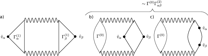
Figure 5: a) The Aslamazov-Larkin-type diagram corresponding to the term $\Gamma^{(1)}_{\alpha}\Gamma^{(1)}_{\beta}$. The product $\Gamma^{(0)}\Gamma^{(2)}_{\alpha\beta}$ comprises the Maki-Thompson-type diagram b) as well as self-energy correction c).

The resulting values (23) are most conveniently calculated in the local co-moving frame, where the hydrodynamic velocity entering the local equilibrium distribution functions in Eqs. (53) vanishes. The obtained results are then valid in arbitrary reference frame based on the principle that the relaxation are independent of the reference frame (generalizing the Galilean invariance to the arbitrary spectrum).

A.2 Dissipative corrections to the stress tensor

The collision integral ${\mathcal{C}}_{\pi}$ can be calculated along the same lines as ${\mathcal{C}}_{J}$ in the previous Section. Averaging the QKE with respect to the tensor quantities such as $v_{\alpha}v_{\beta}$, we find the contribution of the collision integral in the form similar to Eq. (49)

$${\mathcal{C}}_{\pi}\begin{pmatrix}\delta\Pi_{\alpha\beta}\cr\delta\Pi_{I,\alpha\beta}\cr T^{-1}\delta\Pi_{E,\alpha\beta}\end{pmatrix}=\left(\begin{array}[]{c}({v}_{\alpha}{v}_{\beta},\mathcal{C}\delta f^{(2)})\\ (\lambda{v}_{\alpha}{v}_{\beta},\mathcal{C}\delta f^{(2)})\\ (\varepsilon{v}_{\alpha}{v}_{\beta}/T,\mathcal{C}\delta f^{(2)})\end{array}\right).$$ (54)

The stress tensors were defined in Eqs. (26) and (27).

Defining the deviations from equilibrium as

$$\delta\Pi^{(k)}_{\alpha\beta}=\big{(}\phi_{k}{v}_{\alpha}{v}_{\beta},-\delta f^{(2)}\partial_{\varepsilon}f^{(0)}\big{)},$$ (55)

we can express the coefficients $g_{\alpha\beta}^{(j)}$ in the non-equilibrium distribution function (5) in terms of $\delta\Pi^{(k)}_{\alpha\beta}$. Similarly to the arguments presented in the previous Section, this yields the explicit form of the matrix collision integral ${\mathcal{C}}_{\pi}$:

$$[{C}_{\pi}]_{lk}=2\sum_{j=1}^{3}[\mathcal{M}^{-1}]_{jk}(\phi_{l}I_{\alpha\beta},\mathcal{C}\phi_{j}I_{\alpha\beta}).$$ (56)

Here the matrix $\mathcal{M}$ is given by Eq. (20b) and the traceless tensor $I_{\alpha\beta}$ is defined in Eq. (31c).

The matrix elements $(\phi_{l}I_{\alpha\beta},\mathcal{C}\phi_{j}I_{\alpha\beta})$ can be evaluated similarly to Eqs. (53):

$$(\phi I_{\alpha\beta},\mathcal{C}\phi^{\prime}I_{\gamma\delta})=\frac{1}{16\pi}\int\!d\omega\int\!d^{2}q\>\frac{|V(\omega,q)|^{2}}{\sinh^{2}(\omega/2T)}\bigg{[}\Xi^{(2)}_{\phi\phi^{\prime},\alpha\beta\gamma\delta}(\omega,q)\Gamma^{(0)}(\omega,q)-\Xi^{(1)}_{\phi,\alpha\beta}(\omega,q)\Xi^{(1)}_{\phi^{\prime},\gamma\delta}(\omega,q)\bigg{]}.$$ (57)

Here the tensor vertex functions are [$\lambda^{\prime}=\text{sign}(\varepsilon_{\lambda,\boldsymbol{p}}-\omega)$],

$$\Xi_{\phi,\alpha\beta}^{(1)}(\omega,q)=\frac{1}{T}\int_{\lambda,\boldsymbol{p}}\!\delta(\varepsilon_{\lambda,p}-\varepsilon_{\lambda^{\prime},\boldsymbol{p}+\boldsymbol{q}}+\omega)\left(f^{(0)}_{\lambda,p}-f^{(0)}_{\lambda^{\prime},\boldsymbol{p}+\boldsymbol{q}}\right)\Theta_{\lambda,\boldsymbol{p};\lambda^{\prime},\boldsymbol{p}+\boldsymbol{q}}\big{[}\phi_{\lambda^{\prime},\boldsymbol{p}+\boldsymbol{q}}\>I_{\alpha\beta,\boldsymbol{p}+\boldsymbol{q}}-\phi_{\lambda\boldsymbol{p}}\>I_{\alpha\beta,\boldsymbol{p}}\big{]},$$ (58a)

$$\Xi_{\phi\phi^{\prime},\alpha\beta\gamma\delta}^{(2)}(\omega,q)=\frac{1}{T}\int_{\lambda,\boldsymbol{p}}\!\delta(\varepsilon_{\lambda,p}-\varepsilon_{\lambda^{\prime},\boldsymbol{p}+\boldsymbol{q}}+\omega)\left(f^{(0)}_{\lambda,p}-f^{(0)}_{\lambda^{\prime},\boldsymbol{p}+\boldsymbol{q}}\right)\Theta_{\lambda,\boldsymbol{p};\lambda^{\prime},\boldsymbol{p}+\boldsymbol{q}}$$ (58b)

$$\qquad\qquad\qquad\qquad\times\big{[}\phi_{\lambda^{\prime},\boldsymbol{p}+\boldsymbol{q}}\>I_{\alpha\beta,\boldsymbol{p}+\boldsymbol{q}}-\phi_{\lambda\boldsymbol{p}}\>I_{\alpha\beta,\boldsymbol{p}}\big{]}\big{[}\phi^{\prime}_{\lambda^{\prime},\boldsymbol{p}+\boldsymbol{q}}\>I_{\gamma\delta,\boldsymbol{p}+\boldsymbol{q}}-\phi^{\prime}_{\lambda\boldsymbol{p}}\>I_{\gamma\delta,\boldsymbol{p}}\big{]}.$$

For further calculations it is useful to express the tensor $I_{\alpha\beta}$ in terms of the basis vectors $\{\hat{q}=\boldsymbol{q}/q,\hat{q}_{\perp}=\hat{z}\times\hat{q}\}$,

$$I_{\alpha\beta}=A_{\boldsymbol{k},\boldsymbol{q}}(2\hat{q}_{\alpha}\hat{q}_{\beta}-\delta_{\alpha\beta})+B_{\boldsymbol{k},\boldsymbol{q}}(\hat{q}_{\perp,\alpha}\hat{q}_{\beta}+\hat{q}_{\alpha}\hat{q}_{\perp,\beta})\>,$$ (59)

where

$$A_{\boldsymbol{k},\boldsymbol{q}}=\left(\frac{(\boldsymbol{k}\cdot\boldsymbol{q})^{2}}{(kq)^{2}}-1\right)+\frac{1}{2}=\tilde{A}_{\boldsymbol{k},\boldsymbol{q}}+\frac{1}{2},\qquad B_{\boldsymbol{k},\boldsymbol{q}}=\frac{(\boldsymbol{k}\cdot\boldsymbol{q}_{\perp})(\boldsymbol{k}\cdot\boldsymbol{q})}{k^{2}q^{2}}.$$ (60)

Due to the conservation laws of the electron-electron interaction we effectively have $A\rightarrow\tilde{A}$. Using the $\delta$-function in Eqs. (58a) and (58b) one obtains ($\varepsilon=\varepsilon_{\lambda,k}$),

$$\tilde{A}_{\boldsymbol{k},\boldsymbol{q}}=(\omega^{2}-q^{2})\>\frac{(2\varepsilon+\omega)^{2}-q^{2}}{8\varepsilon^{2}q^{2}}\>.$$ (61)

Furthermore, the coefficient $B$ drops out in the vertex function $\Xi^{(1)}$ since it is antisymmetric in the angle between $\boldsymbol{q}$ and $\boldsymbol{k}$. In the tensor vertex function $\Xi^{(2)}_{\alpha\beta\gamma\delta}(\omega,q)$ we get a separate contribution from $A$ and $B$ but they are orthogonal. For $B$ we obtain with the help of the $\delta$-functions ($\varepsilon=\varepsilon_{\lambda,k}$),

$$B_{\boldsymbol{k},\boldsymbol{q}}=\text{sign}(\boldsymbol{k}\cdot\hat{q}_{\perp})\frac{\sqrt{\left(q^{2}-\omega^{2}\right)[(2\varepsilon+\omega)^{2}-q^{2}]}\>(\omega^{2}-q^{2}-2\varepsilon\omega)}{4\varepsilon^{2}q^{2}}.$$ (62)

Finally, with the help of the angular averages

$$\int\!d\varphi_{q}\>\hat{q}_{\alpha}\hat{q}_{\beta}\hat{q}_{\gamma}\hat{q}_{\delta}=\frac{\pi}{4}(\delta_{\alpha\gamma}\delta_{\beta\delta}+\delta_{\alpha\delta}\delta_{\beta\gamma}+\delta_{\alpha\beta}\delta_{\gamma\delta}),$$

$$\int\!d\varphi_{q}\>(2\hat{q}_{\alpha}\hat{q}_{\beta}-\delta_{\alpha\beta})(2\hat{q}_{\gamma}\hat{q}_{\delta}-\delta_{\gamma\delta})=\pi(\delta_{\alpha\gamma}\delta_{\beta\delta}+\delta_{\alpha\delta}\delta_{\beta\gamma}-\delta_{\alpha\beta}\delta_{\gamma\delta}),$$

$$\int\!d\varphi_{q}\>(\hat{q}_{\perp,\alpha}\hat{q}_{\beta}+\hat{q}_{\alpha}\hat{q}_{\perp,\beta})(\hat{q}_{\perp,\gamma}\hat{q}_{\delta}+\hat{q}_{\gamma}\hat{q}_{\perp,\delta})=\pi(\delta_{\alpha\gamma}\delta_{\beta\delta}+\delta_{\alpha\delta}\delta_{\beta\gamma}-\delta_{\alpha\beta}\delta_{\gamma\delta})$$

and the projected quantities $\Xi^{(1,2)}$ obtained after averaging Eqs. (58) over the angle $\varphi_{q}$ of the transfered momentum $\boldsymbol{q}$,

$$\Xi_{\phi}^{(1)}(\omega,q)=\frac{1}{T}\int_{\lambda,\boldsymbol{p}}\!\delta(\varepsilon_{\lambda,p}-\varepsilon_{\lambda^{\prime},\boldsymbol{p}+\boldsymbol{q}}+\omega)\left(f^{(0)}_{\lambda,p}-f^{(0)}_{\lambda^{\prime},\boldsymbol{p}+\boldsymbol{q}}\right)\>\Theta_{\lambda,\boldsymbol{p};\lambda^{\prime},\boldsymbol{p}+\boldsymbol{q}}\big{[}\phi_{\lambda^{\prime},\boldsymbol{p}+\boldsymbol{q}}\>\tilde{A}_{\boldsymbol{k}+\boldsymbol{q},\boldsymbol{q}}-\phi_{\lambda\boldsymbol{p}}\tilde{A}_{\boldsymbol{k},\boldsymbol{q}}\big{]},$$ (63a)

$$\Xi_{\parallel,\phi\phi^{\prime}}^{(2)}(\omega,q)=\frac{1}{T}\int_{\lambda,\boldsymbol{p}}\!\delta(\varepsilon_{\lambda,p}-\varepsilon_{\lambda^{\prime},\boldsymbol{p}+\boldsymbol{q}}+\omega)\left(f^{(0)}_{\lambda,p}-f^{(0)}_{\lambda^{\prime},\boldsymbol{p}+\boldsymbol{q}}\right)\Theta_{\lambda,\boldsymbol{p};\lambda^{\prime},\boldsymbol{p}+\boldsymbol{q}}$$ (63b)

$$\qquad\qquad\quad\quad\quad\quad\times\big{[}\phi_{\lambda^{\prime},\boldsymbol{p}+\boldsymbol{q}}\>\tilde{A}_{\boldsymbol{p}+\boldsymbol{q},\boldsymbol{q}}-\phi_{\lambda\boldsymbol{p}}\>\tilde{A}_{\boldsymbol{p},\boldsymbol{q}}\big{]}\big{[}\phi^{\prime}_{\lambda^{\prime},\boldsymbol{p}+\boldsymbol{q}}\>\tilde{A}_{\boldsymbol{p}+\boldsymbol{q},\boldsymbol{q}}-\phi^{\prime}_{\lambda\boldsymbol{p}}\>\tilde{A}_{\boldsymbol{p},\boldsymbol{q}}\big{]},$$

$$\Xi_{\perp,\phi\phi^{\prime}}^{(2)}(\omega,q)=\frac{1}{T}\int_{\lambda,\boldsymbol{p}}\!\delta(\varepsilon_{\lambda,p}-\varepsilon_{\lambda^{\prime},\boldsymbol{p}+\boldsymbol{q}}+\omega)\left(f^{(0)}_{\lambda,p}-f^{(0)}_{\lambda^{\prime},\boldsymbol{p}+\boldsymbol{q}}\right)\Theta_{\lambda,\boldsymbol{p};\lambda^{\prime},\boldsymbol{p}+\boldsymbol{q}}$$ (63c)

$$\qquad\qquad\quad\quad\quad\quad\times\big{[}\phi_{\lambda^{\prime},\boldsymbol{p}+\boldsymbol{q}}\>B_{\boldsymbol{p}+\boldsymbol{q},\boldsymbol{q}}-\phi_{\lambda\boldsymbol{p}}\>B_{\boldsymbol{p},\boldsymbol{q}}\big{]}\big{[}\phi^{\prime}_{\lambda^{\prime},\boldsymbol{p}+\boldsymbol{q}}\>B_{\boldsymbol{p}+\boldsymbol{q},\boldsymbol{q}}-\phi^{\prime}_{\lambda\boldsymbol{p}}\>B_{\boldsymbol{p},\boldsymbol{q}}\big{]},$$

we can write the matrix elements as

$$(\phi I_{\alpha\beta},\mathcal{C}\phi^{\prime}I_{\gamma\delta})=\frac{1}{16\pi}(\delta_{\alpha\gamma}\delta_{\beta\delta}+\delta_{\alpha\delta}\delta_{\beta\gamma}-\delta_{\alpha\beta}\delta_{\gamma\delta})\int\!d\omega\int\!d^{2}q\frac{|V(\omega,q)|^{2}}{\sinh^{2}(\omega/2T)}$$ (64)

$$\qquad\qquad\bigg{[}\Xi^{(2)}_{\parallel,\phi\phi^{\prime}}(\omega,q)\Gamma^{(0)}(\omega,q)+\Xi^{(2)}_{\perp,\phi\phi^{\prime}}(\omega,q)\Gamma^{(0)}(\omega,q)-\Xi^{(1)}_{\phi}(\omega,q)\Xi^{(1)}_{\phi^{\prime}}(\omega,q)\bigg{]}.$$

Here we can drop the terms proportional to $\delta_{\alpha\beta}$ since the energy stress tensors are traceless. Due to their symmetry in $\alpha\leftrightarrow\beta$ we effectively have

$$\delta_{\alpha\gamma}\delta_{\beta\delta}+\delta_{\alpha\delta}\delta_{\beta\gamma}-\delta_{\alpha\beta}\delta_{\gamma\delta}\rightarrow 2\delta_{\alpha\gamma}\delta_{\beta\delta}.$$ (65)

The matrix elements (64) determine the quantities ${\cal C}_{\pi,ij}$, Eqs. (31), which in turn determine the viscosity (35).

Appendix B Linear response functions

In linear response we linearize the hydrodynamic equations with respect to the linear fluctuations of the hydrodynamic quantities, $\delta n$, $\delta n_{I}$, $\delta n_{E}$, $\delta u$:

$$n\rightarrow n+\delta n,\qquad n_{I}\rightarrow n_{I}+\delta n_{I},\qquad n_{E}\rightarrow n_{E}+\delta n_{E},\qquad u\rightarrow\delta u.$$ (66)

We furthermore introduce the response functions to the external perturbation $\boldsymbol{E}=-i\boldsymbol{q}\varphi$

$$\delta n=\chi_{n}\varphi,\qquad\delta n_{I}=\chi_{I}\varphi,\qquad\delta n_{E}=T\chi_{E}\varphi,\qquad\delta u=-i\frac{\boldsymbol{q}T}{qn_{E}}\chi_{u}\varphi.$$ (67)

Linearizing the continuity equations (39) and the Navier-Stokes equation (40), we find the matrix equation for the response functions $\chi_{i}$:

$$\begin{pmatrix}-i\omega+\frac{\tau_{1}}{2}q^{2}-2\pi eq\sigma_{0}&\frac{\tau_{2}}{2}q^{2}&-\left(\frac{n\tau_{1}+n_{I}\tau_{2}}{3n_{E}}T\right)q^{2}&\frac{nT}{n_{E}}q\cr\frac{\tau_{3}}{2}q^{2}-2\pi eq\sigma_{0}^{*}&-i\omega+\frac{\tau_{4}}{2}q^{2}&-\left(\frac{n_{I}\tau_{4}+n\tau_{3}}{3n_{E}}T\right)q^{2}&\frac{n_{I}T}{n_{E}}q\cr 0&0&-i\omega&\frac{3}{2}q\cr-\frac{4\pi e^{3}n}{3T}q&0&-\frac{q}{3}&-i\omega+\tau_{\rm dis}^{-1}+\frac{2\eta}{3n_{E}}q^{2}\end{pmatrix}\left(\begin{array}[]{c}\chi_{n}\\ \chi_{I}\\ \chi_{E}\\ \chi_{u}\end{array}\right)=\left(\begin{array}[]{c}-q^{2}\sigma_{0}/e\\ -q^{2}\sigma_{0}^{*}/e\\ 0\\ \frac{2en}{3T}q\end{array}\right),$$ (68)

where [cf. Eq. (42a)]

$$\sigma_{0}=e^{2}\!\left[\tau_{1}\left(\frac{\partial_{\mu}n}{2}-\frac{2n^{2}}{3n_{E}}\right)\!+\!\tau_{2}\left(\frac{\partial_{\mu}n_{I}}{2}-\frac{2nn_{I}}{3n_{E}}\right)\right],\qquad\sigma_{0}^{*}=e^{2}\!\left[\tau_{3}\left(\frac{\partial_{\mu}n}{2}-\frac{2n^{2}}{3n_{E}}\right)\!+\!\tau_{4}\left(\frac{\partial_{\mu}n_{I}}{2}-\frac{2nn_{I}}{3n_{E}}\right)\right].$$

The dispersion (II.2) of the collective modes follows from zeros of the determinant of the matrix in the left-hand side of Eq. (68).

In contrast to the energy waves and plasmons, which describe the response of the system to an external perturbation, the conductivity of an infinite system is defined as the response to the total electric field. Consequently, in order to find the conductivity (II.1), we need to consider the irreducible response functions, which satisfy the equation similar to Eq. (68), but without the Vlasov terms in the left column of the matrix in the left hand side. Then the conductivity is found from the Ohm’s law

$$\delta\boldsymbol{j}=(-i\boldsymbol{q}\varphi)\left[\sigma_{0}/e+\frac{1}{2}(\tau_{1}\chi_{n}+\tau_{2}\chi_{I})-\frac{n\tau_{1}+n_{I}\tau_{2}}{3n_{E}}T\chi_{E}+\frac{nT}{qn_{E}}\chi_{n}\right],$$ (69)

where $\varphi$ is now the total potential in the system (including the self-consistent Vlasov contribution).

References

- Landau and Lifshitz (2000) L. D. Landau and E. M. Lifshitz, Fluid mechanics (Butterworth-Heinemann, 2000).
- Lifshitz and Pitaevskii (1981) E. M. Lifshitz and L. P. Pitaevskii, Physical Kinetics (Butterworth-Heinemann, 1981).
- Vollhardt and Wölfle (1990) D. Vollhardt and P. Wölfle, The superfluid phases of Helium 3 (Taylor and Francis, 1990).
- Novoselov et al. (2004) K. S. Novoselov, A. K. Geim, S. V. Morozov, D. Jiang, Y. Zhang, S. V. Dubonos, I. V. Grigorieva, and A. A. Firsov, Science 306, 666 (2004).
- Hartnoll et al. (2007) S. A. Hartnoll, P. K. Kovtun, M. Müller, and S. Sachdev, Phys. Rev. B 76, 144502 (2007).
- Fritz et al. (2008) L. Fritz, J. Schmalian, M. Müller, and S. Sachdev, Phys. Rev. B 78, 085416 (2008).
- Müller et al. (2008) M. Müller, L. Fritz, and S. Sachdev, Phys. Rev. B 78, 115406 (2008).
- Müller and Sachdev (2008) M. Müller and S. Sachdev, Phys. Rev. B 78, 115419 (2008).
- Müller et al. (2009) M. Müller, L. Fritz, S. Sachdev, and J. Schmalian, AIP Conference Proceedings 1134, 170 (2009).
- Foster and Aleiner (2009) M. S. Foster and I. L. Aleiner, Phys. Rev. B 79, 085415 (2009).
- Müller et al. (2009) M. Müller, J. Schmalian, and L. Fritz, Phys. Rev. Lett. 103, 025301 (2009).
- Svintsov et al. (2012) D. Svintsov, V. Vyurkov, S. Yurchenko, T. Otsuji, and V. Ryzhii, Journal of Applied Physics 111, 083715 (2012).
- Tomadin and Polini (2013) A. Tomadin and M. Polini, Phys. Rev. B 88, 205426 (2013).
- Svintsov et al. (2013) D. Svintsov, V. Vyurkov, V. Ryzhii, and T. Otsuji, Phys. Rev. B 88, 245444 (2013).
- Phan et al. (2013) T. V. Phan, J. C. W. Song, and L. S. Levitov (2013), arXiv:1306.4972 (unpublished).
- Levitov et al. (2013) L. S. Levitov, A. V. Shtyk, and M. V. Feigelman, Phys. Rev. B 88, 235403 (2013).
- Tomadin et al. (2014) A. Tomadin, G. Vignale, and M. Polini, Phys. Rev. Lett. 113, 235901 (2014).
- Narozhny et al. (2015) B. N. Narozhny, I. V. Gornyi, M. Titov, M. Schütt, and A. D. Mirlin, Phys. Rev. B 91, 035414 (2015).
- Principi et al. (2015) A. Principi, G. Vignale, M. Carrega, and M. Polini (2015), arXiv:1506.06030 (unpublished).
- Maier (2012) S. A. Maier, Nature Phys. 8, 581 (2012).
- Grigorenko et al. (2012) A. N. Grigorenko, M. Polini, and K. S. Novoselov, Nat Photon 6, 749 (2012).
- Damle and Sachdev (1997) K. Damle and S. Sachdev, Phys. Rev. B 56, 8714 (1997).
- Principi et al. (2013) A. Principi, G. Vignale, M. Carrega, and M. Polini, Phys. Rev. B 88, 195405 (2013).
- Schütt et al. (2013) M. Schütt, P. M. Ostrovsky, M. Titov, I. V. Gornyi, B. N. Narozhny, and A. D. Mirlin, Phys. Rev. Lett. 110, 026601 (2013).
- Song and Levitov (2013) J. C. W. Song and L. S. Levitov, Phys. Rev. Lett. 111, 126601 (2013).
- Titov et al. (2013) M. Titov, R. V. Gorbachev, B. N. Narozhny, T. Tudorovskiy, M. Schütt, P. M. Ostrovsky, I. V. Gornyi, A. D. Mirlin, M. I. Katsnelson, K. S. Novoselov, et al., Phys. Rev. Lett. 111, 166601 (2013).
- Basov et al. (2014) D. N. Basov, M. M. Fogler, A. Lanzara, F. Wang, and Y. Zhang, Rev. Mod. Phys. 86, 959 (2014).
- Fei et al. (2012) Z. Fei, A. S. Rodin, G. O. Andreev, W. Bao, A. S. McLeod, M. Wagner, L. M. Zhang, Z. Zhao, M. Thiemens, G. Dominguez, et al., Nature 487, 82 (2012).
- Chen et al. (2012) J. Chen, M. Badioli, P. Alonso-Gonzalez, S. Thongrattanasiri, F. Huth, J. Osmond, M. Spasenovic, A. Centeno, A. Pesquera, P. Godignon, et al., Nature 487, 77 (2012).
- Abanin et al. (2011) D. A. Abanin, S. V. Morozov, L. A. Ponomarenko, R. V. Gorbachev, A. S. Mayorov, M. I. Katsnelson, K. Watanabe, T. Taniguchi, K. S. Novoselov, L. S. Levitov, et al., Science 332, 328 (2011).
- Taychatanapat et al. (2013) T. Taychatanapat, K. Watanabe, T. Taniguchi, and P. Jarillo-Herrero, Nature Phys. 9, 225 (2013).
- Alonso-González et al. (2014) P. Alonso-González, A. Y. Nikitin, F. Golmar, A. Centeno, A. Pesquera, S. Vélez, J. Chen, G. Navickaite, F. Koppens, A. Zurutuza, et al., Science 344, 1369 (2014).
- Woessner et al. (2015) A. Woessner, M. B. Lundeberg, Y. Gao, A. Principi, P. Alonso-Gonzalez, M. Carrega, K. Watanabe, T. Taniguchi, G. Vignale, M. Polini, et al., Nature Materials 14, 421 (2015).
- Ponomarenko et al. (2011) L. A. Ponomarenko, A. K. Geim, A. A. Zhukov, R. Jalil, S. V. Morozov, K. S. Novoselov, I. V. Grigorieva, E. H. Hill, V. V. Cheianov, V. I. Fal’ko, et al., Nature Phys. 7, 958 (2011).
- Decker et al. (2011) R. Decker, Y. Wang, V. W. Brar, W. Regan, H.-Z. Tsai, Q. Wu, W. Gannett, A. Zettl, and M. F. Crommie, Nano Letters 11, 2291 (2011).
- Kashuba (2008) A. B. Kashuba, Phys. Rev. B 78, 085415 (2008).
- Schütt et al. (2011) M. Schütt, P. M. Ostrovsky, I. V. Gornyi, and A. D. Mirlin, Phys. Rev. B 83, 155441 (2011).
- Tomadin et al. (2013) A. Tomadin, D. Brida, G. Cerullo, A. C. Ferrari, and M. Polini, Phys. Rev. B 88, 035430 (2013).
- Kozikov et al. (2010) A. A. Kozikov, A. K. Savchenko, B. N. Narozhny, and A. V. Shytov, Phys. Rev. B 82, 075424 (2010).
- Sheehy and Schmalian (2007) D. E. Sheehy and J. Schmalian, Phys. Rev. Lett. 99, 226803 (2007).
- Chapman (1916) S. Chapman, Phil. Trans. R. Soc. Lond. A 216, 279 (1916).
- Chapman (1918) S. Chapman, Phil. Trans. R. Soc. Lond. A 217, 115 (1918).
- Enskog (1921) D. Enskog, Arkiv Mat. Astr. Fys. 16, 60 (1921).
- Arnold et al. (2000) P. Arnold, G. D. Moore, and L. G. Yaffe, Journal of High Energy Physics 2000, 001 (2000).
- Sunyaev and Zeldovich (1970) R. Sunyaev and Y. B. Zeldovich, Astrophysics and Space Science 7 (1970).
- Peebles and Yu (1970) P. J. E. Peebles and J. T. Yu, The Astrophysical Journal 162 (1970).
- Zala et al. (2001) G. Zala, B. N. Narozhny, and I. L. Aleiner, Phys. Rev. B 64, 214204 (2001).
- Hwang and Das Sarma (2007) E. H. Hwang and S. Das Sarma, Phys. Rev. B 75, 205418 (2007).
- Stauber (2014) T. Stauber, J. Phys.: Condens. Matter 26, 123201 (2014).
- Ascher et al. (1995) U. M. Ascher, S. J. Ruuth, and B. T. R. Wetton, SIAM Journal on Numerical Analysis 32, 797 (1995).
- Griebel et al. (1997) M. Griebel, T. Dornsheifer, and T. Neunhoeffer, Numerical Simulation in Fluid Dynamics (Society for Industrial and Applied Mathematics, 1997).