Formalism for the solution of quadratic Hamiltonians with large cosine terms

Abstract

We consider quantum Hamiltonians of the form $H=H_{0}-U\sum_{j}\cos(C_{j})$ where $H_{0}$ is a quadratic function of position and momentum variables $\{x_{1},p_{1},x_{2},p_{2},...\}$ and the $C_{j}$’s are linear in these variables. We allow $H_{0}$ and $C_{j}$ to be completely general with only two restrictions: we require that (1) the $C_{j}$’s are linearly independent and (2) $[C_{j},C_{k}]$ is an integer multiple of $2\pi i$ for all $j,k$ so that the different cosine terms commute with one another. Our main result is a recipe for solving these Hamiltonians and obtaining their exact low energy spectrum in the limit $U\rightarrow\infty$. This recipe involves constructing creation and annihilation operators and is similar in spirit to the procedure for diagonalizing quadratic Hamiltonians. In addition to our exact solution in the infinite $U$ limit, we also discuss how to analyze these systems when $U$ is large but finite. Our results are relevant to a number of different physical systems, but one of the most natural applications is to understanding the effects of electron scattering on quantum Hall edge modes. To demonstrate this application, we use our formalism to solve a toy model for a fractional quantum spin Hall edge with different types of impurities.

I Introduction

In this paper we study a general class of quantum Hamiltonians which are relevant to a number of different physical systems. The Hamiltonians we consider are defined on a $2N$ dimensional phase space $\{x_{1},...,x_{N},p_{1},...,p_{N}\}$ with $[x_{i},p_{j}]=i\delta_{ij}$. They take the form

$$H=H_{0}-U\sum_{i=1}^{M}\cos(C_{i})$$ (1)

where $H_{0}$ is a quadratic function of the phase space variables $\{x_{1},...,x_{N},p_{1},...,p_{N}\}$, and $C_{i}$ is linear in these variables. The $C_{i}$’s can be chosen arbitrarily except for two restrictions:

1. $\{C_{1},...,C_{M}\}$ are linearly independent.

2. $[C_{i},C_{j}]$ is an integer multiple of $2\pi i$ for all $i,j$.

Here, the significance of the second condition is that it guarantees that the cosine terms commute with one another: $[\cos(C_{i}),\cos(C_{j})]=0$ for all $i,j$.

For small $U$, we can straightforwardly analyze these Hamiltonians by treating the cosine terms as perturbations to $H_{0}$. But how can we study these systems when $U$ is large? The most obvious approach is to expand around $U=\infty$, just as in the small $U$ case we expand around $U=0$. But in order to make such an expansion, we first need to be able to solve these Hamiltonians exactly in the infinite $U$ limit. The purpose of this paper is to describe a systematic procedure for obtaining such a solution, at least at low energies.

The basic idea underlying our solution is that when $U$ is very large, the cosine terms act as constraints at low energies. Thus, the low energy spectrum of $H$ can be described by an effective Hamiltonian $H_{\text{eff}}$ defined within a constrained Hilbert space $\mathcal{H}_{\text{eff}}$. This effective Hamiltonian $H_{\text{eff}}$ is quadratic in $\{x_{1},...,x_{N},p_{1},...,p_{N}\}$ since $H_{0}$ is quadratic and the constraints are linear in these variables. We can therefore diagonalize $H_{\text{eff}}$ and in this way determine the low energy properties of $H$.

Our main result is a general recipe for finding the exact low energy spectrum of $H$ in the limit $U\rightarrow\infty$. This recipe consists of two steps and is only slightly more complicated than what is required to solve a conventional quadratic Hamiltonian. The first step involves finding creation and annihilation operators for the low energy effective Hamiltonian $H_{\text{eff}}$ (Eq. 11). The second step of the recipe involves finding integer linear combinations of the $C_{i}$’s that have simple commutation relations with one another. In practice, this step amounts to finding a change of basis that puts a particular integer skew-symmetric matrix into canonical form (Eq. 14). Once these two steps are completed, the low energy spectrum can be written down immediately (Eq. 19).

In addition to our exact solution in the infinite $U$ limit, we also discuss how to analyze these systems when $U$ is large but finite. In particular, we show that in the finite $U$ case, we need to add small (non-quadratic) corrections to the effective Hamiltonian $H_{\text{eff}}$ in order to reproduce the low energy physics of $H$. One of our key results is a discussion of the general form of these finite $U$ corrections, and how they scale with $U$.

Our results are useful because there are a number of physical systems where one needs to understand the effect of cosine-like interactions on a quadratic Hamiltonian. An important class of examples are the edges of Abelian fractional quantum Hall (FQH) states. Previously it has been argued that a general Abelian FQH edge can be modeled as collection of $p$ chiral Luttinger liquids with Hamiltonian Wen (1990); Frohlich and Kerler (1991); Wen (1995, 2007)

$$H_{0}=\int dx\frac{1}{4\pi}(\partial_{x}\Phi)^{T}V(\partial_{x}\Phi)$$

Here $\Phi(x)=(\phi_{1}(x),...,\phi_{p}(x))$, with each component $\phi_{I}$ describing a different (bosonized) edge mode while $V$ is a $p\times p$ matrix that describes the velocities and density-density interactions between the different edge modes. The commutation relations for the $\phi_{I}$ operators are $[\phi_{I}(x),\partial_{y}\phi_{J}(y)]=2\pi i(K^{-1})_{IJ}\delta(x-y)$ where $K$ is a symmetric, integer $p\times p$ matrix which is determined by the bulk FQH state.

The above Hamiltonian $H_{0}$ is quadratic and hence exactly soluble, but in many cases it is unrealistic because it describes an edge in which electrons do not scatter between the different edge modes. In order to incorporate scattering into the model, we need to add terms to the Hamiltonian of the form

$$H_{\text{scat}}=\int U(x)\cos(\Lambda^{T}K\Phi-\alpha(x))dx$$

where $\Lambda$ is a $p$-component integer vector that describes the number of electrons scattered from each edge mode Kane and Fisher (1995). However, it is usually difficult to analyze the effect of these cosine terms beyond the small $U$ limit where perturbative techniques are applicable. (An important exception is when $\Lambda$ is a null vector Haldane (1995), i.e. $\Lambda^{T}K\Lambda=0$: in this case, the fate of the edge modes can be determined by mapping the system onto a Sine-Gordon model Wang and Levin (2013)).

Our results can provide insight into this class of systems because they allow us to construct exactly soluble toy models that capture the effect of electron scattering at the edge. Such toy models can be obtained by replacing the above continuum scattering term $H_{\text{scat}}$ by a collection of discrete impurity scatterers, $U\sum_{i}\cos(\Lambda^{T}K\Phi(x_{i})-\alpha_{i})$, and then taking the limit $U\rightarrow\infty$. It is not hard to see that the latter cosine terms obey conditions (1) and (2) from above, so we can solve the resulting models exactly using our general recipe. Importantly, this construction is valid for any choice of $\Lambda$, whether or not $\Lambda$ is a null vector.

Although the application to FQH edge states is one of the most interesting aspects of our results, our focus in this paper is on the general formalism rather than the implications for specific physical systems. Therefore, we will only present a few simple examples involving a fractional quantum spin Hall edge with different types of impurities. The primary purpose of these examples is to demonstrate how our formalism works rather than to obtain novel results.

We now discuss the relationship with previous work. One paper that explores some related ideas is Ref. Gottesman et al., 2001. In that paper, Gottesman, Kitaev, and Preskill discussed Hamiltonians similar to (1) for the case where the $C_{i}$ operators do not commute, i.e. $[C_{i},C_{j}]\neq 0$. They showed that these Hamiltonians can have degenerate ground states and proposed using these degenerate states to realize qubits in continuous variable quantum systems.

Another line of research that has connections to the present work involves the problem of understanding constraints in quantum mechanics. In particular, a number of previous works have studied the problem of a quantum particle that is constrained to move on a surface by a strong confining potential Jensen and Koppe (1971); Da Costa (1981). This problem is similar in spirit to one we study here, particularly for the special case where $[C_{i},C_{j}]=0$: in that case, if we identify $C_{i}$ as position coordinates $x_{i}$, then the Hamiltonian (1) can be thought of as describing a particle that is constrained to move on a periodic array of hyperplanes.

Our proposal to apply our formalism to FQH edge states also has connections to the previous literature. In particular, it has long been known that the problem of an impurity in a non-chiral Luttinger liquid has a simple exact solution in the limit of infinitely strong backscattering Kane and Fisher (1992a, b); d. C. Chamon et al. (1996); Chamon et al. (1995). The infinite backscattering limit for a single impurity has also been studied for more complicated Luttinger liquid systems Chklovskii and Halperin (1998); Chamon and Fradkin (1997); Ponomarenko and Averin (2007); Ganeshan et al. (2012). The advantage of our approach to these systems is that our methods allow us to study not just single impurities but also multiple coherently coupled impurities, and to obtain the full quantum dynamics not just transport properties.

The paper is organized as follows. In section II we summarize our formalism and main results. In section III we illustrate our formalism with some examples involving fractional quantum spin Hall edges with impurities. We discuss directions for future work in the conclusion. The appendices contain the general derivation of our formalism as well as other technical results.

II Summary of results

II.1 Low energy effective theory

Our first result is that we derive an effective theory that describes the low energy spectrum of

$$H=H_{0}-U\sum_{i=1}^{M}\cos(C_{i})$$

in the limit $U\rightarrow\infty$. This effective theory consists of an effective Hamiltonian $H_{\text{eff}}$ and an effective Hilbert space $\mathcal{H}_{\text{eff}}$. Conveniently, we find a simple algebraic expression for $H_{\text{eff}}$ and $\mathcal{H}_{\text{eff}}$ that holds in the most general case. Specifically, the effective Hamiltonian is given by

$$H_{\text{eff}}=H_{0}-\sum_{i,j=1}^{M}\frac{(\mathcal{M}^{-1})_{ij}}{2}\cdot\Pi_{i}\Pi_{j}$$ (2)

where the operators $\Pi_{1},...,\Pi_{M}$ are defined by

$$\Pi_{i}=\frac{1}{2\pi i}\sum_{j=1}^{M}\mathcal{M}_{ij}[C_{j},H_{0}]$$ (3)

and where $\mathcal{M}_{ij}$ is an $M\times M$ matrix defined by

$$\mathcal{M}=\mathcal{N}^{-1},\quad\mathcal{N}_{ij}=-\frac{1}{4\pi^{2}}[C_{i},[C_{j},H_{0}]]$$ (4)

This effective Hamiltonian is defined on an effective Hilbert space $\mathcal{H}_{\text{eff}}$, which is a subspace of the original Hilbert space $\mathcal{H}$, and consists of all states $|\psi\rangle$ that satisfy

$$\cos(C_{i})|\psi\rangle=|\psi\rangle,\quad i=1,...,M$$ (5)

A few remarks about these formulas: first, notice that $\mathcal{M}$ and $\mathcal{N}$ are matrices of $c$-numbers since $H_{0}$ is quadratic and the $C_{i}$’s are linear combinations of $x_{j}$’s and $p_{j}$’s. Also notice that the $\Pi_{i}$ operators are linear functions of $\{x_{1},...,x_{N},p_{1},...,p_{N}\}$. These observations imply that the effective Hamiltonian $H_{\text{eff}}$ is always quadratic. Another important point is that the $\Pi_{i}$ operators are conjugate to the $C_{i}$’s:

$$[C_{i},\Pi_{j}]=2\pi i\delta_{ij}$$ (6)

This means that we can think of the $\Pi_{i}$’s as generalized momentum operators. Finally, notice that

$$[C_{i},H_{\text{eff}}]=0$$ (7)

The significance of this last equation is that it shows that the Hamiltonian $H_{\text{eff}}$ can be naturally defined within the above Hilbert space (5).

We can motivate this effective theory as follows. First, it is natural to expect that the lowest energy states in the limit $U\rightarrow\infty$ are those that minimize the cosine terms. This leads to the effective Hilbert space given in Eq. 5. Second, it is natural to expect that the dynamics in the $C_{1},...,C_{M}$ directions freezes out at low energies. Hence, the terms that generate this dynamics, namely $\sum_{ij}\frac{\mathcal{M}^{-1}_{ij}}{2}\Pi_{i}\Pi_{j}$, should be removed from the effective Hamiltonian. This leads to Eq. 2. Of course this line of reasoning is just an intuitive picture; for a formal derivation of the effective theory, we refer the reader to appendix A.

At what energy scale is the above effective theory valid? We show that $H_{\text{eff}}$ correctly reproduces the energy spectrum of $H$ for energies less than $\sqrt{U/m}$ where $m$ is the maximum eigenvalue of $\mathcal{M}_{ij}$. One implication of this result is that our effective theory is only valid if $\mathcal{N}$ is non-degenerate: if $\mathcal{N}$ were degenerate than $\mathcal{M}$ would have an infinitely large eigenvalue, which would mean that there would be no energy scale below which our theory is valid. Physically, the reason that our effective theory breaks down when $\mathcal{N}$ is degenerate is that in this case, the dynamics in the $C_{1},...,C_{M}$ directions does not completely freeze out at low energies.

To see an example of these results, consider a one dimensional harmonic oscillator with a cosine term:

$$H=\frac{p^{2}}{2m}+\frac{Kx^{2}}{2}-U\cos(2\pi x)$$ (8)

In this case, we have $H_{0}=\frac{p^{2}}{2m}+\frac{Kx^{2}}{2}$ and $C=2\pi x$. If we substitute these expressions into Eq. 2, a little algebra gives

$$H_{\text{eff}}=\frac{Kx^{2}}{2}$$

As for the effective Hilbert space, Eq. 5 tells us that $\mathcal{H}_{\text{eff}}$ consists of position eigenstates

$$\mathcal{H}_{\text{eff}}=\{|x=q\rangle,\quad q=\text{(integer)}\}$$

If we now diagonalize the effective Hamiltonian within the effective Hilbert space, we obtain eigenstates $|x=q\rangle$ with energies $E=\frac{Kq^{2}}{2}$. Our basic claim is that these eigenstates and energies should match the low energy spectrum of $H$ in the $U\rightarrow\infty$ limit. In appendix A.1.1, we analyze this example in detail and we confirm that this claim is correct (up to a constant shift in the energy spectrum).

To see another illustrative example, consider a one dimensional harmonic oscillator with two cosine terms,

$$H=\frac{p^{2}}{2m}+\frac{Kx^{2}}{2}-U\cos(dp)-U\cos(2\pi x)$$ (9)

where $d$ is a positive integer. This example is fundamentally different from the previous one because the arguments of the cosine do not commute: $[x,p]\neq 0$. This property leads to some new features, such as degeneracies in the low energy spectrum. To find the effective theory in this case, we note that $H_{0}=\frac{p^{2}}{2m}+\frac{Kx^{2}}{2}$ and $C_{1}=dp$, $C_{2}=2\pi x$. With a little algebra, Eq. 2 gives

$$H_{\text{eff}}=0$$

As for the effective Hilbert space, Eq. 5 tells us that $\mathcal{H}_{\text{eff}}$ consists of all states $|\psi\rangle$ satisfying

$$\cos(2\pi x)|\psi\rangle=\cos(dp)|\psi\rangle=|\psi\rangle.$$

One can check that there are $d$ linearly independent states obeying the above conditions; hence if we diagonalize the effective Hamiltonian within the effective Hilbert space, we obtain $d$ exactly degenerate eigenstates with energy $E=0$. The prediction of our formalism is therefore that $H$ has a $d$-fold ground state degeneracy in the $U\rightarrow\infty$ limit. In appendix A.1.2, we analyze this example and confirm this prediction.

II.2 Diagonalizing the effective theory

We now move on to discuss our second result, which is a recipe for diagonalizing the effective Hamiltonian $H_{\text{eff}}$. Note that this diagonalization procedure is unnecessary for the two examples discussed above, since $H_{\text{eff}}$ is very simple in these cases. However, in general, $H_{\text{eff}}$ is a complicated quadratic Hamiltonian which is defined within a complicated Hilbert space $\mathcal{H}_{\text{eff}}$, so diagonalization is an important issue. In fact, in practice, the results in this section are more useful than those in the previous section because we will see that we can diagonalize $H_{\text{eff}}$ without explicitly evaluating the expression in Eq. 2.

Our recipe for diagonalizing $H_{\text{eff}}$ has three steps. The first step is to find creation and annihilation operators for $H_{\text{eff}}$. Formally, this amounts to finding all operators $a$ that are linear combinations of $\{x_{1},...,x_{N},p_{1},...,p_{N}\}$, and satisfy

$$[a,H_{\text{eff}}] =Ea,$$

$$[a,C_{i}] =0,\quad i=1,...,M$$ (10)

for some scalar $E\neq 0$. While the first condition is the usual definition of creation and annihilation operators, the second condition is less standard; the motivation for this condition is that $H_{\text{eff}}$ commutes with $C_{i}$ (see Eq. 7). As a result, we can impose the requirement $[a,C_{i}]=0$ and we will still have enough quantum numbers to diagonalize $H_{\text{eff}}$ since we can use the $C_{i}$’s in addition to the $a$’s.

Alternatively, there is another way to find creation and annihilation operators which is often more convenient: instead of looking for solutions to (10), one can look for solutions to

$$[a,H_{0}] =Ea+\sum_{j=1}^{M}\lambda_{j}[C_{j},H_{0}],$$

$$[a,C_{i}] =0,\quad i=1,...,M$$ (11)

for some scalars $E,\lambda_{j}$ with $E\neq 0$. Indeed, we show in appendix B.4 that every solution to (10) is also a solution to (11) and vice versa, so these two sets of equations are equivalent. In practice, it is easier to work with Eq. 11 than Eq. 10 because Eq. 11 is written in terms of $H_{0}$, and thus it does not require us to work out the expression for $H_{\text{eff}}$.

The solutions to (10), or equivalently (11), can be divided into two classes: “annihilation operators” with $E>0$, and “creation operators” with $E<0$. Let $a_{1},...,a_{K}$ denote a complete set of linearly independent annihilation operators. We will denote the corresponding $E$’s by $E_{1},...,E_{K}$ and the creation operators by $a_{1}^{\dagger},...,a_{K}^{\dagger}$. The creation/annihilation operators should be normalized so that

$$[a_{k},a_{k^{\prime}}^{\dagger}]=\delta_{kk^{\prime}},\quad[a_{k},a_{k^{\prime}}]=[a_{k}^{\dagger},a_{k^{\prime}}^{\dagger}]=0$$

We are now ready to discuss the second step of the recipe. This step involves searching for linear combinations of $\{C_{1},...,C_{M}\}$ that have simple commutation relations with one another. The idea behind this step is that we ultimately need to construct a complete set of quantum numbers for labeling the eigenstates of $H_{\text{eff}}$. Some of these quantum numbers will necessarily involve the $C_{i}$ operators since these operators play a prominent role in the definition of the effective Hilbert space, $\mathcal{H}_{\text{eff}}$. However, the $C_{i}$’s are unwieldy because they have complicated commutation relations with one another. Thus, it is natural to look for linear combinations of $C_{i}$’s that have simpler commutation relations.

With this motivation in mind, let $\mathcal{Z}_{ij}$ be the $M\times M$ matrix defined by

$$\mathcal{Z}_{ij}=\frac{1}{2\pi i}[C_{i},C_{j}]$$ (12)

The matrix $\mathcal{Z}_{ij}$ is integer and skew-symmetric, but otherwise arbitrary. Next, let

$$C_{i}^{\prime}=\sum_{j=1}^{M}\mathcal{V}_{ij}C_{j}{\color[rgb]{0,0,0}+\chi_{i}}$$ (13)

for some matrix $\mathcal{V}$ and some vector $\chi$. Then, $[C_{i}^{\prime},C_{j}^{\prime}]=2\pi i\mathcal{Z}_{ij}^{\prime}$ where $\mathcal{Z}^{\prime}=\mathcal{V}\mathcal{Z}\mathcal{V}^{T}$. The second step of the recipe is to find a matrix $\mathcal{V}$ with integer entries and determinant $\pm 1$, such that $\mathcal{Z}^{\prime}$ takes the simple form

$$\mathcal{Z}^{\prime}=\begin{pmatrix}0_{I}&-\mathcal{D}&0\\ \mathcal{D}&0_{I}&0\\ 0&0&0_{M-2I}\end{pmatrix},\quad\mathcal{D}=\begin{pmatrix}d_{1}&0&\dots&0\\ 0&d_{2}&\dots&0\\ \vdots&\vdots&\vdots&\vdots\\ 0&0&\dots&d_{I}\end{pmatrix}$$ (14)

Here $I$ is some integer with $0\leq I\leq M/2$ and $0_{I}$ denotes an $I\times I$ matrix of zeros. In mathematical language, $\mathcal{V}$ is an integer change of basis that puts $\mathcal{Z}$ into skew-normal form. It is known that such a change of basis always exists, though it is not unique.Newman (1972) After finding an appropriate $\mathcal{V}$, the offset $\chi$ should then be chosen so that

$$\chi_{i}=\pi\cdot\sum_{j<k}\mathcal{V}_{ij}\mathcal{V}_{ik}\mathcal{Z}_{jk}\pmod{2\pi}$$ (15)

The reason for choosing $\chi$ in this way is that it ensures that $e^{iC_{i}^{\prime}}|\psi\rangle=|\psi\rangle$ for any $|\psi\rangle\in\mathcal{H}_{\text{eff}}$, as can be easily seen from the Campbell-Baker-Hausdorff formula.

Once we perform these two steps, we can obtain the complete energy spectrum of $H_{\text{eff}}$ with the help of a few results that we prove in appendix B. Our first result is that $H_{\text{eff}}$ can always be written in the form

$$H_{\text{eff}}=\sum_{k=1}^{K}E_{k}a_{k}^{\dagger}a_{k}+F\left(C_{2I+1}^{\prime},...,C_{M}^{\prime}\right)$$ (16)

where $F$ is some (a priori unknown) quadratic function. Our second result (which is really just an observation) is that the following operators all commute with each other:

$$\{e^{iC_{1}^{\prime}/d_{1}},...,e^{iC_{I}^{\prime}/d_{I}},e^{iC_{I+1}^{\prime}},...,e^{iC_{2I}^{\prime}},C_{2I+1}^{\prime},...,C_{M}^{\prime}\}$$ (17)

Furthermore, these operators commute with the occupation number operators $\{a_{1}^{\dagger}a_{1},...,a_{K}^{\dagger}a_{K}\}$. Therefore, we can simultaneously diagonalize (17) along with $\{a_{k}^{\dagger}a_{k}\}$. We denote the simultaneous eigenstates by

$$|\theta_{1},...,\theta_{I},\varphi_{1},...,\varphi_{I},x_{I+1}^{\prime},...,x_{M-I}^{\prime},n_{1},...,n_{K}\rangle$$

or, in more abbreviated form, $|\boldsymbol{\theta},\boldsymbol{\varphi},\boldsymbol{x}^{\prime},\boldsymbol{n}\rangle$. Here the different quantum numbers are defined by

$$e^{iC_{i}^{\prime}/d_{i}}|\boldsymbol{\theta},\boldsymbol{\varphi},\boldsymbol{x}^{\prime},\boldsymbol{n}\rangle=e^{i\theta_{i}}|\boldsymbol{\theta},\boldsymbol{\varphi},\boldsymbol{x}^{\prime},\boldsymbol{n}\rangle,\ i=1,...,I$$

$$e^{iC_{i}^{\prime}}|\boldsymbol{\theta},\boldsymbol{\varphi},\boldsymbol{x}^{\prime},\boldsymbol{n}\rangle=e^{i\varphi_{i-I}}|\boldsymbol{\theta},\boldsymbol{\varphi},\boldsymbol{x}^{\prime},\boldsymbol{n}\rangle,\ i=I+1,...,2I$$

$$C_{i}^{\prime}|\boldsymbol{\theta},\boldsymbol{\varphi},\boldsymbol{x}^{\prime},\boldsymbol{n}\rangle=2\pi x_{i-I}^{\prime}|\boldsymbol{\theta},\boldsymbol{\varphi},\boldsymbol{x}^{\prime},\boldsymbol{n}\rangle,\ i=2I+1,...,M$$

$$a_{k}^{\dagger}a_{k}|\boldsymbol{\theta},\boldsymbol{\varphi},\boldsymbol{x}^{\prime},\boldsymbol{n}\rangle=n_{k}|\boldsymbol{\theta},\boldsymbol{\varphi},\boldsymbol{x}^{\prime},\boldsymbol{n}\rangle,\ k=1,...,K$$ (18)

where $0\leq\theta_{i},\varphi_{i}<2\pi$, while $x_{i}^{\prime}$ is real valued and $n_{k}$ ranges over non-negative integers.

By construction the $|\boldsymbol{\theta},\boldsymbol{\varphi},\boldsymbol{x}^{\prime},\boldsymbol{n}\rangle$ states form a complete basis for the Hilbert space $\mathcal{H}$. Our third result is that a subset of these states form a complete basis for the effective Hilbert space $\mathcal{H}_{\text{eff}}$. This subset consists of all $|\boldsymbol{\theta},\boldsymbol{\varphi},\boldsymbol{x}^{\prime},\boldsymbol{n}\rangle$ for which

1. $\boldsymbol{\theta}=(2\pi\alpha_{1}/d_{1},...,2\pi\alpha_{I}/d_{I})$ with $\alpha_{i}=0,1,...,d_{i}-1$.

2. $\boldsymbol{\varphi}=(0,0,...,0)$.

3. $(x_{I+1}^{\prime},...,x_{M-I}^{\prime})=(q_{1},...,q_{M-2I})$ for some integers $q_{i}$.

We will denote this subset of eigenstates by $\{|\boldsymbol{\alpha},\boldsymbol{q},\boldsymbol{n}\rangle\}$.

Putting this together, we can see from equations (16) and (18) that the $|\boldsymbol{\alpha},\boldsymbol{q},\boldsymbol{n}\rangle$ are eigenstates of $H_{\text{eff}}$, with eigenvalues

$$E=\sum_{k=1}^{K}n_{k}E_{k}+F(2\pi q_{1},...,2\pi q_{M-2I})$$ (19)

We therefore have the full eigenspectrum of $H_{\text{eff}}$ — up to the determination of the function $F$. With a bit more work, one can go further and compute the function $F$ (see appendix B.3) but we will not discuss this issue here because in many cases of interest it is more convenient to find $F$ using problem-specific approaches.

To see examples of this diagonalization procedure, we refer the reader to section III. As for the general derivation of this procedure, see appendix B.

II.3 Degeneracy

One implication of Eq. 19 which is worth mentioning is that the energy $E$ is independent of the quantum numbers $\alpha_{1},...,\alpha_{I}$. Since $\alpha_{i}$ ranges from $0\leq\alpha_{i}<d_{i}-1$, it follows that every eigenvalue of $H_{\text{eff}}$ has a degeneracy of (at least)

$$D=\prod_{i=1}^{I}d_{i}$$ (20)

In the special case where $\mathcal{Z}_{ij}$ is non-degenerate (i.e. the case where $M=2I$), this degeneracy can be conveniently written as

$$D=\sqrt{\det(\mathcal{Z})}$$ (21)

since

$$\det(\mathcal{Z})=\det(\mathcal{Z}^{\prime})=\prod_{i=1}^{I}d_{i}^{2}$$

For an example of this degeneracy formula, consider the Hamiltonian (9) discussed in section II.1. In this case, $C_{1}=dp$ while $C_{2}=2\pi x$ so

$$\mathcal{Z}_{ij}=\frac{1}{2\pi i}[C_{i},C_{j}]=\begin{pmatrix}0&-d\\ d&0\end{pmatrix}$$

Thus, the above formula predicts that the degeneracy for this system is $D=\sqrt{\det(\mathcal{Z})}=d$, which is consistent with our previous discussion.

II.4 Finite $U$ corrections

We now discuss our last major result. To understand this result, note that while $H_{\text{eff}}$ gives the exact low energy spectrum of $H$ in the infinite $U$ limit, it only gives approximate results when $U$ is large but finite. Thus, to complete our picture we need to understand what types of corrections we need to add to $H_{\text{eff}}$ to obtain an exact effective theory in the finite $U$ case.

It is instructive to start with a simple example: $H=\frac{p^{2}}{2m}+\frac{Kx^{2}}{2}-U\cos(2\pi x)$. As we discussed in section II.1, the low energy effective Hamiltonian in the infinite $U$ limit is $H_{\text{eff}}=\frac{Kx^{2}}{2}$ while the low energy Hilbert space $\mathcal{H}_{\text{eff}}$ is spanned by position eigenstates $\{|q\rangle\}$ where $q$ is an integer.

Let us consider this example in the case where $U$ is large but finite. In this case, we expect that there is some small amplitude for the system to tunnel from one cosine minima $x=q$ to another minima, $x=q-n$. Clearly we need to add correction terms to $\mathcal{H}_{\text{eff}}$ that describe these tunneling processes. But what are these correction terms? It is not hard to see that the most general possible correction terms can be parameterized as

$$\sum_{n=-\infty}^{\infty}e^{inp}\cdot\epsilon_{n}(x)$$ (22)

where $\epsilon_{n}(x)$ is some unknown function which also depends on $U$. Physically, each term $e^{inp}$ describes a tunneling process $|q\rangle\rightarrow|q-n\rangle$ since $e^{inp}|q\rangle=|q-n\rangle$. The coefficient $\epsilon_{n}(x)$ describes the amplitude for this process, which may depend on $q$ in general. (The one exception is the $n=0$ term, which does not describe tunneling at all, but rather describes corrections to the onsite energies for each minima).

Having developed our intuition with this example, we are now ready to describe our general result. Specifically, in the general case we show that the finite $U$ corrections can be written in the form

$$\sum_{\boldsymbol{m}}e^{i\sum_{j=1}^{M}m_{j}\Pi_{j}}\cdot\epsilon_{\boldsymbol{m}}(\{a_{k},a_{k}^{\dagger},C_{2I+i}^{\prime}\})$$ (23)

with the sum running over $M$ component integer vectors $\boldsymbol{m}=(m_{1},...,m_{M})$. Here, the $\epsilon_{\boldsymbol{m}}$ are unknown functions of $\{a_{1},...,a_{k},a_{1}^{\dagger},...,a_{k}^{\dagger},C_{2I+1^{\prime}},...,C_{M}^{\prime}\}$ which also depend on $U$. We give some examples of these results in section III. For a derivation of the finite $U$ corrections, see appendix C.

II.5 Splitting of ground state degeneracy

One application of Eq. 23 is to determining how the ground state degeneracy of $H_{\text{eff}}$ splits at finite $U$. Indeed, according to standard perturbation theory, we can find the splitting of the ground state degeneracy by projecting the finite $U$ corrections onto the ground state subspace and then diagonalizing the resulting $D\times D$ matrix. The details of this diagonalization problem are system dependent, so we cannot say much about it in general. However, we would like to mention a related result that is useful in this context. This result applies to any system in which the commutator matrix $\mathcal{Z}_{ij}$ is non-degenerate. Before stating the result, we first need to define some notation: let $\Gamma_{1},...,\Gamma_{M}$ be operators defined by

$$\Gamma_{i}=\sum_{j}(\mathcal{Z}^{-1})_{ji}C_{j}$$ (24)

Note that, by construction, the $\Gamma_{i}$ operators obey the commutation relations

$$[C_{i},\Gamma_{j}]=2\pi i\delta_{ij},\quad[a_{k},\Gamma_{j}]=[a_{k}^{\dagger},\Gamma_{j}]=0$$ (25)

With this notation, our result is that

$$\langle\alpha^{\prime}|e^{i\sum_{j=1}^{M}m_{j}\Pi_{j}}\cdot\epsilon_{\boldsymbol{m}}|\alpha\rangle=u_{\boldsymbol{m}}\cdot\langle\alpha^{\prime}|e^{i\sum_{j=1}^{M}m_{j}\Gamma_{j}}|\alpha\rangle$$ (26)

where $|\alpha\rangle,|\alpha^{\prime}\rangle$ are ground states and $u_{\boldsymbol{m}}$ is some unknown proportionality constant. This result is useful because it is relatively easy to compute the matrix elements of $e^{i\sum_{j=1}^{M}m_{j}\Gamma_{j}}$; hence the above relation allows us to compute the matrix elements of the finite $U$ corrections (up to the constants $u_{\boldsymbol{m}}$) without much work. We derive this result in appendix C.

III Examples

In this section, we illustrate our formalism with some concrete examples. These examples involve a class of two dimensional electron systems in which the spin-up and spin-down electrons form $\nu=1/k$ Laughlin states with opposite chiralities Bernevig and Zhang (2006). These states are known as “fractional quantum spin Hall insulators.” We will be primarily interested in the edges of fractional quantum spin Hall (FQSH) insulators Levin and Stern (2009). Since the edge of the Laughlin state can be modeled as a single chiral Luttinger liquid, the edge of a FQSH insulator consists of two chiral Luttinger liquids with opposite chiralities — one for each spin direction (Fig. 1).

The examples that follow will explore the physics of the FQSH edge in the presence of impurity-induced scattering. More specifically, in the first example, we consider a FQSH edge with a single magnetic impurity; in the second example we consider a FQSH edge with multiple magnetic impurities; in the last example we consider a FQSH edge with alternating magnetic and superconducting impurities. In all cases, we study the impurities in the infinite scattering limit, which corresponds to $U\rightarrow\infty$ in (1). Then, in the last subsection we discuss how our results change when the scattering strength $U$ is large but finite.

We emphasize that the main purpose of these examples is to illustrate our formalism rather than to derive novel results. In particular, many of our findings regarding these examples are known previously in the literature in some form.

Of all the examples, the last one, involving magnetic and superconducting impurities, is perhaps most interesting: we find that this system has a ground state degeneracy that grows exponentially with the number of impurities. This ground state degeneracy is closely related to the previously known topological degeneracy that appears when a FQSH edge is proximity coupled to alternating ferromagnetic and superconducting strips Lindner et al. (2012); Cheng (2012); Barkeshli et al. (2013); Vaezi (2013); Clarke et al. (2013).

Before proceeding, we need to explain what we mean by “magnetic impurities” and “superconducting impurities.” At a formal level, a magnetic impurity is a localized object that scatters spin-up electrons into spin-down electrons. Likewise a superconducting impurity is a localized object that scatters spin-up electrons into spin-down holes. More physically, a magnetic impurity can be realized by placing the tip of a ferromagnetic needle in proximity to the edge while a superconducting impurity can be realized by placing the tip of a superconducting needle in proximity to the edge.

III.1 Review of edge theory for clean system

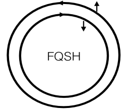
Figure 1: The fractional quantum spin Hall edge consists of two counter-propagating chiral Luttinger Liquids — one for each spin direction ($\uparrow,\downarrow$)

As discussed above, the edge theory for the $\nu=1/k$ fractional quantum spin Hall state consists of two chiral Luttinger liquids with opposite chiralities — one for each spin direction (Fig. 1). The purpose of this section is to review the Hamiltonian formulation of this edge theory.Wen (1995, 2007); Levin and Stern (2009) More specifically we will discuss the edge theory for a disk geometry where the circumference of the disk has length $L$. Since we will work in a Hamiltonian formulation, in order to define the edge theory we need to specify the Hamiltonian, the set of physical observables, and the canonical commutation relations.

We begin with the set of physical observables. The basic physical observables in the edge theory are a collection of operators $\{\partial_{y}\phi_{\uparrow}(y),\partial_{y}\phi_{\downarrow}(y)\}$ along with two additional operators $\phi_{\uparrow}(y_{0})$, $\phi_{\downarrow}(y_{0})$ where $y_{0}$ is an arbitrary, but fixed, point on the boundary of the disk. The $\{\partial_{y}\phi_{\uparrow}(y),\partial_{y}\phi_{\downarrow}(y),\phi_{\uparrow}(y_{0}),\phi_{\downarrow}(y_{0})\}$ operators can be thought of as the fundamental phase space operators in this system, i.e. the analogues of the $\{x_{1},...,x_{N},p_{1},...,p_{N}\}$ operators in section II. Like $\{x_{1},...,x_{N},p_{1},...,p_{N}\}$, all other physical observables can be written as functions/functionals of $\{\partial_{y}\phi_{\uparrow}(y),\partial_{y}\phi_{\downarrow}(y),\phi_{\uparrow}(y_{0}),\phi_{\downarrow}(y_{0})\}$. Two important examples are the operators $\phi_{\uparrow}(y)$ and $\phi_{\downarrow}(y)$ which are defined by

$$\phi_{\sigma}(y)\equiv\phi_{\sigma}(y_{0})+\int_{y_{0}}^{y}\partial_{x}\phi_{\sigma}dx,\quad\sigma=\uparrow,\downarrow$$ (27)

where the integral runs from $y_{0}$ to $y$ in the clockwise direction.

The physical meaning of these operators is as follows: the density of spin-up electrons at position $y$ is given by $\rho_{\uparrow}(y)=\frac{1}{2\pi}\partial_{y}\phi_{\uparrow}$ while the density of spin-down electron is $\rho_{\downarrow}(y)=\frac{1}{2\pi}\partial_{y}\phi_{\downarrow}$. The total charge $Q$ and total spin $S^{z}$ on the edge are given by $Q=Q_{\uparrow}+Q_{\downarrow}$ and $S^{z}=1/2(Q_{\uparrow}-Q_{\downarrow})$ with

$$Q_{\sigma}=\frac{1}{2\pi}\int_{-L/2}^{L/2}\partial_{y}\phi_{\sigma}dy,\quad\sigma=\uparrow,\downarrow$$

Finally, the spin-up and spin-down electron creation operators take the form

$$\psi_{\uparrow}^{\dagger}=e^{ik\phi_{\uparrow}},\quad\psi_{\downarrow}^{\dagger}=e^{-ik\phi_{\downarrow}}$$

In the above discussion, we ignored an important subtlety: $\phi_{\uparrow}(y_{0})$ and $\phi_{\downarrow}(y_{0})$ are actually compact degrees of freedom which are only defined modulo $2\pi/k$. In other words, strictly speaking, $\phi_{\uparrow}(y_{0})$ and $\phi_{\downarrow}(y_{0})$ are not well-defined operators: only $e^{ik\phi_{\uparrow}(y_{0})}$ and $e^{ik\phi_{\downarrow}(y_{0})}$ are well-defined. (Of course the same also goes for $\phi_{\uparrow}(y)$ and $\phi_{\downarrow}(y)$, in view of the above definition). Closely related to this fact, the conjugate “momenta” $Q_{\uparrow}$ and $Q_{\downarrow}$ are actually discrete degrees of freedom which can take only integer values.

The compactness of $\phi_{\uparrow}(y_{0}),\phi_{\downarrow}(y_{0})$ and discreteness of $Q_{\uparrow},Q_{\downarrow}$ is inconvenient for us since the machinery discussed in section II is designed for systems in which all the phase space operators are real-valued, rather than systems in which some operators are angular valued and some are integer valued. To get around this issue, we will initially treat $\phi_{\uparrow}(y_{0})$ and $\phi_{\downarrow}(y_{0})$ and the conjugate momenta $Q_{\uparrow}$, $Q_{\downarrow}$ as real valued operators. We will then use a trick (described in the next section) to dynamically generate the compactness of $\phi_{\uparrow}(y_{0}),\phi_{\downarrow}(y_{0})$ as well as the discreteness of $Q_{\uparrow},Q_{\downarrow}$.

Let us now discuss the commutation relations for the $\{\partial_{y}\phi_{\uparrow}(y),\partial_{y}\phi_{\downarrow}(y),\phi_{\uparrow}(y_{0}),\phi_{\downarrow}(y_{0})\}$ operators. Like the usual phase space operators $\{x_{1},...,x_{N},p_{1},...,p_{N}\}$, the commutators of $\{\partial_{y}\phi_{\uparrow}(y),\partial_{y}\phi_{\downarrow}(y),\phi_{\uparrow}(y_{0}),\phi_{\downarrow}(y_{0})\}$ are $c$-numbers. More specifically, the basic commutation relations are

$$[\partial_{x}\phi_{\uparrow}(x),\partial_{y}\phi_{\uparrow}(y)] =\frac{2\pi i}{k}\partial_{x}\delta(x-y)$$

$$[\partial_{x}\phi_{\downarrow}(x),\partial_{y}\phi_{\downarrow}(y)] =-\frac{2\pi i}{k}\partial_{x}\delta(x-y)$$

$$[\phi_{\uparrow}(y_{0}),\partial_{y}\phi_{\uparrow}(y)] =\frac{2\pi i}{k}\delta(y-y_{0})$$

$$[\phi_{\downarrow}(y_{0}),\partial_{y}\phi_{\downarrow}(y)] =-\frac{2\pi i}{k}\delta(y-y_{0})$$ (28)

with the other commutators vanishing:

$$[\phi_{\uparrow}(y_{0}),\partial_{y}\phi_{\downarrow}(y)] =[\phi_{\downarrow}(y_{0}),\partial_{y}\phi_{\uparrow}(y)]=0$$

$$[\phi_{\uparrow}(y_{0}),\phi_{\downarrow}(y_{0})] =[\partial_{x}\phi_{\uparrow}(x),\partial_{y}\phi_{\downarrow}(y)]=0$$

Using these basic commutation relations, together with the definition of $\phi_{\sigma}(y)$ (27), one can derive the more general relations

$$[\phi_{\uparrow}(x),\partial_{y}\phi_{\uparrow}(y)] =\frac{2\pi i}{k}\delta(x-y)$$

$$[\phi_{\downarrow}(x),\partial_{y}\phi_{\downarrow}(y)] =-\frac{2\pi i}{k}\delta(x-y)$$

$$[\phi_{\uparrow}(x),\partial_{y}\phi_{\downarrow}(y)] =0$$ (29)

as well as

$$[\phi_{\uparrow}(x),\phi_{\uparrow}(y)] =\frac{\pi i}{k}\text{sgn}(x,y)$$

$$[\phi_{\downarrow}(x),\phi_{\downarrow}(y)] =-\frac{\pi i}{k}\text{sgn}(x,y)$$

$$[\phi_{\uparrow}(x),\phi_{\downarrow}(y)] =0$$ (30)

where the sgn function is defined by $\text{sgn}(x,y)=+1$ if $y_{0}<x<y$ and $\text{sgn}(x,y)=-1$ if $y_{0}<y<x$, with the ordering defined in the clockwise direction. The latter commutation relations (29) and (30) will be particularly useful to us in the sections that follow.

Having defined the physical observables and their commutation relations, the last step is to define the Hamiltonian for the edge theory. The Hamiltonian for a perfectly clean, homogeneous edge is

$$H_{0}=\frac{kv}{4\pi}\int_{-L/2}^{L/2}[(\partial_{x}\phi_{\uparrow}(x))^{2}+(\partial_{x}\phi_{\downarrow}(x))^{2}]dx$$ (31)

where $v$ is the velocity of the edge modes.

At this point, the edge theory is complete except for one missing element: we have not given an explicit definition of the Hilbert space of the edge theory. There are two different (but equivalent) definitions that one can use. The first, more abstract, definition is that the Hilbert space is the unique irreducible representation of the operators $\{\partial_{y}\phi_{\uparrow},\partial_{y}\phi_{\downarrow},\phi_{\uparrow}(y_{0}),\phi_{\downarrow}(y_{0})\}$ and the commutation relations (28). (This is akin to defining the Hilbert space of the 1D harmonic oscillator as the irreducible representation of the Heisenberg algebra $[x,p]=i$). The second definition, which is more concrete but also more complicated, is that the Hilbert space is spanned by the complete orthonormal basis $\{|q_{\uparrow},q_{\downarrow},\{n_{p\uparrow}\},\{n_{p\downarrow}\}\rangle\}$ where the quantum numbers $q_{\uparrow},q_{\downarrow}$ range over all integers while $n_{p\uparrow},n_{p\downarrow}$ range over all nonnegative integers for each value of $p=2\pi/L,4\pi/L,...$. These basis states have a simple physical meaning: $|q_{\uparrow},q_{\downarrow},\{n_{p\uparrow}\},\{n_{p\downarrow}\}\rangle$ corresponds to a state with charge $q_{\uparrow}$ and $q_{\downarrow}$ on the two edge modes, and with $n_{p\uparrow}$ and $n_{p\downarrow}$ phonons with momentum $p$ on the two edge modes.

III.2 Example 1: Single magnetic impurity

With this preparation, we now proceed to study a fractional quantum spin Hall edge with a single magnetic impurity in a disk geometry of circumference $L$ (Fig. 2a). We assume that the impurity, which is located at $x=0$, generates a backscattering term of the form $\frac{U}{2}(\psi_{\uparrow}^{\dagger}(0)\psi_{\downarrow}(0)+h.c)$. Thus, in the bosonized language, the system with an impurity is described by the Hamiltonian

$$H=H_{0}-U\cos(C),\quad C=k(\phi_{\uparrow}(0)+\phi_{\downarrow}(0))$$ (32)

where $H_{0}$ is defined in Eq. 31. Here, we temporarily ignore the question of how we regularize the cosine term; we will come back to this point below.

Our goal is to find the low energy spectrum of $H$ in the strong backscattering limit, $U\rightarrow\infty$. We will accomplish this using the results from section II. Note that, in using these results, we implicitly assume that our formalism applies to systems with infinite dimensional phase spaces, even though we only derived it in the finite dimensional case.

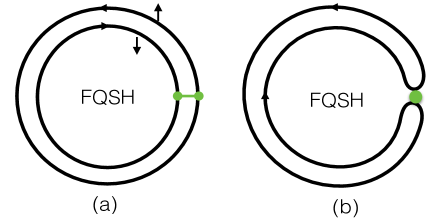
Figure 2: (a) A magnetic impurity on a fractional quantum spin Hall edge causes spin-up electrons to backscatter into spin-down electrons. (b) In the infinite backscattering limit, the impurity effectively reconnects the edge modes.

First we describe a trick for correctly accounting for the compactness of $\phi_{\uparrow}(y_{0}),\phi_{\downarrow}(y_{0})$ and the quantization of $Q_{\uparrow},Q_{\downarrow}$. The idea is simple: we initially treat these variables as if they are real valued, and then we introduce compactness dynamically by adding two additional cosine terms to our Hamiltonian:

$$H=H_{0}-U\cos(C)-U\cos(2\pi Q_{\uparrow})-U\cos(2\pi Q_{\downarrow})$$ (33)

These additional cosine terms effectively force $Q_{\uparrow}$ and $Q_{\downarrow}$ to be quantized at low energies, thereby generating the compactness that we seek. We will include all three cosine terms in our subsequent analysis.

The next step is to calculate the low energy effective Hamiltonian $H_{\text{eff}}$ and low energy Hilbert space $\mathcal{H}_{\text{eff}}$. Instead of working out the expressions in Eqs. 2, 5, we will skip this computation and proceed directly to finding creation and annihilation operators for $H_{\text{eff}}$ using Eq. 11. (This approach works because equation (11) does not require us to find the explicit form of $H_{\text{eff}}$).

According to Eq. 11, we can find the creation and annihilation operators for $H_{\text{eff}}$ by finding all operators $a$ such that (1) $a$ is a linear combination of our fundamental phase space operators $\{\partial_{y}\phi_{\uparrow},\partial_{y}\phi_{\downarrow},\phi_{\uparrow}(y_{0}),\phi_{\downarrow}(y_{0})\}$ and (2) $a$ obeys

$$[a,H_{0}] =Ea+\lambda[C,H_{0}]+\lambda_{\uparrow}[Q_{\uparrow},H_{0}]+\lambda_{\downarrow}[Q_{\downarrow},H_{0}]$$

$$[a,C] =[a,Q_{\uparrow}]=[a,Q_{\downarrow}]=0$$ (34)

for some scalars $E,\lambda,\lambda_{\uparrow},\lambda_{\downarrow}$ with $E\neq 0$.

To proceed further, we note that the constraint $[a,Q_{\uparrow}]=[a,Q_{\downarrow}]=0$, implies that $\phi_{\uparrow}(y_{0}),\phi_{\downarrow}(y_{0})$ cannot appear in the expression for $a$. Hence, $a$ can be written in the general form

$$a=\int_{-L/2}^{L/2}[f_{\uparrow}(y)\partial_{y}\phi_{\uparrow}(y)+f_{\downarrow}(y)\partial_{y}\phi_{\downarrow}(y)]dy$$ (35)

Substituting this expression into the first line of Eq. 34 we obtain the differential equations

$$-ivf_{\uparrow}^{\prime}(y) =Ef_{\uparrow}(y)+\lambda kiv\delta(y)$$

$$ivf_{\downarrow}^{\prime}(y) =Ef_{\downarrow}(y)-\lambda kiv\delta(y)$$

(The $\lambda_{\uparrow},\lambda_{\downarrow}$ terms drop out of these equations since $Q_{\uparrow},Q_{\downarrow}$ commute with $H_{0}$). These differential equations can be solved straightforwardly. The most general solution takes the form

$$f_{\uparrow}(y) =e^{ipy}[A_{1}\Theta(-y)+A_{2}\Theta(y)]$$

$$f_{\downarrow}(y) =e^{-ipy}[B_{1}\Theta(-y)+B_{2}\Theta(y)]$$ (36)

where $p=E/v$, and

$$A_{2}=A_{1}-\lambda k,B_{2}=B_{1}-\lambda k$$ (37)

Here $\Theta$ is the Heaviside step function defined as

$$\Theta(x)=\begin{cases}0&-L/2\leq x\leq 0\\ 1&0\leq x\leq L/2\end{cases}$$

(Note that the above expressions (36) for $f_{\uparrow},f_{\downarrow}$ do not obey periodic boundary conditions at $x=\pm L/2$; we will not impose these boundary conditions until later in our calculation). Eliminating $\lambda$ from (37) we see that

$$A_{2}-A_{1}=B_{2}-B_{1}$$ (38)

We still have to impose one more condition on $a$, namely $[a,C]=0$. This condition leads to a second constraint on $A_{1},A_{2},B_{1},B_{2}$, but the derivation of this constraint is somewhat subtle. The problem is that if we simply substitute (35) into $[a,C]=0$, we find

$$f_{\uparrow}(0)=f_{\downarrow}(0)$$ (39)

It is unclear how to translate this relation into one involving $A_{1},A_{2},B_{1},B_{2}$ since $f_{\uparrow},f_{\downarrow}$ are discontinuous at $x=0$ and hence $f_{\uparrow}(0),f_{\downarrow}(0)$ are ill-defined. The origin of this puzzle is that the cosine term in Eq. 32 contains short-distance singularities and hence is not well-defined. To resolve this issue we regularize the argument of the cosine term, replacing $C=k(\phi_{\uparrow}(0)+\phi_{\downarrow}(0))$ with

$$C\rightarrow\int_{-L/2}^{L/2}k(\phi_{\uparrow}(x)+\phi_{\downarrow}(x))\tilde{\delta}(x)dx$$ (40)

where $\tilde{\delta}$ is a narrowly peaked function with $\int\tilde{\delta}(x)dx=1$. Here, we can think of $\tilde{\delta}$ as an approximation to a delta function. Note that $\tilde{\delta}$ effectively introduces a short-distance cutoff and thus makes the cosine term non-singular. After making this replacement, it is straightforward to repeat the above analysis and solve the differential equations for $f_{\uparrow},f_{\downarrow}$. In appendix G, we work out this exercise, and we find that with this regularization, the condition $[a,C]=0$ leads to the constraint

$$\frac{A_{1}+A_{2}}{2}=\frac{B_{1}+B_{2}}{2}$$ (41)

Combining our two constraints on $A_{1},B_{1},A_{2},B_{2}$ (38,41), we obtain the relations

$$A_{1}=B_{1},\quad A_{2}=B_{2}$$ (42)

So far we have not imposed any restriction on the momentum $p$. The momentum constraints come from the periodic boundary conditions on $f_{\uparrow},f_{\downarrow}$:

$$f_{\uparrow}(-L/2)=f_{\uparrow}(L/2),\quad f_{\downarrow}(-L/2)=f_{\downarrow}(L/2)$$

Using the explicit form of $f_{\uparrow},f_{\downarrow}$, these boundary conditions give

$$A_{1}e^{-ipL/2}=A_{2}e^{ipL/2},\quad B_{1}e^{ipL/2}=B_{2}e^{-ipL/2}$$

from which we deduce

$$e^{2ipL}=1,\quad A_{2}=A_{1}e^{-ipL}$$ (43)

Putting this all together, we see that the most general possible creation/annihilation operator for $H_{\text{eff}}$ is given by

$$a_{p}=A_{1}\int_{-L/2}^{L/2} (e^{ipy}\partial_{y}\phi_{\uparrow}+e^{-ipy}\partial_{y}\phi_{\downarrow})\Theta(-y)$$

$$+e^{-ipL} (e^{ipy}\partial_{y}\phi_{\uparrow}+e^{-ipy}\partial_{y}\phi_{\downarrow})\Theta(y)dy$$

where $p$ is quantized as $p=\pm\pi/L,\pm 2\pi/L,...$ and $E_{p}=vp$. (Note that $p=0$ does not correspond to a legitimate creation/annihilation operator according to the definition given above, since we require $E\neq 0$).

Following the conventions from section II.2, we will refer to the operators with $E_{p}>0$ — or equivalently $p>0$ — as “annihilation operators” and the other operators as “creation operators.” Also, we will choose the normalization constant $A_{1}$ so that $[a_{p},a_{p^{\prime}}^{\dagger}]=\delta_{pp^{\prime}}$ for $p,p^{\prime}>0$. This gives the expression

$$a_{p}=\sqrt{\frac{k}{4\pi|p|L}}\int_{-L/2}^{L/2} (e^{ipy}\partial_{y}\phi_{\uparrow}+e^{-ipy}\partial_{y}\phi_{\downarrow})\Theta(-y)$$

$$+e^{-ipL} (e^{ipy}\partial_{y}\phi_{\uparrow}+e^{-ipy}\partial_{y}\phi_{\downarrow})\Theta(y)dy$$ (44)

The next step is to compute the commutator matrix $\mathcal{Z}_{ij}$. In the case at hand, we have three cosine terms $\{\cos(C_{1}),\cos(C_{2}),\cos(C_{3})\}$, where

$$C_{1}=C,\quad C_{2}=2\pi Q_{\uparrow},\quad C_{3}=2\pi Q_{\downarrow}$$

Therefore $\mathcal{Z}_{ij}$ is given by

$$\mathcal{Z}_{ij}=\frac{1}{2\pi i}[C_{i},C_{j}]=\begin{pmatrix}0&1&-1\\ -1&0&0\\ 1&0&0\end{pmatrix}$$

To proceed further we need to find an appropriate change of variables of the form $C_{i}^{\prime}=\sum_{j=1}^{3}\mathcal{V}_{ij}C_{j}+\chi_{i}$. Here, $\mathcal{V}$ should an integer matrix with determinant $\pm 1$ with the property that $\mathcal{Z}_{ij}^{\prime}=\frac{1}{2\pi i}[C_{i}^{\prime},C_{j}^{\prime}]$ is in skew-normal form, while $\chi$ should be a real vector satisfying Eq. 15. It is easy to see that the following change of variables does the job:

$$C_{1}^{\prime}=C_{1},\quad C_{2}^{\prime}=-2\pi Q_{\uparrow},\quad C_{3}^{\prime}=2\pi Q_{\uparrow}+2\pi Q_{\downarrow}$$

Indeed, for this change of variables,

$$\mathcal{Z}^{\prime}=\begin{pmatrix}0&-1&0\\ 1&0&0\\ 0&0&0\end{pmatrix}$$

We can see that this is in the canonical skew normal form shown in Eq. 14, with the parameters $M=3$, $I=1$, $d_{1}=1$.

We are now in a position to write down the low energy effective Hamiltonian $H_{\text{eff}}$: according to Eq. 16, $H_{\text{eff}}$ must take the form

$$H_{\text{eff}}=\sum_{p>0}vpa_{p}^{\dagger}a_{p}+F\cdot(C_{3}^{\prime})^{2}$$ (45)

where $F$ is some (as yet unknown) constant. To determine the constant $F$, we make two observations. First, we note that the first term in Eq. 45 can be rewritten as $\sum_{p\neq 0}\frac{v|p|}{2}(a_{-p}a_{p})$. Second, we note that $C_{3}^{\prime}=2\pi Q$ is proportional to $a_{p=0}$. Given these observations, it is natural to interpret the $F(C_{3}^{\prime})^{2}$ term as the missing $p=0$ term in the sum. This suggests that we can fix the coefficient $F$ using continuity in the $p\rightarrow 0$ limit. To this end, we observe that

$$\lim_{p\rightarrow 0}\frac{v|p|}{2}a_{-p}a_{p}=\frac{vk}{8\pi L}\cdot(C_{3}^{\prime})^{2}$$

We conclude that $F=\frac{vk}{8\pi L}$. Substituting this into (45), we derive

$$H_{\text{eff}}=\sum_{p>0}vpa_{p}^{\dagger}a_{p}+\frac{vk}{8\pi L}\cdot(C_{3}^{\prime})^{2}$$ (46)

where the sum runs over $p=\pi/L,2\pi/L,...$.

In addition to the effective Hamiltonian, we also need to discuss the effective Hilbert space $\mathcal{H}_{\text{eff}}$ in which this Hamiltonian is defined. According to the results of section II.2, the effective Hilbert space $\mathcal{H}_{\text{eff}}$ is spanned by states $\{|q,\{n_{p}\}\rangle\}$ where $|q,\{n_{p}\}\rangle$ is the unique simultaneous eigenstate of the form

$$e^{iC_{1}^{\prime}}|q,\{n_{p}\}\rangle =|q,\{n_{p}\}\rangle,$$

$$e^{iC_{2}^{\prime}}|q,\{n_{p}\}\rangle =|q,\{n_{p}\}\rangle,$$

$$C_{3}^{\prime}|q,\{n_{p}\}\rangle =2\pi q|q,\{n_{p}\}\rangle,$$

$$a_{p}^{\dagger}a_{p}|q,\{n_{p}\}\rangle =n_{p}|q,\{n_{p}\}\rangle$$

Here $n_{p}$ runs over non-negative integers, while $q$ runs over all integers. Note that we do not need to label the $\{|q,\{n_{p}\}\rangle\}$ basis states with $\alpha$ quantum numbers since $d_{1}=1$ so there is no degeneracy.

Having derived the effective theory, all that remains is to diagonalize it. Fortunately we can accomplish this without any extra work: from (46) it is clear that the $\{|q,\{n_{p}\}\rangle\}$ basis states are also eigenstates of $H_{\text{eff}}$ with energies given by

$$E=\sum_{p>0}vpn_{p}+\frac{\pi vk}{2L}\cdot q^{2}$$ (47)

We are now finished: the above equation gives the complete energy spectrum of $H_{\text{eff}}$, and thus the complete low energy spectrum of $H$ in the limit $U\rightarrow\infty$.

To understand the physical interpretation of this energy spectrum, we can think of $n_{p}$ as describing the number of phonon excitations with momentum $p$, while $q$ describes the total charge on the edge. With these identifications, the first term in (47) describes the total energy of the phonon excitations — which are linearly dispersing with velocity $v$ — while the second term describes the charging/capacitative energy of the edge.

It is interesting that at low energies, our system has only one branch of phonon modes and one charge degree of freedom, while the clean edge theory (31) has two branches of phonon modes and two charge degrees of freedom — one for each spin direction. The explanation for this discrepancy can be seen in Fig. 2b: in the infinite $U$ limit, the impurity induces perfect backscattering which effectively reconnects the edges to form a single chiral edge of length $2L$.

III.3 Example 2: Multiple magnetic impurities

We now consider a fractional quantum spin Hall edge in a disk geometry with $N$ magnetic impurities located at positions $x_{1},...,x_{N}$ (Fig. 3a). Modeling the impurities in the same way as in the previous section, the Hamiltonian is

$$H=H_{0}-U\sum_{i=1}^{N}\cos(C_{i}),\quad C_{i}=k(\phi_{\uparrow}(x_{i})+\phi_{\downarrow}(x_{i}))$$ (48)

where $H_{0}$ is defined in Eq. 31.

As in the single impurity case, our goal is to understand the low energy physics of $H$ in the limit $U\rightarrow\infty$. We can accomplish this using the same approach as before. The first step is to take account of the compactness of $\phi_{\uparrow},\phi_{\downarrow}$ and the discrete nature of $Q_{\uparrow},Q_{\downarrow}$ by adding two additional cosine terms to our Hamiltonian:

$$H=H_{0}-U\sum_{i=1}^{N}\cos(C_{i})-U\cos(2\pi Q_{\uparrow})-U\cos(2\pi Q_{\downarrow})$$

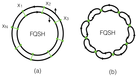
Figure 3: (a) A collection of $N$ magnetic impurities on a fractional quantum spin Hall edge. The impurities are located at positions $x_{1},...,x_{N}$. (b) In the infinite backscattering limit, the impurities effectively reconnect the edge modes, breaking the edge into $N$ disconnected components.

Next, we find the creation and annihilation operators for $H_{\text{eff}}$ using Eq. 11. That is, we search for all operators $a$ such that (1) $a$ is a linear combination of our fundamental phase space operators $\{\partial_{y}\phi_{\uparrow},\partial_{y}\phi_{\downarrow},\phi_{\uparrow}(y_{0}),\phi_{\downarrow}(y_{0})\}$ and (2) $a$ obeys

$$[a,H_{0}] =Ea+\sum_{i=1}^{N}\lambda_{i}[C_{i},H_{0}]+\lambda_{\uparrow}[Q_{\uparrow},H_{0}]+\lambda_{\downarrow}[Q_{\downarrow},H_{0}]$$

$$[a,C_{j}] =[a,Q_{\uparrow}]=[a,Q_{\downarrow}]=0$$ (49)

for some $E,{\color[rgb]{0,0,0}\lambda_{i}},\lambda_{\uparrow},\lambda_{\downarrow}$ with $E\neq 0$.

Given that $[a,Q_{\uparrow}]=[a,Q_{\downarrow}]=0$, we know that $\phi_{\uparrow}(y_{0}),\phi_{\downarrow}(y_{0})$ cannot appear in the expression for $a$. Hence, $a$ can be written in the general form

$$a=\int_{-L/2}^{L/2}[f_{\uparrow}(y)\partial_{y}\phi_{\uparrow}(y)+f_{\downarrow}(y)\partial_{y}\phi_{\downarrow}(y)]dy$$

Substituting these expressions into the first line of Eq. 49, we obtain

$$-ivf_{\uparrow}^{\prime}(y) =Ef_{\uparrow}(y)+kiv\sum_{j=1}^{N}\lambda_{j}\delta(y-x_{j})$$

$$ivf_{\downarrow}^{\prime}(y) =Ef_{\downarrow}(y)-kiv\sum_{j=1}^{N}\lambda_{j}\delta(y-x_{j})$$

Solving these differential equations gives

$$f_{\uparrow}(y) =\sum_{j=1}^{N}A_{j}e^{ipy}\Theta(x_{j-1}<y<x_{j})]$$

$$f_{\downarrow}(y) =\sum_{j=1}^{N}B_{j}e^{-ipy}\Theta(x_{j-1}<y<x_{j})]$$

where $p=E/v$ and where

$$A_{j+1}=A_{j}-\lambda_{j}ke^{-ipx_{j}},\quad B_{j+1}=B_{j}-\lambda_{j}ke^{ipx_{j}}$$

Here, $\Theta(a<y<b)$ is defined to take the value $1$ if $y$ is in the interval $[a,b]$ and $0$ otherwise. Also, we use a notation in which $x_{0}$ is identified with $x_{N}$. Eliminating $\lambda_{j}$, we derive

$$(A_{j+1}-A_{j})e^{ipx_{j}}=(B_{j+1}-B_{j})e^{-ipx_{j}}$$ (50)

We still have to impose the condition $[a,C_{j}]=0$, which gives an additional set of constraints on $\{A_{j},B_{j}\}$. As in the single impurity case, we regularize the cosine terms to derive these constraints. That is, we replace $C=k(\phi_{\uparrow}(x_{j})+\phi_{\downarrow}(x_{j}))$ with

$$C\rightarrow\int_{-L/2}^{L/2}k(\phi_{\uparrow}(x)+\phi_{\downarrow}(x))\tilde{\delta}(x-x_{j})dx$$ (51)

where $\tilde{\delta}$ is a narrowly peaked function with $\int\tilde{\delta}(x)dx=1$, i.e., an approximation to a delta function. With this regularization, it is not hard to show that $[a,C_{j}]=0$ gives the constraint

$$\frac{1}{2}(A_{j}+A_{j+1})e^{ipx_{j}}=\frac{1}{2}(B_{j}+B_{j+1})e^{-ipx_{j}}$$ (52)

Combining (50), (52) we derive

$$A_{j}e^{ipx_{j}}=B_{j}e^{-ipx_{j}},\quad A_{j+1}e^{ipx_{j}}=B_{j+1}e^{-ipx_{j}}$$ (53)

Our task is now to find all $\{A_{j},B_{j},p\}$ that satisfy (53). For simplicity, we will specialize to the case where the impurities are uniformly spaced with spacing $s$, i.e. $x_{j+1}-x_{j}=s=L/N$ for all $j$. In this case, equation (53) implies that $e^{2ips}=1$, so that $p$ is quantized in integer multiples of $\pi/s$. For any such $p$, (53) has $N$ linearly independent solutions of the form

$$B_{j} =A_{j}=0\ \ \text{for }j\neq m$$

$$B_{j} =A_{j}e^{2ipx_{j}}\neq 0\ \ \text{for }j=m$$

with $m=1,...,N$. Putting this all together, we see that the most general possible creation/annihilation operator for $H_{\text{eff}}$ is given by

$$a_{pm}=\sqrt{\frac{k}{4\pi|p|s}}\int_{-L/2}^{L/2} [(e^{ipy}\partial_{y}\phi_{\uparrow}+e^{2ipx_{m}}e^{-ipy}\partial_{y}\phi_{\downarrow})$$

$$\cdot\Theta(x_{m-1}<y<x_{m})]dy$$

with $E_{pm}=vp$. Here the index $m$ runs over $m=1,...,N$ while $p$ takes values $\pm\pi/s,\pm 2\pi/s,...$. (As in the single impurity case, $p=0$ does not correspond to a legitimate creation/annihilation operator, since we require that $E\neq 0$).

Following the conventions from section II.2, we will refer to the operators with $E>0$ — or equivalently $p>0$ — as “annihilation operators” and the other operators as “creation operators.” Note that we have normalized the $a$ operators so that $[a_{pm},a_{p^{\prime}m^{\prime}}^{\dagger}]=\delta_{pp^{\prime}}\delta_{mm^{\prime}}$ for $p,p^{\prime}>0$.

The next step is to compute the commutator matrix $\mathcal{Z}_{ij}=\frac{1}{2\pi i}[C_{i},C_{j}]$. Let us denote the $N+2$ cosine terms as $\{\cos(C_{1}),...,\cos(C_{N+2})\}$ where $C_{N+1}=2\pi Q_{\uparrow}$, $C_{N+2}=2\pi Q_{\downarrow}$. Using (30) we find that $\mathcal{Z}_{ij}$ takes the form

$$\mathcal{Z}_{ij} = \begin{pmatrix}0&\cdots&0&1&-1\\ \vdots&\vdots&\vdots&\vdots&\vdots\\ 0&\cdots&0&1&-1\\ -1&\cdots&-1&0&0\\ 1&\cdots&1&0&0\end{pmatrix}$$

To proceed further we need to find an appropriate change of variables of the form $C_{i}^{\prime}=\sum_{j=1}^{N+2}\mathcal{V}_{ij}C_{j}+\chi_{i}$. Here, $\mathcal{V}$ should be chosen so that $\mathcal{Z}_{ij}^{\prime}=\frac{1}{2\pi i}[C_{i}^{\prime},C_{j}^{\prime}]$ is in skew-normal form, while $\chi$ should be chosen so that it obeys Eq. 15. It is easy to see that the following change of variables does the job:

$$C_{1}^{\prime}=C_{1},\quad C_{2}^{\prime}=-2\pi Q_{\uparrow},\quad C_{3}^{\prime}=2\pi Q_{\uparrow}+2\pi Q_{\downarrow}$$

$$C_{m}^{\prime}=C_{m-2}-C_{m-3},\quad m=4,...,N+2$$

Indeed, it is easy to check that

$$\mathcal{Z}_{ij}^{\prime} = \frac{1}{2\pi i}[C_{i}^{\prime},C_{j}^{\prime}]$$

$$= \begin{pmatrix}0&-1&0&\cdots&0\\ 1&0&0&\cdots&0\\ 0&0&0&\cdots&0\\ \vdots&\vdots&\vdots&\vdots&\vdots\\ 0&0&0&\cdots&0\end{pmatrix}$$

We can see that this is in the canonical skew-normal form shown in Eq. 14, with the parameters $M=N+2$, $I=1$, $d_{1}=1$.

We are now in a position to write down the low energy effective Hamiltonian $H_{\text{eff}}$: according to Eq. 16, $H_{\text{eff}}$ must take the form

$$H_{\text{eff}}=\sum_{m=1}^{N}\sum_{p>0}vpa_{pm}^{\dagger}a_{pm}+F(C_{3}^{\prime},...,C_{N+2}^{\prime})$$ (54)

where the sum runs over $p=\pi/s,2\pi/s,...$ and where $F$ is some quadratic function of $N$ variables. To determine $F$, we first need to work out more concrete expressions for $C_{m}^{\prime}$. The $m=3$ case is simple: $C_{3}^{\prime}=2\pi Q$. On the other hand, for $m=4,...,N+2$, we have

$$C_{m}^{\prime} = k(\phi_{\uparrow}(x_{m-2})+\phi_{\downarrow}(x_{m-2}))$$

$$- k(\phi_{\uparrow}(x_{m-3})+\phi_{\downarrow}(x_{m-3})$$

$$= k\int_{x_{m-3}}^{x_{m-2}}(\partial_{y}\phi_{\uparrow}+\partial_{y}\phi_{\downarrow})dy$$

where the second line follows from the definition of $\phi_{\uparrow},\phi_{\downarrow}$ (27) along with the assumption that the impurities are arranged in the order $y_{0}<x_{1}<...<x_{N}$ in the clockwise direction.

With these expressions we can now find $F$. We use the same trick as in the single impurity case: we note that the first term in Eq. 54 can be rewritten as as $\sum_{m}\sum_{p\neq 0}\frac{v|p|}{2}(a_{-pm}a_{pm})$, and we observe that

$$\lim_{p\rightarrow 0}\frac{v|p|}{2}a_{-pm}a_{pm}=\frac{v}{8\pi ks}\cdot(C_{m+2}^{\prime})^{2}$$

for $m=2,...,N$, while

$$\lim_{p\rightarrow 0}\frac{v|p|}{2}a_{-p1}a_{p1}=\frac{v}{8\pi ks}\cdot(kC_{3}^{\prime}-\sum_{m=4}^{N+2}C_{m^{\prime}})^{2}$$

Assuming that $F$ reproduces the missing $p=0$ piece of the first term in Eq. 54, we deduce that

$$F(C_{3}^{\prime},...,C_{N+2}^{\prime}) = \frac{v}{8\pi ks}\cdot\sum_{m=4}^{N+2}(C_{m}^{\prime})^{2}$$ (55)

$$+ \frac{v}{8\pi ks}\cdot(kC_{3}^{\prime}-\sum_{m=4}^{N+2}C_{m}^{\prime})^{2}$$

In addition to the effective Hamiltonian, we also need to discuss the effective Hilbert space $\mathcal{H}_{\text{eff}}$. Applying the results of section II.2, we see that $\mathcal{H}_{\text{eff}}$ is spanned by states $\{|\boldsymbol{q},\{n_{pm}\}\rangle\}$ where $|\boldsymbol{q},\{n_{pm}\}\rangle$ is the unique simultaneous eigenstate of the form

$$e^{iC_{1}^{\prime}}|\boldsymbol{q},\{n_{pm}\}\rangle =|\boldsymbol{q},\{n_{pm}\}\rangle,$$

$$e^{iC_{2}^{\prime}}|\boldsymbol{q},\{n_{pm}\}\rangle =|\boldsymbol{q},\{n_{pm}\}\rangle,$$

$$C_{i}^{\prime}|\boldsymbol{q},\{n_{pm}\}\rangle =2\pi q_{i-2}|\boldsymbol{q},\{n_{pm}\}\rangle,\ i=3,...,N+2$$

$$a_{pm}^{\dagger}a_{pm}|\boldsymbol{q},\{n_{pm}\}\rangle =n_{pm}|\boldsymbol{q},\{n_{pm}\}\rangle$$

Here $n_{pm}$ runs over non-negative integers, while $\boldsymbol{q}$ is an $N$ component vector, $\boldsymbol{q}=(q_{1},...,q_{N})$ where each component $q_{i}$ runs over all integers. As in the single impurity case, we do not need to label the $\{|\boldsymbol{q},\{n_{pm}\}\rangle\}$ basis states with $\alpha$ quantum numbers since $d_{1}=1$ and thus there is no degeneracy.

Now that we have derived the effective theory, all that remains is to diagonalize it. To do this, we note that the $\{|\boldsymbol{q},\{n_{pm}\}\rangle\}$ basis states are also eigenstates of $H_{\text{eff}}$ with energies given by

$$E=\sum_{m=1}^{N}\sum_{p>0}vpn_{pm} + \frac{\pi v}{2ks}\sum_{m=2}^{N}q_{m}^{2}$$

$$+ \frac{\pi v}{2ks}(kq_{1}-q_{2}-...-q_{N})^{2}$$

The above equation gives the complete low energy spectrum of $H$ in the limit $U\rightarrow\infty$.

Let us now discuss the physical interpretation of these results. As in the single impurity case, when $U\rightarrow\infty$ the impurities generate perfect backscattering, effectively reconnecting the edge modes. The result, as shown in Fig. 3b, is the formation of $N$ disconnected chiral modes living in the $N$ intervals, $[x_{N},x_{1}],[x_{1},x_{2}],...,[x_{N-1},x_{N}]$.

With this picture in mind, the $n_{pm}$ quantum numbers have a natural interpretation as the number of phonon excitations with momentum $p$ on the $m$th disconnected component of the edge. Likewise, if we examine the definition of $q_{m}$, we can see that $q_{m}/k$ is equal to the total charge in the $m$th component of the edge, i.e. the total charge in the interval $[x_{m-1},x_{m}]$, for $m=2,...,N$. On the other hand, the quantum number $q_{1}$ is slightly different: $q_{1}$ is equal to the total charge on the entire boundary of the disk $[-L/2,L/2]$. Note that since $q_{m}$ is quantized to be an integer for all $m=1,...,N$, it follows that the charge in each interval $[x_{m-1},x_{m}]$ is quantized in integer multiples of $1/k$ while the total charge on the whole edge is quantized as an integer. These quantization laws are physically sensible: indeed, the fractional quantum spin Hall state supports quasiparticle excitations with charge $1/k$, so it makes sense that disconnected components of the edge can carry such charge, but at the same time we also know that the total charge on the boundary must be an integer.

Putting this all together, we see that the first term in (III.3) can be interpreted as the energy of the phonon excitations, summed over all momenta and all disconnected components of the edge. Similarly the second term can be interpreted as the charging energy of the disconnected components labeled by $m=2,...,N$, while the third term can be interpreted as the charging energy of the first component labeled by $m=1$.

So far in this section we have considered magnetic impurities which backscatter spin-up electrons into spin-down electrons. These impurities explicitly break time reversal symmetry. However, one can also consider non-magnetic impurities which preserve time reversal symmetry and backscatter pairs of spin-up electrons into pairs of spin-down electrons. When the scattering strength $U$ is sufficiently strong these impurities can cause a spontaneous breaking of time reversal symmetry, leading to a two-fold degenerate ground state. Xu and Moore (2006); Wu et al. (2006); Levin and Stern (2009) This physics can also be captured by an appropriate toy model and we provide an example in Appendix H.

III.4 Example 3: Multiple magnetic and superconducting impurities

We now consider a fractional quantum spin Hall edge in a disk geometry of circumference $L$ with $2N$ alternating magnetic and superconducting impurities. We take the magnetic impurities to be located at positions $x_{1},x_{3},...,x_{2N-1}$ while the superconducting impurities are located at positions $x_{2},x_{4},...,x_{2N}$ (Fig. 4a). We assume that the magnetic impurities generate a backscattering term of the form $\frac{U}{2}(\psi_{\uparrow}^{\dagger}(0)\psi_{\downarrow}(0)+h.c)$, while the superconducting impurities generate a pairing term of the form $\frac{U}{2}(\psi_{\uparrow}^{\dagger}(0)\psi_{\downarrow}^{\dagger}(0)+h.c)$. The Hamiltonian is then

$$H=H_{0}-U\sum_{i=1}^{2N}\cos(C_{i})$$ (57)

$$C_{i}=k(\phi_{\uparrow}(x_{i})+(-1)^{i+1}\phi_{\downarrow}(x_{i}))$$ (58)

where $H_{0}$ is defined in Eq. 31.

As in the previous cases, our goal is to understand the low energy physics of $H$ in the limit $U\rightarrow\infty$. As before, we take account of the compactness of $\phi_{\uparrow},\phi_{\downarrow}$ and the discrete nature of $Q_{\uparrow},Q_{\downarrow}$ by adding two additional cosine terms to our Hamiltonian:

$$H=H_{0}-U\sum_{i=1}^{2N}\cos(C_{i})-U\cos(2\pi Q_{\uparrow})-U\cos(2\pi Q_{\downarrow})$$ (59)

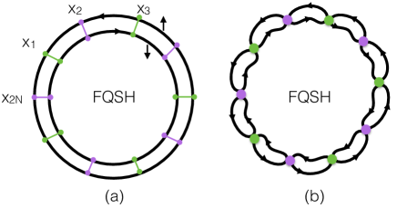
Figure 4: (a) A collection of $2N$ alternating magnetic and superconducting impurities on a fractional quantum spin Hall edge. The magnetic impurities are located at positions $x_{1},x_{3},....,x_{2N-1}$ while the superconducting impurities are located at positions $x_{2},x_{4},...,x_{2N}$. The magnetic impurities scatter spin-up electrons into spin-down electrons while the superconducting impurities scatter spin-up electrons into spin-down holes. (b) In the infinite $U$ limit, the impurities effectively reconnect the edge modes, breaking the edge into $2N$ disconnected components.

Next, we find the creation and annihilation operators for $H_{\text{eff}}$ using Eq. 11. That is, we search for all operators $a$ such that (1) $a$ is a linear combination of our fundamental phase space operators $\{\partial_{y}\phi_{\uparrow},\partial_{y}\phi_{\downarrow},\phi_{\uparrow}(y_{0}),\phi_{\downarrow}(y_{0})\}$ and (2) $a$ obeys

$$[a,H_{0}] =Ea+\sum_{i=1}^{2N}\lambda_{i}[C_{i},H_{0}]+\lambda_{\uparrow}[Q_{\uparrow},H_{0}]+\lambda_{\downarrow}[Q_{\downarrow},H_{0}]$$

$$[a,C_{j}] =[a,Q_{\uparrow}]=[a,Q_{\downarrow}]=0$$ (60)

for some $E,{\color[rgb]{0,0,0}\lambda_{i}},\lambda_{\uparrow},\lambda_{\downarrow}$ with $E\neq 0$.

As before, since $[a,Q_{\uparrow}]=[a,Q_{\downarrow}]=0$, it follows that $\phi_{\uparrow}(y_{0}),\phi_{\downarrow}(y_{0})$ cannot appear in the expression for $a$. Hence, $a$ can be written in the general form

$$a=\int_{-L/2}^{L/2}[f_{\uparrow}(y)\partial_{y}\phi_{\uparrow}(y)+f_{\downarrow}(y)\partial_{y}\phi_{\downarrow}(y)]dy$$

Substituting this expression into the first line of Eq. 60, we obtain

$$-ivf_{\uparrow}^{\prime}(y) =Ef_{\uparrow}+kiv\sum_{j}\lambda_{j}\delta(y-x_{j})$$

$$ivf_{\downarrow}^{\prime}(y) =Ef_{\downarrow}-kiv\sum_{j}(-1)^{j+1}\lambda_{j}\delta(y-x_{j})$$

Solving the above first order differential equation we get

$$f_{\uparrow}(y) =\sum_{j=1}^{N}A_{j}e^{ipy}\Theta(x_{j-1}<y<x_{j})]$$

$$f_{\downarrow}(y) =\sum_{j=1}^{N}B_{j}e^{-ipy}\Theta(x_{j-1}<y<x_{j})]$$

where $p=E/v$ and where

$$A_{j+1}=A_{j}-\lambda_{j}ke^{-ipx_{j}},B_{j+1}=B_{j}-(-1)^{j+1}\lambda_{j}ke^{ipx_{j}}$$

Here, $\Theta(a<y<b)$ is defined to take the value $1$ if $y$ is in the interval $[a,b]$ and $0$ otherwise. Also, we use a notation in which $x_{0}$ is identified with $x_{N}$. Eliminating $\lambda_{j}$, we derive

$$(A_{j+1}-A_{j})e^{ipx_{j}}=(-1)^{j+1}(B_{j+1}-B_{j})e^{-ipx_{j}}$$ (61)

We still have to impose the requirement $[a,C_{j}]=0$ and derive the corresponding constraint on $\{A_{j},B_{j}\}$. As in the previous cases, the correct way to do this is to regularize the cosine terms, replacing

$$C_{j}\rightarrow\int_{-L/2}^{L/2}k(\phi_{\uparrow}(x)+(-1)^{j+1}\phi_{\downarrow}(x))\tilde{\delta}(x-x_{j})dx$$ (62)

where $\tilde{\delta}$ is a narrowly peaked function with $\int\tilde{\delta}(x)dx=1$, i.e., an approximation to a delta function. With this regularization, it is not hard to show that $[a,C_{j}]=0$ gives the constraint

$$\frac{1}{2}(A_{j}+A_{j+1})e^{ipx_{j}}=\frac{1}{2}(-1)^{j+1}(B_{j}+B_{j+1})e^{-ipx_{j}}$$ (63)

Combining (61), (63) we derive

$$A_{j}e^{ipx_{j}} =(-1)^{j+1}B_{j}e^{-ipx_{j}},$$

$$A_{j+1}e^{ipx_{j}} =(-1)^{j+1}B_{j+1}e^{-ipx_{j}}$$ (64)

Our task is now to find all $\{A_{j},B_{j},p\}$ that satisfy (64). For simplicity, we will specialize to the case where the impurities are uniformly spaced with spacing $s$, i.e. $x_{j+1}-x_{j}=s=L/N$ for all $j$. In this case, equation (53) implies that $e^{2ips}=-1$, so that $p$ is quantized in half-odd-integer multiples of $\pi/s$. For any such $p$, (53) has $N$ linearly independent solutions of the form

$$B_{j} =A_{j}=0\ \ \text{for }j\neq m$$

$$B_{j} =(-1)^{j+1}A_{j}e^{2ipx_{j}}\neq 0\ \ \text{for }j=m$$

with $m=1,...,2N$.

Putting this all together, we see that the most general possible creation/annihilation operator for $H_{\text{eff}}$ is given by

$$a_{pm} =\int_{-L/2}^{L/2}[(e^{ipy}\partial_{y}\phi_{\uparrow}+(-1)^{m+1}e^{2ipx_{m}}e^{-ipy}\partial_{y}\phi_{\downarrow})$$

$$\cdot\Theta(x_{m-1}<y<x_{m})]dy\cdot\sqrt{\frac{k}{4\pi|p|s}}$$

with $E_{pm}=vp$. Here the index $m$ runs over $m=1,...,2N$ while $p$ takes values $\pm\pi/2s,\pm 3\pi/2s,...$. Note that we have normalized the $a$ operators so that $[a_{pm},a_{p^{\prime}m^{\prime}}^{\dagger}]=\delta_{pp^{\prime}}\delta_{mm^{\prime}}$ for $p,p^{\prime}>0$.

The next step is to compute the commutator matrix $\mathcal{Z}_{ij}=\frac{1}{2\pi i}[C_{i},C_{j}]$. Let us denote the $2N+2$ cosine terms as $\{\cos(C_{1}),...,\cos(C_{2N+2})\}$ where $C_{2N+1}=2\pi Q_{\uparrow}$, $C_{2N+2}=2\pi Q_{\downarrow}$. Using the commutation relations (30), we find

$$\mathcal{Z}_{ij} = \begin{pmatrix}0&k&0&k&\cdots&0&k&1&-1\\ -k&0&k&0&\cdots&k&0&1&1\\ 0&-k&0&k&\cdots&0&k&1&-1\\ -k&0&-k&0&\cdots&k&0&1&1\\ \vdots&\vdots&\vdots&\vdots&\vdots&\vdots&\vdots&\vdots&\vdots\\ 0&-k&0&-k&\cdots&0&k&1&-1\\ -k&0&-k&0&\cdots&-k&0&1&1\\ -1&-1&-1&-1&\cdots&-1&-1&0&0\\ 1&-1&1&-1&\cdots&1&-1&0&0\end{pmatrix}$$

To proceed further we need to find an appropriate change of variables of the form $C_{i}^{\prime}=\sum_{j=1}^{N+2}\mathcal{V}_{ij}C_{j}+\chi_{i}$. Here, $\mathcal{V}$ should be chosen so that $\mathcal{Z}_{ij}^{\prime}=\frac{1}{2\pi i}[C_{i}^{\prime},C_{j}^{\prime}]$ is in skew-normal form, while $\chi$ should be chosen so that it obeys Eq. 15. It is easy to see that the following change of variables does the job:

$$C_{m}^{\prime}=C_{2m+1}-C_{2m-1},\quad m=1,...,N-1,$$

$$C_{N}^{\prime}=2\pi Q_{\uparrow}+2\pi Q_{\downarrow},\quad C_{N+1}^{\prime}=C_{1},$$

$$C_{m}^{\prime}=C_{2m-2N-2}-C_{2N},\quad m=N+2,...,2N$$

$$C_{2N+1}^{\prime}=C_{2N}-C_{1}-2\pi kQ_{\uparrow}{\color[rgb]{0,0,0}+\pi},\quad C_{2N+2}^{\prime}=-2\pi Q_{\uparrow},$$

Indeed, it is easy to check that

$$\mathcal{Z}_{ij}^{\prime} = \frac{1}{2\pi i}[C_{i}^{\prime},C_{j}^{\prime}]$$

$$= \begin{pmatrix}0_{N+1}&-\mathcal{D}\\ \mathcal{D}&0_{N+1}&\end{pmatrix},$$

where $\mathcal{D}$ is the $N+1$ dimensional diagonal matrix

$$\mathcal{D}=\begin{pmatrix}2k&0&\cdots&0&0\\ 0&2k&\cdots&0&0\\ \vdots&\vdots&\vdots&\vdots&\vdots\\ 0&0&\cdots&2&0\\ 0&0&\cdots&0&1\end{pmatrix}$$

We can see that this is in the canonical skew-normal form shown in Eq. 14, with the parameters $M=2N+2$, $I=N+1$ and

$$d_{1}=...=d_{N-1}=2k,\quad d_{N}=2,\quad d_{N+1}=1$$

With these results we can write down the low energy effective Hamiltonian $H_{\text{eff}}$: according to Eq. 16, $H_{\text{eff}}$ must take the form

$$H_{\text{eff}}=\sum_{m=1}^{2N}\sum_{p>0}vpa_{pm}^{\dagger}a_{pm}$$ (65)

where the sum runs over $p=\pi/2s,3\pi/2s,...$. Notice that $H_{\text{eff}}$ does not include a term of the form $F(C_{2I+1}^{\prime},...,C_{M}^{\prime})$ which was present in the previous examples. The reason that this term is not present is that $M=2I$ in this case — that is, none of the $C_{i}^{\prime}$ terms commute with all the other $C_{j}^{\prime}$. This is closely related to the fact that the momentum $p$ is quantized in half-odd integer multiples of $\pi/2s$ so unlike the previous examples, we cannot construct an operator $a_{pm}$ with $p=0$ (sometimes called a “zero mode” operator).

Let us now discuss the effective Hilbert space $\mathcal{H}_{\text{eff}}$. According to the results of section II.2, the effective Hilbert space $\mathcal{H}_{\text{eff}}$ is spanned by states $\{|\boldsymbol{\alpha},\{n_{pm}\}\rangle\}$ where $|\boldsymbol{\alpha},\{n_{pm}\}\rangle$ is the unique simultaneous eigenstate of the form

$$e^{iC_{i}^{\prime}/2k}|\boldsymbol{\alpha},\{n_{pm}\}\rangle =e^{i\pi\alpha_{i}/k}|\boldsymbol{\alpha},\{n_{pm}\}\rangle,\ i=1,...,N-1$$

$$e^{iC_{N}^{\prime}/2}|\boldsymbol{\alpha},\{n_{pm}\}\rangle =e^{i\pi\alpha_{N}}|\boldsymbol{\alpha},\{n_{pm}\}\rangle,$$

$$e^{iC_{N+1}^{\prime}}|\boldsymbol{\alpha},\{n_{pm}\}\rangle =|\boldsymbol{\alpha},\{n_{pm}\}\rangle,$$

$$e^{iC_{i}^{\prime}}|\boldsymbol{\alpha},\{n_{pm}\}\rangle =|\boldsymbol{\alpha},\{n_{pm}\}\rangle,\ i=N+2,...,2N+2$$

$$a_{pm}^{\dagger}a_{pm}|\boldsymbol{\alpha},\{n_{pm}\}\rangle =n_{pm}|\boldsymbol{\alpha},\{n_{pm}\}\rangle$$ (66)

Here the label $n_{pm}$ runs over non-negative integers, while $\boldsymbol{\alpha}$ is an abbreviation for the $N$ component integer vector $(\alpha_{1},...,\alpha_{N})$ where $\alpha_{N}$ runs over two values $\{0,1\}$, and the other $\alpha_{i}$’s run over $\{0,1...,2k-1\}$.

As in the previous cases, we can easily diagonalize the effective theory: clearly the $\{|\boldsymbol{\alpha},\{n_{pm}\}\rangle\}$ basis states are also eigenstates of $H_{\text{eff}}$ with energies given by

$$E=\sum_{m=1}^{N}\sum_{p>0}vpn_{pm}$$ (67)

The above equation gives the complete low energy spectrum of $H$ in the limit $U\rightarrow\infty$.

An important feature of the above energy spectrum (67) is that the energy $E$ is independent of $\boldsymbol{\alpha}$. It follows that every state, including the ground state, has a degeneracy of

$$D=2\cdot(2k)^{N-1}$$ (68)

since this is the number of different values that $\boldsymbol{\alpha}$ ranges over.

We now discuss the physical meaning of this degeneracy. As in the previous examples, when $U\rightarrow\infty$, the impurities reconnect the edge modes, breaking the edge up into $2N$ disconnected components associated with the intervals $[x_{2N},x_{1}],[x_{1},x_{2}],...,[x_{2N-1},x_{2N}]$ (Fig. 4b). The $n_{pm}$ quantum numbers describe the number of phonon excitations of momentum $p$ in the $m$th component of the edge. The $\boldsymbol{\alpha}$ quantum numbers also have a simple physical interpretation. Indeed, if we examine the definition of $\boldsymbol{\alpha}$ (66), we can see that for $i\neq N$, $e^{i\pi\alpha_{i}/k}=e^{i\pi q_{i}}$ where $q_{i}$ is the total charge in the interval $[x_{2i-1},x_{2i+1}]$ while $e^{i\pi\alpha_{N}}=e^{i\pi q}$ where $q$ is the total charge on the edge. Thus, for $i\neq N$, $\alpha_{i}/k$ is the total charge in the interval $[x_{2i-1},x_{2i+1}]$ modulo $2$ while $\alpha_{N}$ is the total charge on the edge modulo $2$. The quantum number $\alpha_{N}$ ranges over two possible values $\{0,1\}$ since the total charge on the edge must be an integer while the other $\alpha_{i}$’s range over $2k$ values $\{0,1,...,2k-1\}$ since the fractional quantum spin Hall state supports excitations with charge $1/k$ and hence the charge in the interval $[x_{2i-1},x_{2i+1}]$ can be any integer multiple of this elementary value.

It is interesting to compare our formula for the degeneracy (68) to that of Refs. Lindner et al., 2012; Cheng, 2012; Barkeshli et al., 2013; Vaezi, 2013; Clarke et al., 2013. Those papers studied a closely related system consisting of a FQSH edge in proximity to alternating ferromagnetic and superconducting strips (Fig. 5a). The authors found that this related system has a ground state degeneracy of $D=(2k)^{N-1}$, which agrees exactly with our result, since Refs. Lindner et al., 2012; Cheng, 2012; Barkeshli et al., 2013; Vaezi, 2013; Clarke et al., 2013 did not include the two-fold degeneracy associated with fermion parity. In fact, it is not surprising that the two systems share the same degeneracy since one can tune from their system to our system by shrinking the size of the ferromagnetic and superconducting strips while at the same time increasing the strength of the proximity coupling (see Fig. 5b-c).

Although our system shares the same degeneracy as the one studied in Refs. Lindner et al., 2012; Cheng, 2012; Barkeshli et al., 2013; Vaezi, 2013; Clarke et al., 2013, one should keep in mind that there is an important difference between the two degeneracies: the degeneracy in Refs. Lindner et al., 2012; Cheng, 2012; Barkeshli et al., 2013; Vaezi, 2013; Clarke et al., 2013 is topologically protected and cannot be split by any local perturbation, while our degeneracy is not protected and splits at any finite value of $U$, as we explain in the next section. That being said, if we modify our model in a simple way, we can capture the physics of a topologically protected degeneracy. In particular, the only modification we would need to make is to replace each individual magnetic impurity with a long array of many magnetic impurities, and similarly we would replace each individual superconducting impurity with a long array of many superconducting impurities. After making this change, the degeneracy would remain nearly exact even at finite $U$, with a splitting which is exponentially small in the length of the arrays.

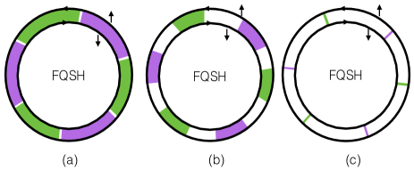
Figure 5: (a) A fractional quantum spin Hall edge in proximity to alternating ferromagnetic and superconducting strips. (b-c) By shrinking the size of the ferromagnetic and superconducting strips while at the same time increasing the strength of the proximity coupling, we can continuously deform the system into a fractional quantum spin Hall edge with magnetic and superconducting impurities.

III.5 Finite $U$ corrections

In the previous sections we analyzed the low energy physics of three different systems in the limit $U\rightarrow\infty$. In this section, we discuss how these results change when $U$ is large but finite.

III.5.1 Single magnetic impurity

We begin with the simplest case: a single magnetic impurity on the edge of a $\nu=1/k$ fractional quantum spin Hall state. We wish to understand how finite $U$ corrections affect the low energy spectrum derived in section III.2.

We follow the approach outlined in section II.4. According to this approach, the first step is to construct the operator $\Pi$ which is conjugate to the argument of the cosine term, $C=k(\phi_{\uparrow}(0)+\phi_{\downarrow}(0))$. To do this, we regularize $C$ as in equation (40), replacing $C\rightarrow\int_{-L/2}^{L/2}k(\phi_{\uparrow}(x)+\phi_{\downarrow}(x))\tilde{\delta}(x)dx$. For concreteness, we choose the regulated delta function $\tilde{\delta}$ to be

$$\tilde{\delta}(x)=\begin{cases}\frac{1}{b}&|x|\leq b/2\\ 0&|x|>b/2\end{cases}$$

With this regularization, we find:

$$[C,H_{0}] =\frac{kvi}{b}\int_{-b/2}^{b/2}{\color[rgb]{0,0,0}(\partial_{x}\phi_{\uparrow}-\partial_{x}\phi_{\downarrow})}dx$$

$$[C,[C,H_{0}]] =-\frac{4\pi kv}{b}$$

so that

$$\mathcal{M} =\frac{\pi b}{kv}$$

$$\Pi =\frac{1}{2}\int_{-b/2}^{b/2}{\color[rgb]{0,0,0}(\partial_{x}\phi_{\uparrow}-\partial_{x}\phi_{\downarrow})}dx$$

According to Eq. 23, the low energy theory at finite $U$ is obtained by adding terms to $H_{\text{eff}}$ (46) of the form $\sum_{n=-\infty}^{n=\infty}e^{in\Pi}\epsilon_{n}(\{a_{p},a_{p}^{\dagger}\},C_{3}^{\prime})$. Here, the $\epsilon_{n}$ are some unknown functions whose precise form cannot be determined without more calculation. We should mention that the $\epsilon_{n}$ functions also depend on $U$ — in fact, $\epsilon_{n}\rightarrow 0$ as $U\rightarrow\infty$ — but for notational simplicity we have chosen not to show this dependence explicitly. In what follows, instead of computing $\epsilon_{n}$, we take a more qualitative approach: we simply assume that $\epsilon_{n}$ contains all combinations of $a_{p},a_{p}^{\dagger},C_{3}^{\prime}$ that are not forbidden by locality or other general principles, and we derive the consequences of this assumption.

The next step is to analyze the effect of the above terms on the low energy spectrum. This analysis depends on which parameter regime one wishes to consider; here, we focus on the limit where $L\rightarrow\infty$, while $U$ is fixed but large. In this case, $H_{\text{eff}}$ (46) has a gapless spectrum, so we cannot use conventional perturbation theory to analyze the effect of the finite $U$ corrections; instead we need to use a renormalization group (RG) approach. This RG analysis has been carried out previously Kane and Fisher (1992a, b) and we will not repeat it here. Instead, we merely summarize a few key results: first, one of the terms generated by finite $U$, namely $e^{i\Pi}$, is relevant for $k>1$ and marginal for $k=1$. Second, the operator $e^{i\Pi}$ can be interpreted physically as describing a quasiparticle tunneling event where a charge $1/k$ quasiparticle tunnels from one side of the impurity to the other. Third, this operator drives the system from the $U=\infty$ fixed point to the $U=0$ fixed point.

These results imply that when $k>1$, for any finite $U$, the low energy spectrum in the thermodynamic limit $L\rightarrow\infty$ is always described by the $U=0$ theory $H_{0}$. Thus, in this case, the finite $U$ corrections have an important effect on the low energy physics. We note that these conclusions are consistent with the RG analysis of magnetic impurities given in Ref. Beri and Cooper, 2012.

III.5.2 Multiple magnetic impurities

We now move on to consider a system of $N$ equally spaced magnetic impurities on an edge of circumference $L$. As in the single impurity case, the first step in understanding the finite $U$ corrections is to compute the $\Pi_{i}$ operators that are conjugate to the $C_{i}$’s. Regularizing the cosine terms as in the previous case, a straightforward calculation gives

$$\mathcal{M}_{ij} =\frac{\pi b}{kv}\delta_{ij}$$

$$\Pi_{i} =\frac{1}{2}\int_{x_{i}-b/2}^{x_{i}+b/2}{\color[rgb]{0,0,0}(\partial_{x}\phi_{\uparrow}-\partial_{x}\phi_{\downarrow})}dx$$

where $i,j=1,...,N$.

According to Eq. 23, the finite $U$ corrections contribute additional terms to $H_{\text{eff}}$ (54) of the form $\sum_{\boldsymbol{n}}e^{i\sum_{j=1}^{N}n_{j}\Pi_{j}}\epsilon_{\boldsymbol{n}}$ where $\boldsymbol{n}=(n_{1},...,n_{N})$ is an $N$-component integer vector. Here, $\epsilon_{\boldsymbol{n}}$ is some unknown function of the operators $\{a_{pm},a_{pm}^{\dagger},C_{m}^{\prime}\}$ which vanishes as $U\rightarrow\infty$.

We now discuss how the addition of these terms affects the low energy spectrum in two different parameter regimes. First we consider the limit where $L\rightarrow\infty$ with $U$ and $N$ fixed. This case is a simple generalization of the single impurity system discussed above, and it is easy to see that the same renormalization group analysis applies here. Thus, in this limit the finite $U$ corrections have a dramatic effect for $k>1$ and cause the low energy spectrum to revert back to the $U=0$ system for any finite value of $U$, no matter how large.

The second parameter regime that we consider is where $L,N\rightarrow\infty$ with $U$ and $L/N$ fixed. The case is different from the previous one because $H_{\text{eff}}$ (54) has a finite energy gap in this limit (of order $v/s$ where $s=L/N$). Furthermore, $H_{\text{eff}}$ has a unique ground state. These two properties are stable to small perturbations, so we conclude that the system will continue to have a unique ground state and an energy gap for finite but sufficiently large $U$.

The presence of this energy gap at large $U$ is not surprising. Indeed, in the above limit, our system can be thought of as a toy model for a fractional quantum spin Hall edge that is proximity coupled to a ferromagnetic strip. It is well known that a ferromagnet can open up an energy gap at the edge if the coupling is sufficiently strongLevin and Stern (2009); Beri and Cooper (2012), which is exactly what we have found here.

III.5.3 Multiple magnetic and superconducting impurities

Finally, let us discuss a system of $2N$ equally spaced alternating magnetic and superconducting impurities on an edge of circumference $L$. As in the previous cases, the first step in understanding the finite $U$ corrections is to compute the $\Pi_{i}$ operators that are conjugate to the $C_{i}$’s. Regularizing the cosine terms as in the previous cases, a straightforward calculation gives

$$\mathcal{M}_{ij} = \frac{\pi b}{kv}\delta_{ij}$$

$$\Pi_{i} = \frac{1}{2}\int_{x_{i}-b/2}^{x_{i}+b/2}{\color[rgb]{0,0,0}(\partial_{x}\phi_{\uparrow}-(-1)^{i+1}\partial_{x}\phi_{\downarrow})}dx$$

where $i,j=1,...,2N$.

As a first step towards understanding the finite $U$ corrections, we consider a scenario in which only one of the impurities/cosine terms has a finite coupling constant $U$, while the others have a coupling constant which is infinitely large. This scenario is easy to analyze because we only have to include the corrections associated with a single impurity. For concreteness, we assume that the impurity in question is superconducting rather than magnetic and we label the corresponding cosine term by $\cos(C_{2j})$ (in our notation the superconducting impurities are labeled by even integers). Having made these choices, we can immediately write down the finite $U$ corrections: according to Eq. 23, these corrections take the form

$${\color[rgb]{0,0,0}\sum_{n=-\infty}^{\infty}}e^{in\Pi_{2j}}\epsilon_{n}(\{a_{pm},a_{pm}^{\dagger}\}),$$

where the $\epsilon_{n}$ are some unknown functions which vanish as $U\rightarrow\infty$.

Our next task is to understand how these corrections affect the low energy spectrum. The answer to this question depends on which parameter regime one wishes to study: here we will focus on the regime where $L,N\rightarrow\infty$ with $L/N$ and $U$ fixed. In this limit, $H_{\text{eff}}$ (65) has a finite energy gap of order $v/s$ where $s=L/N$. At the same time, the ground state is highly degenerate: in fact, the degeneracy is exponentially large in the system size, growing as $D=2\cdot(2k)^{N-2}$. Given this energy spectrum, it follows that at the lowest energy scales, the only effect of the finite $U$ corrections is to split the ground state degeneracy.

To analyze this splitting, we need to compute the matrix elements of the finite $U$ corrections between different ground states and then diagonalize the resulting $D\times D$ matrix. Our strategy will be to use the identity (26) which relates the matrix elements of the finite $U$ corrections to the matrix elements of $e^{ni\Gamma_{2j}}$. Following this approach, the first step in our calculation is to compute $\Gamma_{2j}$. Using the definition (24), we find

$$\Gamma_{2j}=\frac{1}{2k}(C_{2j+1}-C_{2j-1})$$

assuming $j\neq N$. (The case $j=N$ is slightly more complicated due to our conventions for describing the periodic boundary conditions at the edge, so we will assume $j\neq N$ in what follows).

The next step is to find the matrix elements of the operator $e^{in\Gamma_{2j}}$ between different ground states. To this end, we rewrite $\Gamma_{2j}$ in terms of the $C_{i}^{\prime}$ operators: $\Gamma_{2j}=\frac{C_{j}^{\prime}}{2k}$. The matrix elements of $e^{in\Gamma_{2j}}$ can now be computed straightforwardly using the known matrix elements of $C_{j}^{\prime}$ (see Eqs. 149-150):

$$\langle\boldsymbol{\alpha}^{\prime}|e^{in\Gamma_{2j}}|\boldsymbol{\alpha}\rangle=e^{\frac{\pi in\alpha_{j}}{k}}\delta_{\boldsymbol{\alpha}^{\prime}\boldsymbol{\alpha}}$$ (69)

where $|\boldsymbol{\alpha}\rangle$ denotes the ground state $|\boldsymbol{\alpha}\rangle\equiv|\boldsymbol{\alpha},\boldsymbol{n}=0\rangle$.

At this point we apply the identity (26) which states that the matrix elements of $e^{in\Pi_{2j}}\epsilon_{n}(\{a_{pm},a_{pm}^{\dagger}\})$ are equal to the matrix elements of $u_{n}\cdot e^{in\Gamma_{2j}}$ where $u_{n}$ is some unknown proportionality constant. Using this identity together with (69), we conclude that the matrix elements of the finite $U$ corrections are given by

$$f\left(\frac{\alpha_{j}}{k}\right)\delta_{\boldsymbol{\alpha}^{\prime}\boldsymbol{\alpha}}$$

where $f(x)=\sum_{n=-\infty}^{\infty}u_{n}e^{\pi inx}$.

We are now in position to determine the splitting of the ground states. To do this, we note that while we don’t know the values of the $u_{n}$ constants and therefore we don’t know $f(x)$, we expect that generically the function $f$ will have a unique minimum for $\alpha_{j}\in\{0,1,...,2k-1\}$. Assuming this is the case, we conclude that the finite $U$ corrections favor a particular value of $\alpha_{j}$, say $\alpha_{j}=0$. Thus these corrections reduce the ground state degeneracy from $D$ to $D/2k$.

So far we have analyzed the case where one of the superconducting impurities is characterized by a finite coupling constant $U$ while the other impurities are at infinite coupling. Next, suppose that all the superconducting impurities have finite $U$ while all the magnetic impurities have infinite $U$. In this case, similar analysis as above shows that the matrix elements of the finite $U$ corrections are of the following form:

$$\left[\sum_{j=1}^{N-1}f\left(\frac{\alpha_{j}}{k}\right)+f\left(\alpha_{N}-\frac{1}{k}\sum_{j=1}^{N-1}\alpha_{j}\right)\right]\delta_{\boldsymbol{\alpha}^{\prime}\boldsymbol{\alpha}}$$ (70)

To determine the splitting of the ground states, we need to understand the eigenvalue spectrum of the above matrix. Let us assume that $f$ has a unique minimum at some $\alpha_{j}=q$ — which is what we expect generically. Then, as long as the system size is commensurate with this value in the sense that $Nq$ is a multiple of $k$, we can see that the above matrix has a unique ground state $|\boldsymbol{\alpha}\rangle$ with $\alpha_{1}=...=\alpha_{N-1}=q$ and $\alpha_{N}=Nq/k$ (mod $2$). Furthermore, this ground state is separated from the lowest excited states by a finite gap, which is set by the function $f$. Thus, in this case, the finite $U$ corrections completely split the ground state degeneracy leading to a unique ground state with an energy gap.

Likewise, we can consider the opposite scenario where the magnetic impurities have finite $U$ while the superconducting impurities have infinite $U$. Again, similar analysis shows that the corrections favor a unique ground state which is separated from the excited states by a finite gap. The main difference from the previous case is that the matrix elements of the finite $U$ corrections are off-diagonal in the $|\boldsymbol{\alpha}\rangle$ basis so the ground state is a superposition of many different $|\boldsymbol{\alpha}\rangle$ states.

To complete the discussion, let us consider the case where all the impurities, magnetic and superconducting, have finite $U$. If the magnetic impurities are at much stronger coupling than the superconducting impurities or vice-versa then presumably the finite $U$ corrections drive the system to one of the two gapped phases discussed above. On the other hand, if the two types of impurities have comparable values of $U$, then the low energy physics is more delicate since the finite $U$ corrections associated with the two types of impurities do not commute with one other, i.e. $[e^{i\Gamma_{2j}},e^{i\Gamma_{2j\pm 1}}]\neq 0$. In this case, a more quantitative analysis is required to determine the fate of the low energy spectrum.

IV Conclusion

In this paper we have presented a general recipe for computing the low energy spectrum of Hamiltonians of the form (1) in the limit $U\rightarrow\infty$. This recipe is based on the construction of an effective Hamiltonian $H_{\text{eff}}$ and an effective Hilbert space $\mathcal{H}_{\text{eff}}$ describing the low energy properties of our system in the infinite $U$ limit. The key reason that our approach works is that this effective Hamiltonian is quadratic, so there is a simple procedure for diagonalizing it.

While our recipe gives exact results in the infinite $U$ limit, it provides only approximate results when $U$ is finite; in order to obtain the exact spectrum in the finite $U$ case, we need to include additional (non-quadratic) terms in $H_{\text{eff}}$. As part of this work, we have discussed the general form of these finite $U$ corrections and how they scale with $U$. However, we have not discussed how to actually compute these corrections. One direction for future research would be to develop quantitative approaches for obtaining these corrections — for example using the instanton approach outlined in Ref. Coleman, 1988.

Some of the most promising directions for future work involve applications of our formalism to different physical systems. In this paper, we have focused on the application to Abelian fractional quantum Hall edges, but there are several other systems where our formalism could be useful. For example, it would be interesting to apply our methods to superconducting circuits — quantum circuits built out of inductors, capacitors, and Josephson junctions. In particular, several authors have identified superconducting circuits with protected ground state degeneracies that could be used as qubits.Kitaev ; Gladchenko et al. (2009); Brooks et al. (2013); Dempster et al. (2014) The formalism developed here might be useful for finding other circuits with protected degeneracies.

Appendix A Derivation of low energy effective theory

In this appendix, we derive an effective theory that describes the low energy spectrum of $H$ (1) in the limit $U\rightarrow\infty$. More specifically, we show that the low energy spectrum of $H$ in the infinite $U$ limit is described by the effective Hamiltonian $H_{\text{eff}}$ (2), which is defined within the effective Hilbert space $\mathcal{H}_{\text{eff}}$ (5). Before proving this result in generality, we first derive it for two illustrative examples in appendix A.1 and a special case in appendix A.2. Finally, after this preparation, we work out the general case in appendix A.3.

A.1 Two examples

A.1.1 Harmonic oscillator with a cosine term

To understand the basic ideas underlying the derivation, it is helpful to consider some simple examples. We start by studying a one dimensional harmonic oscillator with a cosine term:

$$H=\frac{p^{2}}{2m}+\frac{Kx^{2}}{2}-U\cos(2\pi x)$$ (71)

In the following, we derive an effective Hamiltonian $H_{\text{eff}}$ and effective Hilbert space $\mathcal{H}_{\text{eff}}$ that describe the low energy spectrum of $H$ in the limit $U\rightarrow\infty$.

To begin, we decompose $H$ into two pieces, $H=H_{1}+H_{2}$, where

$$H_{1}=\frac{p^{2}}{2m}-U\cos(2\pi x),\quad\quad H_{2}=\frac{Kx^{2}}{2}$$ (72)

Our strategy is as follows: first, we show that when $U$ is large, $H_{1}$ has a collection of nearly degenerate ground states which are separated from the lowest excited states by a large gap. Next we argue that we can treat $H_{2}$ as a perturbation which splits the ground state degeneracy of $H_{1}$. Finally, using degenerate perturbation theory, we derive a low energy effective Hamiltonian for our system.

Following this plan, we start with the Hamiltonian $H_{1}$. This Hamiltonian describes a one dimensional particle moving in a cosine potential. The low energy physics of $H_{1}$ is especially simple when $U$ is large. In this case, tunneling between the different cosine minima is suppressed so that $H_{1}$ has an infinite set of nearly degenerate ground states — one for each cosine minimum. We will label these states as $\{|\psi_{q}\rangle\}$ where $|\psi_{q}\rangle$ is localized around the minimum $x=q$ and $q=0,\pm 1,\pm 2,...$.

We can estimate the energy gap of $H_{1}$ by expanding the cosine potential to quadratic order in $x$: $U\cos(2\pi x)\approx U(1-2\pi^{2}x^{2})$. In this approximation, the cosine potential is equivalent to a harmonic oscillator with frequency $\omega=2\pi\sqrt{U/m}$. In particular, it follows that the ground states of $H_{1}$ are separated from the lowest excited states by an energy gap $\Delta$ of order $\Delta\sim\sqrt{U/m}$.

Now let us imagine adding $H_{2}$ to $H_{1}$. We would like to know how $H_{2}$ splits the degeneracy between the ground states $|\psi_{q}\rangle$. To answer this question, we will treat $H_{2}$ as a perturbation to $H_{1}$ and then we will compute the associated energy splitting using degenerate perturbation theory. However, before we do this, we first need to check that such a perturbative approach is justified in the infinite $U$ limit. To this end, we need to estimate the size of the matrix element $\langle\psi_{ex}|H_{2}|\psi_{q}\rangle$ where $|\psi_{q}\rangle$ is an arbitrary ground state and $|\psi_{ex}\rangle$ is an arbitrary excited state of $H_{1}$. For large $U$ we can approximate $|\psi_{q}\rangle$ by a harmonic oscillator ground state centered at position $x=q$. Similarly, we can approximate $|\psi_{ex}\rangle$ by the $n$th excited state of the harmonic oscillator centered at $x=q$. Within this approximation, the matrix element $\langle\psi_{ex}|H_{2}|\psi_{q}\rangle$ reduces to

$$\langle\psi_{ex}|H_{2}|\psi_{q}\rangle\approx\langle n|K(x+q)^{2}|0\rangle$$ (73)

where $|0\rangle$ and $|n\rangle$ are the ground state and $n$th excited state of a harmonic oscillator with frequency $\omega=2\pi\sqrt{U/m}$, centered at $x=0$. The latter matrix element can be evaluated easily with the result

$$\langle n|K(x+q)^{2}|0\rangle\sim\begin{cases}\frac{Kq}{(mU)^{1/4}}&\mbox{if }n=1\\ \frac{K}{\sqrt{mU}}&\mbox{if }n=2\\ 0&\mbox{if }n\geq 3\end{cases}$$

Combining this expression with our formula for the energy gap $\Delta$, we obtain

$$\sum_{|\psi_{ex}\rangle}\frac{|\langle\psi_{ex}|H_{2}|\psi_{q}\rangle|^{2}}{\Delta}\sim\frac{K^{2}q^{2}}{U}$$ (74)

in the large $U$ limit. This estimate is significant because the left hand side of (74) is proportional to the second order perturbative correction to the ground state energies. Evidently, this correction vanishes as $U\rightarrow\infty$, so we conclude that first order perturbation theory gives exact results in this limit.

With this justification, we now proceed with the perturbative calculation. According to first order degenerate perturbation theory, the energy splitting of the ground states can be determined by diagonalizing the matrix $\langle\psi_{q^{\prime}}|H_{2}|\psi_{q}\rangle$. When $U$ is large, $|\psi_{q}\rangle$ can be approximated as a Gaussian wave function, centered at $x=q$. The width of this Gaussian is given by:

$$(\Delta x)^{2}\sim\frac{1}{m\omega}\sim\frac{1}{\sqrt{mU}}$$

We see that as $U\rightarrow\infty$, $(\Delta x)^{2}\rightarrow 0$ so that $|\psi_{q}\rangle$ approaches a position eigenstate: $|\psi_{q}\rangle\rightarrow|x=q\rangle$. We conclude that the low energy spectrum of $H$ can be obtained by diagonalizing the matrix $\langle q^{\prime}|H_{2}|q\rangle$.

At this point, our calculation is essentially complete: the matrix elements $\langle q^{\prime}|H_{2}|q\rangle$ define our low energy effective Hamiltonian, while the ground state subspace spanned by $\{|q\rangle\}$ defines our low energy Hilbert space. In other words, the low energy effective Hamiltonian is given by

$$H_{\text{eff}}=H_{2}=\frac{Kx^{2}}{2}$$ (75)

while the low energy effective Hilbert space $\mathcal{H}_{\text{eff}}$ is the subspace spanned by position eigenstates $\{|q\rangle\}$ for $q=0,\pm 1,\pm 2...$. Clearly this effective theory is valid for energies smaller than the gap of $H_{1}$, i.e. $E<2\pi\sqrt{U/m}$.

Comparing these expressions with the effective Hamiltonian and Hilbert space from section II.1, we see that they agree exactly. Thus we have successfully established equations (2) and (5) for this example.

A.1.2 Harmonic oscillator with 2 cosine terms

Another important illustrative example is given by a one dimensional harmonic oscillator with two cosine terms:

$$H=\frac{p^{2}}{2m}+\frac{Kx^{2}}{2}-U\cos(dp)-U\cos(2\pi x)$$ (76)

Here, $d$ is a positive integer.

Before analyzing $H$ we need to choose an appropriate basis in which to represent it. Because the arguments of the two cosine terms don’t commute with one another, neither the position basis nor the momentum basis are particularly convenient choices. Instead, we find it helpful to work in a third basis, which consists of simultaneous eigenstates of the commuting operators $e^{ip},e^{2\pi ix}$. We will denote these simultaneous eigenstates by $|\theta,\varphi\rangle$ where

$$e^{ip}|\theta,\varphi\rangle =e^{i\theta}|\theta,\varphi\rangle$$

$$e^{2\pi ix}|\theta,\varphi\rangle =e^{i\varphi}|\theta,\varphi\rangle$$ (77)

Here, the labels $\theta,\varphi$ take values in $0\leq\theta,\varphi<2\pi$. The explicit formula for $|\theta,\varphi\rangle$ is

$$|\theta,\varphi\rangle=\frac{1}{\sqrt{2\pi}}\sum_{j}e^{ij\theta}|j+\frac{\varphi}{2\pi}\rangle$$ (78)

where $|j+\frac{\varphi}{2\pi}\rangle$ denotes the position eigenstate at position $x=j+\frac{\varphi}{2\pi}$.

We now work out what the Hamiltonian $H$ looks like in the $\theta,\varphi$ representation. The first step is to express the $x,p$ operators in terms of $\theta,\varphi$. To this end, we observe that

$$e^{iax}|\theta,\varphi\rangle = e^{ia\varphi/2\pi}|\theta+a,\varphi\rangle$$

$$e^{iap}|\theta,\varphi\rangle = |\theta,\varphi-2\pi a\rangle$$

Differentiating these equations with respect to $a$, we derive

$$x|\theta,\varphi\rangle = \left(\frac{1}{i}\frac{\partial}{\partial\theta}+\frac{\varphi}{2\pi}\right)|\theta,\varphi\rangle$$

$$p|\theta,\varphi\rangle = -\frac{2\pi}{i}\frac{\partial}{\partial\varphi}|\theta,\varphi\rangle$$

From these equations, we deduce that

$$\langle\theta,\varphi|x|\psi\rangle = \left(-\frac{1}{i}\frac{\partial}{\partial\theta}+\frac{\varphi}{2\pi}\right)\langle\theta,\varphi|\psi\rangle$$

$$\langle\theta,\varphi|p|\psi\rangle = \frac{2\pi}{i}\frac{\partial}{\partial\varphi}\langle\theta,\varphi|\psi\rangle$$

for any state $|\psi\rangle$. We conclude that in the $\theta,\varphi$ representation, the operators $x,p$ take the form

$$x=-\frac{1}{i}\frac{\partial}{\partial\theta}+\frac{\varphi}{2\pi},\quad p=\frac{2\pi}{i}\frac{\partial}{\partial\varphi}$$

or equivalently

$$x=-p_{\theta}+\frac{\varphi}{2\pi},\quad p=2\pi p_{\varphi}$$ (79)

where $p_{\theta}\equiv\frac{1}{i}\frac{\partial}{\partial\theta}$ and $p_{\varphi}\equiv\frac{1}{i}\frac{\partial}{\partial\varphi}$.

The next step is to find expressions for $e^{2\pi ix}$ and $e^{ip}$ in terms of $\theta,\varphi$. One way to do this is to exponentiate (79):

$$e^{2\pi ix}=e^{-2\pi ip_{\theta}+i\varphi},\quad e^{ip}=e^{2\pi ip_{\varphi}}$$

We then make use of two operator identities which we will prove shortly:

$$e^{2\pi ip_{\theta}}=1,\quad e^{2\pi ip_{\varphi}}=e^{i\theta}$$ (80)

With these identities, we can simplify the expressions for $e^{2\pi ix}$ and $e^{ip}$ to:

$$e^{2\pi ix}=e^{i\varphi},\quad e^{ip}=e^{i\theta}$$ (81)

(Alternatively, we could also have derived (81) directly from (77)). The proof of the identities (80) relies on the following observations:

$$e^{2\pi ip_{\theta}}|\theta,\varphi\rangle=|\theta-2\pi,\varphi\rangle,\quad e^{2\pi ip_{\varphi}}|\theta,\varphi\rangle=|\theta,\varphi-2\pi\rangle$$

and

$$|\theta-2\pi,\varphi\rangle=|\theta,\varphi\rangle,\quad|\theta,\varphi-2\pi\rangle=e^{i\theta}|\theta,\varphi\rangle$$

Putting these together, we deduce that

$$e^{2\pi ip_{\theta}}|\theta,\varphi\rangle=|\theta,\varphi\rangle,\quad e^{2\pi ip_{\varphi}}|\theta,\varphi\rangle=e^{i\theta}|\theta,\varphi\rangle$$

Since these relations hold for all basis states, they imply the operator identities (80).

We now have all the ingredients to write the Hamiltonian $H$ in terms of $\theta,\varphi$: combining (79) and (81), we derive

$$H = \frac{4\pi^{2}p_{\varphi}^{2}}{2m}+\frac{K(p_{\theta}-\varphi/2\pi)^{2}}{2}$$ (82)

$$- U\cos(d\theta)-U\cos(\varphi)$$

This Hamiltonian is defined on a Hilbert space consisting of wave functions $\psi(\theta,\varphi)$ with $0\leq\theta,\varphi<2\pi$. To find the boundary conditions for these wave functions, we use the identities

$$|\theta,2\pi\rangle=e^{-i\theta}|\theta,0\rangle,\quad|2\pi,\varphi\rangle=|0,\varphi\rangle$$

which follow from the definition of $|\theta,\varphi\rangle$. These identities imply that our wave functions $\psi$ satisfy the boundary conditions

$$\psi(\theta,2\pi)=e^{i\theta}\psi(\theta,0),\quad\psi(2\pi,\varphi)=\psi(0,\varphi)$$ (83)

So far, all we have done is derive the $\theta,\varphi$ representation (82) of the Hamiltonian and the Hilbert space (83). We now use this representation to find the low energy spectrum of $H$ in the large $U$ limit. To begin, we note that $H$ can be thought of as describing a particle on a torus parameterized by $\theta,\varphi$. This particle is coupled to a vector potential and two cosine potentials. Now consider the limit where $U$ is large. In this limit, tunneling between the different cosine minima is suppressed, so we conclude that $H$ has a set of nearly degenerate ground states, each of which is localized in a different minimum. There are $d$ different cosine minima located at positions $(\theta,\varphi)=(2\pi\alpha/d,0)$, with $\alpha=0,1,...,d-1$, so $H$ has $d$ ground states. We will label these states by $|\psi_{\alpha}\rangle$.

To estimate the energy gap separating the ground states from the lowest excited states, we expand the cosine potentials to quadratic order. In this approximation, $H$ reduces to a sum of two decoupled harmonic oscillators with frequencies $\sqrt{U/m}$ and $\sqrt{UK}$. We conclude that the energy gap is of order $\Delta\sim\text{min}(\sqrt{U/m},\sqrt{UK})$.

Let us now translate these results into the language of effective Hamiltonians. We have seen that $H$ has $d$ ground states $|\psi_{\alpha}\rangle$. We have also seen that these states are separated from the excited states by a large gap $\Delta$. Furthermore, it is easy to see that when $U\rightarrow\infty$, the width of $|\psi_{\alpha}\rangle$ becomes vanishingly small, so that $|\psi_{\alpha}\rangle$ approaches the state $|\theta=\frac{2\pi\alpha}{d},\varphi=0\rangle$:

$$|\psi_{\alpha}\rangle\rightarrow|\theta=\frac{2\pi\alpha}{d},\varphi=0\rangle$$

Putting this all together, we conclude that the low energy spectrum of $H$ is described by an effective Hamiltonian, $H_{\text{eff}}=0$ defined within an effective $d$-dimensional Hilbert space $\mathcal{H}_{\text{eff}}$ spanned by the states $|\theta=\frac{2\pi\alpha}{d},\varphi=0\rangle$, with $\alpha=0,1,...,d-1$. This effective description is valid for energies $E<\Delta$. (Here, the reason we use $H_{\text{eff}}=0$ rather than $H_{\text{eff}}=\text{const.}$ is that we only interested in energy differences and therefore we are free to redefine the ground state energy to be $0$). Comparing these results with the effective Hamiltonian and Hilbert space from section II.1, we can see that there is exact agreement.

A.2 Special case

We now generalize the example of appendix A.1.1 to a Hamiltonian of the form

$$H=H_{0}-U\sum_{i=1}^{M}\cos(2\pi x_{i}),$$ (84)

defined on the $2N$ dimensional phase space $\{x_{1},...,x_{N},p_{1},...,p_{N}\}$ with $[x_{i},p_{j}]=i\delta_{ij}$. Here $H_{0}$ is an arbitrary positive semidefinite quadratic function of $\{x_{1},...,x_{N},p_{1},...,p_{N}\}$ with the only restriction being that the $M\times M$ matrix

$$\mathcal{N}_{ij}=-[x_{i},[x_{j},H_{0}]]$$ (85)

is non-degenerate.

Following the same outline as in the previous sections, we first derive an effective Hamiltonian and effective Hilbert space that describe the low energy spectrum of $H$ in the infinite $U$ limit, and then we show that this effective theory agrees with the general expressions from equations (2) and (5).

For the first step, we use the same strategy as in appendix A.1.1: we decompose the Hamiltonian into two pieces, $H=H_{1}+H_{2}$, where

$$H_{1} =\sum_{i,j=1}^{M}\frac{(\mathcal{M}^{-1})_{ij}}{2}\cdot\Pi_{i}\Pi_{j}-U\sum_{i=1}^{M}\cos(2\pi x_{i})$$

$$H_{2} =H_{0}-\sum_{i,j=1}^{M}\frac{(\mathcal{M}^{-1})_{ij}}{2}\cdot\Pi_{i}\Pi_{j}$$ (86)

Here $\mathcal{M}_{ij}$ is an $M\times M$ scalar matrix defined by $\mathcal{M}=\mathcal{N}^{-1}$ and $\Pi_{1},...,\Pi_{M}$ are operators defined by

$$\Pi_{i}=-i\sum_{j=1}^{M}\mathcal{M}_{ij}[x_{j},H_{0}]$$ (87)

After making this decomposition, we will treat $H_{2}$ as a perturbation to $H_{1}$ and then derive an effective Hamiltonian using first order degenerate perturbation theory.

Before executing this plan, we first make some preliminary observations. One observation is that

$$[x_{i},\Pi_{j}]=i\delta_{ij},\quad i=1,...,M$$ (88)

Another observation is that we can assume without loss of generality that

$$[x_{i},\Pi_{j}]=[p_{i},\Pi_{j}]=0,\quad i=M+1,...,N$$ (89)

The reason why we can assume (89) is that we can always redefine the position and momentum operators $x_{i},p_{i}$ for $i=M+1,...,N$ according to

$$x_{i}\rightarrow x_{i}+\sum_{k=1}^{M}a_{ik}x_{k},\quad p_{i}\rightarrow p_{i}+\sum_{k=1}^{M}b_{ik}x_{k}$$

where $a_{ik}=i[x_{i},\Pi_{k}]$ and $b_{ik}=i[p_{i},\Pi_{k}]$. After this redefinition, Eq. 89 is automatically satisfied. A final observation is that $\Pi_{j}$ can be written in the form

$$\Pi_{j}=p_{j}+A_{j}$$ (90)

where $A_{j}$ is a linear combination of $\{x_{1},...,x_{M}\}$. Indeed, this result follows immediately from (88) and (89).

With these observations in mind, we now study the low energy spectrum of $H_{1}$. To begin we note that (90) implies that $H_{1}$ can be written in the form

$$H_{1}=\sum_{i,j=1}^{M}\frac{(\mathcal{M}^{-1})_{ij}}{2}\cdot(p_{i}+A_{i})(p_{j}+A_{j})-U\sum_{i=1}^{M}\cos(2\pi x_{i})$$

where $A_{j}$ is a linear function of $\{x_{1},...,x_{M}\}$. Next, we note that $[x_{i},H_{1}]=0$ for $i=M+1,...,N$, which implies that $H_{1}$ can be diagonalized separately for each value of $\boldsymbol{x}_{\perp}=(x_{M+1},...,x_{N})$. Once we fix $\boldsymbol{x}_{\perp}$, the Hamiltonian $H_{1}$ describes an $M$ dimensional particle with coordinates $(x_{1},...,x_{M})$, moving in a periodic potential $-U\sum_{i=1}^{M}\cos(x_{i})$ and coupled to a vector potential $A$ that depends linearly on $\{x_{1},...,x_{M}\}$. Let us consider the low energy physics of this $M$ dimensional particle when $U$ is large. In this case, we can neglect tunneling between the different minima of the cosine potential, and treat each minimum in isolation. At the same time, it is easy to see that the energy spectra associated with different cosine minima and different values of $\boldsymbol{x}_{\perp}$ are all identical since $H_{1}$ has discrete (magnetic) translational invariance in the $x_{1},...,x_{M}$ directions as well as continuous translational invariance in the $x_{M+1},...,x_{N}$ directions. Putting these facts together, we conclude that the Hamiltonian $H_{1}$ has an infinite set of nearly degenerate ground states — one ground state for each cosine minimum and each value of $\boldsymbol{x}_{\perp}$. We label these ground states as $|\psi_{\boldsymbol{q},\boldsymbol{x}_{\perp}}\rangle$ where $\boldsymbol{q}=(q_{1},...,q_{M})$ is an $M$ component integer vector describing the position of the cosine minimum and $\boldsymbol{x}_{\perp}=(x_{M+1},...,x_{N})$ is an $N-M$ component real vector describing the position in the orthogonal directions.

We can estimate the energy gap between the ground states and excited states of $H_{1}$ by expanding the cosine potential to quadratic order in $\boldsymbol{x}$. In this approximation, the cosine potential reduces to a multidimensional quadratic potential. Diagonalizing this potential gives a collection of harmonic oscillators with frequencies $\omega_{i}=\sqrt{U/m_{i}}$ where $m_{i}$ are the eigenvalues of the matrix $\mathcal{M}_{ij}$. The energy gap is determined by the smallest frequency and thus the largest eigenvalue $m_{i}$. We conclude that $H_{1}$ has an energy gap $\Delta\sim\sqrt{U/m}$ where $m$ is the maximum eigenvalue of $\mathcal{M}_{ij}$.

We now imagine adding $H_{2}$ to $H_{1}$, and we ask how the low energy spectrum changes. As in appendix A.1.1, we will answer this question using a perturbative expansion in $H_{2}$. However, before we perform this calculation, we need to check that this perturbative approach is valid when $U$ is large. To this end, we need to estimate the size of the matrix elements $\langle\psi_{ex}|H_{2}|\psi_{\boldsymbol{q},\boldsymbol{x}_{\perp}}\rangle$ where $|\psi_{\boldsymbol{q},\boldsymbol{x}_{\perp}}\rangle$, $|\psi_{ex}\rangle$ are arbitrary ground states and excited states of $H_{1}$. The first step is to observe that $H_{2}$ has a special property: for any $i=1,...,M$, we have

$$[x_{i},H_{2}] = [x_{i},H_{0}]-i\sum_{j=1}^{M}(\mathcal{M}^{-1})_{ij}\cdot\Pi_{j}$$

$$= [x_{i},H_{0}]-[x_{i},H_{0}]$$

$$= 0$$

It follows that the momentum operators $p_{1},...,p_{M}$ do not appear in $H_{2}$. Thus, $H_{2}$ is a sum of three types of terms: $x_{i}x_{j}$, $p_{k}p_{l}$ and $x_{i}p_{k}$, where $i,j$ are arbitrary and $k,l\geq M+1$. We need to estimate the matrix elements corresponding to each of these terms. We can do this using the same argument as in appendix A.1.1. First, we note that when $U$ is large, the states $|\psi_{\boldsymbol{q},\boldsymbol{x}_{\perp}}\rangle$ and $|\psi_{ex}\rangle$ can be approximated as harmonic oscillator eigenstates centered at some appropriate positions in space. The matrix elements of interest can then be related to harmonic oscillator matrix elements as in Eq. 73. Omitting details, a straightforward calculation shows that all three types of matrix elements fall off like $U^{-1/4}$ or faster as $U\rightarrow\infty$. Combining this scaling law with the expression for $\Delta$, we see that

$$\sum_{|\psi_{ex}\rangle}\frac{|\langle\psi_{ex}|H_{2}|\psi_{q}\rangle|^{2}}{\Delta}=O\left(\frac{1}{U}\right)$$

As in appendix A.1.1, this estimate implies that the second order perturbative corrections to the ground state energies vanish in the limit $U\rightarrow\infty$. Therefore, first order perturbation theory is exact in this limit.

We now proceed with the perturbative calculation. According to first order degenerate perturbation theory, the energy splitting of the ground states can be determined by diagonalizing the matrix $\langle\psi_{\boldsymbol{q}^{\prime},\boldsymbol{x}^{\prime}_{\perp}}|H_{2}|\psi_{\boldsymbol{q},\boldsymbol{x}_{\perp}}\rangle$. These matrix elements are easy to compute. Indeed, for large $U$, the ground states $|\psi_{\boldsymbol{q},\boldsymbol{x}_{\perp}}\rangle$ can be approximated as harmonic oscillator ground states with a width of order $(\Delta x)^{2}\sim\frac{1}{\sqrt{mU}}$. In the limit $U\rightarrow\infty$, the width $\Delta x\rightarrow 0$ so $|\psi_{\boldsymbol{q},\boldsymbol{x}_{\perp}}\rangle$ approaches a position eigenstate: $|\psi_{\boldsymbol{q},\boldsymbol{x}_{\perp}}\rangle\rightarrow|\boldsymbol{q},\boldsymbol{x}_{\perp}\rangle$ where $|\boldsymbol{q},\boldsymbol{x}_{\perp}\rangle$ denotes the position eigenstate located at $\boldsymbol{x}=(\boldsymbol{q},\boldsymbol{x}_{\perp})$. Thus, in this limit, the matrix we need to diagonalize is $\langle\boldsymbol{q}^{\prime},\boldsymbol{x}^{\prime}_{\perp}|H_{2}|\boldsymbol{q},\boldsymbol{x}_{\perp}\rangle$.

Our calculation is now complete: we have shown that the low energy spectrum of $H$ in the limit $U\rightarrow\infty$ can be obtained by diagonalizing the operator $H_{2}$ within the subspace spanned by $\{|\boldsymbol{q},\boldsymbol{x}_{\perp}\rangle\}$. In other words, the effective Hamiltonian for our system is

$$H_{\text{eff}} = H_{2}$$ (91)

$$= H_{0}-\sum_{i,j=1}^{M}\frac{(\mathcal{M}^{-1})_{ij}}{2}\cdot\Pi_{i}\Pi_{j}$$

while the effective Hilbert space $\mathcal{H}_{\text{eff}}$ is spanned by position eigenstates $\{|\boldsymbol{q},\boldsymbol{x}_{\perp}\rangle\}$ for which the first $M$ components $q_{1},...,q_{M}$ are integers and the last $N-M$ components $x_{M+1},...,x_{N}$ are real valued. This effective theory is valid for energies $E\lesssim\sqrt{U/m}$.

Comparing the above effective Hamiltonian and Hilbert space with the general expressions from equations (2) and (5), we can see that they match exactly. This completes our proof of equations (2), (5) for the special case (84).

A.3 General case

To complete the derivation of equations (2) and (5), we now consider the most general case:

$$H=H_{0}-U\sum_{i=1}^{M}\cos(C_{i}),\ \ C_{i}=\sum_{j=1}^{N}(\gamma_{ij}x_{j}+\gamma_{ij}^{\prime}p_{j}+\delta_{i})$$ (92)

Here $H$ is defined on a $2N$ dimensional phase space $\{x_{1},...,x_{N},p_{1},...,p_{N}\}$ with $[x_{i},p_{j}]=i\delta_{ij}$. The first term $H_{0}$ is a positive semidefinite quadratic function of $\{x_{1},...,x_{N},p_{1},...,p_{N}\}$ and $\gamma_{ij},\gamma_{ij}^{\prime},\delta_{i}$ are arbitrary real numbers with the only constraints being that (1) $\{C_{1},...,C_{M}\}$ are linearly independent, (2) $[C_{i},C_{j}]$ is an integer multiple of $2\pi i$ for all $i,j$ so that the different cosine terms commute with one another, and (3) the matrix

$$\mathcal{N}_{ij}=-\frac{1}{4\pi^{2}}[C_{i},[C_{j},H_{0}]]$$ (93)

is non-degenerate. Our task is to derive an effective Hamiltonian and effective Hilbert space that describes the low energy spectrum of $H$ in the limit $U\rightarrow\infty$. We will then show that this effective theory is exactly the one defined in equations (2) and (5).

Our basic strategy is simple: we will map $H$ onto the Hamiltonian studied in the previous section and then we will derive the effective theory using our previous results. While this is a simple plan at a conceptual level, there are some technical obstacles that make it difficult to define the desired mapping in one step. Therefore, we will build up the mapping in stages by making several successive changes of variables.

In the first change of variables, we replace $x_{i},p_{i}$ by new coordinates $x_{i}^{\prime},p_{i}^{\prime}$ which are chosen so that the constraints $C_{i}$ can be written as integer linear combinations of $2\pi x_{i}^{\prime}$ and $p_{i}^{\prime}$. To this end, it is helpful to consider the $M\times M$ matrix $\mathcal{Z}_{ij}$ defined by

$$\mathcal{Z}_{ij}=\frac{1}{2\pi i}[C_{i},C_{j}]$$ (94)

Clearly the matrix $\mathcal{Z}_{ij}$ is integer and skew-symmetric. Therefore, there exists an integer matrix $\mathcal{V}$ with determinant $\pm 1$ such that $\mathcal{V}\mathcal{Z}\mathcal{V}^{T}=\mathcal{Z}^{\prime}$ where $\mathcal{Z}^{\prime}$ is in skew-normal formNewman (1972):

$$\mathcal{Z}^{\prime}=\begin{pmatrix}0_{I}&-\mathcal{D}&0\\ \mathcal{D}&0_{I}&0\\ 0&0&0_{M-2I}\end{pmatrix},\ \ \mathcal{D}=\begin{pmatrix}d_{1}&0&\dots&0\\ 0&d_{2}&\dots&0\\ \vdots&\vdots&\vdots&\vdots\\ 0&0&\dots&d_{I}\end{pmatrix}$$ (95)

Here $0\leq I\leq M/2$ and $0_{I}$ denotes an $I\times I$ matrix of zeros, and similarly for $0_{M-2I}$. Let

$$C_{i}^{\prime}=\sum_{j=1}^{M}\mathcal{V}_{ij}C_{j}{\color[rgb]{0,0,0}+\chi_{i}}$$ (96)

where

$$\chi_{i}=\pi\cdot\sum_{j<k}\mathcal{V}_{ij}\mathcal{V}_{ik}\mathcal{Z}_{jk}\pmod{2\pi}$$ (97)

By construction, $[C_{i}^{\prime},C_{j}^{\prime}]=2\pi i\mathcal{Z}_{ij}^{\prime}$. Furthermore, because we chose the offset $\chi_{i}$ of the above form, we have the identity

$$e^{iC_{i}^{\prime}}=\prod_{j=1}^{M}e^{i\mathcal{V}_{ij}C_{j}}$$ (98)

as one can check using the Campbell-Baker-Hausdorff formula. Equivalently, using the fact that $\mathcal{V}_{ij}$ is an integer matrix with determinant $\pm 1$, the above identity can be inverted and rewritten as

$$e^{iC_{i}}=\prod_{j=1}^{M}e^{i\mathcal{V}_{ij}^{-1}C_{j}^{\prime}}$$ (99)

The two identities (98-99) will be useful below.

We are now in a position to construct the new variables $x_{i}^{\prime},p_{i}^{\prime}$ that we seek. Specifically, we define

$$p_{i}^{\prime} =\frac{1}{d_{i}}C_{i}^{\prime}\ \ \ \text{for }i=1,...,I$$

$$x_{i}^{\prime} =\frac{1}{2\pi}C_{i+I}^{\prime}\ \ \ \text{for }i=1,...,M-I$$

and we define $p_{I+1}^{\prime},...,p_{N}^{\prime}$ and $x_{M-I+1}^{\prime},...,x_{N}^{\prime}$ to be some arbitrary linear combination of $x_{i},p_{i}$ with the only constraint being that they obey the correct commutation relations. In the new variables, the Hamiltonian takes the form

$$H=H_{0}-U\sum_{i=1}^{M}\cos\left(\sum_{j=1}^{M}(\mathcal{V}^{-1})_{ij}{\color[rgb]{0,0,0}[C_{j}^{\prime}-\chi_{j}]}\right)$$

Note that the argument of the cosines are now integer linear combinations of $2\pi x_{i}^{\prime}$ and $p_{i}^{\prime}$, just as we wanted.

In the next step we find an alternative representation of $H$ in which the arguments of the cosine terms all commute with each other. We accomplish this by working in an unusual basis, which is similar to the one discussed in appendix A.1.2. Specifically, let us consider the basis of simultaneous eigenstates of the $N+I$ commuting operators

$$\{e^{ip_{1}^{\prime}},...,e^{ip_{I}^{\prime}},e^{2\pi ix_{1}^{\prime}},...,e^{2\pi ix_{I}^{\prime}},x_{I+1}^{\prime},...,x_{N}^{\prime}\}$$

We denote these simultaneous eigenstates by

$$|\boldsymbol{\theta},\boldsymbol{\varphi},\boldsymbol{x}^{\prime}\rangle\equiv|\theta_{1},..,\theta_{I},\varphi_{1},...,\varphi_{I},x_{I+1}^{\prime},...,x_{N}^{\prime}\rangle$$

with

$$e^{i\hat{p}_{i}^{\prime}}|\boldsymbol{\theta},\boldsymbol{\varphi},\boldsymbol{x}^{\prime}\rangle =e^{i\theta_{i}}|\boldsymbol{\theta},\boldsymbol{\varphi},\boldsymbol{x}^{\prime}\rangle,\ \ \ \text{$i=1,...,I$}$$

$$e^{2\pi i\hat{x}_{i}^{\prime}}|\boldsymbol{\theta},\boldsymbol{\varphi},\boldsymbol{x}^{\prime}\rangle =e^{i\varphi_{i}}|\boldsymbol{\theta},\boldsymbol{\varphi},\boldsymbol{x}^{\prime}\rangle,\ \ \ \text{$i=1,...,I$}$$

$$\hat{x}_{i}^{\prime}|\boldsymbol{\theta},\boldsymbol{\varphi},\boldsymbol{x}^{\prime}\rangle =x_{i}^{\prime}|\boldsymbol{\theta},\boldsymbol{\varphi},\boldsymbol{x}^{\prime}\rangle,\ \ \ \text{$i=I+1,...,N$}$$

Here $0\leq\theta_{i},\varphi_{i}<2\pi$ while $x_{i}^{\prime}$ can be arbitrary real numbers. The formal definition of $|\boldsymbol{\theta},\boldsymbol{\varphi},\boldsymbol{x}^{\prime}\rangle$ is

$$|\boldsymbol{\theta},\boldsymbol{\varphi},\boldsymbol{x}^{\prime}\rangle = \frac{1}{(2\pi)^{I/2}}\cdot\sum_{k_{i}}e^{i\sum_{i=1}^{I}k_{i}\theta_{i}}$$ (100)

$$\cdot |k_{1}+\frac{\varphi_{1}}{2\pi},...,k_{I}+\frac{\varphi_{I}}{2\pi},x_{I+1}^{\prime},...,x_{N}^{\prime}\rangle$$

where the ket on the right hand side denotes a position eigenstate localized at position $x_{1}^{\prime}=k_{1}+\frac{\varphi_{1}}{2\pi},...$ etc.

We now re-express the Hamiltonian $H$ in the $\boldsymbol{\theta},\boldsymbol{\varphi},\boldsymbol{x}^{\prime}$ representation. The first step is to find expressions for the $x_{i}^{\prime},p_{i}^{\prime}$ operators in terms of $\theta_{i},\varphi_{i}$. Following the same logic as in appendix A.1.2, it is easy to show that $x_{i}^{\prime},p_{i}^{\prime}$ take the form

$$x_{i}^{\prime}=-\frac{1}{i}\frac{\partial}{\partial\theta_{i}}+\frac{\varphi_{i}}{2\pi},\quad p_{i}^{\prime}=\frac{2\pi}{i}\frac{\partial}{\partial\varphi_{i}}$$ (101)

for $i=1,...,I$. Equivalently, we can write this as

$$x_{i}^{\prime}=-p_{\theta_{i}}+\frac{\varphi_{i}}{2\pi},\quad p_{i}^{\prime}=2\pi p_{\varphi_{i}}$$ (102)

where $p_{\theta_{i}}\equiv\frac{1}{i}\frac{\partial}{\partial\theta_{i}}$ and $p_{\varphi_{i}}\equiv\frac{1}{i}\frac{\partial}{\partial\varphi_{i}}$ Likewise, when $i\geq I+1$, it is easy to see that $x_{i}^{\prime},p_{i}^{\prime}$ take the usual form, i.e. $p_{i}^{\prime}=\frac{1}{i}\frac{\partial}{\partial x_{i}^{\prime}}$, etc.

In addition to $x_{i}^{\prime},p_{i}^{\prime}$, we also need expressions for $e^{2\pi ix_{i}^{\prime}}$ and $e^{ip_{i}^{\prime}}$ for $i=1,...,I$. We can obtain these expressions by exponentiating (102):

$$e^{2\pi ix_{i}^{\prime}}=e^{-2\pi ip_{\theta_{i}}+i\varphi_{i}},\quad e^{ip_{i}^{\prime}}=e^{2\pi ip_{\varphi_{i}}}$$

As in appendix A.1.2, these equations can be simplified to

$$e^{2\pi ix_{i}^{\prime}}=e^{i\varphi_{i}},\quad e^{ip_{i}^{\prime}}=e^{i\theta_{i}}$$ (103)

using the operator identities

$$e^{2\pi ip_{\theta_{i}}}=1,\quad e^{2\pi ip_{\varphi_{i}}}=e^{i\theta_{i}}$$

(For an explanation of where these identities come from, see the discussion in appendix A.1.2).

With this preparation, we are now ready to express the Hamiltonian $H$ in terms of $\boldsymbol{\theta},\boldsymbol{\varphi},\boldsymbol{x}^{\prime}$. Using (103) together with the identity (99), we can rewrite the cosine terms as

$$\cos\left(\sum_{j=1}^{M}(\mathcal{V}^{-1})_{ij}[C_{j}^{\prime}{\color[rgb]{0,0,0}-\chi_{j}]}\right)=\cos\left(2\pi\sum_{j=1}^{M}(\mathcal{V}^{-1})_{ij}\xi_{j}\right)$$

where

$$(\xi_{1},...,\xi_{M})=$$

$$\left(\frac{d_{1}\theta_{1}}{2\pi},...,\frac{d_{I}\theta_{I}}{2\pi},\frac{\varphi_{1}}{2\pi},...,\frac{\varphi_{I}}{2\pi},x_{I+1}^{\prime},...,x_{M-I}^{\prime}\right)$$ (104)

Similarly, using (102) we can write the quadratic term $H_{0}$ as a function of $\{\theta_{1},...,\theta_{I},\varphi_{1},...\varphi_{I},x_{I+1}^{\prime},...,x_{N}^{\prime}\}$ and $\{p_{\theta_{1}},...,p_{\theta_{I}},p_{\varphi_{1}},...,p_{\varphi_{I}},p_{I+1}^{\prime},...,p_{N}^{\prime}\}$. Thus, all together, the Hamiltonian is given by

$$H=H_{0}-U\sum_{i=1}^{M}\cos\left(2\pi\sum_{j=1}^{M}({\color[rgb]{0,0,0}\mathcal{V}^{-1})_{ij}}\xi_{j}\right)$$ (105)

This Hamiltonian is defined on a Hilbert space consisting of wave functions $\psi(\boldsymbol{\theta},\boldsymbol{\varphi},\boldsymbol{x}^{\prime})$ with $0\leq\theta_{i},\varphi_{i}<2\pi$ and $x_{I+1}^{\prime},...,x_{N}^{\prime}$ arbitrary real numbers. As in appendix A.1.2, these wave functions obey boundary conditions of the form

$$\psi|_{\varphi_{i}=2\pi} =e^{i\theta_{i}}\psi|_{\varphi_{i}=0}$$

$$\psi|_{\theta_{i}=2\pi} =\psi|_{\theta_{i}=0}\ \ \ \text{for $i=1,...,I$}$$ (106)

To proceed further we make an approximation in which we temporarily ignore the periodic boundary conditions on $\varphi_{i},\theta_{i}$. That is, we treat the Hamiltonian (105) as if it were defined in a Hilbert space consisting of wave functions $\psi(\boldsymbol{\theta},\boldsymbol{\varphi},\boldsymbol{x}^{\prime})$ where $\theta_{i},\varphi_{i}$ range over $-\infty<\theta_{i},\varphi_{i}<\infty$. Then, at the very end of our calculation we will reincorporate the fact that $\theta_{i},\varphi_{i}$ are actually angular variables which range from $0$ to $2\pi$. The justification for this approximation is that the low energy eigenstates of $H$ are localized near the minima of the cosine potential and are therefore insensitive to the global boundary conditions in the large $U$ limit. Thus, the only effect of the periodic boundary conditions on the low energy theory is to identify certain states in the low energy Hilbert space $\mathcal{H}_{\text{eff}}$ — an effect we can take account of at the end of our derivation.

Once we make this approximation, the variables $\theta_{i},\varphi_{i}$ and $x_{I+1}^{\prime},...,x_{N}^{\prime}$ are all on an equal footing. Our Hamiltonian is then defined in a $2N+2I$ dimensional phase space consisting of the (real valued) position variables $\{\theta_{1},...,\theta_{I},\varphi_{1},...\varphi_{I},x_{I+1}^{\prime},...,x_{N}^{\prime}\}$ together with their canonically conjugate (real valued) momenta $\{p_{\theta_{1}},...,p_{\theta_{I}},p_{\varphi_{1}},...,p_{\varphi_{I}},p_{I+1}^{\prime},...,p_{N}^{\prime}\}$. This completes the second step of our derivation: we have successfully rewritten the Hamiltonian in a form (105) in which the arguments of the cosine terms commute with one another.

In the final step, we make yet another change of variables, defining new position operators $\tilde{x}_{1},...,\tilde{x}_{N+I}$ and new momenta $\tilde{p}_{1},...,\tilde{p}_{N+I}$ which are linear combinations of the previous position and momenta operators. The goal of this transformation is to simplify the arguments of the cosine terms even further. More specifically, we define

$$\tilde{x}_{i}=\sum_{j=1}^{M}({\color[rgb]{0,0,0}\mathcal{V}^{-1})_{ij}}\xi_{j},\quad i=1,...,M$$ (107)

and we define $\tilde{x}_{M+1},...\tilde{x}_{N+I}$ and $\tilde{p}_{1},...,\tilde{p}_{N+I}$ arbitrarily as long as they obey the canonical commutation relations. After this change of variables, our Hamiltonian takes the form

$$H=H_{0}-U\sum_{i=1}^{M}\cos\left(2\pi\tilde{x}_{i}\right)$$ (108)

At this point we have achieved the desired mapping: we can see that the above Hamiltonian (108) is of the same form as (84). This is very convenient because it means we can write down a low energy effective theory in the limit $U\rightarrow\infty$ using our previous results without doing additional work. Indeed, according to Eq. 91, we have

$$H_{\text{eff}}=H_{0}-\sum_{i,j=1}^{M}\frac{(\tilde{\mathcal{M}}^{-1})_{ij}}{2}\cdot\tilde{\Pi}_{i}\tilde{\Pi}_{j}$$ (109)

where $\tilde{\mathcal{M}}_{ij}$ and $\tilde{\Pi}_{i}$ are defined by

$$\tilde{\mathcal{M}}=\tilde{\mathcal{N}}^{-1},\quad\tilde{\mathcal{N}}_{ij}=-[\tilde{x}_{i},[\tilde{x}_{j},H_{0}]]$$

and

$$\tilde{\Pi}_{i}=-i\sum_{j=1}^{M}\tilde{\mathcal{M}}_{ij}[\tilde{x}_{j},H_{0}]$$

To complete the derivation, we need to express the effective Hamiltonian (109) in terms of the original variables $x_{i},p_{i}$. We will do this by relating the commutator $[\tilde{x}_{i},H_{0}]$ to $[C_{i},H_{0}]$. To this end, we make a few observations. First, we note that

$$[2\pi p_{\varphi_{i}}-\theta_{i},H_{0}] = 0$$ (110)

$$\left[p_{\theta_{i}},H_{0}\right] = 0$$ (111)

Here the first commutator vanishes because $\varphi_{i}$ only appears in $H_{0}$ in the combination $(-p_{\theta_{i}}+\frac{1}{2\pi}\varphi_{i})$, while the second commutator vanishes because $\theta_{i}$ doesn’t appear in $H_{0}$ at all (see (102)). Next, we observe that

$$[\theta_{i},H_{0}]=2\pi\left[p_{\varphi_{i}},H_{0}\right]=[p_{i}^{\prime},H_{0}]$$ (112)

where the first equality follows from (110) and the second equality follows from (102). Similarly, we have

$$\frac{1}{2\pi}[\varphi_{i},H_{0}]=[-p_{\theta_{i}}+\frac{1}{2\pi}\varphi_{i},H_{0}]=[x_{i}^{\prime},H_{0}]$$ (113)

where the first equality follows from (111) and the second equality follows from (102). If we now multiply (113) by $2\pi$ and (112) by $d_{i}$, we derive

$$2\pi[\xi_{i},H_{0}]=[C_{i}^{\prime},H_{0}]$$

for $i=1,...,M$. It follows that

$$2\pi[\tilde{x}_{i},H_{0}]=[C_{i},H_{0}]$$ (114)

With the help of (114), it is now straightforward to rewrite $H_{\text{eff}}$ in terms of $x_{i},p_{i}$. First, we take the commutator of (114) with $\tilde{x}_{j}$, and apply the Jacobi identity to derive $\tilde{\mathcal{N}}=\mathcal{N}$ where $\mathcal{N}$ is defined in Eq. 93. Likewise, we have $\tilde{\mathcal{M}}=\mathcal{M}$ where $\mathcal{M}=\mathcal{N}^{-1}$. Substituting these relations into (109), we see that our effective Hamiltonian can be equivalently written as

$$H_{\text{eff}}=H_{0}-\sum_{i,j=1}^{M}\frac{(\mathcal{M}^{-1})_{ij}}{2}\cdot\Pi_{i}\Pi_{j}$$ (115)

where

$$\Pi_{i}=\frac{1}{2\pi i}\sum_{j=1}^{M}\mathcal{M}_{ij}[C_{j},H_{0}]$$

Here we think of $H_{0},\Pi_{i}$, etc, as functions of the original variables $x_{i},p_{i}$.

So far we have focused on the low energy effective Hamiltonian $H_{\text{eff}}$, but we also need to discuss the low energy effective Hilbert space $\mathcal{H}_{\text{eff}}$ in which this Hamiltonian is defined. If we apply the results of the previous section, we see that $\mathcal{H}_{\text{eff}}$ consists of all states satisfying $\tilde{x}_{i}=\text{(integer)}$ for $i=1,...,M$. Let us try to translate this back into our original variables. First, from Eq. 107 we see that $\mathcal{H}_{\text{eff}}$ can be equivalently described as consisting of all states with $\xi_{i}=\text{(integer)}$ for $i=1,...,M$ (here we use the fact that ${\color[rgb]{0,0,0}\mathcal{V}_{ij}}$ is an integer matrix with determinant $\pm 1$). Next, we convert to the $\boldsymbol{\theta},\boldsymbol{\varphi},\boldsymbol{x}^{\prime}$ description, using the definition (104). In the $\boldsymbol{\theta},\boldsymbol{\varphi},\boldsymbol{x}^{\prime}$ language, $\mathcal{H}_{\text{eff}}$ consists of all states $|\boldsymbol{\theta},\boldsymbol{\varphi},\boldsymbol{x}^{\prime}\rangle$ with $\theta_{i}=2\pi/d_{i}\cdot\text{(integer)}$, $\varphi_{i}=2\pi\cdot\text{(integer)}$, and $x_{i}^{\prime}=\text{(integer)}$ for $i=I+1,...,M-I$.

It is at this point we should remember that $\theta_{i}$ and $\varphi_{i}$ are actually angular variables (see the discussion below (106)); that is we should identify $\theta_{i}+2\pi$ with $\theta_{i}$ and $\varphi_{i}+2\pi$ with $\varphi_{i}$. Thus, the basis states $|\boldsymbol{\theta},\boldsymbol{\varphi},\boldsymbol{x}^{\prime}\rangle$ for the Hilbert space $\mathcal{H}_{\text{eff}}$ can be parameterized in a non-redundant fashion by fixing $\varphi_{i}=0$ and letting $\theta_{i}$ range over the values $\theta_{i}=2\pi\alpha_{i}/d_{i}$ where $\alpha_{i}=0,1,...,d_{i}-1$. Meanwhile, since $x_{i}^{\prime}$ is not angular valued, it can range over arbitrary integers for $i=I+1,...,M-I$ and arbitrary real numbers for $i=M-I+1,...,N$.

The above description in terms of the $\boldsymbol{\theta},\boldsymbol{\varphi},\boldsymbol{x}^{\prime}$ variables is perhaps the most explicit way to parameterize the low energy effective Hilbert space $\mathcal{H}_{\text{eff}}$. However, it is also useful to describe $\mathcal{H}_{\text{eff}}$ in terms of our original variables $x_{i},p_{i}$. One way to do this is to note that the above basis states $|\boldsymbol{\theta},\boldsymbol{\varphi},\boldsymbol{x}_{\perp}^{\prime}\rangle$ are precisely the states that satisfy the constraints $\cos(C_{i})=1$ for all $i$. Thus we can equivalently describe $\mathcal{H}_{\text{eff}}$ as the set of states satisfying $\cos(C_{i})=1$ for all $i$.

This completes our derivation: we can see that our effective Hamiltonian $H_{\text{eff}}$ and effective Hilbert space $\mathcal{H}_{\text{eff}}$ exactly match the expressions in equations (2) and (5). Thus we have derived these results in complete generality.

Appendix B Diagonalizing the effective theory

In this appendix, we derive a general recipe for diagonalizing the effective Hamiltonian $H_{\text{eff}}$ (2). This recipe is the one outlined in section II.2. Our analysis can be divided into three steps.

B.1 Step 1: Creation and annihilation operators

In general, the key to diagonalizing quadratic Hamiltonians is to find appropriate creation and annihilation operators. For the case of $H_{\text{eff}}$, this can be accomplished by searching for all operators $a$ that are linear combinations of $\{x_{1},...,x_{N},p_{1},...,p_{N}\}$ and that satisfy

$$[a,H_{\text{eff}}]=Ea,$$ (116)

for some scalar $E\neq 0$, as well as

$$[a,C_{i}]=0,\quad i=1,...,M$$ (117)

While the first condition (116) is the usual definition of creation and annihilation operators, the second condition is less standard; the motivation for this condition originates from the fact that $H_{\text{eff}}$ obeys

$$[C_{i},H_{\text{eff}}]=0,\quad i=1,...,M$$

(One can verify this identity with straightforward algebra). As a result, we can restrict to $a$ operators that commute with the $C_{i}$’s, and we will still have enough quantum numbers to completely diagonalize $H_{\text{eff}}$.

We will call the $a$ operators with $E>0$, “annihilation operators”, and those with $E<0$ “creation operators.” We will denote the annihilation operators by $a_{1},...,a_{K}$, the creation operators by $a_{1}^{\dagger},...,a_{K}^{\dagger}$, and the corresponding $E$’s by $E_{1},...,E_{K}$ ($E_{i}>0$).

The creation and annihilation operators have several important properties. To explain these properties, we need to recall some notation from section II.1. There, we noted that there exists a change of variables $C_{i}^{\prime}=\sum_{j}\mathcal{V}_{ij}C_{j}{\color[rgb]{0,0,0}+\chi_{i}}$, with $\mathcal{V}$ an integer matrix with determinant $\pm 1$ and $\chi$ defined by (15), such that the $M\times M$ matrix of commutators $[C_{i}^{\prime},C_{j}^{\prime}]$ takes the form

$$[C_{i}^{\prime},C_{j}^{\prime}]=2\pi i\begin{pmatrix}0_{I}&-\mathcal{D}&0\\ \mathcal{D}&0_{I}&0\\ 0&0&0_{M-2I}\end{pmatrix},$$ (118)

with

$$\mathcal{D}=\begin{pmatrix}d_{1}&0&\dots&0\\ 0&d_{2}&\dots&0\\ \vdots&\vdots&\vdots&\vdots\\ 0&0&\dots&d_{I}\end{pmatrix}$$ (119)

Here $I$ is an integer with $0\leq I\leq M/2$ and $0_{I}$ denotes an $I\times I$ matrix of zeros, and similarly for $0_{M-2I}$.

With this notation, we can state the first property of the creation/annihilation operators: the number of linearly independent annihilation operators is exactly

$$K=N-M+I$$ (120)

where $I$ is defined as above. The second property of these operators is that they can always be chosen so that

$$[a_{k},a_{k^{\prime}}^{\dagger}]=\delta_{kk^{\prime}}\ \ \ ,\ \ \ [a_{k},a_{k^{\prime}}]=[a_{k}^{\dagger},a_{k^{\prime}}^{\dagger}]=0$$ (121)

The third property of these operators (which is a consequence of the previous two) is that each of the $\{x_{1},...,x_{N},p_{1},...,p_{N}\}$ operators can be written as a linear combination of $\{a_{1},...,a_{K},a_{1}^{\dagger},...,a_{K}^{\dagger},C_{2I+1}^{\prime},...,C_{M}^{\prime},\Pi_{1},..,\Pi_{M}\}$.

In appendix E we show that the above properties are guaranteed to hold provided that we make one (rather technical) assumption: we assume that there is no operator $R$ which is a linear combination of $\{x_{1},...,x_{N},p_{1},...,p_{N}\}$, is linearly independent from $\{C_{1},...,C_{M}\}$, and satisfies

$$[R,H_{\text{eff}}]=[R,C_{i}]=0$$ (122)

for all $i$. To understand the physical meaning of this assumption, note that if such an $R$ operator existed, that would imply the existence of a continuous real-valued quantum number that we could use to label the low energy eigenstates of $H$. Such continuous quantum numbers cannot occur in finite-sized systems (and they don’t occur in any of the examples discussed in this paper) so we do not sacrifice much generality in making this assumption.

Using these properties we can derive an important result: the Hamiltonian $H_{\text{eff}}$ can be written in the form

$$H_{\text{eff}}=\sum_{k=1}^{K}E_{k}a_{k}^{\dagger}a_{k}+F(C_{2I+1}^{\prime},...,C_{M}^{\prime})$$ (123)

where $F$ is some quadratic function. One way to prove this result is to observe that $(H_{\text{eff}}-\sum_{k}E_{k}a^{\dagger}_{k}a_{k})$ commutes with many other operators. For example,

$$[a_{k^{\prime}},H_{\text{eff}}-\sum_{k}E_{k}a^{\dagger}_{k}a_{k}]=0$$ (124)

as one can see from the commutation relations between the $a_{k}$ operators and $H_{\text{eff}}$. Likewise, one can see that

$$[a_{k^{\prime}}^{\dagger},H_{\text{eff}}-\sum_{k}E_{k}a^{\dagger}_{k}a_{k}]=0$$ (125)

At the same time, we have

$$[C_{j},H_{\text{eff}}-\sum_{k}E_{k}a^{\dagger}_{k}a_{k}]=0$$ (126)

since $[C_{j},H_{\text{eff}}]=[C_{j},a_{k}]=[C_{j},a_{k}^{\dagger}]=0$. To derive the consequences of these identities, we use the fact that the $x_{i},p_{i}$ operators can be written as a linear combination of $a_{k},a_{k}^{\dagger},\Pi_{j}$, and $C_{2I+1}^{\prime},...,C_{M}^{\prime}$. Clearly, this result implies that $(H_{\text{eff}}-\sum_{k}E_{k}a_{k}^{\dagger}a_{k})$ can be written as a quadratic function of these operators. Examining the commutators (126) we see that this quadratic function cannot contain any $\Pi_{j}$ operators since these would make the commutators with $C_{j}$ nonzero. Similarly, from (124) and (125), we can see that this quadratic function cannot contain any $a_{k},a_{k}^{\dagger}$ operators since these would make the commutators with $a_{k}^{\dagger}$ and $a_{k}$ nonzero. We conclude that $(H_{\text{eff}}-\sum_{k}E_{k}a_{k}^{\dagger}a_{k})$ must depend only on $C_{2I+1}^{\prime},...,C_{M}^{\prime}$. The expansion in Eq. 123 follows immediately.

B.2 Step 2: Occupation number basis

In the next step we construct a basis for the Hilbert space $\mathcal{H}$ that is analogous to the conventional occupation number basis for a harmonic oscillator. To this end, we note that the following operators all commute with each other (see Eq. 118):

$$\{e^{iC_{1}^{\prime}/d_{1}},...,e^{iC_{I}^{\prime}/d_{I}},e^{iC_{I+1}^{\prime}},...,e^{iC_{2I}^{\prime}},C_{2I+1}^{\prime},...,C_{M}^{\prime}\}$$ (127)

Furthermore, these operators commute with the occupation number operators $\{a_{1}^{\dagger}a_{1},...,a_{K}^{\dagger}a_{K}\}$. Therefore, we can simultaneously diagonalize (127) along with $\{a_{k}^{\dagger}a_{k}\}$. We denote the simultaneous eigenstates by

$$|\theta_{1},...,\theta_{I},\varphi_{1},...,\varphi_{I},x^{\prime}_{I+1},...,x^{\prime}_{M-I},n_{1},...,n_{K}\rangle$$

or in more abbreviated form, $|\boldsymbol{\theta},\boldsymbol{\varphi},\boldsymbol{x}^{\prime},\boldsymbol{n}\rangle$. Here the quantum numbers are defined by

$$e^{iC_{i}^{\prime}/d_{i}}|\boldsymbol{\theta},\boldsymbol{\varphi},\boldsymbol{x}^{\prime},\boldsymbol{n}\rangle=e^{i\theta_{i}}|\boldsymbol{\theta},\boldsymbol{\varphi},\boldsymbol{x}^{\prime},\boldsymbol{n}\rangle,\ i=1,...,I$$

$$e^{iC_{i}^{\prime}}|\boldsymbol{\theta},\boldsymbol{\varphi},\boldsymbol{x}^{\prime},\boldsymbol{n}\rangle=e^{i\varphi_{i-I}}|\boldsymbol{\theta},\boldsymbol{\varphi},\boldsymbol{x}^{\prime},\boldsymbol{n}\rangle,\ i=I+1,...,2I$$

$$C_{i}^{\prime}|\boldsymbol{\theta},\boldsymbol{\varphi},\boldsymbol{x}^{\prime},\boldsymbol{n}\rangle=2\pi x_{i-I}^{\prime}|\boldsymbol{\theta},\boldsymbol{\varphi},\boldsymbol{x}^{\prime},\boldsymbol{n}\rangle,\ i=2I+1,...,M$$

$$a_{k}^{\dagger}a_{k}|\boldsymbol{\theta},\boldsymbol{\varphi},\boldsymbol{x}^{\prime},\boldsymbol{n}\rangle=n_{k}|\boldsymbol{\theta},\boldsymbol{\varphi},\boldsymbol{x}^{\prime},\boldsymbol{n}\rangle,\ k=1,...,K$$ (128)

where $0\leq\theta_{i},\varphi_{i}<2\pi$, while $x_{i}^{\prime}$ is real valued and $n_{i}$ ranges over non-negative integers. Importantly, one can show that there is exactly one simultaneous eigenstate $|\boldsymbol{\theta},\boldsymbol{\varphi},\boldsymbol{x}^{\prime},\boldsymbol{n}\rangle$ for each choice of $\boldsymbol{\theta},\boldsymbol{\varphi},\boldsymbol{x}^{\prime},\boldsymbol{n}$ so our labeling scheme is well-defined (see appendix F for a proof). By construction the $|\boldsymbol{\theta},\boldsymbol{\varphi},\boldsymbol{x}^{\prime},\boldsymbol{n}\rangle$ states form a complete orthonormal basis for the Hilbert space $\mathcal{H}$: these are the basis states that we seek.

In fact, not only do the $|\boldsymbol{\theta},\boldsymbol{\varphi},\boldsymbol{x}^{\prime},\boldsymbol{n}\rangle$ states form a basis for $\mathcal{H}$, but a subset of these states form a basis for the low energy Hilbert space $\mathcal{H}_{\text{eff}}$. To see this, recall that $\mathcal{H}_{\text{eff}}$ consists of all states $|\psi\rangle$ that satisfy $\cos(C_{i})|\psi\rangle=|\psi\rangle$ for all $i$. Applying the two identities (98-99), we can see that $\mathcal{H}_{\text{eff}}$ can be equivalently defined as the set of all states $|\psi\rangle$ satisfying

$$\cos(C_{1}^{\prime})|\psi\rangle=...=\cos(C_{M}^{\prime})|\psi\rangle=|\psi\rangle$$ (129)

Substituting $|\boldsymbol{\theta},\boldsymbol{\varphi},\boldsymbol{x}^{\prime},\boldsymbol{n}\rangle$ into the above definition, we conclude that $|\boldsymbol{\theta},\boldsymbol{\varphi},\boldsymbol{x}^{\prime},\boldsymbol{n}\rangle$ belongs to $\mathcal{H}_{\text{eff}}$ if and only if

$$\boldsymbol{\theta}=(2\pi\alpha_{1}/d_{1},...,2\pi\alpha_{I}/d_{I}),$$

for some $\alpha_{i}=0,1,...,d_{i}-1$, and

$$\boldsymbol{\varphi}=(0,...,0),\quad\boldsymbol{x}^{\prime}=(q_{1},...,q_{M-2I})$$

with the $q_{i}$’s being integers. It follows that the above states form a basis for $\mathcal{H}_{\text{eff}}$. We will denote these states using the abbreviated notation $\{|\boldsymbol{\alpha},\boldsymbol{q},\boldsymbol{n}\rangle\}$, where $\boldsymbol{\alpha}$ and $\boldsymbol{q}$ are defined above, and $\boldsymbol{n}=(n_{1},...,n_{K})$ is the usual set of occupation numbers.

B.3 Step 3: Eigenstates and energies

We now have everything we need to diagonalize $H_{\text{eff}}$. Indeed, we’ve already seen that the $|\boldsymbol{\alpha},\boldsymbol{q},\boldsymbol{n}\rangle$ states form a basis for the low energy Hilbert space $\mathcal{H}_{\text{eff}}$. At the same time, from Eq. 123 we can see that the $|\boldsymbol{\alpha},\boldsymbol{q},\boldsymbol{n}\rangle$ states are eigenstates of $H_{\text{eff}}$ with energies

$$E(\boldsymbol{\alpha},\boldsymbol{q},\boldsymbol{n})=\sum_{k=1}^{K}n_{k}E_{k}+F(2\pi q_{1},...,2\pi q_{M-2I})$$ (130)

We therefore have found all the eigenstates and energies of $H_{\text{eff}}$.

Now that we have the energy spectrum, we should point out one of its most important features: the energy $E$ is independent of the quantum numbers $\boldsymbol{\alpha}=(\alpha_{1},...,\alpha_{I})$. Since $\alpha_{i}$ ranges from $0\leq\alpha_{i}<d_{i}-1$, it follows that every eigenvalue of $H_{\text{eff}}$ has a degeneracy of at least

$$D=\prod_{i=1}^{I}d_{i}$$ (131)

Before concluding, there is one more issue we need to discuss: we haven’t yet explained how to determine the quadratic function $F$. One approach for computing $F$ is to define a new set of operators $\Phi_{2I+1},...,\Phi_{M}$ by

$$\Phi_{i}=\sum_{j=1}^{M}w_{ij}\Pi_{j}+\sum_{k=1}^{K}(x_{ik}a_{k}+x_{ik}^{*}a_{k}^{\dagger})$$ (132)

where the coefficients $w_{ij}$ and $x_{ik}$ are defined by $w_{ij}=-(\mathcal{V}^{-1})_{ji}$, and $x_{ik}=\sum_{j=1}^{M}(\mathcal{V}^{-1})_{ji}\cdot[\Pi_{j},a_{k}^{\dagger}]$. These coefficients have been chosen so that the $\Phi_{i}$ operators have simple commutators with other key operators. In particular, they have been chosen so that

$$[\Phi_{i},C_{j}^{\prime}]=2\pi i\delta_{ij},\quad[\Phi_{i},a_{k}]=[\Phi_{i},a_{k}^{\dagger}]=0$$ (133)

Thus, the $\Phi_{2I+1},...,\Phi_{M}$ are conjugate variables to $C_{2I+1}^{\prime},...,C_{M}^{\prime}$.

Once we have defined these operators, we can compute $F$ by considering the commutators $[\Phi_{i},H_{\text{eff}}]$ and $[\Phi_{i},[\Phi_{j},H_{\text{eff}}]]$. Indeed, from the expression (123), we derive

$$[\Phi_{i},H_{\text{eff}}]] =2\pi i\frac{\partial F}{\partial q_{i}}$$

$$[\Phi_{i},[\Phi_{j},H_{\text{eff}}]] =-4\pi^{2}\frac{\partial^{2}F}{\partial q_{i}\partial q_{j}}$$ (134)

These relations completely determine $F$ since it is a quadratic function of the $q_{i}$’s. (Alternatively, one can often compute $F$ using problem-specific approaches, as in section III).

B.4 Another method for finding creation and annihilation operators

We have seen that one of the key steps in computing the energy spectrum of $H_{\text{eff}}$ is finding creation and annihilation operators $a$ — that is, finding solutions to Eqs. 116,117. Here we point out that there is an another, more convenient, way to formulate these equations. In this alternative formulation, we search for all operators $a$ that obey

$$[a,H_{0}] =Ea+\sum_{j=1}^{M}\lambda_{j}[C_{j},H_{0}]$$ (135)

$$[a,C_{i}] =0,\quad i=1,...,M$$ (136)

for some scalars $E,\lambda_{j}$ with $E\neq 0$. Here the $\lambda_{j}$ can be thought of as a kind of Lagrangian multiplier. We will show below that the above equations are mathematically equivalent to the previous equations (116) and (117) in the sense that every solution to (135) and (136) is a solution to (116) and (117) and vice versa. The above equations are often more convenient than (116) and (117) because they are written in terms of $H_{0}$ and thus do not require us to compute $H_{\text{eff}}$.

To prove the equivalence between the two approaches, let us suppose that $a$ obeys (135) and (136) for some $E,\lambda_{j}$. We wish to show that $a$ also obeys (116). To prove this, we take the commutator of (135) with $C_{i}$. The result is:

$$[C_{i},[a,H_{0}]]=\sum_{j=1}^{M}\lambda_{j}[C_{i},[C_{j},H_{0}]]$$

We deduce that

$$\lambda_{j} = -\frac{1}{4\pi^{2}}\sum_{i=1}^{M}\mathcal{M}_{ji}[C_{i},[a,H_{0}]]$$ (137)

$$= -\frac{1}{4\pi^{2}}\sum_{i=1}^{M}\mathcal{M}_{ji}[a,[C_{i},H_{0}]]$$

where in the second step, we used the Jacobi identity. Substituting the above formula for $\lambda_{j}$ into (135), we derive

$$[a,H_{0}]+\frac{1}{4\pi^{2}}\sum_{j,i=1}^{M}\mathcal{M}_{ji}[C_{j},H_{0}]\cdot[a,[C_{i},H_{0}]]=Ea$$

which can be rewritten as

$$[a,H_{0}]-\sum_{j,i=1}^{M}\mathcal{M}^{-1}_{ji}\Pi_{j}\cdot[a,\Pi_{i}]=Ea$$

This is exactly (116). Conversely, one can check that any solution to (116), (117) provides a solution to (135) with $\lambda_{j}$ given by Eq. 137.

Appendix C Finite $U$ corrections

When $U$ is large but finite, $H_{\text{eff}}$ only gives the approximate low energy spectrum of $H$. It is natural to wonder: what kinds of corrections do we need to add to $H_{\text{eff}}$ if we want to obtain the exact effective theory at finite $U$? The goal of this appendix is to address this question.

C.1 Simple example

We begin by discussing the example from section II.1: $H=\frac{p^{2}}{2m}+\frac{Kx^{2}}{2}-U\cos(2\pi x)$. For this example, the low energy effective Hamiltonian in the infinite $U$ limit is $H_{\text{eff}}=\frac{Kx^{2}}{2}$ while the low energy Hilbert space $\mathcal{H}_{\text{eff}}$ is spanned by position eigenstates $\{|q\rangle\}$ where $q$ is an integer.

To understand the finite $U$ case, let us imagine repeating the derivation of $H_{\text{eff}}$ from appendix A.1.1, but without taking the limit $U\rightarrow\infty$ or making any other approximations. In such a hypothetical exact calculation, we would first write $H$ as a sum $H=H_{1}+H_{2}$ where $H_{1}=\frac{p^{2}}{2m}-U\cos(2\pi x)$ and $H_{2}=\frac{Kx^{2}}{2}$. Next, we would find find the exact eigenstates and energies of $H_{1}$. According to Bloch’s theorem, these states can be labeled as $|k,n\rangle$ where $n=0,1,...$ is the band index and $k$ is the crystal momentum, $-\pi\leq k\leq\pi$. To complete the calculation, we would construct a low energy effective theory describing the energy spectrum of $H$ below the first band gap by treating $H_{2}$ as a perturbation to $H_{1}$, and including terms to all orders in perturbation theory. In this way, we can imagine deriving an effective Hamiltonian $H_{\text{eff}}$ giving the exact low energy spectrum of $H$ in the finite $U$ case. This effective Hamiltonian $H_{\text{eff}}$ would be defined in an effective Hilbert space $\mathcal{H}_{\text{eff}}$ spanned by the states in the lowest band, $\{|k,0\rangle\}$. Equivalently, we can describe the effective Hilbert space, $\mathcal{H}_{\text{eff}}$ as the span of the Wannier states $\{|q\rangle\}$ defined by $|q\rangle=\int_{-\pi}^{\pi}e^{-ikq}|k,0\rangle dk$. Here, $|q\rangle$ denotes the Wannier state localized near the cosine minimum at $x=q$.

Although we will not perform the above calculation, we can still make some qualitative statements about the structure of the final result. Indeed, from our analysis of the infinite $U$ limit, we know that the resulting $H_{\text{eff}}$ must take the form

$$H_{\text{eff}}=\sum_{q}\frac{Kq^{2}}{2}|q\rangle\langle q|+\sum_{qq^{\prime}}\epsilon_{qq^{\prime}}|q\rangle\langle q^{\prime}|$$ (138)

where $\epsilon_{qq^{\prime}}\rightarrow 0$ as $U\rightarrow\infty$. Furthermore, we can estimate the size of $\epsilon_{qq^{\prime}}$ for finite $U$. There are two cases to consider: $q\neq q^{\prime}$ and $q=q^{\prime}$. When $q\neq q^{\prime}$, we expect that $\epsilon_{qq^{\prime}}\sim\sqrt{\frac{U}{m}}e^{-\text{const.}\cdot\sqrt{mU}}$ since these off-diagonal terms are generated by tunneling between different cosine minima of $H_{1}$. As for the $q=q^{\prime}$ case, these terms can be estimated as $\epsilon_{qq}\sim\frac{K^{2}q^{2}}{U}$ since the leading order contribution to $\epsilon_{qq}$ comes from the second order terms in the perturbative expansion in $H_{2}$, computed in Eq. 74.

It is instructive to rewrite the above expression (138) for $H_{\text{eff}}$ in terms of the operators $x,p$. In this language, we have

$$H_{\text{eff}}=\frac{Kx^{2}}{2}+\sum_{n=-\infty}^{\infty}e^{inp}\cdot\epsilon_{n}(x)$$ (139)

where $\epsilon_{n}$ is a function satisfying $\epsilon_{n}(q^{\prime})=\epsilon_{(q^{\prime}-n)q^{\prime}}$ for all integers $q^{\prime}$. Here, the equivalence between (138) and (139) follows from the fact that $e^{inp}|q^{\prime}\rangle=|q^{\prime}-n\rangle$. Translating our results about $\epsilon_{qq^{\prime}}$ into this alternative language, we see that $\epsilon_{n}$ has an exponential dependence on $\sqrt{U}$ for $n\neq 0$, and scales like $1/U$ for $n=0$.

Equations (138, 139) give the qualitative structure of $H_{\text{eff}}$ in the finite $U$ case. To obtain more quantitative results, we would need to explicitly compute the coefficients $\epsilon_{qq^{\prime}}$ or the function $\epsilon_{n}(x)$ as a function of $U,K,m$. In principle it should be possible to compute these quantities in a large $U$ expansion — for example using the instanton approach outlined in section 7.2.3 of Ref. Coleman, 1988.

C.2 General case

We now discuss the finite $U$ corrections for more general systems. First, we consider a scenario in which only one of the cosine terms has a finite coefficient while the others are taken to be infinitely large. In other words, we consider Hamiltonians of the form $H=H_{0}-U\cos(C_{i})-U^{\prime}\sum_{j\neq i}\cos(C_{j})$ in the limit where $U$ is finite but $U^{\prime}\rightarrow\infty$. In this case, the finite $U$ corrections only generate tunneling processes of the form $C_{i}\rightarrow C_{i}-2\pi n$; other tunneling processes, $C_{j}\rightarrow C_{j}-2\pi n$, are suppressed by $U^{\prime}$. It follows that the finite $U$ corrections must commute with $\{C_{1},...,C_{i-1},C_{i+1},...,C_{M}\}$ but don’t have to commute with $C_{i}$. At the same time we know that the most general low energy operator is of the form shown in Eq. 152. Combining these two facts, we conclude that the finite $U$ corrections can be written in the form

$$\sum_{n=-\infty}^{\infty}e^{in\Pi_{i}}\cdot\epsilon_{n}(\{a_{k},a_{k}^{\dagger},C_{2I+i}^{\prime}\})$$ (140)

for some functions $\epsilon_{n}(a_{1},...,a_{k},a_{1}^{\dagger},...,a_{k}^{\dagger},C_{2I+1^{\prime}},...,C_{M}^{\prime})$. Note that these terms are generalizations of the finite $U$ corrections (139) that we discussed for the above example. As in the example, the functions $\epsilon_{n}$ have a $U$ dependence which we have not shown explicitly. In particular, the $\epsilon_{n}$ with $n\neq 0$ vanish exponentially in $\sqrt{U}$ as $U\rightarrow\infty$ since these terms are generated by (non-perturbative) instanton effects, while $\epsilon_{0}$ vanishes like $1/U$ since this term originates from perturbative corrections.

Next we consider the case where all the cosine terms have finite coefficients. In this case, all tunneling processes $C_{i}\rightarrow C_{i}-2\pi m_{i}$ are allowed so the finite $U$ corrections take the form

$$\sum_{\boldsymbol{m}}e^{i\sum_{j=1}^{M}m_{j}\Pi_{j}}\cdot\epsilon_{\boldsymbol{m}}(\{a_{k},a_{k}^{\dagger},C_{2I+i}^{\prime}\})$$ (141)

with the sum running over $M$ component integer vectors $\boldsymbol{m}=(m_{1},...,m_{M})$. As above, the $\epsilon_{\boldsymbol{m}}$ are unknown functions of $\{a_{1},...,a_{k},a_{1}^{\dagger},...,a_{k}^{\dagger},C_{2I+1^{\prime}},...,C_{M}^{\prime}\}$ which also depend on $U$. The $\epsilon_{\boldsymbol{m}}$ with $\boldsymbol{m}\neq 0$ vanish exponentially in $\sqrt{U}$ as $U\rightarrow\infty$, while $\epsilon_{0}$ vanishes like $1/U$. In principle, it should be possible to compute $\epsilon_{\boldsymbol{m}}$ using instanton methods Coleman (1988), but we won’t discuss this computation here.

C.3 Splitting of ground state degeneracy

One application of this formalism is that we can use it to analyze how the $D$-fold ground state degeneracy of $H_{\text{eff}}$ splits at finite $U$. Indeed, according to lowest order perturbation theory, we can determine the splitting of the ground state degeneracy by projecting the finite $U$ corrections onto the ground state subspace and then diagonalizing the resulting $D\times D$ matrix. This diagonalization problem is system dependent so we cannot say much about it in general, but we would like to mention a result that is useful for setting up the computation. This result applies to any system in which the commutator matrix $\mathcal{Z}_{ij}$ is non-degenerate, i.e. it applies to the case where $M=2I$. The result states that the matrix elements of the finite $U$ corrections are proportional to the matrix elements of $e^{i\sum_{j=1}^{M}m_{j}\Gamma_{j}}$ (where $\Gamma_{j}$ is defined as in Eq. 24): that is,

$$\langle\alpha^{\prime}|e^{i\sum_{j=1}^{M}m_{j}\Pi_{j}}\cdot\epsilon_{\boldsymbol{m}}|\alpha\rangle=u_{\boldsymbol{m}}\cdot\langle\alpha^{\prime}|e^{i\sum_{j=1}^{M}m_{j}\Gamma_{j}}|\alpha\rangle$$ (142)

where $|\alpha\rangle,|\alpha^{\prime}\rangle$ are ground states and $u_{\boldsymbol{m}}$ is some unknown proportionality constant. Although this relation does not tell us the value of $u_{\boldsymbol{m}}$, it is still useful since it tells us the form of the matrix that we need to diagonalize.

To derive equation (142), consider the difference $\Pi_{j}-\Gamma_{j}$. This difference is a linear function of $x_{i}$’s and $p_{i}$’s so we know it can be written as a linear combination of $\{a_{k},a_{k}^{\dagger},C_{i}^{\prime}\}$ as in Eq. 147. At the same time, it is easy to see that $\Pi_{j}-\Gamma_{j}$ commutes with the $C_{i}$ operators and hence also the $C_{i}^{\prime}$ operators. It follows that the expansion of $\Pi_{j}-\Gamma_{j}$ in terms of $\{a_{k},a_{k}^{\dagger},C_{i}^{\prime}\}$ cannot contain any $C_{i}^{\prime}$ operators: that is,

$$\Pi_{j}=\Gamma_{j}+(\text{linear combination of $a_{k}$ and $a_{k}^{\dagger}$}).$$

If we exponentiate this relation, Eq. 142 follows easily. Note that the constant prefactor $u_{\boldsymbol{m}}$ comes from the $a_{k}$ and $a_{k}^{\dagger}$ operators appearing in this expression.

Appendix D Matrix elements and operators

D.1 Matrix elements

If we wish to have a complete low energy theory, we need to do more than just find the energies of the low-lying states: we also need to be able to compute matrix elements of operators between these states. To address this issue, we now outline a general procedure for computing matrix elements $\langle\boldsymbol{\alpha},\boldsymbol{q},\boldsymbol{n}|\mathcal{O}|\boldsymbol{\alpha},\boldsymbol{q},\boldsymbol{n}\rangle$.

Our basic strategy is as follows: suppose we are given a general operator $\mathcal{O}$ which is some function of $\{x_{1},...,x_{N},p_{1},...,p_{N}\}$. What we will do is express $\mathcal{O}$ as a function of the operators $a_{k},a_{k}^{\dagger},C_{i},\Pi_{i}$, etc. Then we will use the known matrix elements of $a_{k},a_{k}^{\dagger},C_{i},\Pi_{i}$, etc to compute the matrix elements of $\mathcal{O}$.

We now demonstrate how this approach works in more detail. We focus on two cases which are particularly important: (1) $\mathcal{O}=\mathcal{A}$ and (2) $\mathcal{O}=e^{i\mathcal{A}}$ where $\mathcal{A}$ is some linear combination of $x_{i}$’s and $p_{i}$’s. We begin with the first case, $\mathcal{O}=\mathcal{A}$. In this case, our strategy will be to express $\mathcal{A}$ as a linear combination of $\{a_{1},...,a_{K},a_{1}^{\dagger},...,a_{K}^{\dagger},C_{2I+1}^{\prime},...,C_{M}^{\prime},\Pi_{1},..,\Pi_{M}\}$:

$$\mathcal{A} =\sum_{k=1}^{K}(\kappa_{k}a_{k}+\lambda_{k}a_{k}^{\dagger})+\sum_{i=2I+1}^{M}\mu_{i}C_{i}^{\prime}+\sum_{i=1}^{M}\nu_{i}\Pi_{i}$$ (143)

We know such an expression must exist, since the $x_{i}$’s and $p_{i}$’s can be written as linear combinations of these operators, as shown in appendix B.1.

Our task is now to find the expansion coefficients, $\kappa_{k},\lambda_{k},\mu_{i},\nu_{i}$. This can be accomplished by considering appropriate commutators. For example, if we take the commutator of Eq. 143 with $C_{j}$, we derive $\nu_{j}=-\frac{i}{2\pi}[C_{j},\mathcal{A}]$. Similarly, taking the commutator with $a_{k}^{\dagger}$ and $a_{k}$, we derive

$$\kappa_{k} = -[a_{k}^{\dagger},\mathcal{A}]+\sum_{i=1}^{M}\nu_{i}[a_{k}^{\dagger},\Pi_{i}]$$

$$\lambda_{k} = [a_{k},\mathcal{A}]-\sum_{i=1}^{M}\nu_{i}[a_{k},\Pi_{i}]$$

Finally, taking the commutator with $\Pi_{j}$, we find

$$-2\pi i\sum_{i=1}^{M}\mathcal{V}_{ij}\mu_{i} = [\Pi_{j},\mathcal{A}]-\sum_{k=1}^{K}\kappa_{k}[\Pi_{j},a_{k}]$$

$$- \sum_{k=1}^{K}\lambda_{k}[\Pi_{j},a_{k}^{\dagger}])-\sum_{i=1}^{M}\nu_{i}[\Pi_{j},\Pi_{i}]$$

which we can invert to find $\mu_{i}$.

Once we have the expansion (143), our problem reduces to finding the matrix elements of the operators $a_{k},a_{k}^{\dagger},\Pi_{i}$ and $C_{2I+1}^{\prime},...,C_{M}^{\prime}$. The matrix elements for $a_{k},a_{k}^{\dagger},C_{i}^{\prime}$ can be written down without any work:

$$a_{k}|\boldsymbol{\alpha},\boldsymbol{q},\boldsymbol{n}\rangle = \sqrt{n_{k}}|\boldsymbol{\alpha},\boldsymbol{q},\boldsymbol{n}-\boldsymbol{e_{i}}\rangle$$

$$a_{k}^{\dagger}|\boldsymbol{\alpha},\boldsymbol{q},\boldsymbol{n}\rangle = \sqrt{n_{k}+1}|\boldsymbol{\alpha},\boldsymbol{q},\boldsymbol{n}+\boldsymbol{e_{i}}\rangle$$ (144)

$$C_{i}^{\prime}|\boldsymbol{\alpha},\boldsymbol{q},\boldsymbol{n}\rangle = {\color[rgb]{0,0,0}2\pi}q_{i-2I}|\boldsymbol{\alpha},\boldsymbol{q},\boldsymbol{n}\rangle,\ i=2I+1,...,M$$ (145)

Here $\boldsymbol{e_{i}}$ denotes the $K$-component vector $\boldsymbol{e_{i}}=(0,...,1,...,0)$ with a “1” in the $i$th entry and $0$ everywhere else; thus the first two equations encode the fact that the $a_{k},a_{k}^{\dagger}$ act as raising and lower operators in the occupation numbers $\boldsymbol{n}$. As for the last equation, this follows from the definition of $|\boldsymbol{\alpha},\boldsymbol{q},\boldsymbol{n}\rangle$ in section II.2.

All that remains are the $\Pi_{i}$ operators. We now argue that the matrix elements of these operators vanish identically:

$$\langle\boldsymbol{\alpha}^{\prime},\boldsymbol{q}^{\prime},\boldsymbol{n}^{\prime}|\Pi_{i}|\boldsymbol{\alpha},\boldsymbol{q},\boldsymbol{n}\rangle=0$$ (146)

The derivation of Eq. 146 follows from two observations. First, we recall from our derivation of $H_{\text{eff}}$ that the low energy states $|\boldsymbol{\alpha},\boldsymbol{q},\boldsymbol{n}\rangle$ are degenerate ground states of the Hamiltonian $H_{1}=\sum_{i,j=1}^{M}\frac{(\mathcal{M}^{-1})_{ij}}{2}\cdot\Pi_{i}\Pi_{j}-U\sum_{i=1}^{M}\cos(C_{i})$ in the limit $U\rightarrow\infty$. Thus, we know that $H_{1}|\boldsymbol{\alpha},\boldsymbol{q},\boldsymbol{n}\rangle=E|\boldsymbol{\alpha},\boldsymbol{q},\boldsymbol{n}\rangle$ for some scalar $E$. Second, we note that $\Pi_{i}=\frac{1}{2\pi i}\sum_{j=1}^{M}\mathcal{M}_{ij}[C_{j},H_{1}]$, so in particular $\Pi_{i}$ is a linear combination of commutators $[C_{j},H_{1}]$. Equation (146) now follows from the identity

$$\langle\boldsymbol{\alpha}^{\prime},\boldsymbol{q}^{\prime},\boldsymbol{n}^{\prime}|[C_{j},H_{1}]|\boldsymbol{\alpha},\boldsymbol{q},\boldsymbol{n}\rangle=$$

$$\langle\boldsymbol{\alpha}^{\prime},\boldsymbol{q}^{\prime},\boldsymbol{n}^{\prime}|C_{j}E-EC_{j}|\boldsymbol{\alpha},\boldsymbol{q},\boldsymbol{n}\rangle=0$$

Putting together equations (143,144,145,146), our task is complete: we can compute matrix elements of any operator $\mathcal{A}$ that is a linear combination of $\{x_{1},...,x_{N},p_{1},...,p_{N}\}$.

We now move on to the second case: operators of the form $e^{i\mathcal{A}}$ where $\mathcal{A}$ is a linear combination of $x_{i}$’s and $p_{i}$’s. For this case, our strategy is to express $\mathcal{A}$ as a linear combination of the operators $\{a_{1},...,a_{K},a_{1}^{\dagger},...,a_{K}^{\dagger},C_{1}^{\prime},...,C_{M}^{\prime}\}$ along with $\Phi_{2I+1},...,\Phi_{M}$ (where the $\Phi_{i}$ operators are defined in Eq. 132):

$$\mathcal{A} =\sum_{k=1}^{K}(\kappa_{k}a_{k}+\lambda_{k}a_{k}^{\dagger})+\sum_{i=2I+1}^{M}\mu_{i}\Phi_{i}+\sum_{i=1}^{M}\nu_{i}C_{i}^{\prime}$$ (147)

We know such an expression must exist because (1) the above set contains $2N$ operators, as can be seen from Eq. 120, and (2) these operators are linearly independent, as one can show using the same arguments as in appendix E.

Just as in the previous case, we can find the expansion coefficients $\kappa_{k},\lambda_{k},\mu_{i},\nu_{i}$ by taking appropriate commutators. After finding the coefficients, our problem reduces to computing the matrix elements of $e^{i\kappa_{k}a_{k}},e^{i\lambda_{k}a_{k}^{\dagger}},e^{i\mu_{i}\Phi_{i}},e^{i\nu_{i}C_{i}^{\prime}}$. The matrix elements of $e^{i\kappa_{k}a_{k}},e^{i\lambda_{k}a_{k}^{\dagger}}$ can be found straightforwardly using (144). As for $e^{i\mu_{i}\Phi_{i}}$, one can show, using the commutation relations (133), that $e^{i\Phi_{i}}$ acts as

$$e^{\pm i\Phi_{i}}|\boldsymbol{\alpha},\boldsymbol{q},\boldsymbol{n}\rangle=|\boldsymbol{\alpha},\boldsymbol{q}\pm\boldsymbol{e_{i-2I}},\boldsymbol{n}\rangle$$ (148)

for $i=2I+1,...,M$. Thus, $e^{\pm i\Phi_{i}}$ act as raising and lowering operators on the $\boldsymbol{q}$ quantum numbers.

Finally, we need to discuss the matrix elements of $e^{i\nu_{i}C_{i}^{\prime}}$. There are three cases, each of which needs to be treated differently: (1) $1\leq i\leq I$, (2) $I{\color[rgb]{0,0,0}+1}\leq i\leq 2I$, and (3) $2I+1\leq i\leq M$. For the first case, Eq. 128 implies that

$$e^{\pm iC_{i}^{\prime}/d_{i}}|\boldsymbol{\alpha},\boldsymbol{q},\boldsymbol{n}\rangle=e^{\pm 2\pi i\alpha_{i}/d_{i}}|\boldsymbol{\alpha},\boldsymbol{q},\boldsymbol{n}\rangle,\ i=1,...,I$$ (149)

For the second case, one can show using the commutation relations $[C_{i}^{\prime},C_{j}^{\prime}]=2\pi i\mathcal{Z}_{ij}^{\prime}$ that

$$e^{\pm iC_{i}^{\prime}/d_{i-I}}|\boldsymbol{\alpha},\boldsymbol{q},\boldsymbol{n}\rangle=|\boldsymbol{\alpha}\pm\boldsymbol{e_{i-I}},\boldsymbol{q},\boldsymbol{n}\rangle,\ i=I+1,...,2I$$ (150)

where the addition is performed modulo $d_{i}$. Note that equations (149-150) imply that the operators $e^{\pm iC_{i}^{\prime}/d_{i}}$ act like “clock” matrices for $i=1,...,I$, while the operators $e^{\pm iC_{i}^{\prime}/d_{i-I}}$ act like “shift” matrices for $i=I+1,...,2I$; thus these operators generate a generalized Pauli algebra. Finally, for the third case, the matrix elements of $e^{i\nu_{i}C_{i}^{\prime}}$ can be obtained by exponentiating Eq. 145.

The above equations tell us everything we need to compute $\langle\boldsymbol{\alpha}^{\prime},\boldsymbol{q}^{\prime},\boldsymbol{n}^{\prime}|e^{i\mathcal{A}}|\boldsymbol{\alpha},\boldsymbol{q},\boldsymbol{n}\rangle$ for the special case where the coefficient $\mu_{i}$ in (147) is an integer for every $i$, and $\nu_{i}$ is an integer multiple of $1/d_{i}$ for $i=1,...,I$, and a multiple of $1/d_{i-I}$ for $i=I+1,...,2I$. To complete the story we need to explain how to evaluate matrix elements if the $\mu_{i}$ and $\nu_{i}$ coefficients aren’t quantized in this manner. To understand this case, suppose that $\mu_{i}$ is not an integer. It then follows that the commutator $[{\color[rgb]{0,0,0}\mathcal{A}},C_{i}^{\prime}]$ is not an integer multiple of $2\pi i$, which implies that the state $e^{i\mathcal{A}}|\boldsymbol{\alpha},\boldsymbol{q},\boldsymbol{n}\rangle$ is an eigenstate of $C_{i}^{\prime}$ with non-integer eigenvalue. But this means that $e^{i\mathcal{A}}|\boldsymbol{\alpha},\boldsymbol{q},\boldsymbol{n}\rangle$ is orthogonal to the low energy Hilbert space, $\mathcal{H}_{\text{eff}}$ so that all the matrix elements $\langle\boldsymbol{\alpha}^{\prime},\boldsymbol{q}^{\prime},\boldsymbol{n}^{\prime}|e^{i\mathcal{A}}|\boldsymbol{\alpha},\boldsymbol{q},\boldsymbol{n}\rangle$ vanish identically. Similar reasoning shows that these matrix elements also vanish identically if the $\nu_{i}$ coefficients aren’t quantized as above. Hence, the above special case is actually the only case where the matrix elements are nonzero.

D.2 Low energy operators

We now turn to the question of how to describe the most general operators in the low energy theory — that is, the most general operators that act within the low energy Hilbert space $\mathcal{H}_{\text{eff}}$. The simplest way to do this is to write the operators as linear combinations of outer products of the form $|\boldsymbol{\alpha}^{\prime},\boldsymbol{q}^{\prime},\boldsymbol{n}^{\prime}\rangle\langle\boldsymbol{\alpha},\boldsymbol{q},\boldsymbol{n}|$. This approach is straightforward, but it can be unwieldy since many operators look complicated in this representation.

Alternatively, we can represent any operator $\mathcal{O}$ in the low energy theory as an infinite power series in the operators

$$\{a_{1},...,a_{K},a_{1}^{\dagger},...,a_{K}^{\dagger}\},$$

$$\{C_{2I+1}^{\prime},...,C_{M}^{\prime},e^{\pm i\Phi_{2I+1}},...,e^{\pm i\Phi_{M}}\},$$

$$\{e^{\pm iC_{1}^{\prime}/d_{1}},...,e^{\pm iC_{I}^{\prime}/d_{I}},e^{\pm iC_{I+1}^{\prime}/d_{1}},...,e^{\pm iC_{2I}^{\prime}/d_{I}}\}$$

That is,

$$\mathcal{O}=f(\{a_{k},a_{k}^{\dagger},C_{2I+i}^{\prime},e^{\pm i\Phi_{2I+i}},e^{\pm iC_{i}^{\prime}/d_{i}},e^{\pm iC_{I+i}^{\prime}/d_{i}}\})$$ (151)

for some function $f$ that can be expanded as a power series. Indeed, to prove this result, we need to establish two facts: (1) we need to show that the above operator $\mathcal{O}$ maps $\mathcal{H}_{\text{eff}}\rightarrow\mathcal{H}_{\text{eff}}$, and (2) we need to show that the functional form for $\mathcal{O}$ is sufficiently general that it can reproduce any linear map from $\mathcal{H}_{\text{eff}}\rightarrow\mathcal{H}_{\text{eff}}$. The first fact is easy to prove: we can see that all of the operators $\{a_{k},a_{k}^{\dagger},C_{2I+i}^{\prime},,e^{\pm i\Phi_{2I+i}},e^{\pm iC_{i}^{\prime}/d_{i}},e^{\pm iC_{I+i}^{\prime}/d_{i}}\}$ commute with $\{\cos(C_{1}),...,\cos(C_{M})\}$ and therefore $\mathcal{O}$ also has this property. The second fact is harder to prove, but can be established straightforwardly by examining the matrix elements for $\{a_{k},a_{k}^{\dagger},C_{2I+i}^{\prime},e^{\pm i\Phi_{2I+i}},e^{\pm iC_{i}^{\prime}/d_{i}},e^{\pm iC_{I+i}^{\prime}/d_{i}}\}$ given in equations (144, 145,148,149,150).

To get more intuition about the above representation, we note that the operators $\{a_{k},a_{k}^{\dagger},e^{i\Phi_{2I+i}},C_{2I+i}^{\prime},e^{iC_{i}^{\prime}/d_{i}},{\color[rgb]{0,0,0}e^{iC_{I+i}^{\prime}/d_{i}}}\}$ have a natural interpretation in terms of the phase space of the low energy theory: the $\{a_{k},a_{k}^{\dagger}\}$ operators are conjugate variables that describe real degrees of freedom at low energies; the $\{e^{i\Phi_{2I+i}}\}$ operators describe angular-valued degrees of freedom and the $\{C_{2I+i}^{\prime}\}$ describe the corresponding conjugate discrete degrees of freedom; finally, the $\{e^{iC_{i}^{\prime}/d_{i}},{\color[rgb]{0,0,0}e^{iC_{I+i}^{\prime}/d_{i}}}\}$ operators are conjugate variables that describe the finite discrete degrees of freedom. The latter operators can be thought of as generalized Pauli operators, similar to $\sigma^{z},\sigma^{x}$.

In fact, there is yet another way to parameterize the low energy operators which is often more convenient to use: every low energy operator $\mathcal{O}$ can be written as an infinite power series in $\{a_{k},a_{k}^{\dagger}\}$, $\{C_{2I+1}^{\prime},...,C_{M}^{\prime}\}$ and $\{e^{\pm i\Pi_{1}},...,e^{\pm i\Pi_{M}}\}$. That is,

$$\mathcal{O}=f(\{a_{k},a_{k}^{\dagger},C_{2I+i}^{\prime},e^{\pm i\Pi_{i}}\})$$ (152)

To derive this parameterization, it suffices to show that we can express the operators $\{e^{\pm i\Phi_{i}}\}$, $\{e^{\pm iC_{i}^{\prime}/d_{i}}\}$ and ${\color[rgb]{0,0,0}\{e^{\pm iC_{I+i}^{\prime}/d_{i}}\}}$ in this fashion; once we establish this property then this parameterization follows immediately from the previous one (151). To derive the latter property, we use the definition of $\Phi_{i}$ (132) which states that $\Phi_{i}$ is a linear combination of the $\Pi_{j},a_{k},a_{k}^{\dagger}$ operators. Importantly, if we examine this expansion, we can see that the coefficients of the $\Pi_{j}$’s are integers. Therefore if we exponentiate (132), we immediately see that $e^{\pm i\Phi_{i}}$ can be written as a monomial in $\{e^{\pm i\Pi_{1}},...,e^{\pm i\Pi_{M}}\}$ multiplying a power series in $\{a_{k},a_{k}^{\dagger}\}$. Identical reasoning shows that $e^{\pm iC_{i}^{\prime}/d_{i}}$ and $e^{\pm iC_{I+i}^{\prime}/d_{i}}$ can also be written in this way; this completes the proof.

D.3 Ground state operators

So far we have focused on operators acting within the low energy Hilbert space $\mathcal{H}_{\text{eff}}$. However, in some cases we may be interested in even lower energy scales in which we will need to think about the $D$-dimensional subspace spanned by the set of degenerate ground states. In our notation, these ground states take the form $|\boldsymbol{\alpha},\boldsymbol{q},\boldsymbol{n}\rangle$ with $\boldsymbol{n}=\boldsymbol{q}=0$. We will label them by $|\boldsymbol{\alpha}\rangle\equiv|\boldsymbol{\alpha},0,0\rangle$.

Once we consider the ground state subspace, we face a similar question: how do we describe the operators that act within this subspace? The simplest way to do this is to write the operators as linear combinations of outer products, $|\boldsymbol{\alpha}^{\prime}\rangle\langle\boldsymbol{\alpha}|$ but this representation is not always the most convenient one.

Another way to represent the operators $\mathcal{O}$ that act within the ground state subspace is to write them as polynomials in

$$\{e^{\pm iC_{1}^{\prime}/d_{1}},...,e^{\pm iC_{I}^{\prime}/d_{I}},e^{\pm iC_{I+1}^{\prime}/d_{1}},...,e^{\pm iC_{2I}^{\prime}/d_{I}}\}.$$

That is,

$$\mathcal{O}=f(\{e^{\pm iC_{i}^{\prime}/d_{i}},e^{\pm iC_{I+i}^{\prime}/d_{i}}\})$$ (153)

for some polynomial function $f$. Indeed, to prove this result, we need to establish two facts: (1) we need to show that the above operator $\mathcal{O}$ maps the ground state subspace to itself, and (2) we need to show that the functional form for $\mathcal{O}$ is sufficiently general that it can reproduce any linear map from the ground state subspace to itself. To prove the first fact we note that the operators $\{e^{\pm iC_{i}^{\prime}/d_{i}},e^{\pm iC_{I+i}^{\prime}/d_{i}}\}$ commute with $\{\cos(C_{1}),...,\cos(C_{M}),H_{\text{eff}}\}$ and therefore $\mathcal{O}$ also has this property. The second fact is harder to prove but can be established straightforwardly using the matrix elements for $\{e^{\pm iC_{i}^{\prime}/d_{i}},e^{\pm iC_{I+i}^{\prime}/d_{i}}\}$ given in Eqs. 149,150.

There is also a third way to parameterize the ground state subspace operators which applies to the case where the commutator matrix $\mathcal{Z}_{ij}=\frac{1}{2\pi i}[C_{i},C_{j}]$ is non-degenerate. This alternative parameterization involves the operators $\Gamma_{1},...,\Gamma_{M}$, defined in Eq. 24. More specifically, this parameterization states that general ground state operators $\mathcal{O}$ can be written as polynomials in $\{e^{\pm i\Gamma_{1}},...,e^{\pm i\Gamma_{M}}\}$. That is,

$$\mathcal{O}=f(\{e^{\pm i\Gamma_{i}}\})$$ (154)

for some polynomial $f$. To derive this result, it suffices to show that we can write $e^{\pm iC_{i}^{\prime}/d_{i}}$ and $e^{\pm iC_{i+I}^{\prime}/d_{i}}$ as such polynomials; once we establish this fact, the parameterization follows immediately from the previous one (153). To prove the latter property, we note that the operators $e^{\pm iC_{i}^{\prime}/d_{i}}$ and $e^{\pm iC_{i+I}^{\prime}/d_{i}}$ can be equivalently written as $\exp(\pm i\sum_{j=1}^{M}(\mathcal{Z}^{\prime-1})_{ji}C_{j}^{\prime})$. We then use the following identity, which can be derived easily from the definition of $C_{j}^{\prime},\Gamma_{j}$:

$$\sum_{j=1}^{M}(\mathcal{Z}^{\prime-1})_{ji}C_{j}^{\prime}=\sum_{j=1}^{M}(\mathcal{V}^{-1})_{ji}\Gamma_{j}{\color[rgb]{0,0,0}+(\mathcal{Z}^{\prime-1})_{ji}\chi_{j}}$$

The important point about this identity is that $(\mathcal{V}^{-1})_{ji}$ is an integer matrix, so we deduce that the left hand side can be written as a linear combination of $\Gamma_{j}$’s with integer coefficients. It follows that $\exp(\pm i\sum_{j=1}^{M}(\mathcal{Z}^{\prime-1})_{ji}C_{j}^{\prime})$ can be written as a monomial in $e^{\pm i\Gamma_{1}},...,e^{\pm i\Gamma_{M}}$, which is of course a special kind of polynomial. This completes the proof.

Appendix E Properties of creation and annihilation operators

In this appendix, we derive three properties of creation/annihilation operators that were used in appendix B.1. These properties are guaranteed hold as long as we assume that there is no operator $R$ which is a linear combination of $\{x_{1},...,x_{N},p_{1},...,p_{N}\}$, is linearly independent from $\{C_{1},...,C_{M}\}$, and satisfies

$$[R,C_{1}]=...=[R,C_{M}]=[R,H_{\text{eff}}]=0$$ (155)

(See appendix B.1 for more discussion about this assumption).

The first property that we will derive is that the number $K$ of linearly independent annihilation operators is exactly

$$K=N-M+I$$ (156)

We prove this result by establishing two opposing inequalities: $K\leq N-M+I$ and $K\geq N-M+I$. We start by showing the inequality $K\leq N-M+I$.

To begin, consider the set of all operators that are linear combinations of $\{x_{1},...,x_{N},p_{1},...,p_{N}\}$ and that commute with $\{C_{1},...,C_{M}\}$. This set forms a vector space since it is closed under addition and scalar multiplication. We will call this vector space $V$.

Next, observe that if $A$ is an operator that belongs to $V$, then the commutator $[A,H_{\text{eff}}]$ also belongs to $V$: to see this, it suffices to show that $[C_{i},A]=0$ implies $[C_{i},[A,H_{\text{eff}}]]=0$. The latter result is a simple application of the Jacobi identity:

$$[C_{i},[A,H_{\text{eff}}]]=-[A,[H_{\text{eff}},C_{i}]]-[H_{\text{eff}},[C_{i},A]]=0$$

where the second equality follows from the fact that $[H_{\text{eff}},C_{i}]=0$. In view of this property, we can think of the commutator map $A\rightarrow[A,H_{\text{eff}}]$ as defining a linear mapping from $V\rightarrow V$. We will denote this linear mapping by $\mathcal{S}$.

In this language, the annihilation operators $a$ correspond to eigenvectors of $\mathcal{S}$ with positive eigenvalue. Our task is thus to bound the number of these eigenvectors. To this end, we note that the total dimension of $V$ is $2N-M$. At the same time, we know that the operators $C_{2I+1}^{\prime},...,C_{M}^{\prime}$ belong to the space $V$ and are eigenvectors of $\mathcal{S}$ with eigenvalue $0$. It follows by dimension counting that $\mathcal{S}$ has at most $(2N-M)-(M-2I)=2N-2M+2I$ linearly independent eigenvectors with nonzero eigenvalues.

To complete the derivation of the first inequality, we note that the eigenvectors of $\mathcal{S}$ with nonzero eigenvalues come in $\pm E$ pairs: if $[A,H_{\text{eff}}]=E\cdot A$ then $[A^{\dagger},H_{\text{eff}}]=-E\cdot A^{\dagger}$. It follows that $\mathcal{S}$ has at most $N-M+I$ linearly independent eigenvectors with positive eigenvalues. In other words, $K\leq N-M+I$.

Now we prove the second inequality, i.e. $K\geq N-M+I$. The first step is to observe that physical considerations guarantee that $H_{\text{eff}}$ is positive semi-definite. It follows that we can write $H_{\text{eff}}$ as

$$H_{\text{eff}}=\sum_{i=1}^{L}\frac{B_{i}^{2}}{2},$$ (157)

where each $B_{i}$ is a real linear combination of $\{x_{1},...,x_{N},p_{1},...,p_{N}\}$, and where each $B_{i}$ is linearly independent from the others. Here $L$ is some integer with $L\leq N$.

Next, we observe that the $B_{i}$ operators have the property that $[B_{i},C_{j}]=0$ for all $i,j$: one way to derive this fact is to expand the commutator $[C_{j},H_{\text{eff}}]$ as $\sum_{i=1}^{L}[C_{j},B_{i}]B_{i}$, and then use the fact that the $B_{i}$ operators are linearly independent as well as the fact that $[C_{j},H_{\text{eff}}]=0$.

To proceed further, consider the $L\times L$ matrix $\mathcal{Y}_{ij}=[B_{j},B_{i}]$. This matrix is imaginary and skew-symmetric, which implies that it is diagonalizable. Thus, we can find $L$ linearly independent eigenvectors $v_{1},...,v_{L}$ with eigenvalues $E_{1},...,E_{L}$. The corresponding operators $a_{i}\equiv\sum_{j=1}^{L}v_{i}^{j}B_{j}$ obey $[a_{i},H_{\text{eff}}]=E_{i}a_{i}$. Furthermore, we know that $[a_{i},C_{j}]=0$ since $[B_{i},C_{j}]=0$ for all $i,j$.

Clearly the $a_{i}$ operators obey almost all of the conditions for annihilation operators. All we have to show is that we can find a subset of $N-M+I$ linearly independent $a_{i}$’s with eigenvalues $E_{i}>0$. To this end, consider the set of all operators that are linear combinations of $\{x_{1},...,x_{N},p_{1},...,p_{N}\}$, and commute with all the $C_{i}$ and $a_{i}$ operators. This set is a vector space since it is closed under addition and scalar multiplication. We will call this vector space $W$. Let us try to find the dimension of $W$. To do this, note that any operator in $W$ commutes with all the $B_{i}$ operators, since the $B_{i}$ operators can be written as linear combinations of the $a_{i}$’s. It then follows that any operator in $W$ must also commute with $H_{\text{eff}}$. But by our assumption (155), the only operators that commute with both $H_{\text{eff}}$ and the $C_{i}$ operators can be written as linear combinations of $C_{i}$, or equivalently, linear combinations of $\{C_{2I+1}^{\prime},...,C_{M}^{\prime}\}$. We conclude that the dimension of $W$ is at most $M-2I$.

Given that the dimension of $W$ is at most $M-2I$, it follows that there must be at least $2N-M+2I$ linearly independent $a_{i},C_{i}$ operators. Hence, at least $2N-2M+2I$ of the $a_{i}$ operators are linearly independent from the $C_{i}$ operators. It then follows from the assumption (155) that at least $2N-2M+2I$ of the $a_{i}$’s have $E_{i}\neq 0$. At the same time, we know that the $E_{i}$ eigenvalues come in pairs of opposite sign since $\mathcal{Y}_{ij}$ is skew-symmetric and imaginary, so we conclude that at least $N-M+I$ of the $a_{i}$’s have positive eigenvalue. This establishes that $K\geq N-M+I$ and completes the proof of Eq. 156.

We now prove the second property of the creation and annihilation operators. This property states that the $a_{k}$’s can always be chosen so that

$$[a_{k},a_{k^{\prime}}^{\dagger}]=\delta_{kk^{\prime}},\quad[a_{k},a_{k^{\prime}}]=[a_{k}^{\dagger},a_{k^{\prime}}^{\dagger}]=0$$ (158)

We begin with the first relation. To prove this, we observe that $[a_{k},a_{k^{\prime}}^{\dagger}]=0$ unless $E_{k}=E_{k}^{\prime}$. Indeed, this follows from the Jacobi identity:

$$[a_{k},[a_{k^{\prime}}^{\dagger},H_{\text{eff}}]]=-[a_{k^{\prime}}^{\dagger},[H_{\text{eff}},a_{k}]]-[H_{\text{eff}},[a_{k},a_{k^{\prime}}^{\dagger}]]$$

Now fix a particular $E_{k}$. There are two cases to consider: $E_{k}$ may be degenerate or non-degenerate. If $E_{k}$ is non-degenerate then we can simply normalize the corresponding $a_{k}$ such that $[a_{k},a_{k}^{\dagger}]=1$; the vanishing of the commutators between $a_{k}$ and other $a_{k^{\prime}}^{\dagger}$’s is guaranteed. On the other hand if $E_{k}$ has some degeneracy, then we can use the Gram-Schmidt procedure to choose the associated $a_{k}$’s so that they obey $[a_{k},a_{k^{\prime}}^{\dagger}]=\delta_{kk^{\prime}}$. Again, all the other commutators vanish automatically. Thus, in all cases we can choose the $a_{k}$ operators to satisfy the first relation. As for the second relation, this follows from the Jacobi identity by similar reasoning.

Finally, we move on to prove the third property of the creation and annihilation operators. This property states that each of the $\{x_{1},...,x_{N},p_{1},...,p_{N}\}$ operators can be written as a linear combination of $\{a_{1},...,a_{K},a_{1}^{\dagger},...,a_{K}^{\dagger},C_{2I+1}^{\prime},...,C_{M}^{\prime},\Pi_{1},..,\Pi_{M}\}$. To prove this, we only need to show that the operators in this set are linearly independent since (1) there are $2N$ of them all together according to Eq. 156, and (2) they are all linear combinations of $\{x_{1},...,x_{N},p_{1},...,p_{N}\}$. The fact that they are linearly independent can be seen as follows: suppose that

$$\sum_{k=1}^{K}(\kappa_{k}a_{k}+\lambda_{k}a_{k}^{\dagger})+\sum_{i=2I+1}^{M}\mu_{i}C_{i}^{\prime}+\sum_{i=1}^{M}\nu_{i}\Pi_{i}=0$$

for some scalars $\kappa_{k},\lambda_{k},\mu_{i},\nu_{i}$. Then, if we take the commutator of both sides with $C_{j}$, we immediately see that $\nu_{j}=0$ since $[a_{k},C_{j}]=[a_{k}^{\dagger},C_{j}]=[C_{i}^{\prime},C_{j}]=0$ while $[\Pi_{i},C_{j}]=\delta_{ij}$. We therefore have

$$\sum_{k=1}^{K}(\kappa_{k}a_{k}+\lambda_{k}a_{k}^{\dagger})+\sum_{i=2I+1}^{M}\mu_{i}C_{i}^{\prime}=0$$

Next, we take the commutator of both sides with $a_{k}$ and we deduce that $\lambda_{k}=0$ since $[a_{k},C_{i}^{\prime}]=0$ while $[a_{k},a_{k^{\prime}}^{\dagger}]=\delta_{kk^{\prime}}$. Similarly, taking the commutator with $a_{k}^{\dagger}$ shows that $\kappa_{k}=0$. Our relation now becomes

$$\sum_{i=2I+1}^{M}\mu_{i}C_{i}^{\prime}=0$$

Finally we note that the $C_{i}^{\prime}$ are all linearly independent by construction, so all the $\mu_{i}$’s must vanish. Hence, all the coefficients in our original expansion must vanish, which implies that the above operators are linearly independent, as claimed.

Appendix F Uniqueness of simultaneous eigenstates

In this appendix, we show that there is exactly one simultaneous eigenstate $|\boldsymbol{\theta},\boldsymbol{\varphi},\boldsymbol{x}^{\prime},\boldsymbol{n}\rangle$ for each choice of $\boldsymbol{\theta},\boldsymbol{\varphi},\boldsymbol{x}^{\prime},\boldsymbol{n}$. Here $\boldsymbol{\theta},\boldsymbol{\phi}$ are $I$ component angular-valued vectors, while $\boldsymbol{n}$ is a $K$ component non-negative integer vector, and $\boldsymbol{x}^{\prime}$ is a $M-2I$ component real valued vector.

To see that there is at least one eigenstate for each choice of these quantum numbers, we observe that the explicit formula in Eq. 100 implies the weaker result that there is at least one state for each choice of $\boldsymbol{\theta},\boldsymbol{\varphi},\boldsymbol{x}^{\prime}$. Now consider the subspace of states with fixed values of $\boldsymbol{\theta},\boldsymbol{\varphi},\boldsymbol{x}^{\prime}$. It is clear that the creation and annihilation operators $a_{k}^{\dagger},a_{k}$ map this subspace onto itself. Therefore, using the same arguments as in the algebraic analysis of the harmonic oscillators, it is easy to see that this subspace contains at least one state for each choice of occupation number $\boldsymbol{n}$.

Conversely, to see that there is at most one state $|\boldsymbol{\theta},\boldsymbol{\varphi},\boldsymbol{x}^{\prime},\boldsymbol{n}\rangle$ for each choice of $\boldsymbol{\theta},\boldsymbol{\varphi},\boldsymbol{x}^{\prime},\boldsymbol{n}$, we recall that all the $x_{i},p_{i}$ operators can be expressed as a linear combination of $\{a_{1},...,a_{K},a_{1}^{\dagger},...,a_{K}^{\dagger},C_{2I+1}^{\prime},...,C_{M}^{\prime},\Pi_{1},..,\Pi_{M}\}$. One application of these expressions is that we can use them to compute the expectation value of any operator $\mathcal{O}_{\kappa,\lambda}$ of the form $\mathcal{O}_{\boldsymbol{\kappa},\boldsymbol{\lambda}}=\exp(i\sum_{i}(\kappa_{i}x_{i}+\lambda_{i}p_{i}))$ in any state with quantum numbers $\boldsymbol{\theta},\boldsymbol{\varphi},\boldsymbol{x}^{\prime},\boldsymbol{n}$. This computation is completely algebraic and depends only on the quantum numbers $\boldsymbol{\theta},\boldsymbol{\varphi},\boldsymbol{x}^{\prime},\boldsymbol{n}$ as well as the parameters $\boldsymbol{\kappa},\boldsymbol{\lambda}$. Thus we conclude that the quantum numbers $\boldsymbol{\theta},\boldsymbol{\varphi},\boldsymbol{x}^{\prime},\boldsymbol{n}$ completely fix the expectation values of the $\mathcal{O}_{\boldsymbol{\kappa},\boldsymbol{\lambda}}$ operators. But the above operators $\mathcal{O}_{\boldsymbol{\kappa},\boldsymbol{\lambda}}$ are sufficiently general that any operator $f(x_{i},p_{i})$ can be constructed by taking an appropriate linear combination of them. Hence, if two states share the same quantum numbers $\boldsymbol{\theta},\boldsymbol{\varphi},\boldsymbol{x}^{\prime},\boldsymbol{n}$, then they must have the same expectation values with respect to all operators in the Hilbert space and hence must be equivalent to one another up to a phase.

Appendix G Regularizing the cosine term

In this appendix, we revisit the problem of a fractional quantum spin Hall edge with a single magnetic impurity:

$$H=H_{0}-U\cos(C)$$ (159)

The new element in our discussion is that we regularize the argument of the cosine term, replacing $C=k(\phi_{\uparrow}(0)+\phi_{\downarrow}(0))$ with

$$C=\int_{-L/2}^{L/2}k(\phi_{\uparrow}(x)+\phi_{\downarrow}(x))\tilde{\delta}(x)dx$$

where $\tilde{\delta}$ is an approximation to a delta function — i.e. a narrowly peaked function with $\int\tilde{\delta}(x)dx=1$. After making this replacement, we repeat the analysis in section III.2 in which we constructed creation and annihilation operators for the low energy effective Hamiltonian $H_{\text{eff}}$. Our main result is that we find that when the cosine term is properly regularized, the condition $[a,C]=0$ translates to the constraint in Eq. 41; otherwise the regularization doesn’t change much.

As in section III.2, our task is to find all $a$ operators such that (1) $a$ is a linear combination of our fundamental phase space operators $\{\partial_{y}\phi_{\uparrow},\partial_{y}\phi_{\downarrow},\phi_{\uparrow}(y_{0}),\phi_{\downarrow}(y_{0})\}$ and (2) $a$ obeys

$$[a,H_{0}] =Ea+\lambda[C,H_{0}]+\lambda_{\uparrow}[Q_{\uparrow},H_{0}]+\lambda_{\downarrow}[Q_{\downarrow},H_{0}]$$

$$[a,C] =[a,Q_{\uparrow}]=[a,Q_{\downarrow}]=0$$ (160)

for some scalars $E,\lambda,\lambda_{\uparrow},\lambda_{\downarrow}$ with $E\neq 0$.

Given that $[a,Q_{\uparrow}]=[a,Q_{\downarrow}]=0$, we deduce that $\phi_{\uparrow}(y_{0}),\phi_{\downarrow}(y_{0})$ cannot appear in the expression for $a$. Hence, $a$ can be written in the general form

$$a=\int_{-L/2}^{L/2}[f_{\uparrow}(y)\partial_{y}\phi_{\uparrow}(y)+f_{\downarrow}(y)\partial_{y}\phi_{\downarrow}(y)]dy$$ (161)

Next, from the first line of Eq. 160 we obtain the following set of differential equations,

$$-ivf_{\uparrow}^{{}^{\prime}}(y) =Ef_{\uparrow}(y)+\lambda kiv\tilde{\delta}(y)$$

$$ivf_{\downarrow}^{{}^{\prime}}(y) =Ef_{\downarrow}(y)-\lambda kiv\tilde{\delta}(y)$$

(The $\lambda_{\uparrow},\lambda_{\downarrow}$ terms drop out of these equations since $Q_{\uparrow},Q_{\downarrow}$ commute with $H_{0}$). Solving these equations, we get

$$f_{\uparrow}(y) =e^{ipy}[A_{1}(1-\tilde{\Theta}_{\uparrow}(y))+A_{2}\tilde{\Theta}_{\uparrow}(y)]$$ (162)

$$f_{\downarrow}(y) =e^{-ipy}[B_{1}(1-\tilde{\Theta}_{\downarrow}(y))+B_{2}\tilde{\Theta}_{\downarrow}(y)]$$ (163)

where $p=E/v$ and

$$A_{2}=A_{1}-\lambda k,B_{2}=B_{1}-\lambda k$$ (164)

and

$$\tilde{\Theta}_{\uparrow}(y) = \int_{-L/2}^{y}e^{-ipx}\tilde{\delta}(x)dx$$

$$\tilde{\Theta}_{\downarrow}(y) = \int_{-L/2}^{y}e^{ipx}\tilde{\delta}(x)dx$$

Note that both $\tilde{\Theta}_{\uparrow}(x),\tilde{\Theta}_{\downarrow}(x)$ reduce to the Heaviside step function $\Theta(x)$ in the limit that $\tilde{\delta}(x)$ is a delta function. Eliminating $\lambda$ from (164) we see that

$$A_{2}-A_{1}=B_{2}-B_{1}$$ (165)

So far the regularization hasn’t taught us anything new: all of our results are similar to what we found in equations (36,37,38), when we analyzed the unregularized cosine term with $C=k(\phi_{\uparrow}(0)+\phi_{\downarrow}(0))$. So why is the regularization important? The reason is that it allows us to properly treat the constraint $[a,C]=0$, as we now demonstrate. The first step is to use (161) to translate the constraint to

$$\int_{-L/2}^{L/2}[f_{\uparrow}(y)-f_{\downarrow}(y)]\tilde{\delta}(y)dy=0$$

Next, substituting our expressions for $f_{\uparrow},f_{\downarrow}$ (163), we derive

$$\int_{-L/2}^{L/2}(A_{1}e^{ipy}-B_{1}e^{-ipy})\tilde{\delta}(y)dy$$

$$+\int_{-L/2}^{L/2}((A_{2}-A_{1})e^{ipy}\tilde{\Theta}_{\uparrow}(y))\tilde{\delta}(y)dy$$

$$-\int_{-L/2}^{L/2}(B_{2}-B_{1})e^{-ipy}\tilde{\Theta}_{\downarrow}(y))\tilde{\delta}(y)dy=0$$ (166)

While the constraint (166) looks complicated, it simplifies considerably in the low energy, long wavelength limit, i.e. the limit where $pb\ll 1$ where $b$ is the width of the function $\tilde{\delta}$. In this limit, the first integral in (166) evaluates to $(A_{1}-B_{1})$, but the second integral is a bit trickier. To compute this integral, we use the identity

$$\lim_{pb\rightarrow 0}\int_{-L/2}^{L/2}\tilde{\delta}(y)\tilde{\Theta}_{\sigma}(y)e^{\pm ipy}=\frac{1}{2}$$ (167)

where $\sigma=\uparrow,\downarrow$. This identity can proved for the case $\sigma=\uparrow$ by noting that

$$\lim_{pb\rightarrow 0}\int_{-L/2}^{L/2}\tilde{\delta}(y)\tilde{\Theta}_{\uparrow}(y)e^{\pm ipy}dy$$

$$=\lim_{pb\rightarrow 0}\int_{-L/2}^{L/2}\int_{-L/2}^{y}\tilde{\delta}(y)\tilde{\delta}(x)e^{-ipx\pm ipy}dxdy$$

$$=\lim_{pb\rightarrow 0}\int_{-L/2}^{L/2}\int_{-L/2}^{y}\tilde{\delta}(y)\tilde{\delta}(x)dxdy$$

$$=\lim_{pb\rightarrow 0}\frac{1}{2}\int_{-L/2}^{L/2}\int_{-L/2}^{L/2}\tilde{\delta}(y)\tilde{\delta}(x)dxdy=\frac{1}{2}$$

The proof for the case $\sigma=\downarrow$ is similar.

Applying the above identity (167), the second integral in (166) evaluates to $\frac{1}{2}[(A_{2}-A_{1})-(B_{2}-B_{1})]$ so that (166) becomes

$$(A_{1}-B_{1})+\frac{(A_{2}-A_{1})-(B_{2}-B_{1})}{2}=0$$

Simplifying, we obtain

$$\frac{A_{1}+A_{2}}{2}=\frac{B_{1}+B_{2}}{2}$$ (168)

This is precisely the constraint from Eq. 41.

Appendix H Degeneracy from spontaneously broken time-reversal symmetry

In this appendix, we consider a FQSH edge in a disk geometry with $N$ time-reversal invariant impurities located at positions $x_{1},...,x_{N}$. We show that when $U\rightarrow\infty$, the ground state is two-fold degenerate, which is consistent with spontaneous time-reversal symmetry breaking.

Because we consider time reversal-invariant impurities, the dominant scattering process in this system involves two-particle backscattering. Thus, the Hamiltonian takes the form

$$H=H_{0}-U\sum_{i=1}^{N}\cos(C_{i})$$ (169)

$$C_{i}=2k(\phi_{\uparrow}(x_{i})+\phi_{\downarrow}(x_{i}))$$ (170)

where $H_{0}$ is defined in Eq. 31. Notice the factor of $2$ in the definition of $C_{i}$.

We can see that this system is identical to the magnetic impurity system studied in section III.3 except for the above factor of $2$. As a result, almost all of the results derived in section III.3 carry over to this case without change. In fact, the only difference comes when we compute the commutator matrix $\mathcal{Z}_{ij}=\frac{1}{2\pi i}[C_{i},C_{j}]$. For the above case, $\mathcal{Z}_{ij}$ takes the form

$$\mathcal{Z}_{ij} = \begin{pmatrix}0&\cdots&0&2&-2\\ \vdots&\vdots&\vdots&\vdots&\vdots\\ 0&\cdots&0&2&-2\\ -2&\cdots&-2&0&0\\ 2&\cdots&2&0&0\end{pmatrix}$$

In order to transform the commutator matrix into canonical form, we make the change of variables

$$C_{1}^{\prime}=C_{1},\quad C_{2}^{\prime}=-2\pi Q_{\uparrow},\quad C_{3}^{\prime}=2\pi Q_{\uparrow}+2\pi Q_{\downarrow}$$

$$C_{m}^{\prime}=C_{m-2}-C_{m-3},\quad m=4,...,N+2$$

In this basis we obtain

$$\mathcal{Z}_{ij}^{\prime} = \frac{1}{2\pi i}[C_{i}^{\prime},C_{j}^{\prime}]$$

$$= \begin{pmatrix}0&-2&0&\cdots&0\\ 2&0&0&\cdots&0\\ 0&0&0&\cdots&0\\ \vdots&\vdots&\vdots&\vdots&\vdots\\ 0&0&0&\cdots&0\end{pmatrix}$$

We can see that $\mathcal{Z}^{\prime}_{ij}$ is in the canonical skew-normal form shown in Eq. 14, with the parameters $M=N+2$, $I=1$, $d_{1}=2$.

If we now compute the degeneracy using Eq. 20, we obtain $D=d_{1}=2$. We conclude that the ground state is two-fold degenerate (in fact, every state shares this degeneracy). This degeneracy makes perfect sense physically since we expect that the edge will exhibit spontaneous time-reversal symmetry breaking in the limit of large $U$ Xu and Moore (2006); Wu et al. (2006); Levin and Stern (2009), and such symmetry breaking naturally leads to a two-fold degeneracy.

References

- Wen (1990) X. G. Wen, “Chiral luttinger liquid and the edge excitations in the fractional quantum hall states,” Phys. Rev. B 41, 12838 (1990).
- Frohlich and Kerler (1991) J. Frohlich and T. Kerler, “Universality in quantum hall systems,” Nucl. Phys. B 354, 369 (1991).
- Wen (1995) X.-G. Wen, “Topological orders and edge excitations in fqh states,” Adv. Phys. 44, 405 (1995).
- Wen (2007) Xiao-Gang Wen, Quantum Field Theory of Many-body Systems: From the Origin of Sound to an Origin of Light and Electrons (Oxford University Press, 2007).
- Kane and Fisher (1995) C. L. Kane and M. P. A. Fisher, “Impurity scattering and transport of fractional quantum hall edge states,” Phys. Rev. B 51, 13449 (1995).
- Haldane (1995) F. D. M. Haldane, “Stability of chiral luttinger liquids and abelian quantum hall states,” Phys. Rev. Lett. 74, 2090 (1995).
- Wang and Levin (2013) C. Wang and M. Levin, “Weak symmetry breaking in two-dimensional topological insulators,” Phys. Rev. B 88, 245136 (2013).
- Gottesman et al. (2001) D. Gottesman, A. Kitaev, and J. Preskill, “Encoding a qubit in an oscillator,” Phys. Rev. A 64, 012310 (2001).
- Jensen and Koppe (1971) H. Jensen and H. Koppe, “Quantum mechanics with constraints,” Ann. Phys. 63, 586 (1971).
- Da Costa (1981) R. C. T. Da Costa, “Quantum mechanics of a constrained particle,” Phys. Rev. A 23, 1982 (1981).
- Kane and Fisher (1992a) C. L. Kane and M. P. A. Fisher, “Transmission through barriers and resonant tunneling in an interacting one-dimensional electron gas,” Phys. Rev. B 46, 15233 (1992a).
- Kane and Fisher (1992b) C. L. Kane and M. P. A. Fisher, “Transport in a one-channel luttinger liquid,” Phys. Rev. Lett. 68, 1220 (1992b).
- d. C. Chamon et al. (1996) C. d. C. Chamon, D. E. Freed, and X.-G. Wen, “Nonequilibrium quantum noise in chiral luttinger liquids,” Phys. Rev. B 53, 4033 (1996).
- Chamon et al. (1995) C. de C. Chamon, D. E. Freed, and X. G. Wen, “Tunneling and quantum noise in one-dimensional luttinger liquids,” Phys. Rev. B 51, 2363 (1995).
- Chklovskii and Halperin (1998) D. B. Chklovskii and B. I. Halperin, “Consequences of a possible adiabatic transition between nu=1/3 and nu=1 quantum hall states in a narrow wire,” Phys. Rev. B 57, 3781 (1998).
- Chamon and Fradkin (1997) C. d. C Chamon and E. Fradkin, “Distinct universal conductances in tunneling to quantum hall states: The role of contacts,” Phys. Rev. B 56, 2012 (1997).
- Ponomarenko and Averin (2007) V. V. Ponomarenko and D. V. Averin, “Mach-zehnder interferometer in the fractional quantum hall regime,” Phys. Rev. Lett. 99, 066803 (2007).
- Ganeshan et al. (2012) S. Ganeshan, A. G. Abanov, and D. V Averin, “Fractional quantum hall interferometers in a strong tunneling regime: The role of compactness in edge fields,” Phys. Rev. B 86, 235309 (2012).
- Newman (1972) Morris Newman, Integral Matrices (Elsevier, 1972).
- Note (1) These results rely on a small technical assumption, see Eq. 122.
- Bernevig and Zhang (2006) B. A. Bernevig and S.-C. Zhang, “Quantum spin hall effect,” Phys. Rev. Lett. 96, 106802 (2006).
- Levin and Stern (2009) M. Levin and A. Stern, “Fractional topological insulators,” Phys. Rev. Lett. 103, 196803 (2009).
- Lindner et al. (2012) N. H. Lindner, E. Berg, G. Refael, and A. Stern, “Fractionalizing majorana fermions: non-abelian statistics on the edges of abelian quantum hall states,” Phys. Rev. X 2, 041002 (2012).
- Cheng (2012) M. Cheng, “Superconducting proximity effect on the edge of fractional topological insulators,” Phys. Rev. B 86, 195126 (2012).
- Barkeshli et al. (2013) M. Barkeshli, C.-M. Jian, and X.-L. Qi, “Twist defects and projective non-abelian braiding statistics,” Phys. Rev. B 87, 045130 (2013).
- Vaezi (2013) A. Vaezi, “Fractional topological superconductor with fractionalized majorana fermions,” Phys. Rev. B 87, 035132 (2013).
- Clarke et al. (2013) D. J. Clarke, J. Alicea, and K. Shtengel, “Exotic non-abelian anyons from conventional fractional quantum hall states,” Nat. Comm. 4, 1348 (2013).
- Note (2) Actually, range over arbitrary real numbers in our fictitious representation of the edge: as explained above, we initially pretend that are not quantized, and then introduce quantization later on using a trick.
- Note (3) Strictly speaking we also need to add (infinitesimal) quadratic terms to the Hamiltonian of the form so that the matrix is non-degenerate. However, these terms play no role in our analysis so we will not include them explicitly.
- Xu and Moore (2006) C. Xu and J. E. Moore, “Stability of the quantum spin hall effect: effects of interactions, disorder and topology,” Phys. Rev. B 73, 045322 (2006).
- Wu et al. (2006) C. Wu, B. A. Bernevig, and S. C. Zhang, “Helical liquid and the edge of quantum spin hall systems,” Phys. Rev. Lett. 96, 106401 (2006).
- Beri and Cooper (2012) B. Beri and N. R. Cooper, “Probing fractional topological insulators with magnetic edge perturbations,” Phys. Rev. Lett. 108, 206804 (2012).
- Note (4) We do not bother to compute the two remaining ’s since we do not want to include finite corrections from the corresponding cosine terms and . Indeed, these terms were introduced as a mathematical trick and so their coefficients must be taken to infinity to obtain physical results.
- Note (5) In fact, in deriving this expression we used one more piece of information in addition to the general considerations discussed above, namely that the superconducting impurities are completely disconnected from one another by the magnetic impurities and therefore the finite corrections do not generate any “interaction” terms, e.g. of the form .
- Coleman (1988) Sidney Coleman, Aspects of symmetry: selected Erice lectures (Cambridge University Press, 1988).
- (36) A. Kitaev, “Protected qubit based on a superconducting current mirror,” arXiv:cond-mat/0609441 .
- Gladchenko et al. (2009) S. Gladchenko, D. Olaya, E. Dupont-Ferrier, B. Doucot, L. B. Ioffe, and M. E. Gershenson, “Superconducting nanocircuits for topologically protected qubits,” Nat. Phys. 5, 48 (2009).
- Brooks et al. (2013) P. Brooks, A. Kitaev, and J. Preskill, “Protected gates for superconducting qubits,” Phys. Rev. A 87, 052306 (2013).
- Dempster et al. (2014) J. Dempster, B. Fu, D. G. Ferguson, D. I. Schuster, and J. Koch, “Understanding degenerate ground states of a protected quantum circuit in the presence of disorder,” Phys. Rev. B 90, 094518 (2014).
- Note (6) There are no operators in this expansion due to our assumption that .
- Note (7) Note that Eq. 146 does not imply that since has nonzero matrix elements between low energy states that belong to and higher energy states that do not belong to .