Asymptotic Orthogonality Analysis of Time-Domain Sparse Massive MIMO Channels

Zhen Gao, Linglong Dai, Chau Yuen, and Zhaocheng Wang Z. Gao, L. Dai, and Z. Wang are with Tsinghua National Laboratory for Information Science and Technology (TNList), Department of Electronic Engineering, Tsinghua University, Beijing 100084, China (E-mails: gao-z11@mails.tsinghua.edu.cn; {daill, zcwang}@tsinghua.edu.cn).C. Yuen is with Singapore University of Technology and Design, Singapore 138682 (e-mail: yuenchau@sutd.edu.sg).This work was supported in part by the National Key Basic Research Program of China (Grant No. 2013CB329203), Singapore A*STAR SERC Project (Grant No. 142 02 00043), National Natural Science Foundation of China (Grant Nos. 61201185 and 61271266), and Beijing Natural Science Foundation (Grant No. 4142027).
Abstract

The theoretical analysis of downlink massive MIMO usually assumes the ideal Gaussian channel matrix with asymptotic orthogonality of channel vectors associated with different users, since it can provide the favorable propagation condition. Meanwhile, recent experiments have shown that massive MIMO channels between a certain user and massive base station antennas appear the spatial common sparsity (SCS) in both the time domain and angle domain. This motivates us to investigate whether realistic sparse massive MIMO channels could provide the favorable propagation condition, and reveal the capacity gap between massive MIMO systems over realistic sparse channels and that under the ideal Gaussian channel matrix assumption. This paper theoretically proves that channel vectors associated with different users in massive MIMO over realistic sparse channels satisfy the asymptotic orthogonality, which indicates that the favorable propagation condition can also be provided. Moreover, the simulation results confirm the theoretical analysis.

Index Terms:
Massive MIMO, favorable propagation condition, spatial common sparsity (SCS), asymptotic orthogonality.

I Introduction

The theoretical performance of massive MIMO relies on the favorable propagation condition, which is equivalent to the asymptotic orthogonality of channel vectors associated with different usersΒ [1]. For theoretical analysis, the channel is usually modeled as the ideal Gaussian channel matrix with elements following the mutually independent Gaussian distribution, so that channel vectors associated with different users are asymptotically orthogonal and can provide the favorable propagation condition for massive MIMOΒ [1, 2].

Recent researches have shown that, due to the finite number of significant scatterers and the compact antenna array at the base station (BS), realistic massive MIMO channels between a certain user and massive base station (BS) antennas exhibit the intrinsically spatial common sparsity (SCS) [7, 3, 8, 4, 6, 5]. However, in [4, 6, 5], the proposed channel estimation schemes only consider the massive MIMO channels with SCS in the time domain, while [7] and [8] only consider the SCS of massive MIMO channels in the angle domain. For massive MIMO channels, both the path delay in the time domain and angle of departure (AoD)/angle of arrival (AoA) in the angle domain are essential parameters to represent the channels. Therefore, in this paper, we will jointly consider the SCS of massive MIMO channels in both the time domain and angle domain. Clearly, the actual massive MIMO channel experienced by practical systems is different from the ideal Gaussian channel matrix for theoretical analysis. Such difference motivates us to investigate the propagation condition of realistic massive MIMO channels with SCS, and reveal the capacity gap between massive MIMO systems over actual sparse channels and that under the ideal Gaussian channel matrix assumption. Specifically, we first introduce the SCS of massive MIMO channels in both the time domain and angle domain, and illustrate the connection between the sparse massive MIMO channel model and the frequency-domain channel matrix model in massive MIMO-OFDM systems. Then, we prove that channel vectors over sparse channels are asymptotically orthogonal, where our analysis is based on the widely used isotropic uniform linear array (ULA) without loss of generality [7, 3, 8]. The asymptotic orthogonality of different channel vectors indicates that massive MIMO channels with SCS could provide the favorable propagation condition, which is also confirmed by simulations.

II System Model

In typical massive MIMO systems, the BS employs $M$ antennas to simultaneously serve $K$ single-antenna users. Usually, $M$ is large, and much larger than $K$, e.g., $M=128$ and $K=16$Β [1]. In the downlink, the BS transmits data ${\bf{x}}\in{\mathbb{C}}^{M\times 1}$ to $K$ single-antenna users, and the received signal ${\bf{y}}\in{\mathbb{C}}^{K\times 1}$ for $K$ users can be expressed as

$${\bf{y}}={\sqrt{\rho}_{d}}{\bf{Gx}}+{\bf{n}}={\sqrt{\rho}_{d}}{{\bf{D}}^{1/2}}{\bf{Hx}}+{\bf{n}},$$ (1)

where $\rho_{d}$ is the transmit power, ${\bf{G}}\in{\mathbb{C}}^{K\times M}$ is the downlink channel matrix, ${\bf{n}}\in{\mathbb{C}}^{K\times 1}$ is the additive white Gaussian noise (AWGN) vector, the diagonal matrix ${\bf{D}}^{1/2}\in{\mathbb{C}}^{K\times K}$ with the $k$th diagonal element $\sqrt{{\beta_{k}}}$ represents the large-scale channel fading due to shadow fading and path loss, while ${\bf{H}}\in{\mathbb{C}}^{K\times M}$ denotes the small-scale channel fading matrix due to channel variation. Note that when the widely used OFDM is considered, (1) is valid for every frequency-domain subcarrier.

To fully exploit advantages of massive MIMO, the BS requires the downlink channel information for precoding, user scheduling, etc. The propagation condition of downlink channel matrix determines the achievable capacity of downlink massive MIMO, which can be expressed asΒ [1]

$${C}={\log_{2}}\det\left({{{\bf{I}}_{K}}+\rho_{d}{\bf{G}}{{\bf{G}}^{*}}}\right),$$ (2)

where ${{\bf{I}}_{K}}\in{\mathbb{C}}^{K\times K}$ is the unit matrix, and $(\cdot)^{\rm{*}}$ is the Hermitian transpose operation. It can be observed from (2) that the achievable capacity heavily depends on the property of channel matrix $\bf{G}$.

For the ideal Gaussian channel matrix, ${\bf{G}}$ provides the favorable propagation condition, where elements of the small-scale channel fading matrix $\bf{H}$ follow the independent and identically distributed (i.i.d.) circularly symmetric complex Gaussian distribution ${\cal{CN}}(0,1)$. It has been shown that row vectors of $\bf{G}$ are asymptotically orthogonalΒ [1], i.e.,

$$\mathop{\lim}\limits_{M\to\infty}{\bf{G}}{{\bf{G}}^{*}}/M=\mathop{\lim}\limits_{M\to\infty}{{\bf{D}}^{1/2}}{\bf{H}}{{\bf{H}}^{*}}{{\bf{D}}^{1/2}}/M={\bf{D}}.$$ (3)

Under such ideal Gaussian channel matrix assumption, the available capacity has the simple asymptotic form as follows

$${\log_{2}}\det\left({{{\bf{I}}_{K}}+{\rho_{d}}{\bf{G}}{{\bf{G}}^{*}}}\right)\mathop{\approx}\limits^{M\gg K}\sum\limits_{k=1}^{K}{{{\log}_{2}}\left({1+{\rho_{d}}M{\beta_{k}}}\right)}.$$ (4)

Such favorable propagation condition can ensure that the inter-user interference vanishes when ${M\to\infty}$Β [1]. Accordingly, the superiority of massive MIMO in spectral efficiency can be guaranteed. For practical massive MIMO with a finite $M$, the favorable propagation condition indicates that the condition number of $\bf{G}$ should be as small as possible [1].

III Asymptotic Orthogonality Analysis for Massive MIMO Channels with SCS

We first illustrate the realistic massive MIMO channels with SCS in both the time domain and angle domain. Then we theoretically prove that channel vectors are asymptotically orthogonal, where the first and second-order moments of the inner product of different channel vectors are derived.

III-A Massive MIMO Channels with SCS

Due to the finite number of significant scatterers, for the time-domain channel impulse response (CIR), the majority of channel gains are concentrated on a small number of channel taps although the delay spread can be large in typical wireless communication systems [3]. The sparse downlink time-domain CIR between the $k$th user and the $m$th BS antenna can be expressed as [4]

hk​m​(t)=βˆ‘sk​m=1Sk​mΞ±k​msk​m​δ​(tβˆ’Ο„k​msk​m),Sk​mβ‰ͺΟ„max​fs,formulae-sequencesubscriptβ„Žπ‘˜π‘šπ‘‘superscriptsubscriptsubscriptπ‘ π‘˜π‘š1subscriptπ‘†π‘˜π‘šsuperscriptsubscriptπ›Όπ‘˜π‘šsubscriptπ‘ π‘˜π‘šπ›Ώπ‘‘superscriptsubscriptπœπ‘˜π‘šsubscriptπ‘ π‘˜π‘šmuch-less-thansubscriptπ‘†π‘˜π‘šsubscript𝜏subscript𝑓𝑠{h_{km}}\left(t\right)\!=\!\sum\nolimits_{{s_{km}}=1}^{{S_{km}}}\!{\alpha_{km}^{{s_{km}}}\delta\left({t\!-\!\tau_{km}^{{s_{km}}}}\right)},~{}{S_{km}}\ll{{{\tau_{\max}}}}{{{f_{s}}}}, (5)

where Ξ±k​msk​msuperscriptsubscriptπ›Όπ‘˜π‘šsubscriptπ‘ π‘˜π‘š{\alpha_{km}^{{s_{km}}}} and Ο„k​msk​msuperscriptsubscriptπœπ‘˜π‘šsubscriptπ‘ π‘˜π‘š\tau_{km}^{{s_{km}}} are the sk​msubscriptπ‘ π‘˜π‘š{s_{km}}th path gain and path delay, respectively, ${S_{km}}$ is the number of resolvable multipaths, ${\tau_{\max}}$ is the maximum delay spread, $f_{s}$ is the system bandwidth, and ${{{\tau_{\max}}}}{{{f_{s}}}}$ is the normalized maximum delayΒ spread.

Moreover, there are measurements showing that time-domain CIRs between different co-located BS antennas and a certain user share very similar path delays [1], i.e., sk​m=sksubscriptπ‘ π‘˜π‘šsubscriptπ‘ π‘˜{s_{km}}={s_{k}} and ${S_{km}}={S_{k}}$, for $0\leq m\leq M-1$. This is because the scale of the compact antenna array at the BS is small compared with the large distance of signal transmission, which leads to the fact that channels of different transmit-receive antenna pairs share very similar scatterers. The inherent sparsity of time-domain massive MIMO channels discussed above is referred to as the SCS in the time domain.

Furthermore, for a certain multipath from one scatterer, the AoD seen from $M$ antennas at the BS are very similar, which is referred to as the SCS in the angle domain of massive MIMO channels [3, 7, 8]. Due to such SCS in the angle domain, the path gains associated with $M$ antennas via the sksubscriptπ‘ π‘˜s_{k}th scatterer can be expressed as the steering vector, i.e.,

[Ξ±k​0sk​0,Ξ±k​1sk​1,β‹―,Ξ±k​(Mβˆ’1)sk​(Mβˆ’1)]=Ξ±ksk​[1,ej​2​π​d​sin⁑(ΞΈksk)Ξ»,ej​2​π​2​d​sin⁑(ΞΈksk)Ξ»,β‹―,ej​2​π​(Mβˆ’1)​d​sin⁑(ΞΈksk)Ξ»],superscriptsubscriptπ›Όπ‘˜0subscriptπ‘ π‘˜0superscriptsubscriptπ›Όπ‘˜1subscriptπ‘ π‘˜1β‹―superscriptsubscriptπ›Όπ‘˜π‘€1subscriptπ‘ π‘˜π‘€1absentsuperscriptsubscriptπ›Όπ‘˜subscriptπ‘ π‘˜1superscript𝑒𝑗2πœ‹π‘‘superscriptsubscriptπœƒπ‘˜subscriptπ‘ π‘˜πœ†superscript𝑒𝑗2πœ‹2𝑑superscriptsubscriptπœƒπ‘˜subscriptπ‘ π‘˜πœ†β‹―superscript𝑒𝑗2πœ‹π‘€1𝑑superscriptsubscriptπœƒπ‘˜subscriptπ‘ π‘˜πœ†\small\begin{array}[]{l}\left[{\alpha_{k0}^{{s_{k0}}},\alpha_{k1}^{{s_{k1}}},\cdots,\alpha_{k\left({M-1}\right)}^{{s_{k\left({M-1}\right)}}}}\right]=\\ \alpha_{k}^{{s_{k}}}\left[{1,{e^{j\frac{{2\pi d\sin(\theta_{k}^{{s_{k}}})}}{\lambda}}},{e^{j\frac{{2\pi 2d\sin(\theta_{k}^{{s_{k}}})}}{\lambda}}},\cdots,{e^{j\frac{{2\pi\left({M-1}\right)d\sin(\theta_{k}^{{s_{k}}})}}{\lambda}}}}\right],\end{array} (6)

where the isotropic ULA with the antenna spacing $d$ is considered without loss of generality, Ξ±k​0sk​0=Ξ±ksksuperscriptsubscriptπ›Όπ‘˜0subscriptπ‘ π‘˜0subscriptsuperscript𝛼subscriptπ‘ π‘˜π‘˜\alpha_{k0}^{{s_{k0}}}=\alpha^{{s_{k}}}_{k} is the path gain of the first ($m=0$) BS antenna, ΞΈksksubscriptsuperscriptπœƒsubscriptπ‘ π‘˜π‘˜\theta^{{s_{k}}}_{k} is the AoD of the sksubscriptπ‘ π‘˜{s_{k}}th propagation path, and $\lambda$ denotes the wavelength.

The channel model with SCS in both the time domain and angle domain is different from the ideal Gaussian channel matrix with the inherent favorable propagation condition widely used for theoretical analysis. This motivates us to investigate whether the realistic sparse massive MIMO channels meet the favorable propagation condition, and reveal the capacity gap between massive MIMO over realistic sparse channels and that under the ideal Gaussian channel matrix assumption.

III-B Asymptotic Orthogonality Analysis

According to (5), the channel frequency response over the $n$th subcarrier, denoted by ${g_{km}}[n]$, can be expressed as

gk​m​[n]=βˆ‘sk​m=1Sk​mΞ±k​msk​m​exp⁑(βˆ’j​2​π​n​fs​τk​msk​mN)=βˆ‘sk​m=1Sk​mΞ±k​msk​m​exp⁑(βˆ’j​2​π​γn​τk​msk​m),1≀n≀N,subscriptπ‘”π‘˜π‘šdelimited-[]𝑛superscriptsubscriptsubscriptπ‘ π‘˜π‘š1subscriptπ‘†π‘˜π‘šsuperscriptsubscriptπ›Όπ‘˜π‘šsubscriptπ‘ π‘˜π‘šπ‘—2πœ‹π‘›subscript𝑓𝑠superscriptsubscriptπœπ‘˜π‘šsubscriptπ‘ π‘˜π‘šπ‘formulae-sequenceabsentsuperscriptsubscriptsubscriptπ‘ π‘˜π‘š1subscriptπ‘†π‘˜π‘šsuperscriptsubscriptπ›Όπ‘˜π‘šsubscriptπ‘ π‘˜π‘šπ‘—2πœ‹subscript𝛾𝑛superscriptsubscriptπœπ‘˜π‘šsubscriptπ‘ π‘˜π‘š1𝑛𝑁\begin{array}[]{l}{g_{km}}[n]=\!\!\!\sum\limits_{{s_{km}}=1}^{{S_{km}}}\!{\alpha_{km}^{{s_{km}}}\exp\left({-\frac{{j2\pi n{f_{s}}\tau_{km}^{{s_{km}}}}}{N}}\right)}\\ {\kern 28.0pt}=\!\!\!\sum\limits_{{s_{km}}=1}^{{S_{km}}}\!{\alpha_{km}^{{s_{km}}}\exp\left({-j2\pi{\gamma_{n}}\tau_{km}^{{s_{km}}}}\right)},{\kern 3.0pt}1\leq n\leq N,\end{array} (7)

where $N$ is the size of the OFDM symbol andΒ Ξ³n=n​fs/Nsubscript𝛾𝑛𝑛subscript𝑓𝑠𝑁{\gamma_{n}}=n{f_{s}}/N.

Eq. (7) builds the connection between time-domain massive MIMO channels and frequency-domain channel matrix. For multi-user MIMO-OFDM systems, $g_{km}[n]$ is the element of the $k$th row and the $m$th column in the channel matrix ${\bf{G}}[n]$ over the $n$th subcarrier (see $\bf{G}$ in Eq. (1)). Here ${\bf{G}}[n]={\left[({{{\bf{g}}_{1}}{{[n]})^{T}},({{\bf{g}}_{2}}{{[n]})^{T}},\cdots,({{\bf{g}}_{K}}{{[n]})^{T}}}\right]^{T}}$ and 𝐠k​[n]=[gk​1​[n],gk​2​[n],β‹―,gk​M​[n]]subscriptπ π‘˜delimited-[]𝑛subscriptπ‘”π‘˜1delimited-[]𝑛subscriptπ‘”π‘˜2delimited-[]𝑛⋯subscriptπ‘”π‘˜π‘€delimited-[]𝑛{{\bf{g}}_{k}}[n]=\left[{{g_{k1}}[n],{g_{k2}}[n],\cdots,{g_{kM}}[n]}\right]. Based on (7), we will investigate the asymptotic orthogonality of row vectors of the frequency-domain channel matrix over sparse massive MIMO channels.

Due to the SCS in the angle domain as shown in (6), for the sksubscriptπ‘ π‘˜{s_{k}}th propagation path, the path gain associated with the $m$th BS antenna Ξ±k​msk​msuperscriptsubscriptπ›Όπ‘˜π‘šsubscriptπ‘ π‘˜π‘š\alpha_{km}^{{s_{km}}} can be expressed as

Ξ±k​msk​m=Ξ±ksk​ej​2​π​m​d​sin⁑(ΞΈksk)/Ξ»,0≀m≀Mβˆ’1.formulae-sequencesuperscriptsubscriptπ›Όπ‘˜π‘šsubscriptπ‘ π‘˜π‘šsuperscriptsubscriptπ›Όπ‘˜subscriptπ‘ π‘˜superscript𝑒𝑗2πœ‹π‘šπ‘‘superscriptsubscriptπœƒπ‘˜subscriptπ‘ π‘˜πœ†0π‘šπ‘€1\alpha_{km}^{{s_{km}}}=\alpha_{k}^{{s_{k}}}{e^{j2\pi md\sin(\theta_{k}^{{s_{k}}})/\lambda}},{\kern 3.0pt}0\leq m\leq M-1. (8)

Furthermore, due to the SCS in the time domain, under the far field assumption, the corresponding path delay of the $m$th BS antenna via the sksubscriptπ‘ π‘˜s_{k}th scatterer can be expressed as [4]

Ο„k​msk​m=Ο„ksk+m​d​sin⁑(ΞΈksk)/c,0≀m≀Mβˆ’1,formulae-sequencesuperscriptsubscriptπœπ‘˜π‘šsubscriptπ‘ π‘˜π‘šsuperscriptsubscriptπœπ‘˜subscriptπ‘ π‘˜π‘šπ‘‘superscriptsubscriptπœƒπ‘˜subscriptπ‘ π‘˜π‘0π‘šπ‘€1\tau_{km}^{{s_{km}}}=\tau_{k}^{{s_{k}}}+md\sin(\theta_{k}^{{s_{k}}})/c,{\kern 3.0pt}0\leq m\leq M-1, (9)

where Ο„ksksuperscriptsubscriptπœπ‘˜subscriptπ‘ π‘˜\tau_{k}^{{s_{k}}} is the path delay of the first ($m=0$) BS antenna, and $c$ is the velocity of electromagnetic waves.

Consequently, by substituting (8) and (9) into (7), we have

gk​m​[n]=βˆ‘sk=1SkΞ±ksk​ej​2​π​m​d​sin⁑(ΞΈksk)λ​(1βˆ’Ξ»β€‹Ξ³nc)βˆ’j​2​π​γn​τksk=βˆ‘sk=1SkΞ±ksk​ej​2​π​m​d​sin⁑(ΞΈksk)λ​(1βˆ’Ξ»β€‹Ξ³nc)​μn​ksk,subscriptπ‘”π‘˜π‘šdelimited-[]𝑛superscriptsubscriptsubscriptπ‘ π‘˜1subscriptπ‘†π‘˜superscriptsubscriptπ›Όπ‘˜subscriptπ‘ π‘˜superscript𝑒𝑗2πœ‹π‘šπ‘‘superscriptsubscriptπœƒπ‘˜subscriptπ‘ π‘˜πœ†1πœ†subscript𝛾𝑛𝑐𝑗2πœ‹subscript𝛾𝑛superscriptsubscriptπœπ‘˜subscriptπ‘ π‘˜absentsuperscriptsubscriptsubscriptπ‘ π‘˜1subscriptπ‘†π‘˜superscriptsubscriptπ›Όπ‘˜subscriptπ‘ π‘˜superscript𝑒𝑗2πœ‹π‘šπ‘‘superscriptsubscriptπœƒπ‘˜subscriptπ‘ π‘˜πœ†1πœ†subscript𝛾𝑛𝑐superscriptsubscriptπœ‡π‘›π‘˜subscriptπ‘ π‘˜\small\begin{array}[]{l}{g_{km}}[n]=\sum\limits_{{s_{k}}=1}^{{S_{k}}}{\alpha_{k}^{{s_{k}}}{e^{j2\pi\frac{{md\sin(\theta_{k}^{{s_{k}}})}}{\lambda}(1-\frac{{\lambda{\gamma_{n}}}}{c})-j2\pi{\gamma_{n}}\tau_{k}^{{s_{k}}}}}}\\ {\kern 31.0pt}=\sum\limits_{{s_{k}}=1}^{{S_{k}}}{\alpha_{k}^{{s_{k}}}{e^{j2\pi\frac{{md\sin(\theta_{k}^{{s_{k}}})}}{\lambda}(1-\frac{{\lambda{\gamma_{n}}}}{c})}}\mu_{nk}^{{s_{k}}}},\end{array} (10)

where ΞΌn​ksk=eβˆ’j​2​π​γn​τksksuperscriptsubscriptπœ‡π‘›π‘˜subscriptπ‘ π‘˜superscript𝑒𝑗2πœ‹subscript𝛾𝑛superscriptsubscriptπœπ‘˜subscriptπ‘ π‘˜\mu_{nk}^{{s_{k}}}={e^{-j2\pi{\gamma_{n}}\tau_{k}^{{s_{k}}}}}.

For massive MIMO systems, since the distance between different users simultaneously communicating with the BS is usually large, their respective CIRs are usually mutually independentΒ [1]. Meanwhile, we assume that their AoDs follow the i.i.d. uniform distribution ${\cal{U}}\left[{0,2\pi}\right)$ [9]. Due to the limited dominant scatterers, the limited AoDs appear the SCS. Then, based on (10) and according to the definition of asymptotic orthogonality (3), we have

$$\small\begin{array}[]{l}\!\!\!\!\!\frac{{{{\bf{g}}_{{p}}}[n]{{\bf{g}}_{{q}}}{{[n]}^{*}}}}{M}=\frac{1}{M}\sum\limits_{m=0}^{M-1}\left({}\!\!\right.{\sum\limits_{{s_{{}_{{p}}}}=1}^{{S_{{p}}}}{\alpha_{{p}}^{{s_{{}_{{p}}}}}\mu_{np}^{{s_{{p}}}}{e^{j2\pi\frac{{md\sin(\theta_{{p}}^{{s_{{p}}}})}}{\lambda}(1-\frac{{\lambda{\gamma_{n}}}}{c})}}}}\\ ~{}~{}~{}~{}~{}~{}~{}~{}~{}~{}~{}~{}~{}\times\sum\limits_{{s_{{}_{{q}}}}=1}^{{S_{{q}}}}{(\alpha_{{q}}^{{s_{{}_{{q}}}}}\mu_{nq}^{{s_{{q}}}})^{*}{e^{-j2\pi\frac{{md\sin(\theta_{q}^{{s_{{q}}}})}}{\lambda}(1-\frac{{\lambda{\gamma_{n}}}}{c})}}}\left.{\!\!}\right),\end{array}$$ (11)

where $p$ and $q$ denote two arbitrary users with $1\leq p<q\leq K$. Based on (11), we will derive the first and second-order moments of 𝐠p​[n]​𝐠q​[n]βˆ—/Msubscript𝐠𝑝delimited-[]𝑛subscriptπ π‘žsuperscriptdelimited-[]𝑛𝑀{{{\bf{g}}_{p}}[n]{{\bf{g}}_{q}}{{[n]}^{*}}/M}. Taking the statistical expectation of (11) with respect to AoDs, we obtain

$$\small\begin{array}[]{l}{E_{\theta}}\left\{{{{\bf{g}}_{p}}[n]{{\bf{g}}_{q}}{{[n]}^{*}}/M}\right\}\\ =\frac{1}{M}\sum\limits_{m=0}^{M-1}{\sum\limits_{{s_{p}}=1}^{{S_{p}}}{{\alpha_{p}^{{s_{p}}}}\mu_{np}^{{s_{p}}}\frac{1}{{2\pi}}\int\limits_{0}^{2\pi}{{e^{j2\pi\frac{{md\sin(\theta_{p}^{{s_{p}}})}}{\lambda}(1-\frac{{\lambda{\gamma_{n}}}}{c})}}d\theta_{p}^{{s_{p}}}}}}\\ ~{}~{}~{}~{}~{}~{}~{}~{}~{}~{}~{}\times\sum\limits_{{s_{q}=1}}^{{S_{q}}}{{{\left({{\alpha_{q}^{{s_{q}}}}\mu_{nq}^{{s_{q}}}}\right)}^{*}}\frac{1}{{2\pi}}\int\limits_{0}^{2\pi}{{e^{-j2\pi\frac{{md\sin(\theta_{q}^{{s_{q}}})}}{\lambda}(1-\frac{{\lambda{\gamma_{n}}}}{c})}}d\theta_{q}^{{s_{q}}}}}\\ =\sum\limits_{{s_{p}}=1}^{{S_{p}}}{\sum\limits_{{s_{q}}=1}^{{S_{q}}}{{z^{s_{p}}_{np}}(z^{s_{q}}_{nq})^{*}}}\frac{1}{M}\sum\limits_{m=0}^{M-1}{{J_{0}}{{\left({2\pi\frac{{md}}{\lambda}(1-\frac{{\lambda{\gamma_{n}}}}{c})}\right)}^{2}}}\\ =\frac{{\upsilon_{pqn}}}{M}\sum\limits_{m=0}^{M-1}{{J_{0}}{{\left({am}\right)}^{2}}},\end{array}$$ (12)

where ${E_{\bf{\theta}}}\left\{\cdot\right\}$ represents the expectation operator for random variables (RVs) $\left\{{\theta_{{p}}^{{s_{{p}}}}}\right\}_{{s_{{p}}}=1}^{{S_{{p}}}}$ and {ΞΈqsq}sq=1Sqsuperscriptsubscriptsuperscriptsubscriptπœƒπ‘žsubscriptπ‘ π‘žsubscriptπ‘ π‘ž1subscriptπ‘†π‘ž\left\{{\theta_{{q}}^{{s_{{q}}}}}\right\}_{{s_{{q}}}=1}^{{S_{{q}}}} subjected to the i.i.d. ${\cal{U}}\left[{0,2\pi}\right)$, ${J_{0}}\left({\cdot}\right)$ is the zero-order Bessel function of the first kind with the definition ${J_{0}}\left(x\right)=\frac{1}{{2\pi}}\int_{0}^{2\pi}{{e^{\pm jx\sin\theta}}d\theta}$ [10], ${z_{np}^{s_{p}}}{\rm{=}}\alpha_{p}^{{s_{p}}}\mu_{np}^{{s_{p}}}$, zn​qsq=Ξ±qsq​μn​qsqsuperscriptsubscriptπ‘§π‘›π‘žsubscriptπ‘ π‘žsuperscriptsubscriptπ›Όπ‘žsubscriptπ‘ π‘žsuperscriptsubscriptπœ‡π‘›π‘žsubscriptπ‘ π‘ž{z_{nq}^{s_{q}}}{\rm{=}}\alpha_{q}^{{s_{q}}}\mu_{nq}^{{s_{q}}}, $a=2\pi\frac{d}{\lambda}(1-\frac{{\lambda{\gamma_{n}}}}{c})$, and Ο…p​q​n=βˆ‘sp=1SPβˆ‘sq=1SqΞ±psp​μn​psp​(Ξ±qsq​μn​qsq)βˆ—subscriptπœπ‘π‘žπ‘›superscriptsubscriptsubscript𝑠𝑝1subscript𝑆𝑃superscriptsubscriptsubscriptπ‘ π‘ž1subscriptπ‘†π‘žsuperscriptsubscript𝛼𝑝subscript𝑠𝑝superscriptsubscriptπœ‡π‘›π‘subscript𝑠𝑝superscriptsuperscriptsubscriptπ›Όπ‘žsubscriptπ‘ π‘žsuperscriptsubscriptπœ‡π‘›π‘žsubscriptπ‘ π‘ž{\upsilon_{pqn}}={\sum\nolimits_{{s_{p}}=1}^{{S_{P}}}{\sum\nolimits_{{s_{q}}=1}^{{S_{q}}}{\alpha_{p}^{{s_{p}}}\mu_{np}^{{s_{p}}}{{\left({\alpha_{q}^{{s_{q}}}\mu_{nq}^{{s_{q}}}}\right)}^{*}}}}}. Besides, due to $f_{c}\gg f_{s}$ in typical massive MIMO systems, we have $\frac{{\lambda{\gamma_{n}}}}{c}=\frac{{n{f_{s}}}}{{N{f_{c}}}}\ll 1$ for $1\leq n\leq N$ and $a>0$, where $f_{c}$ is the carrier frequency. According to (12), the first-order moment of 𝐠p​[n]​𝐠q​[n]βˆ—/Msubscript𝐠𝑝delimited-[]𝑛subscriptπ π‘žsuperscriptdelimited-[]𝑛𝑀{{{\bf{g}}_{p}}[n]{{\bf{g}}_{q}}{{[n]}^{*}}/M} can be expressed as

E​{𝐠p​[n]​𝐠q​[n]βˆ—M}=Eα​{Eθ​{𝐠p​[n]​𝐠q​[n]βˆ—M}}=Eα​{Ο…p​q​n}β€‹βˆ‘m=0Mβˆ’1J0​(a​m)2M,𝐸subscript𝐠𝑝delimited-[]𝑛subscriptπ π‘žsuperscriptdelimited-[]𝑛𝑀subscript𝐸𝛼subscriptπΈπœƒsubscript𝐠𝑝delimited-[]𝑛subscriptπ π‘žsuperscriptdelimited-[]𝑛𝑀subscript𝐸𝛼subscriptπœπ‘π‘žπ‘›superscriptsubscriptπ‘š0𝑀1subscript𝐽0superscriptπ‘Žπ‘š2𝑀\!\!\!\!\small\begin{array}[]{l}E\!\left\{\!\!{\frac{{{{\bf{g}}_{p}}[n]{{\bf{g}}_{q}}{{[n]}^{*}}}}{M}}\!\!\right\}\!=\!{E_{\alpha}}\!\left\{\!\!{{E_{\theta}}\!\!\left\{\!\!{\frac{{{{\bf{g}}_{p}}[n]{{\bf{g}}_{q}}{{[n]}^{*}}}}{M}}\!\!\right\}}\!\!\right\}\!=\!\frac{{E_{\alpha}}\left\{\!{{\upsilon_{pqn}}}\!\right\}{\sum\limits_{m=0}^{M-1}\!\!{{J_{0}}{{\left({am}\right)}^{2}}\!}}}{M},\end{array} (13)

where ${E}\left\{\cdot\right\}$ is the expectation operator for all RVs, ${E_{\bf{\alpha}}}\left\{\cdot\right\}$ is the expectation operator for RVs $\left\{{\alpha_{{p}}^{{s_{{p}}}}}\right\}_{{s_{{p}}}=1}^{{S_{{p}}}}$ and {Ξ±qsq}sq=1Sqsuperscriptsubscriptsuperscriptsubscriptπ›Όπ‘žsubscriptπ‘ π‘žsubscriptπ‘ π‘ž1subscriptπ‘†π‘ž\left\{{\alpha_{{q}}^{{s_{{q}}}}}\right\}_{{s_{{q}}}=1}^{{S_{{q}}}}, and path gains and AoDs are mutually independent.

Since the large-scale channel fading has no impact on the asymptotic orthogonality of channel vectors, without loss of generality, we consider channels with normalized energy, i.e., $\sum\nolimits_{{s_{p}}=1}^{{S_{p}}}{{{\left|{\alpha_{p}^{{s_{p}}}}\right|}^{2}}}\!=\!1$ and βˆ‘sq=1Sq|Ξ±qsq|2=1superscriptsubscriptsubscriptπ‘ π‘ž1subscriptπ‘†π‘žsuperscriptsuperscriptsubscriptπ›Όπ‘žsubscriptπ‘ π‘ž21\sum\nolimits_{{s_{q}}=1}^{{S_{q}}}{{{\left|{\alpha_{q}^{{s_{q}}}}\right|}^{2}}}\!=\!1. Then we have

|Ο…p​q​n|β‰€βˆ‘sp=1Spβˆ‘sq=1Sq|Ξ±psp​μn​psp|​|(Ξ±qsq​μn​qsq)βˆ—|≀Sp​Sq,subscriptπœπ‘π‘žπ‘›superscriptsubscriptsubscript𝑠𝑝1subscript𝑆𝑝superscriptsubscriptsubscriptπ‘ π‘ž1subscriptπ‘†π‘žsuperscriptsubscript𝛼𝑝subscript𝑠𝑝superscriptsubscriptπœ‡π‘›π‘subscript𝑠𝑝superscriptsuperscriptsubscriptπ›Όπ‘žsubscriptπ‘ π‘žsuperscriptsubscriptπœ‡π‘›π‘žsubscriptπ‘ π‘žsubscript𝑆𝑝subscriptπ‘†π‘ž\small\begin{array}[]{l}{\left|{{\upsilon_{pqn}}}\right|\leq\sum\limits_{{s_{p}}=1}^{{S_{p}}}{\sum\limits_{{s_{q}}=1}^{{S_{q}}}{\left|{\alpha_{p}^{{s_{p}}}\mu_{np}^{{s_{p}}}}\right|\left|{{{(\alpha_{q}^{{s_{q}}}\mu_{nq}^{{s_{q}}})}^{*}}}\right|}\leq\sqrt{{S_{p}}{S_{q}}}}},\end{array} (14)

where the second inequality utilizes the Cauchy-Schwarz inequality [10].

Consequently, based on the discussion above, as well as the boundedness ($\left|{{J_{0}}\left(x\right)}\right|<1$ for $x>0$) and the delay of ${J_{0}}\left(x\right)$ proportional to $1/\sqrt{x}$ when $x>0$ increases [10], we have

limMβ†’βˆž|E​{𝐠p​[n]​𝐠q​[n]βˆ—M}|=limMβ†’βˆž|Eα​{Ο…p​q​n}|β€‹βˆ‘m=0Mβˆ’1J0​(a​m)2M≀limMβ†’βˆžEα​{|Ο…p​q​n|}β€‹βˆ‘m=0Mβˆ’1J0​(a​m)2M≀Sp​Sq​limMβ†’βˆžβˆ‘m=0Mβˆ’1J0​(a​m)2M=0,subscript→𝑀𝐸subscript𝐠𝑝delimited-[]𝑛subscriptπ π‘žsuperscriptdelimited-[]𝑛𝑀subscript→𝑀subscript𝐸𝛼subscriptπœπ‘π‘žπ‘›superscriptsubscriptπ‘š0𝑀1subscript𝐽0superscriptπ‘Žπ‘š2𝑀absentsubscript→𝑀subscript𝐸𝛼subscriptπœπ‘π‘žπ‘›superscriptsubscriptπ‘š0𝑀1subscript𝐽0superscriptπ‘Žπ‘š2𝑀subscript𝑆𝑝subscriptπ‘†π‘žsubscript→𝑀superscriptsubscriptπ‘š0𝑀1subscript𝐽0superscriptπ‘Žπ‘š2𝑀0\small\begin{array}[]{l}\!\!\!\!\mathop{\lim}\limits_{M\to\infty}\left|{E\left\{{\frac{{{{\bf{g}}_{p}}[n]{{\bf{g}}_{q}}{{[n]}^{*}}}}{M}}\right\}}\right|=\mathop{\lim}\limits_{M\to\infty}\frac{\left|{{E_{\alpha}}\left\{{{\upsilon_{pqn}}}\right\}}\right|{\sum\limits_{m=0}^{M-1}{{J_{0}}{{\left({am}\right)}^{2}}}}}{M}\\ \!\!\!\!\leq\!\!\mathop{\lim}\limits_{M\to\infty}\!\!\!\!\!\frac{{{E_{\alpha}}\left\{\left|{{\upsilon_{pqn}}}\right|\right\}}{\sum\limits_{m=0}^{M-1}{{J_{0}}{{\left({am}\right)}^{2}}}}}{M}\!\!\!\leq\!\!\!\sqrt{{S_{p}}{S_{q}}}\!\mathop{\lim}\limits_{M\to\infty}\!\!\!\!\frac{{\sum\limits_{m=0}^{M-1}\!\!{{J_{0}}{{\left({am}\right)}^{2}}}}}{M}\!\!=\!0,\end{array} (15)

where the first inequality is based on Jensen’s inequality.

Moreover, we investigate the second-order moment of 𝐠p​[n]​𝐠q​[n]βˆ—/Msubscript𝐠𝑝delimited-[]𝑛subscriptπ π‘žsuperscriptdelimited-[]𝑛𝑀{{{\bf{g}}_{p}}[n]{{\bf{g}}_{q}}{{[n]}^{*}}/M}, namely,

var​{𝐠p​[n]​𝐠q​[n]βˆ—M}=E​{|𝐠p​[n]​𝐠q​[n]βˆ—|2M2}βˆ’E​{𝐠p​[n]​𝐠q​[n]βˆ—M}2,varsubscript𝐠𝑝delimited-[]𝑛subscriptπ π‘žsuperscriptdelimited-[]𝑛𝑀𝐸superscriptsubscript𝐠𝑝delimited-[]𝑛subscriptπ π‘žsuperscriptdelimited-[]𝑛2superscript𝑀2𝐸superscriptsubscript𝐠𝑝delimited-[]𝑛subscriptπ π‘žsuperscriptdelimited-[]𝑛𝑀2\small\begin{array}[]{l}\!\!\!\!\!\!{\rm{var}}\left\{{\frac{{{{\bf{g}}_{p}}[n]{{\bf{g}}_{q}}{{[n]}^{*}}}}{M}}\right\}{\rm{=}}E\left\{{\frac{{{{\left|{{{\bf{g}}_{p}}[n]{{\bf{g}}_{q}}{{[n]}^{*}}}\right|}^{2}}}}{{{M^{2}}}}}\right\}{\rm{-}}E{\left\{{\frac{{{{\bf{g}}_{p}}[n]{{\bf{g}}_{q}}{{[n]}^{*}}}}{M}}\right\}^{2}},\end{array} (16)

where ${\rm{var}}\left\{\cdot\right\}$ is the variance of a RV. Furthermore, we have

|𝐠p​[n]​𝐠q​[n]βˆ—|2M2=βˆ‘m=0Mβˆ’1βˆ‘sp=1Spβˆ‘sq=1Sqzn​psp​ej​a​m​sin⁑(ΞΈpsp)​(zn​qsq​ej​a​m​sin⁑(ΞΈqsq))βˆ—MΓ—βˆ‘mβ€²=0Mβˆ’1βˆ‘spβ€²=1Spβˆ‘sqβ€²=1Sqzn​qsq′​ej​a​m′​sin⁑(ΞΈqsqβ€²)​(zn​psp′​ej​a​m′​sin⁑(ΞΈpspβ€²))βˆ—M,superscriptsubscript𝐠𝑝delimited-[]𝑛subscriptπ π‘žsuperscriptdelimited-[]𝑛2superscript𝑀2superscriptsubscriptπ‘š0𝑀1superscriptsubscriptsubscript𝑠𝑝1subscript𝑆𝑝superscriptsubscriptsubscriptπ‘ π‘ž1subscriptπ‘†π‘žsuperscriptsubscript𝑧𝑛𝑝subscript𝑠𝑝superscriptπ‘’π‘—π‘Žπ‘šsuperscriptsubscriptπœƒπ‘subscript𝑠𝑝superscriptsuperscriptsubscriptπ‘§π‘›π‘žsubscriptπ‘ π‘žsuperscriptπ‘’π‘—π‘Žπ‘šsuperscriptsubscriptπœƒπ‘žsubscriptπ‘ π‘žπ‘€missing-subexpressionmissing-subexpressionmissing-subexpressionmissing-subexpressionmissing-subexpressionmissing-subexpressionmissing-subexpressionmissing-subexpressionmissing-subexpressionmissing-subexpressionmissing-subexpressionmissing-subexpressionmissing-subexpressionmissing-subexpressionmissing-subexpressionmissing-subexpressionmissing-subexpressionmissing-subexpressionmissing-subexpressionabsentsuperscriptsubscriptsuperscriptπ‘šβ€²0𝑀1superscriptsubscriptsuperscriptsubscript𝑠𝑝′1subscript𝑆𝑝superscriptsubscriptsuperscriptsubscriptπ‘ π‘žβ€²1subscriptπ‘†π‘žsuperscriptsubscriptπ‘§π‘›π‘žsuperscriptsubscriptπ‘ π‘žβ€²superscriptπ‘’π‘—π‘Žsuperscriptπ‘šβ€²superscriptsubscriptπœƒπ‘žsuperscriptsubscriptπ‘ π‘žβ€²superscriptsuperscriptsubscript𝑧𝑛𝑝superscriptsubscript𝑠𝑝′superscriptπ‘’π‘—π‘Žsuperscriptπ‘šβ€²superscriptsubscriptπœƒπ‘superscriptsubscript𝑠𝑝′𝑀missing-subexpressionmissing-subexpressionmissing-subexpressionmissing-subexpressionmissing-subexpressionmissing-subexpressionmissing-subexpressionmissing-subexpressionmissing-subexpressionmissing-subexpressionmissing-subexpressionmissing-subexpressionmissing-subexpressionmissing-subexpressionmissing-subexpressionmissing-subexpressionmissing-subexpressionmissing-subexpressionmissing-subexpression\small\begin{array}[]{*{20}{l}}{\frac{{{{\left|{{{\bf{g}}_{p}}[n]{{\bf{g}}_{q}}{{[n]}^{*}}}\right|}^{2}}}}{{{M^{2}}}}=\frac{{\sum\limits_{m=0}^{M-1}{\sum\limits_{{s_{p}}=1}^{{S_{p}}}{\sum\limits_{{s_{q}}=1}^{{S_{q}}}{z_{np}^{{s_{p}}}{e^{jam\sin(\theta_{p}^{{s_{p}}})}}{{\left({z_{nq}^{{s_{q}}}{e^{jam\sin(\theta_{q}^{{s_{q}}})}}}\right)}^{*}}}}}}}{M}}\\ ~{}~{}~{}~{}~{}~{}~{}~{}{\times\frac{{\sum\limits_{m^{\prime}=0}^{M-1}{\sum\limits_{{{s}_{p}^{\prime}}=1}^{{S_{p}}}{\sum\limits_{{{s}_{q}^{\prime}}=1}^{{S_{q}}}{z_{nq}^{{{s}_{q}^{\prime}}}{e^{jam^{\prime}\sin(\theta_{q}^{{{s}_{q}^{\prime}}})}}{{\left({z_{np}^{{{s}_{p}^{\prime}}}{e^{jam^{\prime}\sin(\theta_{p}^{{{s}_{p}^{\prime}}})}}}\right)}^{*}}}}}}}{M},}\end{array} (17)

and we can obtain its expectation for AoDs as follows

EΞΈ{|𝐠p​[n]​𝐠q​[n]βˆ—|2M2}=1M2βˆ‘m=0Mβˆ’1βˆ‘mβ€²=0Mβˆ’1{βˆ‘sp=1Spβˆ‘sq=1Sq|zn​psp|2|zn​qsq|2J0(a(mβˆ’mβ€²))2+βˆ‘sp=1Spβˆ‘sq=1Sqβˆ‘sqβ€²=1,sqβ€²β‰ sqSq|zn​psp|2​(zn​qsq)βˆ—β€‹zn​qsq′​J0​(a​(mβˆ’mβ€²))​J0​(a​m)​J0​(a​mβ€²)+βˆ‘sq=1Sqβˆ‘sp=1Spβˆ‘spβ€²=1,spβ€²β‰ spSp|zn​qsq|2​(zn​pspβ€²)βˆ—β€‹zn​psp​J0​(a​(mβ€²βˆ’m))​J0​(a​m)​J0​(a​mβ€²)+βˆ‘sp=1Spβˆ‘spβ€²=1,spβ€²β‰ spSpβˆ‘sq=1Sqβˆ‘sqβ€²=1,sqβ€²β‰ sqSq(zn​pspβ€²)βˆ—zn​psp(zn​qsq)βˆ—zn​qsqβ€²J0(am)2J0(amβ€²)2}.\small\!\!\!\begin{array}[]{*{20}{l}}{{E_{\theta}}\!\!\left\{\!\!{\frac{{{{\left|{{{\bf{g}}_{p}}[n]{{\bf{g}}_{q}}{{[n]}^{*}}}\right|}^{2}}}}{{{M^{2}}}}\!\!}\right\}\!\!=\!\!\frac{1}{{{M^{2}}}}\!\!\!\!\!\sum\limits_{m=0}^{M-1}\!{\sum\limits_{m^{\prime}=0}^{M-1}\!\!\!{\left\{\!{\sum\limits_{{s_{p}}=1}^{{S_{p}}}\!{\sum\limits_{{s_{q}}=1}^{{S_{q}}}\!\!{{{\left|{z_{np}^{{s_{p}}}}\right|}^{2}}\!{{\left|{z_{nq}^{{s_{q}}}}\right|}^{2}}\!\!{J_{0}}\!\!\left({a(m{\rm{-}}m^{\prime})}\right)^{2}}}}\right.}}}\\ {{\rm{+}}\!\!\!\sum\limits_{{s_{p}}=1}^{{S_{p}}}\!{\sum\limits_{{s_{q}}=1}^{{S_{q}}}{\sum\limits_{{s_{q}^{\prime}}=1,{s_{q}^{\prime}}\neq{{s}_{q}}}^{{S_{q}}}\!\!\!\!\!\!\!{{{\left|{z_{np}^{{s_{p}}}}\right|}^{2}}\!{{\left({z_{nq}^{{s_{q}}}}\right)}^{\rm{*}}}z_{nq}^{{{s}_{q}^{\prime}}}{J_{0}}\!\left({a(m{\rm{-}}m^{\prime})}\right)\!{J_{0}}\!\left({am}\right)\!{J_{0}}\!\left({am^{\prime}}\right)}}}}\\ {+\!\!\!\sum\limits_{{s_{q}}=1}^{{S_{q}}}\!{\sum\limits_{{s_{p}}=1}^{{S_{p}}}{\sum\limits_{{s_{p}^{\prime}}=1,{s_{p}^{\prime}}\neq{{s}_{p}}}^{{S_{p}}}\!\!\!\!\!\!\!\!{{{\left|{z_{nq}^{{s_{q}}}}\right|}^{2}}\!{{\left({z_{np}^{{{s}_{p}^{\prime}}}}\right)}^{\rm{*}}}\!\!z_{np}^{{s_{p}}}{J_{0}}\!\left({a(m^{\prime}{\rm{-}}m)}\right)\!{J_{0}}\!\left({am}\right)\!{J_{0}}\!\left({am^{\prime}}\right)}}}}\\ {+\!\!\!\!\!\sum\limits_{{s_{p}}=1}^{{S_{p}}}\!{\sum\limits_{{s_{p}^{\prime}}=1,{s_{p}^{\prime}}\neq{{s}_{p}}}^{{S_{p}}}\!{\sum\limits_{{s_{q}}=1}^{{S_{q}}}\!{\sum\limits_{{s_{q}^{\prime}}=1,{s_{q}^{\prime}}\neq{{s}_{q}}}^{{S_{q}}}\!\!\!\!\!{{{\left(\!\!{z_{np}^{{{s}_{p}^{\prime}}}}\!\!\right)}^{\rm{*}}}}}}}\!\!\!z_{np}^{{s_{p}}}\!\!\left.{{{\left(\!{z_{nq}^{{s_{q}}}}\!\right)}^{\rm{*}}}\!\!z_{nq}^{{{s}_{q}^{\prime}}}\!{J_{0}}{{\left({am}\right)}^{2}}{J_{0}}{{\left({am^{\prime}}\right)}^{2}}}\!\!\right\}.}\end{array} (18)

Similar to (14), we can get the following inequality

$$\small\begin{array}[]{l}\!\!\!\!\!\!\!E\left\{\!\!{\frac{{{{\left|{{{\bf{g}}_{p}}[n]{{\bf{g}}_{q}}{{[n]}^{*}}}\!\right|}^{2}}}}{{{M^{2}}}}}\!\!\right\}\!\!=\!\!{E_{\alpha}}\!\!\!\left\{\!{{E_{\theta}}\!\!\left\{\!\!{\frac{{{{\left|{{{\bf{g}}_{p}}[n]{{\bf{g}}_{q}}{{[n]}^{*}}}\!\right|}^{2}}}}{{{M^{2}}}}}\!\!\right\}}\!\!\right\}\!\!\leq\!\!\frac{1}{{{M^{2}}}}\!\!\!\!\sum\limits_{m=0}^{M-1}\!\!{\sum\limits_{m^{\prime}=0}^{M-1}\!\!\!{\left\{\!\!{{J_{0}}\!\left(\!{a(m{\rm{\!-\!}}m^{\prime})}\!\right)^{2}}\right.}}\\ ~{}~{}~{}{\rm{+}}({S_{q}}{\rm{+}}{S_{p}}{\rm{-2}}){J_{0}}\left({a(m{\rm{-}}m^{\prime})}\right){J_{0}}\left({am}\right){J_{0}}\left({am^{\prime}}\right)\\ ~{}~{}~{}\left.{+({S_{p}}{\rm{-}}1)({S_{q}}-1){J_{0}}{{\left({am}\right)}^{2}}{J_{0}}{{\left({am^{\prime}}\right)}^{2}}}\right\}.\end{array}$$ (19)

Similar to (13) and (15), we can further obtain

limMβ†’βˆžE​{|𝐠p​[n]​𝐠q​[n]βˆ—|2M2}=limMβ†’βˆžEα​{Eθ​{|𝐠p​[n]​𝐠q​[n]βˆ—|2M2}}=0.subscript→𝑀𝐸superscriptsubscript𝐠𝑝delimited-[]𝑛subscriptπ π‘žsuperscriptdelimited-[]𝑛2superscript𝑀2subscript→𝑀subscript𝐸𝛼subscriptπΈπœƒsuperscriptsubscript𝐠𝑝delimited-[]𝑛subscriptπ π‘žsuperscriptdelimited-[]𝑛2superscript𝑀20\small\begin{array}[]{l}\!\!\!\!\!\!\mathop{\lim}\limits_{M\to\infty}E\left\{{\frac{{{{\left|{{{\bf{g}}_{p}}[n]{{\bf{g}}_{q}}{{[n]}^{*}}}\right|}^{2}}}}{{{M^{2}}}}}\right\}{\rm{=}}\mathop{\lim}\limits_{M\to\infty}{E_{\alpha}}\left\{{{E_{\theta}}\left\{{\frac{{{{\left|{{{\bf{g}}_{p}}[n]{{\bf{g}}_{q}}{{[n]}^{*}}}\right|}^{2}}}}{{{M^{2}}}}}\right\}}\right\}{\rm{=}}0.\end{array} (20)

Then we have limMβ†’βˆžvar​{𝐠p​[n]​𝐠q​[n]βˆ—/M}=0subscriptlim→𝑀varsubscript𝐠𝑝delimited-[]𝑛subscriptπ π‘žsuperscriptdelimited-[]𝑛𝑀0\mathop{{\rm{lim}}}\limits_{M\to\infty}{\rm{var}}\left\{{{{\bf{g}}_{p}}[n]{{\bf{g}}_{q}}{{[n]}^{*}}/M}\right\}\!\!=0 by substituting (15) and (20) into (16). Consequently, the asymptotic orthogonality of row vectors of the channel matrix ${\bf{G}}[n]$ is proven.

It should be pointed out that we can further exploit the statistical characteristics of path gains to simplify (13) and (16). Specifically, if we consider the $S_{k}$-path channels with {Ξ±ksk}sk=1Sksuperscriptsubscriptsuperscriptsubscriptπ›Όπ‘˜subscriptπ‘ π‘˜subscriptπ‘ π‘˜1subscriptπ‘†π‘˜\left\{{\alpha_{{k}}^{{s_{{k}}}}}\right\}_{{s_{{k}}}=1}^{{S_{{k}}}} following the i.i.d. ${\cal{CN}}(0,1/{S_{k}})$, we have E​{βˆ‘sk=1Sk|Ξ±sk|2}=1𝐸superscriptsubscriptsubscriptπ‘ π‘˜1subscriptπ‘†π‘˜superscriptsuperscript𝛼subscriptπ‘ π‘˜21E\left\{{\sum\nolimits_{{s_{k}}=1}^{{S_{k}}}{{{\left|{\alpha^{{s_{k}}}}\right|}^{2}}}}\right\}=1, ${E_{\alpha}}\left\{{{\upsilon_{pqn}}}\right\}=0$, $E\left\{{z_{np}^{{s_{p}}}}\right\}=0$, and E​{zn​qsq}=0𝐸superscriptsubscriptπ‘§π‘›π‘žsubscriptπ‘ π‘ž0E\left\{{z_{nq}^{{s_{q}}}}\right\}=0. Therefore, (13) and (16) can be further expressed as

E​{𝐠p​[n]​𝐠q​[n]βˆ—/M}=βˆ‘m=0Mβˆ’1J0​(a​m)2​Eα​{Ο…p​q​n}/M=0,𝐸subscript𝐠𝑝delimited-[]𝑛subscriptπ π‘žsuperscriptdelimited-[]𝑛𝑀superscriptsubscriptπ‘š0𝑀1subscript𝐽0superscriptπ‘Žπ‘š2subscript𝐸𝛼subscriptπœπ‘π‘žπ‘›π‘€0\small\begin{array}[]{l}E\left\{{{{\bf{g}}_{p}}[n]{{\bf{g}}_{q}}{{[n]}^{*}}/M}\right\}{\rm{=}}\sum\limits_{m=0}^{M-1}{{J_{0}}{{\left({am}\right)}^{2}}{E_{\alpha}}\left\{{{\upsilon_{pqn}}}\right\}}/M=0,\end{array} (21)
var​{𝐠p​[n]​𝐠q​[n]βˆ—/M}=Eα​{Eθ​{|𝐠p​[n]​𝐠q​[n]βˆ—|2/M2}}=βˆ‘m=0Mβˆ’1βˆ‘mβ€²=0Mβˆ’1J0​(a​(mβˆ’mβ€²))2/M2.varsubscript𝐠𝑝delimited-[]𝑛subscriptπ π‘žsuperscriptdelimited-[]𝑛𝑀subscript𝐸𝛼subscriptπΈπœƒsuperscriptsubscript𝐠𝑝delimited-[]𝑛subscriptπ π‘žsuperscriptdelimited-[]𝑛2superscript𝑀2absentsuperscriptsubscriptπ‘š0𝑀1superscriptsubscriptsuperscriptπ‘šβ€²0𝑀1subscript𝐽0superscriptπ‘Žπ‘šsuperscriptπ‘šβ€²2superscript𝑀2\small\begin{array}[]{l}{\rm{var}}\left\{{{{\bf{g}}_{p}}[n]{{\bf{g}}_{q}}{{[n]}^{*}}/M}\right\}{\rm{=}}{E_{\alpha}}\left\{{{E_{\theta}}\left\{{{{\left|{{{\bf{g}}_{p}}[n]{{\bf{g}}_{q}}{{[n]}^{*}}}\right|}^{2}}/{M^{2}}}\right\}}\right\}\\ ~{}~{}~{}~{}~{}~{}~{}~{}~{}~{}~{}~{}~{}~{}~{}~{}~{}~{}~{}~{}~{}~{}~{}~{}~{}~{}~{}{\rm{=}}\sum\limits_{m=0}^{M-1}{\sum\limits_{m^{\prime}=0}^{M-1}{{J_{0}}\left({a(m{\rm{-}}m^{\prime})}\right)^{2}}}/M^{2}.\end{array} (22)

IV Numerical Results

In simulations, the widely adopted ULA at the BS was considered, system carrier was $f_{c}=2~{}\rm{GHz}$, system bandwidth was $f_{s}=10~{}\rm{MHz}$, the OFDM size was $N=4096$, and the guard interval length was $N_{g}=\tau_{\rm{max}}f_{s}=64$ to combat the maximum channel delay spread of Ο„max=6.4​μ​ssubscript𝜏max6.4πœ‡π‘ \tau_{\rm{max}}=6.4~{}\mu s [9]. Besides, we adopted Rayleigh fading sparse multipath channels with typical $S=6$ paths modelΒ [9], where the normalized maximum delay spread is $N_{g}=64$ and path gains follows the i.i.d. ${\cal{CN}}(0,1/S)$. While for the ideal Gaussian channel matrix, the large-scale channel fading is removed (${\bf{D}}={\bf{I}}_{K}$), and elements of small-scale channel fading matrix $\bf{H}$ follow the i.i.d. ${\cal{CN}}(0,1)$.

Fig. 1 shows the simulated and analytical |E​{𝐠p​[n]​𝐠q​[n]βˆ—/M}|𝐸subscript𝐠𝑝delimited-[]𝑛subscriptπ π‘žsuperscriptdelimited-[]𝑛𝑀\!|E\left\{{{{\bf{g}}_{p}}[n]{{\bf{g}}_{q}}{{[n]}^{*}}/M}\right\}| and var​{𝐠p​[n]​𝐠q​[n]βˆ—/M}varsubscript𝐠𝑝delimited-[]𝑛subscriptπ π‘žsuperscriptdelimited-[]𝑛𝑀{\rm{var}}\left\{{{{\bf{g}}_{p}}[n]{{\bf{g}}_{q}}{{[n]}^{*}}/M}\right\} against $M$ and $d$. Clearly, the analytical (21) and (22) have the excellent tightness with the simulation results, which confirms the validity of our theoretical analysis on the first and second-order moments of the inner product of channel vectors. Moreover, var​{𝐠p​[n]​𝐠q​[n]βˆ—/M}varsubscript𝐠𝑝delimited-[]𝑛subscriptπ π‘žsuperscriptdelimited-[]𝑛𝑀{\rm{var}}\{{{{\bf{g}}_{p}}[n]{{\bf{g}}_{q}}{{[n]}^{*}}/M}\} decreases when $d$ increases, which implies that the larger $d$ can lead to the smaller inter-user interference. Besides, both analytical and simulated curves confirm the asymptotic orthogonality of different channel vectors over sparse multipath channels.

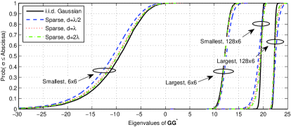
Fig. 2 provides the cumulative distribution function (CDF) of the smallest/largest eigenvalue of $\bf{G}\bf{G}^{*}$ for small-scale MIMO systems ($M=K=6$) and massive MIMO systems ($M=128$, $K=6$). Meanwhile, we plot the CDF of the smallest/largest eigenvalue of $\bf{G}\bf{G}^{*}$ under the ideal Gaussian channel matrix assumption as the benchmark for comparison. Clearly, the gap of eigenvalue distributions of $\bf{G}\bf{G}^{*}$ over sparse multipath channels and that under the ideal Gaussian channel matrix is negligible, and this gap is narrowed when $d$ increases. Besides, the simulated CDFs of eigenvalue distributions of $\bf{G}\bf{G}^{*}$ over sparse multipath channels conform to the experimental results provided by Fig. 6 of [1].

Refer to caption
Figure 1: |E​{𝐠p​[n]​𝐠q​[n]βˆ—/M}|𝐸subscript𝐠𝑝delimited-[]𝑛subscriptπ π‘žsuperscriptdelimited-[]𝑛𝑀\!|E\left\{{{{\bf{g}}_{p}}[n]{{\bf{g}}_{q}}{{[n]}^{*}}/M}\right\}| and var​{𝐠p​[n]​𝐠q​[n]βˆ—/M}varsubscript𝐠𝑝delimited-[]𝑛subscriptπ π‘žsuperscriptdelimited-[]𝑛𝑀{\rm{var}}\left\{{{{\bf{g}}_{p}}[n]{{\bf{g}}_{q}}{{[n]}^{*}}/M}\right\} against $M$ andΒ d𝑑d.

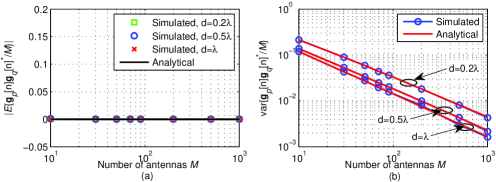
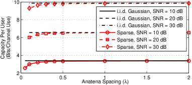
Fig. 3 shows the capacity of massive MIMO systems with $\!\!\!M\!\!\!\!=\!\!\!128$ and $\!K\!\!\!=\!\!\!16$ over sparse multipath channels and that under the ideal Gaussian channel matrix assumption. The capacity gap between massive MIMO systems over realistic sparse multipath channels and that under the ideal Gaussian channel matrix assumption is small, and this gap is narrowed when $d$ becomes large, since the inter-user interference is reduced when $d$ becomes large as confirmed in Fig. 1. Note that we do not consider the antenna coupling, which may further degrade the attainable capacity when $d$ is small. The small capacity loss conforms to the experimental results that the capacity of implemented massive MIMO always approaches the capacity under favorable propagation conditionΒ [1]. Besides, the small capacity loss implies that we may realize BS antenna array with small form factor (e.g., $\!d<\!0.5\lambda$) at the cost of a small capacity loss if the antenna coupling can be settled well.

V Conclusions

This paper has investigated the propagation condition and system capacity of massive MIMO over realistic sparse channels with SCS in both time domain and angle domain. We have proven the equivalence between the favorable propagation condition desired by massive MIMO and realistic channels with SCS. Specifically, we have derived the first and second-order moments of the inner product of different channel vectors over sparse multipath channels. Moreover, the asymptotic orthogonality of channel vectors over massive channels with SCS is proven. This proof indicates that the capacity of massive MIMO over realistic massive MIMO channels with SCS can approach that of the ideal Gaussian channel matrix assumption when the number of BS antennas is unlimited. The asymptotic orthogonality of channel vectors has been verified by comparing the simulated and analytical first and second-order moments of the inner product of channel vectors. Moreover, the simulated condition number of channel matrix and achievable capacity of massive MIMO systems over sparse MIMO channels are consistent with experimental results. The negligible capacity gap between massive MIMO over realistic sparse channels and that under the ideal Gaussian channel matrix assumption may inspire us to realize massive MIMO with better performance by exploiting the channel sparsity.

Refer to caption
Figure 2: CDFs of smallest/largest eigenvalue of $\bf{G}\bf{G}^{*}$ in MIMO systems.
Refer to caption
Figure 3: Comparison of capacity per user (bits/channel use) against the antenna spacing $\lambda$ in the massive MIMO system with $M=128$ and $K=16$.

References

  • [1] F. Rusek, et al.Β β€œScaling up MIMO: Opportunities and challenges with very large arrays,” IEEE Signal Process. Mag., vol. 30, no. 1, pp. 40-60, Jan. 2013.
  • [2] A. Pitarokoilis, S. K. Mohammed, and E. G. Larsson, β€œOn the optimality of single-carrier transmission in large-scale antenna systems,” IEEE Wireless Commun. Lett., vol. 1, no. 4, pp. 276-279, Aug. 2012.
  • [3] T. Santos, J. Kredal, P. Almers, F. Tufvesson, and A. Molisch, β€œModeling the ultra-wideband outdoor channel: Measurements and parameter extraction method,” IEEE Trans. Wireless. Commun., vol. 9, no. 1, pp. 282-290, Jan. 2010.
  • [4] Y. Barbotin and M. Vetterli, β€œEstimation of sparse MIMO channels with common support,” IEEE Trans. Commun., vol. 60, no. 12, pp. 3705-3716, Dec. 2012.
  • [5] Z. Gao, L. Dai, C. Yuen, and Z. Wang, β€œSuper-resolution sparse MIMO-OFDM channel estimation based on spatial and temporal correlations,” IEEE Commun. Lett., vol. 18, no. 7, pp. 1266-1269, July 2014.
  • [6] C. Qi and L. Wu, β€œUplink channel estimation for massive MIMO systems exploring joint channel sparsity,” Electron. Lett., vol. 50, no. 23, pp. 1770-1772, Nov. 2014.
  • [7] C. Masouros and M. Matthaiou, β€œSpace-constrained massive MIMO: Hitting the wall of favorable propagation,” IEEE Commun. Lett., vol. 19, no. 5, pp. 771-774, May 2015.
  • [8] N. Kolomvakis, M. Matthaiou, and M. Coldrey, β€œMassive MIMO in sparse channels,” in Proc. IEEE SPAWC 2014 (Toronto, Canada), Jun. 2014. pp. 21-25.
  • [9] 3GPP Technical Specification 36.211. Evolved Universal Terrestrial Radio Access (E-UTRA); Physical Channels and Modulation.
  • [10] M. Abramowitz and I. A. Stegun, Handbook of Mathematical Functions with Formulas, Graphs, and Mathematical Tables, U.S. Government Printing Office, 1964.