Incorporating exact two-body propagators for zero-range interactions into $N$-body Monte Carlo simulations

Abstract

Ultracold atomic gases are, to a very good approximation, described by pairwise zero-range interactions. This paper demonstrates that $N$-body systems with two-body zero-range interactions can be treated reliably and efficiently by the finite temperature and ground state path integral Monte Carlo approaches, using the exact two-body propagator for zero-range interactions in the pair product approximation. Harmonically trapped one- and three-dimensional systems are considered. A new propagator for the harmonically trapped two-body system with infinitely strong zero-range interaction, which may also have applications in real time evolution schemes, is presented.

I Introduction

Systems with two-body zero-range interactions constitute important models in physics. Although realistic two-body interactions do typically have a finite range, results for systems with zero-range interactions provide a starting point for understanding complicated few- and many-body dynamics. In 1934 Fermi (1934), Fermi used the zero-range model in quantum mechanical calculations to explain the scattering of slow neutrons off bound hydrogen atoms. Nowadays, the two-body contact interaction is discussed in elementary quantum texts Claude Cohen-Tannoudji . It has, e.g., been used to gain insights into the correlations of molecules, such as $\text{H}_{2}^{+}$ and $\text{H}_{2}$, and to model atom-laser interactions Demkov and Ostrovskiĭ (1988); Krstić et al. (1991); Manakov et al. (2000).

In the 60s Girardeau (1960); Lieb and Liniger (1963); Gaudin (1967); Yang (1967); Yang and Yang (1969), zero-range interactions were used extensively to model strongly-interacting one-dimensional systems at zero and finite temperature. Many of these models are relevant to electronic systems where the screening of the long-range Coulomb interactions leads to effectively short-range interactions Jones and March (1985). More recently, ultracold atomic gases interacting through two-body van der Waals potentials have been, in the low temperature regime, modeled successfully using zero-range interactions Bloch et al. (2008); Dalfovo et al. (1999); Giorgini et al. (2008). One-, two-, and three-dimensional systems have been considered.

While zero-range interactions have been at the heart of a great number of discoveries, including the Efimov effect Efimov (1970); Fedorov et al. (1994); Braaten and Hammer (2006), their incorporation into numerical schemes is not always straightforward. Loosely speaking, the challenge in using zero-range interactions in numerical schemes that work with continuous spatial coordinates stems from the fact that we, in general, do not know how to incorporate the boundary conditions implied by the zero-range potential into numerical approaches at the four- and higher-body level.

This paper discusses an approach that allows for the use of zero-range potentials in many-body simulations. We work in position space and consider a system with fixed number of particles. We develop a scheme to incorporate pairwise zero-range interactions into $e^{-\tau H}$ directly, where $H$ is the system Hamiltonian. The quantity $e^{-\tau H}$ is of fundamental importance. If $\tau$ is identified with $1/(k_{B}T)$, where $k_{B}$ and $T$ denote the Boltzmann constant and temperature, respectively, then $e^{-\tau H}$ is the density matrix for the system at finite temperature. Knowing the density matrix, the thermodynamic properties can be calculated. If, on the other hand, $\tau$ is identified with $it/\hbar$, where $t$ denotes the real time, then $e^{-\tau H}$ can be interpreted as the real time propagator and be used to calculate dynamic properties. Throughout this paper, we refer to $\tau$ as imaginary time, keeping in mind that $\tau$ carries units of $1/\text{energy}$ and that $\tau$ can be associated with inverse temperature or real time.

The remainder of this paper is organized as follows. Section II reviews the pair product approximation, which relates the many-body propagator to the two-body propagator. Section III derives the two-body propagator for various systems with zero-range interactions. Sections IV and V demonstrate that the two-body zero-range propagators yield reliable results if used in one- and three-dimensional path integral Monte Carlo (PIMC) Ceperley (1995); Boninsegni (2005); Krauth (2006) and path integral ground state (PIGS) Ceperley (1995); Hetényi et al. (1999); Sarsa et al. (2000); Cuervo et al. (2005); Rossi et al. (2009) simulations of trapped $N$-atom systems. The performance and implementation details will be discussed. While the free-space zero-range propagators have been reported in the literature Gaveau and Schulman (1986); Blinder (1988); Lawande and Bhagwat (1988); Wódkiewicz (1991), the zero-range propagators for the harmonically trapped system with infinite coupling constant are, to the best of our knowledge, new. Finally, Sec. VI concludes.

II $N$-body density matrix

We consider $N$ particles with mass $m_{j}$ and position vector $\mathbf{r}_{j}$ $(j=1,\dots,N)$ interacting via a sum of zero-range potentials with interaction strength $g$. The Hamiltonian $H$ of the system can be written as

$$H=\sum_{j=1}^{N}H_{j}^{\text{sp}}+\sum_{j<k}^{N}V_{jk},$$ (1)

where $H_{j}^{\text{sp}}$ denotes the non-interacting single-particle Hamiltonian of the $j$th particle and $V_{jk}$ the two-body potential between the $j$th and $k$th particle. In the following, it will be convenient to separate the Hamiltonian $H_{jk}$, where $H_{jk}=H_{j}^{\text{sp}}+H_{k}^{\text{sp}}+V_{jk}$, of atoms $j$ and $k$ into relative and center of mass pieces, $H_{jk}=H_{jk}^{\text{rel}}+H_{jk}^{\text{c.m.}}$, where $H_{jk}^{\text{rel}}$ depends on the relative vector $\mathbf{r}_{jk}$, and $H_{jk}^{\text{c.m.}}$ on the center of mass vector $\mathbf{r}_{jk}^{\text{c.m.}}$, $\mathbf{r}_{jk}=\mathbf{r}_{j}-\mathbf{r}_{k}$ and $\mathbf{r}_{jk}^{\text{c.m.}}=(m_{j}\mathbf{r}_{j}+m_{k}\mathbf{r}_{k})/(m_{j}+m_{k})$. Below, the non-interacting two-particle system will serve as a reference system and we define $H_{jk}^{0}=H_{j}^{\text{sp}}+H_{k}^{\text{sp}}$ and $H_{jk}^{0}=H_{jk}^{\text{rel},0}+H_{jk}^{\text{c.m.}}$.

The $N$-particle density matrix $\rho_{\text{tot}}(\mathbf{R},\mathbf{R}^{\prime};\tau)$ in position space can be written as

$$\rho_{\text{tot}}(\mathbf{R},\mathbf{R}^{\prime};\tau)=\Braket{\mathbf{R}}{e^{-\tau H}}{\mathbf{R}^{\prime}},$$ (2)

where $\mathbf{R}=(\mathbf{r}_{1},\dots,\mathbf{r}_{N})$ and $\mathbf{R}^{\prime}=(\mathbf{r}_{1}^{\prime},\dots,\mathbf{r}_{N}^{\prime})$ collectively denote the coordinates of the $N$-particle system. For sufficiently small $\tau$, $\rho_{\text{tot}}(\mathbf{R},\mathbf{R}^{\prime};\tau)$ can be constructed using the pair-product approximation Ceperley (1995),

$$\rho_{\text{tot}}(\mathbf{R},\mathbf{R}^{\prime};\tau)\approx\left(\prod_{j=1}^{N}\rho^{\text{sp}}(\mathbf{r}_{j},\mathbf{r}^{\prime}_{j};\tau)\right)\times$$

$$\left(\prod_{j<k}^{N}\bar{\rho}^{\text{rel}}(\mathbf{r}_{jk},\mathbf{r}^{\prime}_{jk};\tau)\right),$$ (3)

where $\bar{\rho}^{\text{rel}}(\mathbf{r}_{jk},\mathbf{r}^{\prime}_{jk};\tau)$ denotes the normalized pair density matrix,

$$\bar{\rho}^{\text{rel}}(\mathbf{r}_{jk},\mathbf{r}^{\prime}_{jk};\tau)=\frac{\rho^{\text{rel}}(\mathbf{r}_{jk},\mathbf{r}^{\prime}_{jk};\tau)}{\rho^{\text{rel},0}(\mathbf{r}_{jk},\mathbf{r}^{\prime}_{jk};\tau)},$$ (4)

and $\rho^{\text{rel}}(\mathbf{r}_{jk},\mathbf{r}^{\prime}_{jk};\tau)$ and $\rho^{\text{rel},0}(\mathbf{r}_{jk},\mathbf{r}^{\prime}_{jk};\tau)$ the relative density matrices of the interacting and non-interacting two-body systems,

$$\rho^{\text{rel}}(\mathbf{r}_{jk},\mathbf{r}^{\prime}_{jk};\tau)=\Braket{\mathbf{r}_{jk}}{e^{-\tau H_{jk}^{\text{rel}}}}{\mathbf{r}^{\prime}_{jk}}$$ (5)

and

$$\rho^{\text{rel},0}(\mathbf{r}_{jk},\mathbf{r}^{\prime}_{jk};\tau)=\Braket{\mathbf{r}_{jk}}{e^{-\tau H_{jk}^{\text{rel},0}}}{\mathbf{r}^{\prime}_{jk}}.$$ (6)

In Eq. (3), $\rho^{\text{sp}}(\mathbf{r}_{j},\mathbf{r}^{\prime}_{j};\tau)$ denotes the single-particle density matrix,

$$\rho^{\text{sp}}(\mathbf{r}_{j},\mathbf{r}^{\prime}_{j};\tau)=\Braket{\mathbf{r}_{j}}{e^{-\tau H_{j}^{\text{sp}}}}{\mathbf{r}_{j}^{\prime}}.$$ (7)

The key idea behind Eq. (3) is that the one- and two-body density matrices can, often times, be calculated analytically. Indeed, the non-interacting propagator is known in the literature both for the free-space and harmonically trapped systems Pathria (1996); Ceperley (1995). Moreover, the eigen energies and eigen states of the Hamiltonian $H_{jk}^{\text{rel}}$ have, for a class of two-body interactions, compact expressions, which enables the analytical evaluation of the relative two-body density matrix in certain cases (see Sec. III).

It should be noted that the pair product approximation is only valid in the small $\tau$ limit since it does not account for three- and higher-body correlations. For the real time dynamics, this means that the time step is limited by the importance of $N$-body ($N>2$) correlations. If $\tau$ is identified with $1/(k_{B}T)$, the pair product approximation is limited to high temperature. In this case, the pair product approximation is analogous to a virial expansion that includes the second-order but not the third-order virial coefficient Huang (1987).

III two-body relative density matrix

In the following, we consider one- and three-dimensional systems, without and with external harmonic confinement, and discuss the evaluation of the relative density matrix for zero-range interactions. For notational simplicity, we leave off the subscripts $j$ and $k$ throughout this section, i.e., we denote the relative distance vector by $\mathbf{r}$ for the three-dimensional system and $x$ for the one-dimensional system, respectively, and the relative part of the two-body Hamiltonian by $H^{\text{rel}}$.

III.1 One-dimensional system

The complete set of bound and continuum states of $H^{\text{rel}}$ is spanned by $\psi_{n}$ with eigen energies $E_{n}$ and $\psi_{k}$ with energies $\hbar^{2}k^{2}/(2\mu)$, where $\mu$ denotes the reduced two-body mass and $k$ the relative scattering wave vector. If the $\psi_{n}$ and $\psi_{k}$ are normalized according to

$$\int\!\psi_{n}^{*}(x)\psi_{n^{\prime}}(x)\,\mathrm{d}x=\delta_{nn^{\prime}}$$ (8)

and

$$\int\!\psi_{k}^{*}(x)\psi_{k^{\prime}}(x)\,\mathrm{d}x=\delta(k-k^{\prime}),$$ (9)

then the relative density matrix $\rho^{\text{rel}}(x,x^{\prime};\tau)$ can be written as Pathria (1996)

$$\rho^{\text{rel}}(x,x^{\prime};\tau)=\sum_{n}\psi_{n}^{*}(x)e^{-\tau E_{n}}\psi_{n}(x^{\prime})+$$

$$\int_{0}^{\infty}\!\psi_{k}^{*}(x)e^{-\tau\hbar^{2}k^{2}/(2\mu)}\psi_{k}(x^{\prime})\,\mathrm{d}k.$$ (10)

Free-space system: The relative Hamiltonian for the free-space system with zero-range interaction can be written as

$$H^{\text{rel}}=-\frac{\hbar^{2}}{2\mu}\frac{\partial^{2}}{\partial x^{2}}+g\delta(x),$$ (11)

where $g$ denotes the coupling constant of the $\delta$-function potential. For positive $g$, the Hamiltonian given in Eq. (11) does not support a bound state and the corresponding energy spectrum is continuous. The symmetric and anti-symmetric scattering states with energy $\hbar^{2}k^{2}/(2\mu)$ read 

$$\psi_{k}^{s}(x) = \frac{1}{\sqrt{\pi}}\sin\left(k|x|+\delta(k)\right)$$ (12)

and

$$\psi_{k}^{a}(x) = \frac{1}{\sqrt{\pi}}\sin(kx),$$ (13)

respectively; $\delta(k)=\arctan\left[\hbar^{2}k/(g\mu)\right]$ is the phase shift. For negative $g$, the Hamiltonian additionally supports a bound state with symmetric wave function

$$\psi_{0}^{s}(x) = \sqrt{\frac{\mu|g|}{\hbar^{2}}}e^{-\mu|gx|/\hbar^{2}}$$ (14)

and energy $-g^{2}\mu/(2\hbar^{2})$. Integrating over the symmetric and anti-symmetric scattering states, and adding, for negative $g$, the additional bound state, one finds the normalized relative density matrix $\bar{\rho}_{\text{1D,free}}^{\text{rel}}$ Gaveau and Schulman (1986); Blinder (1988); Lawande and Bhagwat (1988); Wódkiewicz (1991),

$$\bar{\rho}_{\text{1D,free}}^{\text{rel}}(x,x^{\prime};\tau)=1-\exp\left(-\frac{\mu\left(xx^{\prime}+\left|xx^{\prime}\right|\right)}{\tau\hbar^{2}}\right)\times$$

$$\sqrt{\frac{\pi\mu\tau}{2}}\frac{g}{\hbar}\operatorname{erfc}(u)\exp(u^{2}),$$ (15)

where $u=\mu\left(\left|x^{\prime}\right|+\left|x\right|+g\tau\right)/\sqrt{2\mu\tau\hbar^{2}}$ and $\operatorname{erfc}$ is the complementary error function. We emphasize that Eq. (15) holds for positive and negative $g$. The corresponding relative non-interacting density matrix reads

$$\rho_{\text{1D,free}}^{\text{rel},0}(x,x^{\prime};\tau)=\left(\frac{\mu}{2\pi\tau\hbar^{2}}\right)^{1/2}\exp\left(-\frac{\mu(x-x^{\prime})^{2}}{2\tau\hbar^{2}}\right).$$ (16)

The free-space propagator given in Eq. (15) was employed in a PIMC study of the harmonically trapped spin-polarized two-component Fermi gas with negative $g$ Casula et al. (2008).

For large $|g|$, $u$ approaches $\sqrt{\mu\tau/2}g/\hbar$ and, using $\lim_{u\to\infty}\sqrt{\pi}u\operatorname{erfc}(u)\exp(u^{2})=1$, Eq. (15) reduces to

$$\bar{\rho}_{\text{1D,free}}^{\text{rel}}(x,x^{\prime};\tau)=\begin{cases}1-\exp\left(-\frac{2\mu xx^{\prime}}{\tau\hbar^{2}}\right)&\text{for $xx^{\prime}>0$}\\ 0&\text{for $xx^{\prime}\leq 0$}.\end{cases}$$ (17)

Equation (17) suggests that the relative coordinate does not change sign during the imaginary time evolution. Since the interaction strength is infinitely strong, the two particles fully reflect during any scattering process, i.e., the transmission coefficient is zero. This means that the initial particle ordering remains unchanged during the time evolution. This is a direct consequence of the Bose-Fermi duality of one-dimensional systems Girardeau (1960); Olshanii (1998); Girardeau et al. (2004). Specifically, the phase shift of the symmetric wave function given in Eq. (12) goes to zero when $|g|\to\infty$, implying that the symmetric wave functions coincide, except for an overall $\text{sgn}(x)$ factor, with the anti-symmetric scattering wave functions of non-interacting fermions. The implications of the Bose-Fermi duality for Monte Carlo simulations of $N$-body systems with infinite $g$ is discussed in Sec. IV.

Trapped system: For two particles in a harmonic trap, the system Hamiltonian reads

$$H^{\text{rel}}=-\frac{\hbar^{2}}{2\mu}\frac{\partial^{2}}{\partial x^{2}}+g\delta(x)+\frac{1}{2}\mu\omega^{2}x^{2},$$ (18)

where $\omega$ denotes the angular trapping frequency. The energy spectrum of $H^{\text{rel}}$ is discrete and the eigen energies and eigen functions are known analytically in compact form Busch et al. (1998). These solutions can be used to evaluate Eq. (10) numerically. The corresponding relative non-interacting density matrix reads

$$\rho_{\text{1D,trap}}^{\text{rel},0}(x,x^{\prime};\tau)=\left[2\pi\sinh(\tau\hbar\omega)a_{\text{ho}}^{2}\right]^{-1/2}\times$$

$$\exp\left(-\frac{(x^{2}+x^{\prime 2})\cosh(\tau\hbar\omega)-2xx^{\prime}}{2\sinh(\tau\hbar\omega)a_{\text{ho}}^{2}}\right),$$ (19)

where $a_{\text{ho}}$ denotes the harmonic oscillator length, $a_{\text{ho}}=\sqrt{\hbar/(\mu\omega)}$. For fixed $\tau$ and finite $g$, one can then tabulate $\bar{\rho}_{\text{1d,trap}}^{\text{rel}}(x,x^{\prime};\tau)$ for discrete $x$ and $x^{\prime}$ using Eq. (10) and use a two-dimensional interpolation during the $N$-body simulation. The infinite sum in Eq. (10) can be truncated by omitting terms with $n>n_{\text{max}}$, where $n_{\text{max}}$ is chosen such that the Boltzmann factor fulfills the inequality $e^{-\tau E_{n}}\ll e^{-\tau E_{0}}$. The value of $n_{\text{max}}$ depends on the time step: smaller $\tau$ require larger $n_{\text{max}}$.

For infinite $g$, we were able to derive a compact analytical expression for $\bar{\rho}_{\text{1D,trap}}^{\text{rel}}(x,x^{\prime};\tau)$. As $g$ goes to infinity, the probability distribution of each even state coincides with that of an odd state, i.e., the system is fermionized. The complete set of even and odd eigen states for $g=\infty$ can be written as

$$\psi_{n}^{s}(x) = \phi_{n}(|x|)$$ (20)

and

$$\psi_{n}^{a}(x) = \phi_{n}(x),$$ (21)

where $\phi_{n}(x)$ is the non-interacting harmonic oscillator wave function,

$$\phi_{n}(x)=(\sqrt{\pi}2^{n}n!a_{\text{ho}})^{-1/2}e^{-x^{2}/(2a_{\text{ho}}^{2})}H_{n}(x/a_{\text{ho}}),$$ (22)

$H_{n}(x)$ denotes the Hermite polynomial of order $n$, and $n$ takes the values $1,3,5,7,\dots$. The corresponding energies are $E_{n}=(n+1/2)\hbar\omega$ for both the symmetric and anti-symmetric states, i.e., each energy level is two-fold degenerate. Using Eqs. (20) and (21) in Eq. (10) and evaluating the infinite sum analytically, we find

$$\bar{\rho}_{\text{1D,trap}}^{\text{rel}}(x,x^{\prime};\tau)=\begin{cases}1-\exp\left(-\frac{2xx^{\prime}}{\sinh(\tau\hbar\omega)a_{\text{ho}}^{2}}\right)&\text{for $xx^{\prime}>0$}\\ 0&\text{for $xx^{\prime}\leq 0$}.\end{cases}$$ (23)

For $\tau\hbar\omega\ll 1$, i.e., when the trap energy scale is much smaller than $1/\tau$, the trap propagator [Eq. (23)] equals the free-space propagator [Eq. (17)].

To test the one-dimensional propagators for infinite $g$, we consider the Hamiltonian given in Eq. (18) and prepare an initial state using a linearly discretized spatial grid. Our aim is to determine the ground state wave function and energy by imaginary time propagation. Two approaches are used. First, the initial state is propagated using the exact trap propagators [see Eqs. (23) and (19)]. In this case, the error originates solely from the discretization of the spatial degree of freedom; indeed, we find that the energy approaches the exact ground state energy quadratically with decreasing grid spacing $\delta x$. Second, the initial state is propagated using the free-space propagator [see Eqs. (17) and (16)]. We apply the Trotter formula Trotter (1959) and move half of the trap potential to the left and half to the right of the free-space Hamiltonian. This is known as the primitive approximation Ceperley (1995), which is expected to yield a quadratic time step error since the trap potential does not commute with the free-space Hamiltonian. The error is found to scale quadratically with both the time step and the grid spacing. For $\tau=(50\hbar\omega)^{-1}$, $\delta x=\sqrt{2}a_{\text{ho}}/40$, and $x_{\text{max}}=-x_{\text{min}}=4\sqrt{2}a_{\text{ho}}$, where $x_{\text{min}}\leq x\leq x_{\text{max}}$, we obtain energies that deviate by $2.4\times 10^{-5}\hbar\omega$ and $2\times 10^{-12}\hbar\omega$ for the free-space propagator and the trap propagator, respectively, from the exact ground state energy of $3\hbar\omega/2$.

III.2 Three-dimensional system

Because the $s$-wave zero-range potential is spherically symmetric, the relative orbital angular momentum operator commutes with the relative Hamiltonian. Correspondingly, we label the bound states $\psi_{nlm}$ with eigen energies $E_{nl}$ and the continuum states $\psi_{klm}$ with energies $\hbar^{2}k^{2}/(2\mu)$ by the relative orbital angular momentum quantum number $l$ and the projection quantum number $m$. If the $\psi_{nlm}$ and $\psi_{klm}$ are normalized according to

$$\int\!\psi_{nlm}^{*}(\mathbf{r})\psi_{n^{\prime}l^{\prime}m^{\prime}}(\mathbf{r})\,\mathrm{d}\mathbf{r}=\delta_{nn^{\prime}}\delta_{ll^{\prime}}\delta_{mm^{\prime}}$$ (24)

and

$$\int\!\psi_{klm}^{*}(\mathbf{r})\psi_{k^{\prime}l^{\prime}m^{\prime}}(\mathbf{r})\,\mathrm{d}\mathbf{r}=\delta(k-k^{\prime})\delta_{ll^{\prime}}\delta_{mm^{\prime}},$$ (25)

the relative density matrix $\rho^{\text{rel}}(\mathbf{r},\mathbf{r}^{\prime};\tau)$ can be written as Pathria (1996)

$$\rho^{\text{rel}}(\mathbf{r},\mathbf{r}^{\prime};\tau)=\sum_{nlm}\psi_{nlm}^{*}(\mathbf{r})e^{-\tau E_{nl}}\psi_{nlm}(\mathbf{r}^{\prime})+$$

$$\sum_{lm}\int_{0}^{\infty}\!\psi_{klm}^{*}(\mathbf{r})e^{-\tau\hbar^{2}k^{2}/(2\mu)}\psi_{klm}(\mathbf{r}^{\prime})\,\mathrm{d}k.$$ (26)

Free-space system: The Hamiltonian of the three-dimensional system in free space reads

$$H^{\text{rel}}=-\frac{\hbar^{2}}{2\mu}\nabla_{\mathbf{r}}^{2}+\frac{2\pi\hbar^{2}a_{s}}{\mu}\delta^{(3)}(\mathbf{r})\frac{\partial}{\partial r}r,$$ (27)

where $a_{s}$ is the $s$-wave scattering length. The second term on the right hand side of Eq. (27) is the regularized two-body zero-range pseudopotential Huang and Yang (1957). The $l>0$ continuum states read

$$\psi_{klm}(\mathbf{r})=i^{l}\sqrt{\frac{2}{\pi}}kj_{l}(kr)Y_{lm}(\hat{\mathbf{r}}),$$ (28)

where the $j_{l}$ and $Y_{lm}$ denote spherical Bessel functions of the first kind and spherical harmonics, respectively. The continuum states for the $s$-wave channel read

$$\psi_{k00}(\mathbf{r})=\frac{1}{\sqrt{2}\pi r}\sin(kr+\delta_{s}(k)),$$ (29)

where $\delta_{s}(k)=\arctan(-a_{s}k)$ is the $s$-wave phase shift. For positive $a_{s}$, there exists an $s$-wave bound state with eigen function $\psi_{000}(\mathbf{r})=1/\sqrt{2\pi a_{s}r^{2}}\exp(-r/a_{s})$ and eigen energy $-\hbar^{2}/(2\mu a_{s}^{2})$. As is evident from the above eigen states, only the $s$-wave states are affected by the interactions. Thus, we construct the relative interacting density matrix $\rho_{\text{3D,free}}^{\text{rel}}$ by writing the non-interacting relative density matrix $\rho_{\text{3D,free}}^{\text{rel},0}$ and subtracting from it the non-interacting $s$-wave contribution and adding to it the $s$-wave contribution for finite $a_{s}$.

For negative $a_{s}$, there exist only continuum states and the density matrix can be expressed as

$$\rho_{\text{3D,free}}^{\text{rel}}(\mathbf{r},\mathbf{r}^{\prime};\tau)= \rho_{\text{3D,free}}^{\text{rel},0}(\mathbf{r},\mathbf{r}^{\prime};\tau)+$$

$$\int_{0}^{\infty}\!e^{-\frac{\tau\hbar^{2}k^{2}}{2\mu}}\frac{1}{2\pi^{2}rr^{\prime}}[ \sin(kr+\delta_{s}(k))\sin(kr^{\prime}+\delta_{s}(k))-$$

$$\sin(kr)\sin(kr^{\prime})]\,\mathrm{d}k,$$ (30)

where the non-interacting relative density matrix reads

$$\rho_{\text{3D,free}}^{\text{rel,0}}(\mathbf{r},\mathbf{r}^{\prime};\tau)=(2\pi\hbar^{2}\tau/\mu)^{-3/2}e^{-\mu(\mathbf{r}-\mathbf{r}^{\prime})^{2}/(2\hbar^{2}\tau)}.$$ (31)

The integral in Eq. (30) can be done analytically  and the normalized relative density matrix reads Lawande and Bhagwat (1988); Wódkiewicz (1991)

$$\bar{\rho}_{\text{3D,free}}^{\text{rel}}(\mathbf{r},\mathbf{r}^{\prime};\tau)=1+\frac{\hbar^{2}\tau}{\mu rr^{\prime}}\exp\left(-\frac{\mu rr^{\prime}(1+\cos\theta)}{\hbar^{2}\tau}\right)\times$$

$$\left(1+\frac{\hbar}{a_{s}}\sqrt{\frac{\pi\tau}{2\mu}}\operatorname{erfc}(v)\exp(v^{2})\right),$$ (32)

where $\cos\theta=\mathbf{r}\cdot\mathbf{r}^{\prime}/(rr^{\prime})$ and $v=[r+r^{\prime}-\tau\hbar^{2}/(\mu a_{s})]/\sqrt{2\tau\hbar^{2}/\mu}$. Adding the bound state contribution to Eq. (30) [see the first term on the right hand side of Eq. (26)] for positive $a_{s}$, one finds Eq. (32), i.e., the same propagator as for negative $a_{s}$ Wódkiewicz (1991).

For $|a_{s}|=\infty$, Eq. (32) simplifies to

$$\bar{\rho}_{\text{3D,free}}^{\text{rel}}(\mathbf{r},\mathbf{r}^{\prime};\tau)=1+\frac{\hbar^{2}\tau}{\mu rr^{\prime}}\exp\left(-\frac{\mu rr^{\prime}(1+\cos\theta)}{\hbar^{2}\tau}\right).$$ (33)

This propagator was recently used in a proof-of-principle diffusion Monte Carlo study of the homogeneous two-component Fermi gas at unitarity with zero-range interactions Pessoa et al. .

Trapped system: The Hamiltonian for two particles in a spherically symmetric harmonic trap with $s$-wave scattering length $a_{s}$ reads

$$H^{\text{rel}}=-\frac{\hbar^{2}}{2\mu}\nabla_{\mathbf{r}}^{2}+\frac{1}{2}\mu\omega^{2}\mathbf{r}^{2}+\frac{2\pi\hbar^{2}a_{s}}{\mu}\delta^{(3)}(\mathbf{r})\frac{\partial}{\partial r}r.$$ (34)

The non-interacting relative density matrix reads

$$\rho_{\text{3D,trap}}^{\text{rel},0}(\mathbf{r},\mathbf{r}^{\prime};\tau)=a_{\text{ho}}^{-3}\left[2\pi\sinh(\tau\hbar\omega)\right]^{-3/2}\times$$

$$\exp\left({-\frac{(\mathbf{r}^{2}+\mathbf{r}^{\prime 2})\cosh(\tau\hbar\omega)-2\mathbf{r}\cdot\mathbf{r}^{\prime}}{2\sinh(\tau\hbar\omega)a_{\text{ho}}^{2}}}\right).$$ (35)

Similar to the free-space case, the relative interacting density matrix is obtained from the non-interacting density matrix with the difference of the $s$-wave eigen states and energies of the interacting and non-interacting systems added. For finite $a_{s}$, we were not able to evaluate the infinite sum analytically. Because of the rotational invariance, the infinite sum depends only on $r$ and $r^{\prime}$ (and not the direction of the vectors $\mathbf{r}$ and $\mathbf{r}^{\prime}$), allowing for an efficient tabulation of the reduced relative density matrix. For infinitely large $a_{s}$, we find an analytical expression. In this case, the bound state wave functions that are affected by the $\delta$-function interaction can be written as $\sqrt{2}\phi_{n}(r)/\sqrt{4\pi r^{2}}$, where the $\phi_{n}(r)$ are defined in Eq. (22) with $x$ replaced by $r$ and $n=0,2,4,\dots$ The relative two-body density matrix reads

$$\rho_{\text{3D,trap}}^{\text{rel}}(\mathbf{r},\mathbf{r}^{\prime};\tau)=\rho_{\text{3D,trap}}^{\text{rel},0}(\mathbf{r},\mathbf{r}^{\prime};\tau)+$$

$$\sum_{n=0}^{\infty}e^{-\tau(n+\frac{1}{2})\hbar\omega}\frac{(-1)^{n}}{2\pi rr^{\prime}}\phi_{n}^{*}(r)\phi_{n}(r^{\prime}),$$ (36)

where the even $n$ terms in the sum over $n$ come from the $s$-wave states that are affected by the interactions and the odd $n$ terms come from the $s$-wave states of the non-interacting system. Performing the infinite sum, we find for the normalized relative density matrix

$$\bar{\rho}_{\text{3D,trap}}^{\text{rel}} (\mathbf{r},\mathbf{r}^{\prime};\tau)=1+$$

$$\frac{a_{\text{ho}}^{2}}{rr^{\prime}}\sinh(\tau\hbar\omega)\exp\left(-\frac{rr^{\prime}(1+\cos\theta)}{a_{\text{ho}}^{2}\sinh(\tau\hbar\omega)}\right).$$ (37)

Setting $\tau\hbar\omega=0$, Eq. (37) reduces to Eq. (33), i.e., to the corresponding free-space expression.

Equations (17) and (33) show that the one- and three-dimensional free-space propagators for systems with infinitely large $\delta$-function strength are characterized by the length $\sqrt{\tau\hbar^{2}/\mu}$, which is proportional to the de Broglie wave length. The trap propagators for infinitely large coupling constant [see Eqs. (23) and (37)], in contrast, are characterized additionally by the harmonic oscillator length. For finite interaction strength, the coupling constant defines a second length scale for the free-space system and a third length scale for the trapped system.

IV one dimensional tests

This section incorporates the trapped two-body propagator into PIMC calculations for one-dimensional $N$-particle systems with pairwise zero-range interactions. We find that the conventional PIMC sampling approaches Ceperley (1995); Boninsegni (2005) yield an efficient and robust description of one-dimensional systems with two-body zero-range interactions.

As a first example, we consider $N$ distinguishable harmonically trapped particles with mass $m$ in one spatial dimension with pairwise zero-range interactions of infinite strength. The $N$-particle system with infinitely large interaction strength is unique in that the particle statistics becomes irrelevant for local observables. For example, the energy is the same for $N$ identical bosons, $N$ identical fermions and $N$ distinguishable particles at any temperature provided all particles interact via two-body zero-range interactions. We employ the zero-range trap propagator together with the single-particle trap propagator. Symbols in Fig.

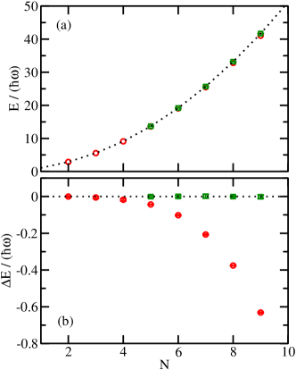
Figure 1: (Color online) PIMC results for $N$ harmonically trapped distinguishable one-dimensional particles with two-body zero-range interactions of infinite strength at temperature $T=\hbar\omega/k_{B}$. (a) The symbols show the energy obtained by the PIMC approach as a function of the number of particles $N$. For comparison, the dotted line shows the exact thermally averaged energy. (b) Symbols show the energy difference $\Delta E$ between the PIMC energies and the exact results. As a reference, the dotted line shows the $\Delta E=0$ curve. In (a) and (b), the circles and squares are calculated using $8$ and $128$ time slices, respectively.

1(a) show the PIMC energy for $N$ distinguishable particles at temperature $k_{B}T=\hbar\omega$. Circles and squares are for simulations with imaginary time step $\tau\hbar\omega=1/8$ and $1/128$, respectively. For comparison, the dotted line is calculated directly from the partition function of $N$ non-interacting fermions. Figure 1(b) shows the energy difference $\Delta E$ between the simulation and the analytical results. It can be seen that the calculations for the larger time step (circles in Fig. 1) exhibit a systematic time step error, which is found to scale quadratically with the time step $\tau$ for fixed $N$ and to originate from the pair product approximation. Since we include the two-body correlations exactly, the leading order error is expected to come from three-body correlations. Indeed, for relatively small fixed $\tau$ ($\tau^{-1}$ around $16\hbar\omega$) and varying $N$, we find that the error $\Delta E$ scales approximately linearly with the number of triples, suggesting that the error is dominated by three-body correlations with sub-leading contributions arising from four-body correlations. As the number of particles $N$ or the time step $\tau$ increase, four- and higher-body correlations become more important. This error analysis suggests that an improved propagator could be obtained if the three-body problem could be solved analytically. We note that the performance of the zero-range trap propagator for the system with infinite $g$ is quite similar to that of the free-space propagator using the second- or fourth-order Trotter decomposition. The reason is that the error is dominated by three- and higher-body correlations.

We now discuss that the simulations need to be modified to treat $N$ identical bosons or fermions with pairwise zero-range interactions of infinite strength. Equations (17) and (23) indicate that the paths for any two particles cannot cross. This implies that the permute move, implemented following the approach discussed in Ref. Cuervo et al. (2005), yields a zero acceptance probability. This is consistent with our finite $g$ simulations for $N$ identical bosons. As we change $g$ for otherwise fixed simulation parameters from small positive to large positive values, the probability of sampling the identity permutation approaches 1. The fact that particle permutations are always rejected, causes two problems for the infinite $g$ simulations. First, since the particle ordering does not change, the single particle density for the first particle differs from that of the second particle, and so on. To calculate the single particle density $\rho(x)$ of, e.g., the $N$ identical boson system, one can average the single particle density $\rho_{j}(x)$ of the $j$th particle over all $j$, $\rho(x)=N^{-1}\sum_{j=1}^{N}\rho_{j}(x)$. An analogous average can be performed for other local (closed paths) structural properties. Second, the simulation of open paths, which allow for the calculation of off-diagonal long-range order, requires that the sampling scheme be modified since open paths do allow for permutations. The two-particle density matrix $\rho(\{x_{1},x_{2}\},\{x_{2},x_{1}^{\prime}\};\tau)$, e.g., is finite if $x_{1}<x_{2}<x_{1}^{\prime}$. The calculation of non-local observables is beyond the scope of the present paper.

As a next example, we apply the zero-range trap propagator to $N=2$ and $3$ identical bosons in a harmonic trap with $g=\hbar^{2}/(\sqrt{2}\mu a_{\text{ho}})$. For the PIMC calculations, we tabulate the density matrix for the time step of interest and interpolate during the simulation. For small number of particles, we expect the zero-range trap propagator to work well even for a large time step and we use $\tau\hbar\omega=1/2$. For $k_{B}T=\hbar\omega/32$, we obtain an energy of $1.3067(1)\hbar\omega$ and $2.3880(1)\hbar\omega$ for $N=2$ and $3$, respectively. The temperature is so low that the system is essentially in the ground state. For comparison, we determined the ground state energy using the transcendental equation from Ref. Busch et al. (1998) and by solving the Lippmann-Schwinger equation Gharashi et al. (2012). The resulting ground state energies [$1.306746\hbar\omega$ and $2.3880(1)\hbar\omega$ for $N=2$ and $3$, respectively] agree within error bars with the PIMC results.

To demonstrate that the PIMC simulations describe the short-distance behavior of systems with zero-range interactions correctly, we analyze the pair distribution function $P_{12}(x)$, which is normalized to $\int_{-\infty}^{\infty}\!P_{12}(x)\,\mathrm{d}x=1$, for $N=2$ and $3$ identical bosons with finite $g$. To start with, we derive the short-distance properties of the pair distribution function $P_{12}$ for $N$ identical bosons with zero-range interactions. Using the Hellmann-Feynman theorem, the partial derivative of the energy with respect to $g$ can be related to the pair distribution function at $x=0$ Barth and Zwerger (2011),

$$P_{12}(0)=\frac{2}{N(N-1)}\frac{\partial E}{\partial g}.$$ (38)

Note that Eq. (38) is the one-dimensional analog of equating the three-dimensional adiabatic and pair relations Tan (2008). Second, from the Bethe-Peierls boundary condition of the $N$-body wave function $\Psi$ (the derivatives are taken while all other coordinates are kept fixed),

$$\frac{\partial\Psi}{\partial x_{jk}}\bigg{|}_{x_{jk}\to 0^{+}}-\frac{\partial\Psi}{\partial x_{jk}}\bigg{|}_{x_{jk}\to 0^{-}}=\frac{2\mu g}{\hbar^{2}}\Psi\bigg{|}_{x_{jk}\to 0},$$ (39)

one can derive that the slope of the pair distribution function at any temperature satisfies

$$\frac{\partial}{\partial x}P_{12}(x)\big{|}_{x\to 0^{+}}-\frac{\partial}{\partial x}P_{12}(x)\big{|}_{x\to 0^{-}}=\frac{4\mu g}{\hbar^{2}}P_{12}(x)\big{|}_{x\to 0}.$$ (40)

For identical bosons, $\partial P_{12}(x)/\partial x\big{|}_{x\to 0^{+}}$ and $\partial P_{12}(x)/\partial x\big{|}_{x\to 0^{-}}$ have the same magnitude but opposite signs.

The dashed and dotted lines in Fig. 2

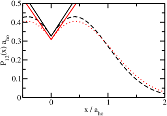
Figure 2: (Color online) PIMC results for harmonically trapped one-dimensional bosons interacting through two-body zero-range interactions with coupling constant $g=\hbar^{2}/(\sqrt{2}\mu a_{\text{ho}})$ at temperature $T=\hbar\omega/(32k_{B})$. The dashed and dotted lines show the pair distribution function obtained by the PIMC approach for $N=2$ and $3$ bosons, respectively. For comparison, the solid lines show the asymptotic short-range behavior obtained by alternative means (see text).

show $P_{12}(x)$ obtained from our PIMC simulation for $N=2$ and $3$, respectively. For comparison, the solid lines are obtained using Eqs. (38) and (40). The values of $\partial E/\partial g$ are obtained through independent energy calculations using the techniques of Refs. Busch et al. (1998); Gharashi et al. (2012). We find $P_{12}(0)=0.3266002/a_{\text{ho}}$ and $0.308245(2)/a_{\text{ho}}$ for $N=2$ and $3$, respectively. Our PIMC results agree well with the solid lines in the small $|x|$ regime, demonstrating that the PIMC approach describes the short-range behavior accurately.

V three dimensional tests

The pair distribution function of the non-interacting three-dimensional system is, unlike that of the non-interacting one-dimensional system, zero at vanishing interparticle distance. This fact leads, as we discuss now, to non-ergodic behavior unless the traditional path integral sampling methods are complemented by an additional move. To motivate the introduction of this new “pair distance move”, we consider the two-particle system.

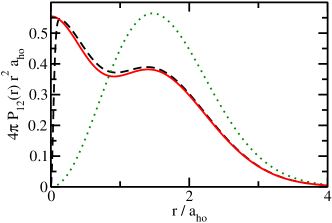
Figure 3: (Color online) Scaled pair distribution functions $4\pi P_{12}(r)r^{2}$ for two distinguishable particles of mass $m$ in a harmonic trap at $k_{B}T/(\hbar\omega)=1$. The solid and dashed lines are for two particles with infinitely large $s$-wave scattering length interacting through the zero-range potential and a Gaussian potential with effective range $r_{e}\approx 0.0861a_{\text{ho}}$, respectively. For comparison, the dotted line is for the non-interacting system.

Solid and dashed lines in Fig. 3 show the scaled pair distribution functions for two distinguishable particles with infinitely large $s$-wave scattering length in a three-dimensional harmonic trap at $k_{B}T/(\hbar\omega)=1$ interacting through a zero-range potential and a finite-range Gaussian potential with effective range $r_{e}\approx 0.0861a_{\text{ho}}$, respectively. The pair distribution function $P_{12}(r)$ is normalized according to $4\pi\int_{0}^{\infty}\!P_{12}(r)r^{2}\,\mathrm{d}r=1$. The pair distribution functions for the finite-range and zero-range potentials nearly coincide for large $r$, but differ for small $r$. The pair distribution function for the Gaussian potential drops to 0 as $r$ approaches 0 while that for the zero-range potential approaches a non-zero value.

PIMC and PIGS simulations typically use the first term on the right hand side of Eq. (3) as the “prior distribution” and the second term as the “correction”. This is suitable for $N$-body systems with two-body finite-range potentials for which the scaled pair distribution function is, as that of the non-interacting system (see the dotted line in Fig. 3 for a two-body example), zero at $r=0$. Since the prior distribution has zero probability at $r=0$, the pair distribution function of the system with zero-range interactions is not properly sampled if standard sampling schemes are used. Ergodicity is violated at $r=0$ and the probability to sample the region near $r=0$ is small. Moreover, the correction term [see Eqs. (37) and (33)] diverges as $r$ or $r^{\prime}$ go to 0. This means that the probability to sample configurations with $r\approx 0$ is small. However, if such a configuration is chosen, there is a small probability to accept a new configuration with much larger $r$, i.e., the correlation length is large. Similarly, if one uses the naive uniform distribution for the prior distribution, i.e., if one proposes a move for which all Cartesian coordinates differ by $\delta x$ from the current configuration, where $\delta x$ is a random value between $-\Delta x$ and $\Delta x$, the problems discussed above still exist.

To remedy the problems that arise if the standard sampling approaches are used, we introduce a “pair distance move” for which the prior distribution scales as $1/r^{2}$ in the pair distances. First, particles $j$ and $k$ and a bead $l$ are chosen (the coordinates for the $l$th bead are collectively denoted by $\mathbf{R}_{l}$) and the distance $r_{jk}=|\mathbf{r}_{jk}|$ and the direction $\hat{\mathbf{r}}_{jk}$ are calculated. A new vector $\mathbf{r}_{jk,\text{new}}$ that lies along $\hat{\mathbf{r}}_{jk}$ or $-\hat{\mathbf{r}}_{jk}$ is proposed, $\mathbf{r}_{jk,\text{new}}=\epsilon\hat{\mathbf{r}}_{jk}$. The quantity $\epsilon$ is written as $\epsilon=r_{jk}+\delta r$, where $\delta r$ is obtained by choosing uniformly from $-\Delta r$ to $\Delta r$. If the weight $w$,

$$w=\min[1,\frac{\rho_{\text{tot}}(\mathbf{R}_{l-1},\mathbf{R}_{l,\text{new}};\tau)\rho_{\text{tot}}(\mathbf{R}_{l+1},\mathbf{R}_{l,\text{new}};\tau)\epsilon^{2}}{\rho_{\text{tot}}(\mathbf{R}_{l-1},\mathbf{R}_{l};\tau)\rho_{\text{tot}}(\mathbf{R}_{l+1},\mathbf{R}_{l};\tau)r_{jk}^{2}}],$$ (41)

is larger than a uniform random number between 0 and 1, then the proposed move is accepted. Otherwise, it is rejected and the old configuration is kept. The value of $\Delta r$ is adjusted such that about $50\%$ of the proposed moves are accepted. It can be easily proven that detailed balance is fulfilled. Our PIMC calculations for the two-body system with zero-range interactions show that the “pair distance move” significantly improves the sampling. Without this move, the short-range behavior of the pair distribution function has a long correlation length, which increases with decreasing $\tau$. With this move, the small $r$ behavior is described accurately. The move described here is related to the compression-dilation move introduced in Ref. Piatecki and Krauth (2014). Few details were given in Ref. Piatecki and Krauth (2014) and no comparison with that approach is made in this paper.

We now demonstrate that the outlined sampling scheme provides a reliable description of Bose systems at unitarity, which have attracted a great deal of attention recently experimentally and theoretically Rem et al. (2013); Fletcher et al. (2013); Makotyn et al. (2014); Piatecki and Krauth (2014); Sykes et al. (2014); Jiang et al. (2014); Smith et al. (2014); Rossi et al. (2014). While the properties of unitary Fermi systems with zero-range interactions are fully determined by the $s$-wave scattering length Giorgini et al. (2008); Bloch et al. (2008); Blume (2012); Carlson et al. (2003); Astrakharchik et al. (2004); Werner and Castin (2006) those of Bose systems additionally depend on a three-body parameter Efimov (1970); Braaten and Hammer (2006). Specifically, if the two-body interactions are modeled by zero-range potentials, then a three-body regulator is needed to prevent the Thomas collapse of the $N$-boson ($N\geq 3$) system Thomas (1935); Braaten and Hammer (2006). Here, we utilize a purely repulsive three-body potential of the form

$$V_{\text{3b}}(R_{jkl})=\frac{C_{6}}{R_{jkl}^{6}},$$ (42)

where $R_{jkl}$ denotes the three-body hyperradius, $R_{jkl}=\sqrt{(r_{jk}+r_{jl}+r_{kl})/3}$. In the $N$-boson system, each of the $N(N-1)(N-2)/6$ triples feels the regulator, i.e., the term $\sum_{j<k<l}V_{\text{3b}}(R_{jkl})$ is added to the Hamiltonian with pairwise zero-range interactions. In the absence of an external trap, the zero temperature three-body ground state energy $E_{\text{trimer}}$ of the unitary system is set by the $C_{6}$ coefficient. The corresponding length scale is $1/\kappa$, where $\kappa=\sqrt{m|E_{\text{trimer}}|}/\hbar$ is the binding momentum.

Our goal is to determine the ground state properties of self-bound $N$-boson droplets at unitarity in the absence of an external confinement. In the context of the present paper, it would seem that our goal could be readily achieved using the PIGS approach. It turns out, however, that without a good initial trial wave function, the number of time slices needed to converge the calculations is rather large, making the simulations computationally quite expensive. Instead, one might consider performing PIMC calculations at various temperatures and extrapolating to the zero temperature limit. This approach also turns out to be computationally extensive. Our simulations pursue an alternative approach, in which the scattering states of the system are discretized in such a way that the relative ground state energy $E_{\text{cluster}}$ of the $N$-body cluster is much larger than the energy scale introduced by the discretization. We utilize a spherically symmetric harmonic trap and adjust the trapping frequency such that $|E_{\text{cluster}}|\gg\hbar\omega$. Simulations are then performed at a temperature where the Bose droplet is in the ground-state dominated liquid-phase Piatecki and Krauth (2014); Yan and Blume (2014), where the finite temperature introduces center-of-mass excitations but not excitations of the relative degrees of freedom. The temperature $T_{\text{tr}}$ at which excitations of the relative degrees of freedom become relevant can be estimated using the “combined model” introduced in Ref. Yan and Blume (2014). As we show now, this approach allows for a fairly robust determination of the $N$-boson properties at zero temperature.

We set the trap energy $\hbar\omega$ to $0.27|E_{\text{trimer}}|$ ($E_{\text{trimer}}$ is the ground state energy of the three-boson system in free space) and the temperature to $\hbar\omega/k_{B}$. These parameters provide a good compromise: First, the temperature is sufficiently low that finite temperature effects are negligible (i.e., $T<T_{\text{tr}}$ for the $N$ considered below, $N=3-9$) and high enough that convergence can be reached with the computational resources available to us. Second, the size of the $N$-boson system is smaller than the harmonic oscillator length such that structural properties such as the pair distribution function are largely unaffected by the external confinement for $N\gtrsim 5$.

Our path integral simulations use the two-body zero-range trap propagator. The repulsive three-body potentials are treated using the Trotter formula. In the second-order scheme, half of the sum of the three-body potentials is moved to the left and half to the right of the Hamiltonian $H$ that accounts for the two-body interactions and the external confinement. In the fourth-order scheme, a more involved decomposition is used Chin (1997); Jang et al. (2001). In addition to the standard moves and the “pair distance move”, we implement a move that updates the center-of-mass coordinates. The introduction of this center-of-mass move is motivated by the fact that the relative degrees of freedom are expected to be, to a good approximation, “frozen” in the ground state while low-energy center-of-mass excitations are allowed. Indeed, the center-of-mass energy is given by $E_{\text{c.m.}}=3\hbar\omega\coth(\hbar\omega/(2k_{B}T))/2$, which evaluates to $3.24593\hbar\omega$ for $T=\hbar\omega/k_{B}$, indicating that center-of-mass excitations cannot be neglected.

The squares in Fig. 4

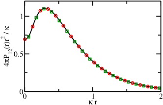
Figure 4: (Color online) Scaled pair distribution function $4\pi P_{12}(r)r^{2}$ for three identical harmonically trapped three-dimensional bosons with two-body zero-range interactions with infinitely large $s$-wave scattering length and repulsive $1/R^{6}$ three-body potential. The solid line and squares are calculated by the zero-temperature PIGS approach and the PIMC approach at $T=\hbar\omega/k_{B}$. For comparison, the circles show the scaled pair distribution function obtained by sampling the exact ground state density using the Metropolis algorithm.

show the pair distribution function calculated by the PIMC approach for three identical bosons at $T=\hbar\omega/k_{B}$. For comparison, the solid line and the circles show zero-temperature results. The solid line is calculated using the PIGS approach with a trial wave function that coincides with the exact ground state wave function  while the circles are calculated by sampling the exact zero-temperature ground state density using the Metropolis algorithm. The agreement between the three sets of calculations is very good, demonstrating (i) that excitations of the relative degrees of freedom are negligible at the temperature considered and (ii) that the path integral approaches accurately resolve the short-range behavior of the pair distribution function. The pair distribution functions shown in Fig. 4 are affected by the trap, i.e., they move to larger $r$ as the trap frequency $\omega$ is reduced. The reason is that $\hbar\omega$ is only about four times smaller than $|E_{\text{trimer}}|$. The magnitude of the $N$-boson energy $E_{\text{cluster}}$ increases rapidly with $N$ von Stecher (2010); Nicholson (2012); Gattobigio and Kievsky (2014), implying that the trap effects decrease quickly with increasing $N$, thus allowing us to extract the free-space energy $E_{\text{cluster}}$ from the finite-temperature trap energies $E_{\text{sim}}$.

Symbols in Fig. 5

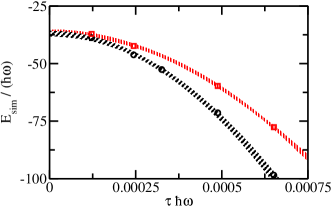
Figure 5: (Color online) PIMC energies for $N=5$ harmonically trapped three-dimensional bosons with two-body zero-range interactions with infinite scattering length and and repulsive $1/R^{6}$ three-body interaction at temperature $T=\hbar\omega/k_{B}$ as a function of the time step $\tau$. The circles (lower-lying data set) and squares (higher-lying data set) show the energy obtained using the second- and fourth-order scheme, respectively. The error bands are obtained by fitting the data for different $\tau$ intervals.

exemplarily show our PIMC energies $E_{\text{sim}}$ for the five-boson system at $T=\hbar\omega/k_{B}$ as a function of the time step $\tau$. Circles and squares are obtained using the second- and fourth-order schemes (see earlier discussion), respectively, to treat the term $\exp(-\sum_{j<k<l}\tau V_{\text{3b}}(R_{jkl}))$. The statistical errors are smaller than the symbol size. The fourth-order results display, as expected, a smaller time step dependence than the second-order results and are well described by a function of the form $c_{0}+c_{2}\tau^{2}+c_{4}\tau^{4}$, whereas the second-order results are described by a function of the form $c_{0}+c_{2}\tau^{2}$. The presence of the $\tau^{2}$ term for the fourth-order results is due to the fact that the pair product approximation neglects three- and higher-body correlations (see also Sec. IV). The shaded regions in Fig. 5 show errorbands obtained by fitting the two sets of PIMC energies for different $\tau$ intervals. The errorbars of the extrapolated zero time step energies are found to overlap. We find $E_{\text{sim}}=-37.0(1.2)\hbar\omega$ and $-36.2(1.0)\hbar\omega$ for the second- and fourth-order scheme, respectively. The free-space energy $E_{\text{cluster}}$ is then obtained by subtracting the center-of-mass energy, $E_{\text{cluster}}=E_{\text{sim}}-E_{\text{c.m.}}$.

The squares in Fig. 6

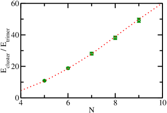
Figure 6: (Color online) Free-space $N$-boson ground state energy $E_{\text{cluster}}$ as a function of $N$ for infinitely large two-body $s$-wave scattering length. The circles with errorbars are extracted from our PIMC simulations. The dotted line shows the energies reported in Ref. von Stecher (2010).

show $E_{\text{cluster}}$ for $N=5-9$. The corresponding energies $E_{\text{sim}}$ are obtained using the fourth-order scheme with $\tau\hbar\omega\approx 0.000122$. As can be seen from Fig. 5, this energy lies within the extrapolated $\tau=0$ errorbands for $N=5$. Figure 6 scales the energy $E_{\text{cluster}}$ by the corresponding zero-temperature free-space trimer energy $E_{\text{trimer}}$ calculated by the hyperspherical coordinate approach. For comparison, the dotted line shows the $N$-boson ground state energies from Ref. von Stecher (2010) for a finite-range two-body Gaussian potential with infinitely large $s$-wave scattering length and a hardcore three-body regulator. While the model interactions differ, the agreement between the two sets of calculations is good, providing further support for the (approximate) universality of $N$-boson droplets. More detailed comparisons will be presented elsewhere .

VI conclusion

This paper discussed how to treat zero-range two-body interactions in $N$-body Monte Carlo simulations. We showed that the incorporation of the exact two-body zero-range propagator via the pair product approximation allows for an accurate description of paradigmatic strongly-interacting one- and three-dimensional model Hamiltonian.

An important aspect of the studies presented is that the strength of the contact interaction requires no renormalization since the simulations are performed using the regularized two-body zero-range pseudopotential and continuous spatial coordinates in an unrestricted Hilbert space. The fact that the interaction strength does not need to be renormalized distinguishes the simulations presented in this paper from lattice approaches Kogut (1983); Lee (2009); Drut and Nicholson (2013) and from configuration interaction approaches Esry and Greene (1999); Alhassid et al. (2008); Rontani et al. (2009).

The developments presented in this paper open a number of possibilities. The use of two-body zero-range interactions, e.g., provides direct access to the two-body Tan contact Tan (2008), without extrapolation to the zero-range limit. The two-body Tan contact is defined for systems with two-body zero-range interactions. It relates distinct physical observables such as the large momentum tail and aspects of the radio frequency spectrum, and has attracted a great deal of theoretical Werner and Castin (2012); Braaten and Platter (2008); Yu et al. (2009); Drut et al. (2011); Barth and Zwerger (2011); Doggen and Kinnunen (2013); Yan and Blume (2013) and experimental Stewart et al. (2010); Kuhnle et al. (2010, 2011); Sagi et al. (2012); Makotyn et al. (2014) interest. From the computational perspective, the adiabatic relation, which involves the change of the energy with the scattering length, and the pair relation Tan (2008); Blume and Daily (2009), which gives the probability of finding two particles at the same position, are most convenient. Earlier work applied these relations to systems with finite-range interactions and extrapolated to the zero-range limit. Using our zero-range propagators, these relations can be used directly for the determination of the Tan contact, eliminating the extrapolation step.

Acknowledgement: We thank Ebrahim Gharashi for providing the energies of three identical bosons calculated using the approach of Ref. Gharashi et al. (2012) and Maurizio Rossi for very useful comments on an earlier version of the manuscript. Support by the National Science Foundation (NSF) through Grant No. PHY-1415112 is gratefully acknowledged. This work used the Extreme Science and Engineering Discovery Environment (XSEDE), which is supported by NSF Grant No. OCI-1053575, and the WSU HPC.

References

- Fermi (1934) E. Fermi, Nuovo Cimento 11, 157 (1934).
- (2) B. Claude Cohen-Tannoudji, Quantum Mechanics, vol. 1 (Hermann, Paris).
- Demkov and Ostrovskiĭ (1988) Y. N. Demkov and V. N. Ostrovskiĭ, Zero-Range Potentials and Their Applications in Atomic Physics (Plenum Press, New York, 1988).
- Krstić et al. (1991) P. S. Krstić, D. B. Milošević, and R. K. Janev, Phys. Rev. A 44, 3089 (1991).
- Manakov et al. (2000) N. L. Manakov, M. V. Frolov, A. F. Starace, and I. I. Fabrikant, J. Phys. B 33, R141 (2000).
- Girardeau (1960) M. Girardeau, J Math. Phys. 1 (1960).
- Lieb and Liniger (1963) E. H. Lieb and W. Liniger, Phys. Rev. 130, 1605 (1963).
- Gaudin (1967) M. Gaudin, Phys. Lett. A 24, 55 (1967).
- Yang (1967) C. N. Yang, Phys. Rev. Lett. 19, 1312 (1967).
- Yang and Yang (1969) C. N. Yang and C. P. Yang, J. Math. Phys. 10 (1969).
- Jones and March (1985) W. Jones and N. H. March, Theoretical Solid State Physics, vol. 2 (Dover Publications, New York, 1985).
- Bloch et al. (2008) I. Bloch, J. Dalibard, and W. Zwerger, Rev. Mod. Phys. 80, 885 (2008).
- Dalfovo et al. (1999) F. Dalfovo, S. Giorgini, L. P. Pitaevskii, and S. Stringari, Rev. Mod. Phys. 71, 463 (1999).
- Giorgini et al. (2008) S. Giorgini, L. P. Pitaevskii, and S. Stringari, Rev. Mod. Phys. 80, 1215 (2008).
- Efimov (1970) V. Efimov, Phys. Lett. B 33, 563 (1970).
- Fedorov et al. (1994) D. V. Fedorov, A. S. Jensen, and K. Riisager, Phys. Rev. C 49, 201 (1994).
- Braaten and Hammer (2006) E. Braaten and H.-W. Hammer, Phys. Rep. 428, 259 (2006).
- Ceperley (1995) D. M. Ceperley, Rev. Mod. Phys. 67, 279 (1995).
- Boninsegni (2005) M. Boninsegni, J. Low Temp. Phys. 141, 27 (2005).
- Krauth (2006) W. Krauth, Statistical Mechanics: Algorithms and Computations, Oxford Master Series in Physics (Oxford University Press, Oxford, UK, 2006).
- Hetényi et al. (1999) B. Hetényi, E. Rabani, and B. J. Berne, J. Chem. Phys. 110, 6143 (1999).
- Sarsa et al. (2000) A. Sarsa, K. E. Schmidt, and W. R. Magro, J. Chem. Phys. 113, 1366 (2000).
- Cuervo et al. (2005) J. E. Cuervo, P.-N. Roy, and M. Boninsegni, J. Chem. Phys. 122, 114504 (2005).
- Rossi et al. (2009) M. Rossi, M. Nava, L. Reatto, and D. E. Galli, J. Chem. Phys. 131, 154108 (2009).
- Gaveau and Schulman (1986) B. Gaveau and L. S. Schulman, J. Phys. A 19, 1833 (1986).
- Blinder (1988) S. M. Blinder, Phys. Rev. A 37, 973 (1988).
- Lawande and Bhagwat (1988) S. V. Lawande and K. V. Bhagwat, Phys. Lett. A 131, 8 (1988).
- Wódkiewicz (1991) K. Wódkiewicz, Phys. Rev. A 43, 68 (1991).
- Pathria (1996) R. Pathria, Statistical Mechanics (Elsevier, Amsterdam, 1996).
- Huang (1987) K. Huang, Statistical Mechanics, 2nd ed. (Wiley, New York, 1987).
- Note (1) Equation (9) is to be interpreted as follows: and (due to symmetry).
- Casula et al. (2008) M. Casula, D. M. Ceperley, and E. J. Mueller, Phys. Rev. A 78, 033607 (2008).
- Olshanii (1998) M. Olshanii, Phys. Rev. Lett. 81, 938 (1998).
- Girardeau et al. (2004) M. D. Girardeau, H. Nguyen, and M. Olshanii, Opt. Commun. 243, 3 (2004).
- Busch et al. (1998) T. Busch, B.-G. Englert, K. Rzażewski, and M. Wilkens, Found. Phys. 28, 549 (1998).
- Trotter (1959) H. F. Trotter, Proc. Amer. Math. Soc. 10, 545 (1959).
- Huang and Yang (1957) K. Huang and C. N. Yang, Phys. Rev. 105, 767 (1957).
- Note (2) See entry 3.954 of I. S. Gradshteyn and I. M. Ryzhik, Table of Integrals, Series, and Products, 6th Ed., Academic Press.
- (39) R. Pessoa, S. A. Vitiello, and K. E. Schmidt, arXiv:1411.5960 .
- Gharashi et al. (2012) S. E. Gharashi, K. M. Daily, and D. Blume, Phys. Rev. A 86, 042702 (2012).
- Barth and Zwerger (2011) M. Barth and W. Zwerger, Ann. Phys. (NY) 326, 2544 (2011).
- Tan (2008) S. Tan, Ann. Phys. (NY) 323, 2952 (2008).
- Piatecki and Krauth (2014) S. Piatecki and W. Krauth, Nat. Commun. 5, 3503 (2014).
- Rem et al. (2013) B. S. Rem, A. T. Grier, I. Ferrier-Barbut, U. Eismann, T. Langen, N. Navon, L. Khaykovich, F. Werner, D. S. Petrov, F. Chevy, and C. Salomon, Phys. Rev. Lett. 110, 163202 (2013).
- Fletcher et al. (2013) R. J. Fletcher, A. L. Gaunt, N. Navon, R. P. Smith, and Z. Hadzibabic, Phys. Rev. Lett. 111, 125303 (2013).
- Makotyn et al. (2014) P. Makotyn, C. E. Klauss, D. L. Goldberger, E. A. Cornell, and D. S. Jin, Nat. Phys. 10, 116 (2014).
- Sykes et al. (2014) A. G. Sykes, J. P. Corson, J. P. D’Incao, A. P. Koller, C. H. Greene, A. M. Rey, K. R. A. Hazzard, and J. L. Bohn, Phys. Rev. A 89, 021601(R) (2014).
- Jiang et al. (2014) S.-J. Jiang, W.-M. Liu, G. W. Semenoff, and F. Zhou, Phys. Rev. A 89, 033614 (2014).
- Smith et al. (2014) D. H. Smith, E. Braaten, D. Kang, and L. Platter, Phys. Rev. Lett. 112, 110402 (2014).
- Rossi et al. (2014) M. Rossi, L. Salasnich, F. Ancilotto, and F. Toigo, Phys. Rev. A 89, 041602(R) (2014).
- Blume (2012) D. Blume, Rep. Prog. Phys. 75, 046401 (2012).
- Carlson et al. (2003) J. Carlson, S.-Y. Chang, V. R. Pandharipande, and K. E. Schmidt, Phys. Rev. Lett. 91, 050401 (2003).
- Astrakharchik et al. (2004) G. E. Astrakharchik, J. Boronat, J. Casulleras, and S. Giorgini, Phys. Rev. Lett. 93, 200404 (2004).
- Werner and Castin (2006) F. Werner and Y. Castin, Phys. Rev. A 74, 053604 (2006).
- Thomas (1935) L. H. Thomas, Phys. Rev. 47, 903 (1935).
- Yan and Blume (2014) Y. Yan and D. Blume, Phys. Rev. A 90, 013620 (2014).
- Chin (1997) S. A. Chin, Phys. Lett. A 226, 344 (1997).
- Jang et al. (2001) S. Jang, S. Jang, and G. A. Voth, J. Chem. Phys. 115, 7832 (2001).
- Note (3) The ground state wave function is obtained by transforming to hyperspherical coordinates. The hyperangular wave function, which separates from the hyperradial portion, is known analytically Efimov (1970); Braaten and Hammer (2006) and the hyperradial wave function is found numerically.
- von Stecher (2010) J. von Stecher, J. Phys. B 43, 101002 (2010).
- Nicholson (2012) A. N. Nicholson, Phys. Rev. Lett. 109, 073003 (2012).
- Gattobigio and Kievsky (2014) M. Gattobigio and A. Kievsky, Phys. Rev. A 90, 012502 (2014).
- Note (4) Y. Yan and D. Blume, in preparation.
- Kogut (1983) J. B. Kogut, Rev. Mod. Phys. 55, 775 (1983).
- Lee (2009) D. Lee, Progress in Particle and Nuclear Physics 63, 117 (2009).
- Drut and Nicholson (2013) J. E. Drut and A. N. Nicholson, J. Phys. G 40, 043101 (2013).
- Esry and Greene (1999) B. D. Esry and C. H. Greene, Phys. Rev. A 60, 1451 (1999).
- Alhassid et al. (2008) Y. Alhassid, G. F. Bertsch, and L. Fang, Phys. Rev. Lett. 100, 230401 (2008).
- Rontani et al. (2009) M. Rontani, J. R. Armstrong, Y. Yu, S. Åberg, and S. M. Reimann, Phys. Rev. Lett. 102, 060401 (2009).
- Werner and Castin (2012) F. Werner and Y. Castin, Phys. Rev. A 86, 013626 (2012).
- Braaten and Platter (2008) E. Braaten and L. Platter, Phys. Rev. Lett. 100, 205301 (2008).
- Yu et al. (2009) Z. Yu, G. M. Bruun, and G. Baym, Phys. Rev. A 80, 023615 (2009).
- Drut et al. (2011) J. E. Drut, T. A. Lähde, and T. Ten, Phys. Rev. Lett. 106, 205302 (2011).
- Doggen and Kinnunen (2013) E. V. H. Doggen and J. J. Kinnunen, Phys. Rev. Lett. 111, 025302 (2013).
- Yan and Blume (2013) Y. Yan and D. Blume, Phys. Rev. A 88, 023616 (2013).
- Stewart et al. (2010) J. T. Stewart, J. P. Gaebler, T. E. Drake, and D. S. Jin, Phys. Rev. Lett. 104, 235301 (2010).
- Kuhnle et al. (2010) E. D. Kuhnle, H. Hu, X.-J. Liu, P. Dyke, M. Mark, P. D. Drummond, P. Hannaford, and C. J. Vale, Phys. Rev. Lett. 105, 070402 (2010).
- Kuhnle et al. (2011) E. D. Kuhnle, S. Hoinka, P. Dyke, H. Hu, P. Hannaford, and C. J. Vale, Phys. Rev. Lett. 106, 170402 (2011).
- Sagi et al. (2012) Y. Sagi, T. E. Drake, R. Paudel, and D. S. Jin, Phys. Rev. Lett. 109, 220402 (2012).
- Blume and Daily (2009) D. Blume and K. M. Daily, Phys. Rev. A 80, 053626 (2009).