1

Regularized Multi-Task Learning for Multi-Dimensional Log-Density Gradient Estimation

Ikko Yamane, Hiroaki Sasaki, Masashi Sugiyama
Graduate School of Frontier Sciences, The University of Tokyo, Japan.

Keywords: Multi-task learning, log-density gradient, mode-seeking clustering

Abstract

Log-density gradient estimation is a fundamental statistical problem and possesses various practical applications such as clustering and measuring non-Gaussianity. A naive two-step approach of first estimating the density and then taking its log-gradient is unreliable because an accurate density estimate does not necessarily lead to an accurate log-density gradient estimate. To cope with this problem, a method to directly estimate the log-density gradient without density estimation has been explored, and demonstrated to work much better than the two-step method. The objective of this paper is to further improve the performance of this direct method in multi-dimensional cases. Our idea is to regard the problem of log-density gradient estimation in each dimension as a task, and apply regularized multi-task learning to the direct log-density gradient estimator. We experimentally demonstrate the usefulness of the proposed multi-task method in log-density gradient estimation and mode-seeking clustering.

1 Introduction

Multi-task learning is a paradigm of machine learning for solving multiple related learning tasks simultaneously with the expectation that information brought by other related tasks can be mutually exploited to improve the accuracy (Caruana, 1997). Multi-task learning is particularly useful when one has many related learning tasks to solve but only few training samples are available for each task, which is often the case in many real-world problems such as therapy screening (Bickel et al., 2008) and face verification (Wang et al., 2009).

Multi-task learning has been gathering a great deal of attention, and extensive studies have been conducted both theoretically and experimentally (Thrun, 1996; Evgeniou and Pontil, 2004; Ando and Zhang, 2005; Zhang, 2013; Baxter, 2000). Thrun (1996) proposed the lifelong learning framework, which transfers the knowledge obtained from the tasks experienced in the past to a newly given task, and it was demonstrated to improve the performance of image recognition. Baxter Baxter (2000) defined a multi-task learning framework called inductive bias learning, and derived a generalization error bound. The semi-supervised multi-task learning method proposed by Ando and Zhang (2005) generates many auxiliary learning tasks from unlabeled data and seeks a good feature mapping for the target learning task. Among various methods of multi-task learning, one of the simplest and most practical approaches would be regularized multi-task learning (Evgeniou and Pontil, 2004; Evgeniou et al., 2005), which uses a regularizer that imposes the solutions of related tasks to be close to each other. Thanks to its generic and simple formulation, regularized multi-task learning has been applied to various types of learning problems such as regression and classification (Evgeniou and Pontil, 2004; Evgeniou et al., 2005). In this paper, we explore a novel application of regularized multi-task learning to the problem of log-density gradient estimation (Beran, 1976; Cox, 1985; Sasaki et al., 2014).

The goal of log-density gradient estimation is to estimate the gradient of the logarithm of an unknown probability density function using samples following it. Log-density gradient estimation has various applications such as clustering (Fukunaga and Hostetler, 1975; Cheng, 1995; Comaniciu and Meer, 2002; Sasaki et al., 2014), measuring non-Gaussianity (Huber, 1985) and other fundamental statistical topics (Singh, 1977).

Beran (1976) proposed a method for directly estimating gradients without going through density estimation, to which we refer as least-squares log-density gradients (LSLDG). This direct method was experimentally shown to outperform the naive one consisting of density estimation followed by log-gradient computation, and was demonstrated to be useful in clustering (Sasaki et al., 2014).

The objective of this paper is to estimate log-density gradients further accurately in multi-dimensional cases, which is still a challenging topic even using LSLDG. It is important to note that since the output dimensionality of the log-density gradient $\nabla\log p(\bm{x})$ is the same as its input dimensionality $d$, multi-dimensional log-density gradient estimation can be regarded as having multiple learning tasks if we regard estimation of each output dimension as a task. Based on this view, in this paper, we propose to apply regularized multi-task learning to LSLDG. We also provide a practically useful design of parametric models for successfully applying regularized multi-task learning to log-density gradient estimation. We experimentally demonstrate that the accuracy of LSLDG can be significantly improved by the proposed multi-task method in multi-dimensional log-density estimation problems and that a mode-seeking clustering method based on the proposed method outperforms other methods.

The organization of this paper is as follows: In Section 2, we formulate the problem of log-density gradient estimation and review LSLDG. Section 3 reviews the core idea of regularized multi-task learning. Section 4 presents our proposed log-density gradient estimator and algorithms for computing the solution. In Section 5, we experimentally demonstrate that the proposed method performs well on both artificial and benchmark data. Application to mode-seeking clustering is given in Section 6. Section 7 concludes this paper with potential extensions of this work.

2 Log-density gradient estimation

In this section, we formulate the problem of log-density gradient estimation, and then review LSLDG.

2.1 Problem formulation and a naive method

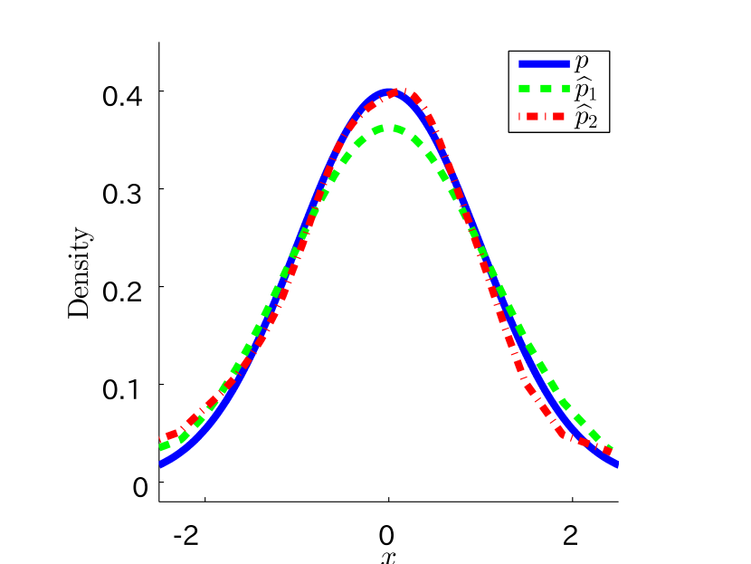
(a) Density estimation

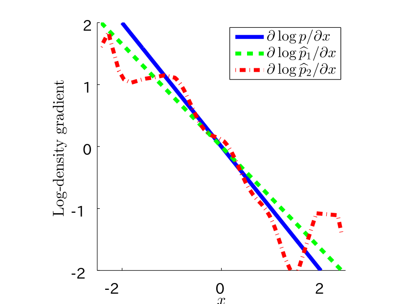
(b) Log-density gradient estimation

Figure 1: A comparison of two log-density gradient estimates based on density estimation. In (a), $\widehat{p}_{2}$ is a better estimate to the true density $p$ than $\widehat{p}_{1}$, while in (b), $\nabla\log\widehat{p}_{1}$ is a better estimate to the true log-density gradient $\nabla\log p$ than $\nabla\log\widehat{p}_{2}$.

Suppose that we are given a set of samples, $\{\bm{x}_{i}\}_{i=1}^{n}$, which are independent and identically distributed from a probability distribution with unknown density $p(\bm{x})$ on $\mathbb{R}^{d}$. The problem is to estimate the gradient of the logarithm of the density $p(\bm{x})$ from $\{\bm{x}_{i}\}_{i=1}^{n}$:

$$\nabla\log p(\bm{x}) =\left(\partial_{1}\log p(\bm{x}),\dotsc,\partial_{d}\log p(\bm{x})\right)^{\top}=\left(\frac{\partial_{1}p(\bm{x})}{p(\bm{x})},\dotsc,\frac{\partial_{d}p(\bm{x})}{p(\bm{x})}\right)^{\top},$$

where $\partial_{j}$ denotes the partial derivative operator $\partial/\partial x^{(j)}$ for $\bm{x}=(x^{(1)},\dots,x^{(d)})^{\top}$.

A naive method for estimating the log-density gradient is to first estimate the probability density, which is performed by, e.g., kernel density estimation (KDE) as

$$\widehat{p}(\bm{x})=\frac{1}{n}\sum_{i=1}^{n}\frac{1}{\left(2\pi\sigma^{2}\right)^{\frac{d}{2}}}\exp\left(-\frac{\|\bm{x}-\bm{x}_{i}\|^{2}}{2\sigma^{2}}\right),$$

where $\sigma>0$ denotes the Gaussian bandwidth, then to take the gradient of the logarithm of $\widehat{p}(\bm{x})$ as

$$\partial_{j}\log\widehat{p}(\bm{x})=\frac{\partial_{j}\widehat{p}(\bm{x})}{\widehat{p}(\bm{x})}.$$

However, this two-step method does not work well because an accurate density estimate does not necessarily provide an accurate log-density gradient estimate. For example, Figure 1 illustrates that a worse (or better) density estimate can produce a better (or worse) gradient estimate.

To overcome this problem, LSLDG, a single-step method which directly estimates the gradient without going through density estimation, was proposed (Beran, 1976; Cox, 1985; Sasaki et al., 2014), and has been demonstrated to experimentally work well. Next, we review LSLDG.

2.2 Direct estimation of log-density gradients

The basic idea of LSLDG is to directly fit a model $g_{j}(\bm{x})$ to the true log-density gradient $\partial_{j}\log p(\bm{x})$ under the squared loss:

$$R_{j}(g_{j}) :=\int\left(g_{j}(\bm{x})-\partial_{j}\log p(\bm{x})\right)^{2}p(\bm{x})\text{d}\bm{x}$$

$$\phantom{:}=\int\left(g_{j}(\bm{x})-\frac{\partial_{j}p(\bm{x})}{p(\bm{x})}\right)^{2}p(\bm{x})\text{d}\bm{x}$$

$$\phantom{:}=\int g_{j}(\bm{x})^{2}p(\bm{x})\text{d}\bm{x}-2\int g_{j}(\bm{x})\partial_{j}p(\bm{x})\text{d}\bm{x}+C_{j}$$

$$\phantom{:}=\int g_{j}(\bm{x})^{2}p(\bm{x})\text{d}\bm{x}-2\int\big{[}g_{j}(\bm{x})p(\bm{x})\big{]}_{x^{(j)}=-\infty}^{x^{(j)}=\infty}\text{d}\bm{x}^{(\setminus j)}+2\int\partial_{j}g_{j}(\bm{x})p(\bm{x})\text{d}\bm{x}+C_{j}$$

$$\phantom{:}=\int g_{j}(\bm{x})^{2}p(\bm{x})\text{d}\bm{x}+2\int\partial_{j}g_{j}(\bm{x})p(\bm{x})\text{d}\bm{x}+C_{j},$$

where $C_{j}:=\int\left(\partial_{j}p(\bm{x})\right)^{2}p(\bm{x})\text{d}\bm{x}$ is a constant that does not depend on $g_{j}$, $\int(\cdot)\text{d}\bm{x}^{({\setminus j})}$ denotes integration except for $x^{(j)}$, and the last deformation comes from integration by parts under the mild condition that $g_{j}(\bm{x})p(\bm{x})\to 0$ as $|x^{(j)}|\rightarrow\infty$.

Then, the LSLDG score $J_{j}(g_{j})$ is given as an empirical approximation to the risk $R_{j}(g_{j})$ subtracted by $C_{j}$:

$$J_{j}(g_{j}):=\frac{1}{n}\sum_{i=1}^{n}g_{j}(\bm{x}_{i})^{2}+\frac{2}{n}\sum_{i=1}^{n}\partial_{j}g_{j}(\bm{x}_{i}).$$ (1)

As $g_{j}(\bm{x})$, a linear-in-parameter model is used:

$$g_{j}(\bm{x})=\bm{\theta}_{j}^{\top}\bm{\psi}_{j}(\bm{x})=\sum_{k=1}^{b}\theta_{j}^{(k)}\psi_{j}^{(k)}(\bm{x}),$$ (2)

where $\theta_{j}^{(k)}$ is a parameter, $\psi_{j}^{(k)}(\bm{x})$ is a differentiable basis function, and $b$ is the number of the basis functions. By substituting (2) into (1) and adding an $\ell_{2}$-regularizer, we can analytically obtain the optimal solution $\widehat{\bm{\theta}}_{j}$ as

$$\widehat{\bm{\theta}}_{j} =\arg\min_{\bm{\theta}_{j}}\left[\bm{\theta}_{j}^{\top}\bm{G}_{j}\bm{\theta}_{j}+2\bm{h}_{j}^{\top}\bm{\theta}_{j}+\lambda_{j}\|\bm{\theta}_{j}\|^{2}\right]$$

$$=-(\bm{G}_{j}+\lambda_{j}\bm{I}_{b})^{-1}\bm{h}_{j},$$

where $\lambda_{j}\geq 0$ is the regularization parameter, $\bm{I}_{b}$ is the $b\times b$ identity matrix, and

$$\bm{G}_{j}:=\frac{1}{n}\sum_{i=1}^{n}\bm{\psi}_{j}(\bm{x}_{i})\bm{\psi}_{j}(\bm{x}_{i})^{\top},\ \bm{h}_{j}:=\frac{1}{n}\sum_{i=1}^{n}\partial_{j}\bm{\psi}_{j}(\bm{x}_{i}).$$

Finally, an estimator of the log-density gradient is obtained by

$$\hat{g}_{j}(\bm{x}):=\hat{\bm{\theta}}_{j}^{\top}\bm{\psi}_{j}(\bm{x}).$$

It was experimentally shown that LSLDG produces much more accurate estimates of log-density gradients than the KDE-based gradient estimator and that the clustering method based on LSLDG performs well (Sasaki et al., 2014).

3 Regularized multi-task learning

In this section, we review a multi-task learning framework called regularized multi-task learning (Evgeniou and Pontil, 2004; Evgeniou et al., 2005), which is powerful and widely applicable to many machine learning methods.

Consider that we have $T$ tasks of supervised learning as follows. The task $t$ is to learn an unknown function $f_{t}^{*}(\bm{x})$ from samples of input-output pairs $\{(\bm{x}_{i}^{(t)},y_{i}^{(t)})\}_{i=1}^{n_{t}}$, where $y_{i}^{(t)}$ is the output $f_{t}^{*}(\bm{x})$ with noise at the input $\bm{x}=\bm{x}_{i}^{(t)}$. When $f_{t}^{*}(\bm{x})$ is modeled by a parameterized function $f_{t}(\bm{x};\bm{\theta}_{t})$, learning is performed by finding the parameter $\bm{\theta}_{t}$ which minimizes the empirical risk associated with some loss function $l(y,y^{\prime})$:

$$\widehat{\bm{\theta}}_{t} =\arg\min_{\bm{\theta}_{t}}\frac{1}{n_{t}}\sum_{i=1}^{n_{t}}l(y_{i}^{(t)},f_{t}(\bm{x}_{t}^{(t)};\bm{\theta}_{t}))=\arg\min_{\bm{\theta}_{t}}J_{t}(\bm{\theta}_{t}),$$

where $J_{t}(\bm{\theta}_{t})=\sum_{i=1}^{n_{t}}l(y_{i}^{(t)},f_{t}(\bm{x}_{t}^{(t)};\bm{\theta}_{t}))$.

In regularized multi-task learning, the objective function has regularization terms which impose every pair of parameters to be close to each other while $J_{t}(\bm{\theta}_{t})$ are jointly minimized:

$$\sum_{t=1}^{T}J_{t}(\bm{\theta}_{t})+\frac{1}{2}\gamma\sum_{t=1,t^{\prime}=1}^{T}\gamma_{t,t^{\prime}}\|\bm{\theta}_{t}-\bm{\theta}_{t^{\prime}}\|^{2},$$

where $\gamma\geq 0$ is the regularization parameter and $\gamma_{t,t^{\prime}}\geq 0$ are the similarity parameters between the tasks $t$ and $t^{\prime}$.

It was experimentally demonstrated that the multi-task support vector regression (Evgeniou and Pontil, 2004; Evgeniou et al., 2005), performs better than the single-task counterpart (Vapnik et al., 1997) especially when the tasks are highly related each other.

4 Proposed method

In this section, we present our proposed method and algorithms.

4.1 Basic idea

Our goal in this paper is to improve the performance of LSLDG in multi-dimensional cases. For multi-dimensional input $\bm{x}$, the log-density gradient $\nabla\log p(\bm{x})$ has multiple output dimensions, meaning that its estimation actually consists of multiple learning tasks. Our basic idea is to apply regularized multi-task learning to solve these tasks simultaneously instead of learning them independently.

This idea is supported by the fact that the target functions of these tasks, $\partial_{1}\log p(\bm{x}),\dots,\partial_{d}\log p(\bm{x})$, are all derived from the same log-density $\log p(\bm{x})$, and thus they must be strongly related to each other. Under such strong relatedness, jointly learning them with sharing information with each other would improve estimation accuracy as has been observed in other existing multi-task learning work.

4.2 Regularized multi-task learning for least-squares log-density gradients (MT-LSLDG)

Here, we propose a method called regularized multi-task learning for least-squares log-density gradients (MT-LSLDG).

Our method MT-LSLDG is given by applying regularized multi-task learning to LSLDG. Specifically, we consider the problem of minimizing the following objective function:

$$J(\bm{\theta}_{1},\dots,\bm{\theta}_{d}) =\sum_{j=1}^{d}J_{j}(g_{j}(\cdot;\bm{\theta}_{j}))+\sum_{j=1}^{d}\lambda_{j}\|\bm{\theta}_{j}\|^{2}+\frac{1}{2}\gamma\sum_{j,j^{\prime}=1}^{d}\gamma_{j,j^{\prime}}\|\bm{\theta}_{j}-\bm{\theta}_{j^{\prime}}\|^{2}$$

$$=\sum_{j=1}^{d}\left(\bm{\theta}_{j}^{\top}\bm{G}_{j}\bm{\theta}_{j}+2\bm{\theta}_{j}^{\top}\bm{h}_{j}+\lambda_{j}\|\bm{\theta}_{j}\|^{2}\right)+\frac{1}{2}\gamma\sum_{j,j^{\prime}=1}^{d}\gamma_{j,j^{\prime}}\|\bm{\theta}_{j}-\bm{\theta}_{j^{\prime}}\|^{2},$$ (3)

where the last term is the multi-task regularizer which imposes the parameters close to each other.

Denoting the minimizers of (3) by $\bm{\widehat{\theta}}_{1},\dots,\bm{\widehat{\theta}}_{d}$, the estimator $\widehat{\bm{g}}(\bm{x})=(\widehat{g}_{1}(\bm{x}),\dots,\widehat{g}_{d}(\bm{x}))^{\top}$ is given by

$$\widehat{g}_{j}(\bm{x})=g_{j}(\bm{x};\widehat{\bm{\theta}}_{j})=\widehat{\bm{\theta}}_{j}^{\top}\bm{\psi}_{j}(\bm{x}).$$ (4)

We call this method regularized multi-task learning for least-squares log-density gradients (MT-LSLDG).

4.3 The design of the basis functions

The design of the basis functions $\bm{\psi}_{j}(\bm{x})$ in MT-LSLDG is crucial to enjoy the advantage of regularized multi-task learning. A simple design would be to use a common function $\bm{\phi}(\bm{x})=(\phi^{(1)}(\bm{x}),\dots,\phi^{(b)}(\bm{x}))$ to all $\bm{\psi}_{j}(\bm{x})$, that is, $\bm{\psi}_{1}(\bm{x})=\dots=\bm{\psi}_{d}(\bm{x})=\bm{\phi}(\bm{x})$. From (3) and (4), in this design, the multi-task regularizer promotes $\widehat{g}_{j}(\bm{x};\widehat{\bm{\theta}}_{j})$ to be more close to each other so that

$$\widehat{g}_{1}(\bm{x};\widehat{\bm{\theta}}_{1})\approx\dots\approx\widehat{g}_{d}(\bm{x};\widehat{\bm{\theta}}_{d}).$$

However, it is inappropriate that all $\widehat{g}_{j}(\bm{x};\widehat{\bm{\theta}}_{j})$ are similar because the different true partial derivatives, say $\partial_{j}\log p(\bm{x})$ and $\partial_{j^{\prime}}\log p(\bm{x})$ for $j\neq j^{\prime}$, show different profiles in general.

To avoid this problem, we propose to use the partial derivatives of $\bm{\phi}(\bm{x})$ as basis functions:

$$\bm{\psi}_{j}^{(k)}(\bm{x})=\partial_{j}\bm{\phi}(\bm{x}).$$

For this basis function design, it holds that

$$\widehat{\bm{g}}_{j}(\bm{x})=\widehat{\bm{\theta}}_{j}^{\top}\bm{\psi}_{j}(\bm{x})=\widehat{\bm{\theta}}_{j}^{\top}\partial_{j}\bm{\phi}(\bm{x})=\partial_{j}\widehat{\bm{\theta}}_{j}^{\top}\bm{\phi}(\bm{x})\approx\partial_{j}\log p(\bm{x}).$$

Thus, $\widehat{\bm{\theta}}_{j}^{\top}\bm{\phi}(\bm{x})$ are approximations of the true log-density $\log p(\bm{x})$. Since the multi-task regularizer encourages the log-density estimates $\widehat{\bm{\theta}}_{j}^{\top}\bm{\phi}(\bm{x})$ to be more similar, this basis design would be reasonable.

As a specific choice of $\phi^{(k)}(\bm{x})$, we use a Gaussian kernel:

$$\psi_{j}^{(k)}(\bm{x}) =\partial_{j}\exp\left(-\frac{\|\bm{x}-\bm{c}_{k}\|^{2}}{2\sigma_{j}^{2}}\right)$$

$$=\frac{c_{k}^{(j)}-x^{(j)}}{\sigma_{j}^{2}}\exp\left(-\frac{\|\bm{x}-\bm{c}_{k}\|^{2}}{2\sigma_{j}^{2}}\right),$$

where $\bm{c}_{k}$ are the centers of the kernels, and $\sigma_{j}>0$ are the Gaussian band width parameters.

4.4 Hyper-parameter selection by cross-validation

As in LSLDG, the hyper parameters, which are the $\ell_{2}$-regularization parameters $\lambda_{j}$, the Gaussian width $\sigma_{j}$, and the multi-task parameters $\gamma,\gamma_{j,j^{\prime}}$, can be cross-validated in MT-LSLDG. The procedure of the $K$-fold cross-validation is as follows: First, we randomly partition the set of training samples $S_{\text{tr}}$ into $K$ folds $F_{1},\dots,F_{K}$. Next, for each $k=1,\dots,K$, we estimate the log-density gradient using the samples in $S_{\text{tr}}\setminus F_{k}$ , which is denoted by $\hat{g}_{j}^{(k)}$, and then calculate the LSLDG scores for the samples in $F_{k}$ as $J_{\text{CV}}^{(k)}$:

$$J_{\text{CV}}^{(k)}=\frac{1}{|F_{k}|}\sum_{\bm{x}\in F_{k}}\widehat{g}_{j}^{(k)}(\bm{x})^{2}+\frac{2}{|F_{k}|}\sum_{\bm{x}\in F_{k}}\frac{\partial\widehat{g}_{j}^{(k)}(\bm{x})}{\partial x^{(j)}}.$$

We average these LSLDG scores to obtain the $K$-fold cross-validated LSLDG score:

$$J_{\text{CV}}=\frac{1}{K}\sum_{k=1}^{K}J_{\text{CV}}^{(k)}.$$

Finally, we choose the hyper-parameters that minimize $J_{\text{CV}}$. Throughout this paper, we set $K=5$.

4.5 Optimization algorithms in MT-LSLDG

Here, we develop two algorithms for minimizing (3). One algorithm is to directly evaluate the analytic solution and the other is an iterative method based on block coordinate descent (Warga, 1963).

4.5.1 Analytic solution

For simplicity, we assume the similarity parameters are symmetric: $\gamma_{j,j^{\prime}}=\gamma_{j^{\prime},j}$. Then, the objective function $J(\bm{\theta}_{1},\dots,\bm{\theta}_{d})$ can be expressed as a quadratic function in terms of $\bm{\theta}=(\bm{\theta}_{1}^{\top},\dots,\bm{\theta}_{d}^{\top})^{\top}$ as

$$J(\bm{\theta}) =\bm{\theta}^{\top}(\bm{G}+\bm{C}\otimes\bm{I}_{b})\bm{\theta}+2\bm{\theta}^{\top}\bm{h},$$

where

$$\bm{G} =\operatorname{diag}(\bm{G}_{1},\dots,\bm{G}_{d}),\ \bm{h}=(\bm{h}_{1}^{\top},\dots,\bm{h}_{d}^{\top})^{\top},$$

$$\bm{C} :=\operatorname{diag}(\lambda_{1},\dots,\lambda_{d})+\gamma\operatorname{diag}\left(\sum_{j=1}^{d}\gamma_{1,j},\dots,\sum_{j=1}^{d}\gamma_{d,j}\right)-\gamma\bm{\Gamma},$$

$[\bm{\Gamma}]_{j,j^{\prime}}=\gamma_{j,j^{\prime}}$, $\operatorname{diag}(\cdot,\dots,\cdot)$ is a block-diagonal matrix whose diagonal blocks are its arguments, and $\otimes$ denotes the Kronecker product. The minimizer $\widehat{\bm{\theta}}$ of $J(\bm{\theta})$ is analytically computed by

$$\widehat{\bm{\theta}} =\arg\min_{\bm{\theta}}J(\bm{\theta})=-(\bm{G}+\bm{C}\otimes\bm{I}_{b})^{-1}\bm{h}.$$ (5)

4.5.2 Block coordinate descent (BCD) method

Direct computation of the analytic solution (5) involves inversion of a $db\times db$ matrix. This may be not only expensive in terms of computation time but also infeasible in terms of memory space when the dimensionality $d$ is very large.

Alternatively, we propose an algorithm based on block coordinate descent (BCD) (Warga, 1963). It is an iterative algorithm which only needs manipulation of a relatively small $b\times b$ matrix at each iteration. This alleviates the memory size requirement and hopefully reduces computation time if the number of iterations is not large.

A pseudo code of the algorithm is shown in Algorithm 1. At each update (6) in the algorithm, only one vector $\widehat{\bm{\theta}}_{j}$ is optimized in a closed-form while fixing the other parameters $\widehat{\bm{\theta}}_{j^{\prime}}$ ($j^{\prime}\neq j$). The update (6) only requires computing the inverse of a $b\times b$ matrix, which seems to be computationally advantageous over evaluating the analytic solution in terms of the computation cost and memory size requirement.

Another important technique to reduce the overall computation time is to use warm start initialization: when the optimal value of $\gamma$ is searched for by cross-validation, we may use the solutions $\widetilde{\bm{\theta}}_{1},\dots,\widetilde{\bm{\theta}}_{d}$ obtained with $\gamma$ as initial values for another $\gamma$.

Algorithm 1 Block coordinate descent (BCD) algorithm.

Initialize $\widetilde{\bm{\theta}}_{1},\dots,\widetilde{\bm{\theta}}_{d}$.

repeat

     for $j=1,\dots,d$ do

         

$$\widetilde{\bm{\theta}}_{j} \leftarrow\arg\min_{\bm{\theta}_{j}}J(\widetilde{\bm{\theta}}_{1},\dotsc,\widetilde{\bm{\theta}}_{j-1},\bm{\theta}_{j},\widetilde{\bm{\theta}}_{j+1},\dotsc,\widetilde{\bm{\theta}}_{d})$$

$$=\left(\bm{G}_{j}+\lambda_{j}\bm{I}_{b}+2\gamma\sum_{j\neq j^{\prime}}\gamma_{j,j^{\prime}}\bm{I}_{b}\right)^{-1}\left(-\bm{h}_{j}+2\gamma\sum_{j^{\prime}\neq j}\gamma_{j,j^{\prime}}\widetilde{\bm{\theta}}_{j^{\prime}}\right).$$ (6)

     end for

until $\widetilde{\bm{\theta}}_{1},\dots,\widetilde{\bm{\theta}}_{d}$ converge.

5 Experiments on log-density gradient estimation

In this section, we illustrate the behavior of the proposed method and experimentally investigate its performance.

5.1 Experimental setting

In each experiment, training samples $\{\bm{x}_{i}\}_{i=1}^{n}$ and test samples $\{\bm{x}^{\prime}_{i^{\prime}}\}_{i^{\prime}=1}^{n^{\prime}}$ are drawn independently from an unknown density $p(\bm{x})$. We estimate $\nabla\log p(\bm{x})$ from the training samples, and then evaluate the estimation performance by the test score

$$J_{\text{te}}(\widehat{\bm{g}})=\sum_{j=1}^{d}\left[\frac{1}{n^{\prime}}\sum_{i^{\prime}=1}^{n^{\prime}}\widehat{g}_{j}(\bm{x}^{\prime}_{i^{\prime}})^{2}+\frac{2}{n^{\prime}}\sum_{i^{\prime}=1}^{n^{\prime}}\partial_{j}\widehat{g}_{j}(\bm{x}^{\prime}_{i^{\prime}})\right],$$

where $\widehat{\bm{g}}(\bm{x})=(\widehat{g}_{1}(\bm{x}),\dots,\widehat{g}_{d}(\bm{x}))^{\top}$ is an estimated log-density gradient. This score is an empirical approximation of the expected squared loss of $\widehat{\bm{g}}(\bm{x})$ over the test samples without the constant $C_{j}$ (see Section 2.2), and a smaller score means a better estimate.

We compare the following three methods:

• The multi-task LSLDG (MT-LSLDG): our method proposed in Section 4.

• The single-task LSLDG (S-LSLDG): the existing method (Beran, 1976; Cox, 1985) reviewed in Section 2.2. This method agrees with MT-LSLDG at $\gamma=0$.

• The common-parameter LSLDG (C-LSLDG): LSLDG with common parameters $\bm{\theta}^{\prime}=\bm{\theta}_{1}=\dots=\bm{\theta}_{d}$ learned simultaneously. The solution is given as

  $$\widehat{\bm{\theta}^{\prime}} =\arg\min_{\bm{\theta}^{\prime}}\left[\bm{\theta}^{\prime\top}\sum_{j=1}^{d}\bm{G}_{j}\bm{\theta}^{\prime}+2\sum_{j=1}^{d}\bm{h}_{j}^{\top}\bm{\theta}^{\prime}+\lambda\|\bm{\theta}^{\prime}\|^{2}\right]$$

  $$=-\left(\sum_{j=1}^{d}\bm{G}_{j}+\lambda\bm{I}_{b}\right)^{-1}\sum_{j=1}^{d}\bm{h}_{j},$$

  where $\lambda\geq 0$ is the $\ell_{2}$-regularization parameter. This method agrees with MT-LSLDG at the limit $\gamma\to\infty$.

In all the methods, we set the number of basis functions as $b=\min\{50,n\}$, and randomly choose the kernel centers $\bm{c}_{1},\dots,\bm{c}_{b}$ from training samples $\{\bm{x}_{i}\}_{i=1}^{n}$. For hyper-parameters, we use the common $\ell_{2}$-regularization parameter $\lambda$ and bandwidth parameter $\sigma$ among all the dimensions, $\lambda_{1}=\dots=\lambda_{d}=\lambda$ and $\sigma_{1}=\dots=\sigma_{d}=\sigma$. We also set all the similarity parameters as $\gamma_{j,j^{\prime}}=1$, which assumes that all dimensions are equally related to each other.

5.2 Artificial data

We conduct numerical experiments on artificial data to investigate the basic behavior of MT-LSLDG. As data density $p(\bm{x})$, we consider the following two cases:

• Single Gaussian: The $d$-dimensional Gaussian density whose mean is $\bm{0}$ and whose covariance matrix is the diagonal matrix with the first half of the diagonal elements are $1$ and the others are $5$.

• Double Gaussian: A mixture of two $d$-dimensional Gaussian densities with mean zero and $(5,0,\dots,0)^{\top}$ and identity covariance matrix. The mixing coefficients are $1/2$.

The dimensionality $d$ and sample size $n$ are specified later.

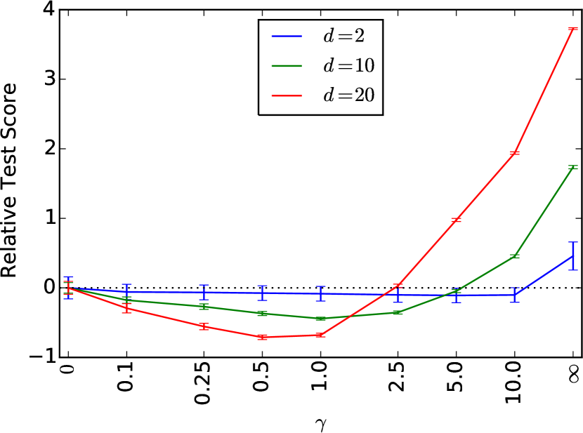
(a) Single Gaussian ($n=30$)

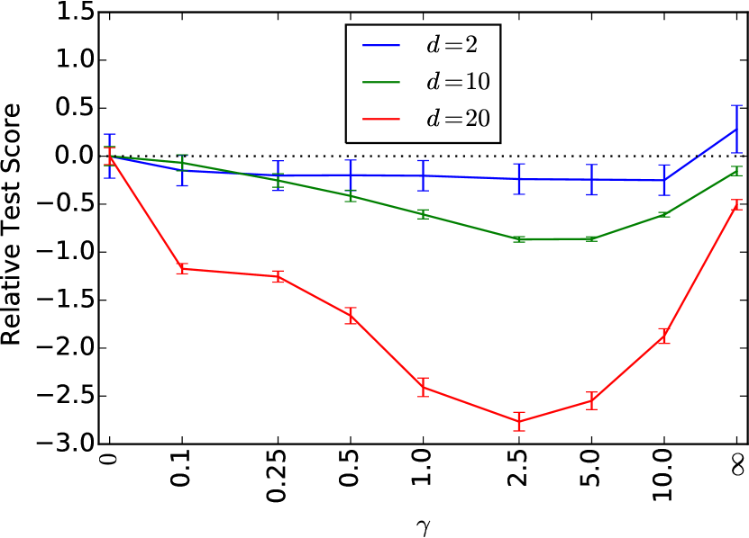
(b) Double Gaussian ($n=30$)

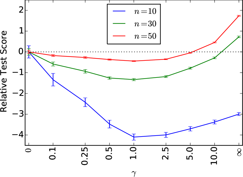
(c) Single Gaussian ($d=10$)

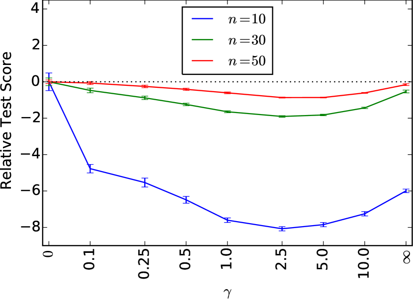
(d) Double Gaussian ($d=10$)

Figure 2: Average (and standard errors) of relative test scores over 100 runs. The relative test scores refer to test scores from which the test score of S-LSLDG is subtracted. The black dotted lines indicate the relative score zero.

First, we investigate whether MT-LSLDG improves the estimation accuracy of LSLDG at appropriate $\gamma$. We prepare datasets with different dimensionalities $d=2,10,20$ and sample sizes $n=10,30,50$. MT-LSLDG is applied to the datasets at each $\gamma\in\{0,0.1,0.25,0.5,1,2.5,5,10,\infty\}$. The Gaussian bandwidth $\sigma$ and the $\ell_{2}$-regularization parameter $\lambda$ are chosen by $5$-fold cross-validation as described in Section 4 from the candidate lists $\{10^{-1},10^{-0.25},10^{0.5},10^{1.25},10^{2}\}$ and $\{10^{-2},10^{-1.25},10^{0.5},10^{0.25},10^{1}\}$, respectively. The solution of MT-LSLDG is computed analytically as in (5).

The results are plotted in Figure 2. In the figure, the relative test score is defined as the test score from which the test score of S-LSLDG is subtracted, and thus negative relative scores indicate that MT-LSLDG improved the performance of S-LSLDG. When $d=2$, MT-LSLDG does not improve the performance for any $\gamma$ values (Figure 2(a) and 2(b)). However, for higher-dimensional data, the performance is improved at appropriate $\gamma$ values (e.g., $\gamma=0.5$ for $d=20$ in Figure 2(a) and $\gamma=2.5$ for $d=20$ in Figure 2(b)). Similar improvement is observed also for smaller sample size (e.g., $n=10$ and $n=30$) in Figure 2(c) and Figure 2(d).

These results confirm that MT-LSLDG improves the performance of S-LSLDG at an appropriate $\gamma$ value when data is relatively high-dimensional and the sample size is small. Since such $\gamma$ is usually unknown in advance, we need to find a reasonable value in practice.

Next, we investigate whether an appropriate $\gamma$ value can be chosen by cross-validation. In this experiment, the cross-validation method in Section 4.4 is performed to choose $\gamma$ as well. The candidates of $\gamma$ is $\{0,0.1,0.25,0.5,1,2.5,5,10,\infty\}$. The other experimental settings such as the data generation and all the LSLDGs are the same as in the last experiment.

Table 1 shows that MT-LSLDG improves the performance especially when the dimensionality of data is relatively high and the sample size is small. These results indicate that the proposed cross-validation method allows us to choose a reasonable $\gamma$ value.

Table 1: Averages (and standard errors) of test scores on the artificial data with cross-validation over 100 runs. In each row, the best and comparable to the best scores in terms of paired t-test with significance level $5\%$ are emphasized in bold face.

Density	$n$	MT-LSLDG	S-LSLDG	C-LSLDG
Single Gaussian	$10$	$\bm{-2.87}$ ($0.22$)	$0.37$ ($0.31$)	$\bm{-2.58}$ ($0.07$)
	$30$	$\bm{-5.34}$ ($0.038$)	$-4.97$ ($0.08$)	$-3.29$ ($0.03$)
	$50$	$\bm{-5.63}$ ($0.02$)	$-5.55$ ($0.02$)	$-4.13$ ($0.04$)
Double Gaussian	$10$	$\bm{-6.83}$ ($0.14$)	$1.01$ ($0.54$)	$-5.02$ ($0.12$)
	$30$	$\bm{-8.45}$ ($0.03$)	$-7.63$ ($0.10$)	$-7.84$ ($0.04$)
	$50$	$\bm{-8.67}$ ($0.02$)	$-8.29$ ($0.10$)	$-8.48$ ($0.02$)

Density	$d$	MT-LSLDG	S-LSLDG	C-LSLDG
Single Gaussian	$2$	$\bm{0.20}$ ($0.19$)	$\bm{-0.11}$ ($0.15$)	$\bm{0.09}$ ($0.15$)
	$10$	$\bm{-5.34}$ ($0.04$)	$-4.97$ ($0.08$)	$-3.29$ ($0.03$)
	$20$	$\bm{-10.77}$ ($0.03$)	$-9.98$ ($0.13$)	$-6.39$ ($0.01$)
Double Gaussian	$2$	$\bm{0.54}$ ($0.22$)	$\bm{0.50}$ ($0.27$)	$\bm{0.19}$ ($0.22$)
	$10$	$\bm{-8.45}$ ($0.03$)	$-7.63$ ($0.10$)	$-7.84$ ($0.04$)
	$20$	$\bm{-16.9}$ ($0.14$)	$-14.90$ ($0.10$)	$-15.26$ ($0.06$)

5.3 Benchmark data

In this section, we demonstrate the usefulness of MT-LSLDG in gradient estimation on various benchmark datasets.

This experiment uses IDA benchmark repository (Rätsch et al., 2001). For MT-LSLDG, the hyper-parameters $\sigma$, $\lambda$ and $\gamma$ are chosen by cross-validation. The candidate lists are $\sigma\in\{0.1,0.25,0.5,1,2.5,5,10\}$, $\lambda\in\{10^{-5},10^{-4},\dots,10^{-1}\}$ and $\gamma\in\{0,10^{-5},10^{-4},\dots,10^{1},10^{2},\infty\}$, respectively. For S-LSLDG and C-LSLDG, the candidate lists of $\sigma$ and $\lambda$ are the same as MT-LSLDG. The solution of MT-LSLDG is computed by the BCD algorithm described in Section 4.5.2.

The results are presented in Table 2. MT-LSLDG significantly improves the performance of either S-LSLDG or C-LSLDG on most of the datasets.

Table 2: Avarages (and standard errors) of the test scores on IDA datasets. In each dataset, the best and comparable to the best scores in terms of paired t-test with significance level $5\%$ are emphasized in bold face. The number of trials is 20 for the image and splice dataset, and is 100 for the other datasets.

Dataset ($d$, $n$)	MT-LSLDG	S-LSLDG	C-LSLDG
thyroid ($5$, $140$)	$\bm{-111}$ ($7$)	$\bm{-103}$ ($8$)	$-40$ ($4$)
diabetes ($8$, $468$)	$\bm{-21.2}$ ($3.9$)	$\bm{-18.0}$ ($4.5$)	$\bm{-15.1}$ ($0.1$)
flare-solar ($9$, $666$)	$\bm{-1.4\times 10^{7}}$ ($0.0\times 10^{7}$)	$-0.2\times 10^{7}$ ($0.0\times 10^{7}$)	$-1.4\times 10^{7}$ ($0.0\times 10^{7}$)
breast-cancer ($9$, $200$)	$\bm{-2.6\times 10^{3}}$ ($0.2\times 10^{3}$)	$-0.2\times 10^{3}$ ($0.0\times 10^{3}$)	$\bm{-2.6\times 10^{3}}$ ($0.2\times 10^{3}$)
image ($18$, $1300$)	$\bm{-2.0\times 10^{4}}$ ($0.0\times 10^{4}$)	$\bm{-2.0\times 10^{4}}$ ($0.0\times 10^{4}$)	$-0.0\times 10^{4}$ ($0.0\times 10^{4}$)
german ($20$, $700$)	$\bm{-3.1\times 10^{2}}$ ($0.1\times 10^{2}$)	$\bm{-3.0\times 10^{2}}$ ($0.1\times 10^{2}$)	$-0.2\times 10^{2}$ ($0.0\times 10^{2}$)
twonorm ($20$, $400$)	$\bm{-22.3}$ ($0.0$)	$\bm{-22.3}$ ($0.0$)	$-22.1$ ($0.0$)
waveform ($21$, $400$)	$\bm{-43}$ ($0$)	$-43$ ($0$)	$-35$ ($0$)
splice ($60$, $1000$)	$\bm{-1.8\times 10^{3}}$ ($0.6\times 10^{3}$)	$-0.0\times 10^{3}$ ($0.0\times 10^{3}$)	$\bm{-2.0\times 10^{3}}$ ($0.6\times 10^{3}$)

6 Application to mode-seeking clustering

In this section, we apply MT-LSLDG to mode-seeking clustering and experimentally demonstrate its usefulness.

6.1 Mode-seeking clustering

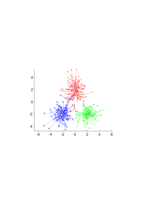
Figure 3: Transition of data points during a mode-seeking process. Data samples are drawn from a mixture of Gaussians, and the data points sampled from the same Gaussian component are specified by the same color (red, green, or blue) and marker (plus symbol, circle, or triangle). White squares indicate the points to which data points converged.

A practical application of log-density gradient estimation is mode-seeking clustering (Fukunaga and Hostetler, 1975; Cheng, 1995; Comaniciu and Meer, 2002; Sasaki et al., 2014). Mode-seeking clustering methods update each data point toward a nearby mode by gradient ascent, and assign the same clustering label to the data points which converged to the same mode (Figure 3). Their notable advantage is that we need not specify the number of clusters in advance. Mode-seeking clustering has been successfully applied to a variety of real world problems such as object tracking (Comaniciu et al., 2000), image segmentation (Comaniciu and Meer, 2002; Sasaki et al., 2014), and line edge detection in images (Bandera et al., 2006).

In mode-seeking, the essential ingredient is the gradient of the data density. To estimate the gradients, mean shift clustering (Fukunaga and Hostetler, 1975; Cheng, 1995; Comaniciu and Meer, 2002), which is one of the most popular mode-seeking clustering methods, employs the two-step method of first estimating the data density by kernel density estimation and then taking its gradient. However, as we mentioned earlier, this two-step method does not work well since accurately estimating the density does not necessarily lead to an accurate estimate of the gradient.

In order to overcome this problem, LSLDG clustering (Sasaki et al., 2014) adopted LSLDG instead of the two-step method. Sasaki et al. (2014) also provided a practically useful fixed-point algorithm for mode-seeking as in mean shift clustering (Cheng, 1995): When the partial derivative of a vector of Gaussian kernels $\bm{\psi}_{j}(\bm{x})=\partial_{j}\bm{\phi}(\bm{x})$ is used as the vector of basis functions, the model $g_{j}(\bm{x})=\widehat{\bm{\theta}}_{j}^{\top}\bm{\psi}_{j}(\bm{x})$ can be transformed as

$$\widehat{g}_{j}(\bm{x}) =\sum_{k=1}^{b}\widehat{\theta}_{j}^{(k)}\frac{c_{k}^{(j)}-x^{(j)}}{\sigma^{2}}\phi^{(k)}(\bm{x})$$

$$=\frac{1}{\sigma^{2}}\sum_{k=1}^{b}\widehat{\theta}_{j}^{(k)}c_{k}^{(j)}\phi^{(k)}(\bm{x})-\frac{x^{(j)}}{\sigma^{2}}\sum_{k=1}^{b}\widehat{\theta}_{j}^{(k)}\phi^{(k)}(\bm{x})$$

$$=\left[\frac{1}{\sigma^{2}}\sum_{k=1}^{b}\widehat{\theta}_{j}^{(k)}\phi^{(k)}(\bm{x})\right]\left[\frac{\sum_{k^{\prime}=1}^{b}\widehat{\theta}_{j}^{(k^{\prime})}c_{k^{\prime}}^{(j)}\phi^{(k^{\prime})}(\bm{x})}{\sum_{k^{\prime}=1}^{b}\widehat{\theta}_{j}^{(k^{\prime})}\phi^{(k^{\prime})}(\bm{x})}-x^{(j)}\right],$$

where we assume that $\frac{1}{\sigma^{2}}\sum_{k=1}^{b}\widehat{\theta}_{j}^{(k)}\phi^{(k)}(\bm{x})$ is nonzero. Setting $\widehat{g}_{j}(\bm{x})$ to zero yields a fixed-point update formula as

$$x^{(j)}\leftarrow\frac{\sum_{k^{\prime}=1}^{b}\widehat{\theta}_{j}^{(k^{\prime})}c_{k^{\prime}}^{(j)}\phi^{(k^{\prime})}(\bm{x})}{\sum_{k^{\prime}=1}^{b}\widehat{\theta}_{j}^{(k^{\prime})}\phi^{(k^{\prime})}(\bm{x})}.$$

It has been experimentally shown that LSLDG clustering performs significantly better than mean-shift clustering (Sasaki et al., 2014).

Here, we apply MT-LSLDG to LSLDG clustering and investigate if the performance is improved in mode-seeking clustering as well for relatively high-dimensional data.

6.2 Experiments

Next, we conduct numerical experiments for mode-seeking clustering.

6.2.1 Experimental setting

We apply the following four clustering methods to various datasets:

• MT-LSLDGC: LSLDG clustering with MT-LSLDG.

• S-LSLDGC: LSLDG clustering with S-LSLDG (Sasaki et al., 2014).

• C-LSLDGC: LSLDG clustering with C-LSLDG (Sasaki et al., 2014).

• Mean-shift: mean shift clustering (Comaniciu and Meer, 2002).

For MTL-, S-, and C-LSLDG, all the hyper-parameters are cross-validated as described in Section 4.4, and for mean-shift, log-likelihood cross-validation is used.

We evaluate the clustering performance by the adjusted Rand index (ARI) (Hubert and Arabie, 1985). ARI gives one to the perfect clustering assignment and zero on average to a random clustering assignment. A larger ARI value means a better clustering result.

6.2.2 Artificial data

First, we conduct experiments on artificial data. The density of the artificial data is a mixture of three $d$-dimensional Gaussian densities with means $(0,2,0,\dots,0)$, $(-2,-2,0,\dots,0)$, and $(2,-2,0,\dots,0)$, covariance matrices $\tfrac{1}{\sqrt{2\pi}}\bm{I}_{d}$, and mixing coefficients $0.4$,$0.3$,$0.3$. The candidate lists of the hyper-parameters are the following: $\sigma\in\{10^{-1},10^{-7/9},10^{-5/9},\dots,10^{5/9},10^{7/9},10^{1}\}$, $\lambda\in\{10^{-5},10^{-4},10^{-3},10^{-2},10^{-1}\}$ and, $\gamma\in\{0,10^{-5},10^{-4},10^{-3},10^{-2},10^{-1},10^{0},10^{1},10^{2},\infty\}$.

The results are shown in Table 3. We can see that MT-LSLDGC performs well especially for the largest dimensionality $d=20$.

Table 3: Averages (and standard errors) of ARIs on real data. In each row, the best and comparable to the best ARI in terms of unpaired t-test with significance level $5\%$ is emphasized in bold face. The number of trials is 100.

$d$	MT-LSLDGC	S-LSLDGC	C-LSLDGC	Mean-shift
$2$	$\bm{0.992}$ ($0.035$)	$\bm{0.973}$ ($0.125$)	$\bm{0.992}$ ($0.036$)	$\bm{0.984}$ ($0.044$)
$10$	$\bm{0.993}$ ($0.004$)	$\bm{0.994}$ ($0.003$)	$\bm{0.994}$ ($0.004$)	$0.042$ ($0.022$)
$15$	$\bm{0.983}$ ($0.023$)	$\bm{0.982}$ ($0.054$)	$0.877$ ($0.217$)	$0.000$ ($0.000$)
$20$	$\bm{0.827}$ ($0.190$)	$0.586$ ($0.208$)	$0.716$ ($0.352$)	$0.036$ ($0.037$)

6.2.3 Real data

Next, we perform clustering on real data. The following three datasets are used:

• Accelerometry data: $5$-dimensional data used in (Hachiya et al., 2012) for human activity recognition extracted from mobile sensing data available from http://alkan.mns.kyutech.ac.jp/web/data. The number of classes is $3$. In each run of experiment, we use randomly chosen $100$ samples from each class. The total number of samples is $300$.

• Vowel data: $10$-dimensional data of recorded British English vowel sounds available from https://archive.ics.uci.edu/ml/datasets/Connectionist+Bench+(Vowel+Recognition+-+Deterding+Data). The number of classes is $11$ In each run of experiment, we use randomly chosen $500$.

• Sat-image data: $36$-dimensional multi-spectral satellite image available from https://archive.ics.uci.edu/ml/datasets/Statlog+(Landsat+Satellite). The number of classes is $6$. In each run of experiment, we use randomly chosen $2000$ samples.

• Speech data: $50$-dimensional voice data by two French speakers (Sugiyama et al., 2014). The number of classes is $2$. In each run of experiment, we use randomly chosen $200$ samples from each class. The total number of samples is $400$.

For MT-LSLDG, the hyper-parameters are cross-validated using the candidates, $\sigma\in\{10^{-1},10^{-6/9},10^{-3/9},\dots,10^{12/9},10^{15/9},10^{2}\}$, $\lambda\in\{10^{-5},10^{-4},10^{-3},10^{-2},10^{-1},10^{0}\}$ and $\gamma\in\{10^{-5},10^{-4},\dots,10^{1},10^{2}\}$, except that we use relatively small candidate lists $\sigma\in\{0.5,1,2.5,5,10\}$, $\lambda\in\{0.003,0.01,0.1,1\}$ and $\gamma\in\{0.1,1,10\}$ for the speech data since it has large dimensionality and optimization is computationally expensive. For S- and C-LSLDG, we used the same candidates of MT-LSLDG for $\sigma$ and $\lambda$. For mean shift clustering, the Gaussian kernel is employed in KDE, and the bandwidth parameter in the kernel is selected by 5-fold cross-validation with respect to the log-likelihood of the density estimate from the same candidates of MT-LSLDG for $\sigma$.

The results are shown in Table 4. For the accelerometry data whose dimensionality is only five, S-LSLDGC gives the best performance and MT-LSLDGC does not improve the performance, although MT-LSLDGC performs better than C-LSLDGC.

On the other hand, for the higher-dimensional dataset, the vowel data, the sat-image data, and the speech data, the performance of MT-LSLDGC is the best or comparable to the best. These results indicate that MT-LSLDG is a promising method in mode-seeking clustering especially when the dimensionality of data is relatively large.

Table 4: Averages (and standard errors) of ARIs on real data. In each row, the best and comparable to the best ARI in terms of paired t-test with significance level $5\%$ is emphasized in bold face. The number of trials is 100 for the accelerometry data and the sat-image data, and is 20 for the speech data.

dataset ($d$, $n$)	MT-LSLDGC	S-LSLDGC	C-LSLDGC	Mean-shift
accelerometry ($5$, $300$)	$0.40$ ($0.01$)	$\bm{0.53}$ ($0.02$)	$0.24$ ($0.01$)	$0.26$ ($0.04$)
vowel ($10$, $500$)	$\bm{0.15}$ ($0.00$)	$\bm{0.15}$ ($0.00$)	$\bm{0.15}$ ($0.00$)	$0.04$ ($0.00$)
sat-image ($36$, $2000$)	$\bm{0.48}$ ($0.00$)	$0.43$ ($0.01$)	$0.35$ ($0.00$)	$0.00$ ($0.00$)
speech ($50$, $400$)	$\bm{0.17}$ ($0.02$)	$0.00$ ($0.00$)	$0.15$ ($0.01$)	$0.00$ ($0.00$)

7 Conclusion

We proposed a multi-task log-density gradient estimator in order to improve the existing estimator in higher-dimensional cases. Our fundamental idea is to exploit the relatedness inhering in the partial derivatives through regularized multi-task learning. As a result, we experimentally confirmed that our method significantly improves the accuracy of log-density gradient estimation. Finally, we demonstrated its usefulness of the proposed log-density gradient estimator in mode-seeking clustering.

Log-density gradient estimation would be useful in a measure for non-Gaussianity (Huber, 1985) and other further fundamental statistical topics (Singh, 1977). In the future work, we will investigate the performance of our proposed method in these topics.

References

- Ando and Zhang [2005] R. K. Ando and T. Zhang. A framework for learning predictive structures from multiple tasks and unlabeled data. The Journal of Machine Learning Research, 6:1817–1853, 2005.
- Bandera et al. [2006] A. Bandera, J. M. Pérez-Lorenzo, J.P. Bandera, and F. Sandoval. Mean shift based clustering of hough domain for fast line segment detection. Pattern Recognition Letters, 27(6):578–586, 2006.
- Baxter [2000] J. Baxter. A model of inductive bias learning. Journal of Artificial Intelligence Research, 12:149–198, 2000.
- Beran [1976] R. Beran. Adaptive estimates for autoregressive processes. Annals of the Institute of Statistical Mathematics, 28(1):77–89, 1976.
- Bickel et al. [2008] S. Bickel, J. Bogojeska, T. Lengauer, and T. Scheffer. Multi-task learning for hiv therapy screening. In Proceedings of the 25th international conference on Machine learning, pages 56–63. ACM, 2008.
- Caruana [1997] R. Caruana. Multitask learning. Machine learning, 28(1):41–75, 1997.
- Cheng [1995] Y. Cheng. Mean shift, mode seeking, and clustering. IEEE Transactions on Pattern Analysis and Machine Intelligence, 17(8):790–799, 1995.
- Comaniciu and Meer [2002] D. Comaniciu and P. Meer. Mean shift: A robust approach toward feature space analysis. IEEE Transactions on Pattern Analysis and Machine Intelligence, 24(5):603–619, 2002.
- Comaniciu et al. [2000] D. Comaniciu, V. Ramesh, and P. Meer. Real-time tracking of non-rigid objects using mean shift. In IEEE Conference on Computer Vision and Pattern Recognition 2000, volume 2, pages 142–149, 2000.
- Cox [1985] D. D. Cox. A penalty method for nonparametric estimation of the logarithmic derivative of a density function. Annals of the Institute of Statistical Mathematics, 37(1):271–288, 1985.
- Evgeniou and Pontil [2004] T. Evgeniou and M. Pontil. Regularized multi–task learning. In Proceedings of the tenth ACM SIGKDD international conference on Knowledge discovery and data mining, pages 109–117. ACM, 2004.
- Evgeniou et al. [2005] T. Evgeniou, C. A Micchelli, and M. Pontil. Learning multiple tasks with kernel methods. Journal of Machine Learning Research, 6:615–637, 2005.
- Fukunaga and Hostetler [1975] K. Fukunaga and L. Hostetler. The estimation of the gradient of a density function, with applications in pattern recognition. Information Theory, IEEE Transactions on, 21(1):32–40, 1975.
- Hachiya et al. [2012] H. Hachiya, M. Sugiyama, and N. Ueda. Importance-weighted least-squares probabilistic classifier for covariate shift adaptation with application to human activity recognition. Neurocomputing, 80:93–101, 2012.
- Huber [1985] P. J Huber. Projection pursuit. The annals of Statistics, 13(2):435–475, 1985.
- Hubert and Arabie [1985] L. Hubert and P. Arabie. Comparing partitions. Journal of Classification, 2(1):193–218, 1985.
- Rätsch et al. [2001] G. Rätsch, T. Onoda, and K. R. Müller. Soft margins for adaboost. Machine learning, 42(3):287–320, 2001.
- Sasaki et al. [2014] H. Sasaki, A. Hyvärinen, and M. Sugiyama. Clustering via mode seeking by direct estimation of the gradient of a log-density. In Proceedings of the European Conference on Machine Learning and Principles and Practice of Knowledge Discovery in Databases (ECML/PKDD 2014), pages 19–34, Nancy, France, 2014.
- Singh [1977] R.S. Singh. Applications of estimators of a density and its derivatives to certain statistical problems. Journal of the Royal Statistical Society. Series B, 39(3):357–363, 1977.
- Sugiyama et al. [2014] M. Sugiyama, G. Niu, M. Yamada, M. Kimura, and H. Hachiya. Information-maximization clustering based on squared-loss mutual information. Neural computation, 26(1):84–131, 2014.
- Thrun [1996] S. Thrun. Is learning the n-th thing any easier than learning the first? Advances in neural information processing systems, pages 640–646, 1996.
- Vapnik et al. [1997] V. Vapnik, S. E. Golowich, and A. Smola. Support vector method for function approximation, regression estimation, and signal processing. Advances in neural information processing systems, pages 281–287, 1997.
- Wang et al. [2009] X. Wang, C. Zhang, and Z. Zhang. Boosted multi-task learning for face verification with applications to web image and video search. In computer vision and pattern recognition, 2009. CVPR 2009. IEEE conference on, pages 142–149. IEEE, 2009.
- Warga [1963] J. Warga. Minimizing certain convex functions. Journal of the Society for Industrial & Applied Mathematics, 11(3):588–593, 1963.
- Zhang [2013] Y. Zhang. Heterogeneous-neighborhood-based multi-task local learning algorithms. In Advances in Neural Information Processing Systems, pages 1896–1904, 2013.