Adiabatic Invariance of Oscillons/I-balls

Abstract

Real scalar fields are known to fragment into spatially localized and long-lived solitons called oscillons or $I$-balls. We prove the adiabatic invariance of the oscillons/$I$-balls for a potential that allows periodic motion even in the presence of non-negligible spatial gradient energy. We show that such potential is uniquely determined to be the quadratic one with a logarithmic correction, for which the oscillons/$I$-balls are absolutely stable. For slightly different forms of the scalar potential dominated by the quadratic one, the oscillons/$I$-balls are only quasi-stable, because the adiabatic charge is only approximately conserved. We check the conservation of the adiabatic charge of the $I$-balls in numerical simulation by slowly varying the coefficient of logarithmic corrections. This unambiguously shows that the longevity of oscillons/$I$-balls is due to the adiabatic invariance.

I Introduction

Real scalar fields are known to fragment into spatially localized and long-lived solitons called oscillons Bogolyubsky:1976nx ; Gleiser:1993pt or $I$-balls Kasuya:2002zs . The oscillons/$I$-balls are known to arise for various types of potentials such as a double-well potential Gleiser:1993pt ; Fodor:2006zs , the axion-like potential Kolb:1993hw , or the inflaton potentials McDonald:2001iv ; Amin:2011hj . The peculiarity of the oscillons/$I$-balls is its longevity Salmi:2012ta ; Saffin:2006yk ; Graham:2006xs . While the properties of the oscillons/$I$-balls have been extensively studied from various aspects Segur:1987mg ; Fodor:2009kf ; Gleiser:2008ty ; Hertzberg:2010yz ; Saffin:2014yka ; Salmi:2012ta ; Kawasaki:2013awa , yet it is unclear what makes them so long-lived. This is in sharp contrast with the other types of solitons such as $Q$-balls Coleman:1985ki or topological defects Zeldovich:1974uw ; Kibble:1976sj whose stability is guaranteed by the conservation of the global U(1) charge $Q$ or by their topological nature.

It was suggested by Kasuya and the two of the present authors (MK and FT) in Ref. Kasuya:2002zs that the longevity of oscillons is due to the adiabatic invariance. Such soliton that is long-lived due to the conservation of the adiabatic charge was named as the “$I$-ball”, so named because the adiabatic invariant is often represented by $I$ Landau , in much the same way as the $Q$-balls. The adiabatic current was shown to be conserved in a certain case where the spatial gradient energy is negligible. It was also argued that the $I$-ball configuration is (quasi-)stable only if the scalar potential is dominated by the quadratic term. It is worth noting that, using the conservation of the adiabatic charge, the field configuration inside the $I$-ball was estimated analytically, which showed a remarkable agreement with the numerical simulation. This observation provided a strong support for the conjecture that the longevity of the oscillons/I-balls is ensured by the conservation of the adiabatic charge.

In this paper, as a further step in the direction of Ref. Kasuya:2002zs , we first give a rigorous proof that the adiabatic invariant in the classical mechanics can be naturally extended to a classical field theory and the adiabatic current is conserved for a scalar potential that allows periodic motion. In contrast to the previous work Kasuya:2002zs , this argument does not rely on the assumption that the spatial gradient energy is negligible. We then show that such scalar potential that allows periodic motion is uniquely determined to be the quadratic potential with a logarithmic correction like

$$V(\phi)=\frac{1}{2}m^{2}\phi^{2}\left[1-K\ln\left(\frac{\phi^{2}}{2M^{2}}\right)\right],$$ (1)

where $m$ is the mass parameter, and $K$ is the coefficient of the logarithmic correction. For $I$-balls to be formed, $K$ must be positive. Such a logarithmic correction often arises as a radiative correction in many examples, and it determines the strength of non-linear effects. In particular, the $I$-ball radius is determined by $K$ (and $m$). If the scalar potential is slightly deviated from the above form, the adiabatic charge is only approximately conserved, and so, the $I$-ball will split into smaller pieces in the end. We also perform numerical simulations to confirm that the adiabatic charge of the $I$-ball is indeed conserved. Specifically we vary the value of $K$ sufficiently slowly with time (adiabatically) and follow the evolution of the $I$-ball configuration to see if their behavior agrees with the analytic solution based on the conservation of the adiabatic charge. Our analysis shows unambiguously that the stability (longevity) of the oscillons/$I$-balls is due to the (approximate) conservation of the adiabatic charge.

The organization of this paper is as follows. In sec. II, we first provide a proof of the adiabatic current conservation, and then determine the allowed form of the scalar potential. We derive the $I$-ball solution and study their properties both analytically and numerically in Sec. III. In Sec. IV we follow the evolution of the $I$-balls when a coefficient of the logarithmic potential $K$ is varied with time and show that the adiabatic charge $I$ is indeed conserved when the variation of $K$ is adiabatic. The last section is devoted to discussion and conclusions.

II Adiabatic current conservation

In this section we first give a proof of the adiabatic current conservation for a scalar potential that allows periodic motion. We then show that such a scalar potential is uniquely determined to be the quadratic term with a logarithmic correction.

II.1 Proof

Now let us show that the adiabatic invariant in the classical mechanics can be naturally extended to a scalar field theory. With the use of a constant of motion for a strictly periodic motion, we show that the adiabatic current is conserved while an external parameter is varied sufficiently slowly with time. Our argument and notation are based on Ref. Tomonaga .

We consider a scalar field theory with the following Lagrangian:

$${\cal L}=\frac{1}{2}\partial_{\mu}\phi\partial^{\mu}\phi-V(\phi,a(t/T)),$$ (2)

where $a(t/T)$ is an external parameter that varies sufficiently slowly compared to the typical time scale of the scalar field dynamics. $T$ defines the time scale over which the external parameter $a(t/T)$ changes from $a_{i}=a(0)$ to $a_{f}=a(1)$, and it will be set to be infinity in the end. The Hamiltonian density is given by

$${\cal H}=\frac{1}{2}\dot{\phi}^{2}+\frac{1}{2}(\partial_{i}\phi)^{2}+V(\phi,a(t/T)),$$ (3)

and the Euler-Lagrange equation is

$$\ddot{\phi}(x)-\partial_{i}^{2}\phi(x)+V^{\prime}(\phi(x),a(t/T))=0,$$ (4)

where the prime represents a partial derivative with respect to $\phi(x)$, and the overdot means the time derivative. Using the equation of motion, one can write down a (non-)conservation law of the energy:

$$\partial_{\mu}j^{\mu}=\frac{\partial V}{\partial a}\frac{da(t/T)}{dt}=\frac{\partial{\cal H}}{\partial a}\frac{da(t/T)}{dt},$$ (5)

where

$$j^{0}={\cal H},~{}~{}j^{i}=-\dot{\phi}(x)\partial_{i}\phi(x),$$ (6)

where $\partial_{i}=\partial/\partial x^{i}$. The energy is not conserved because of the external parameter $a(t/T)$. As is clear from the derivation, spatial components of the current arises from the gradient term, which is the crucial difference from the case of the single degree of freedom in classical mechanics.

For later use, let us rewrite the above equation as

$$\frac{\partial{\cal H}}{\partial t}-\partial_{i}\left(\frac{\partial\phi(x)}{\partial t}\partial_{i}\phi(x)\right)=\frac{\partial{\cal H}}{\partial a}\frac{da(t/T)}{dt}.$$ (7)

One can define another energy density $\tilde{\cal H}$ which differs from ${\cal H}$ by a total spatial derivative as

$$\tilde{{\cal H}}={\cal H}-\frac{1}{2}\partial_{i}(\phi\partial_{i}\phi).$$ (8)

For a vanishing surface term, the spatial integrals of ${\cal H}$ and $\tilde{\cal H}$ are equal:

$$\int d^{3}x\,{\cal H}=\int d^{3}x\,\tilde{\cal H}.$$ (9)

Using $\tilde{\cal H}$, one can rewrite Eq. (7) as

$$\frac{\partial\tilde{{\cal H}}}{\partial t}-\partial_{i}\left[\frac{1}{2}\left(\dot{\phi}(x)\partial_{i}\phi(x)-\phi(x)\partial_{i}\dot{\phi}(x)\right)\right]=\frac{\partial{\cal H}}{\partial a}\frac{da(t/T)}{dt}=\frac{\partial\tilde{\cal H}}{\partial a}\frac{da(t/T)}{dt}.$$ (10)

This equation will be important in the following argument.

We limit ourselves to the case in which the scalar dynamics is approximately periodic. In particular, we assume that, if $a(t/T)$ is fixed to be constant, i.e. $a(t/T)=a(\tau/T)$, the scalar dynamics is exactly periodic and the scalar field has a solution in a separable form,

$$\phi(x)=\Phi(\vec{x},a(\tau/T))f(t,a(\tau/T)),$$ (11)

where $f(t,a(\tau/T))$ is a periodic function:

$$f(t,a(\tau/T))=f(t+1/\nu_{\tau},a(\tau/T)),$$ (12)

where $\nu_{\tau}$ is the frequency of the scalar dynamics for $a=a(\tau/T)$, and the maximum value of $f(t,a(\tau/T))$ is normalized to be unity. We emphasize here that such periodic motion is not guaranteed at all for a generic form of the scalar potential, and the scalar potential must be close to the quadratic one, as we shall see later in this section. Here we do not specify the form of the potential in order to include a case in which the scalar dynamics can be approximated by the above separable form over a sufficiently long time scale of interest. Most importantly, $\tilde{\cal H}$ is a constant of motion for the separable solution (11) with a constant $a=a(\tau/T)$, because $\dot{\phi}(x)\partial_{i}\phi(x)=\phi(x)\partial_{i}\dot{\phi}(x)$ holds in this case (see Eq. (10)).

As the external parameter $a(t)$ depends on time, the scalar dynamics is not strictly periodic. In particular, a significant amount of the energy can be transferred to other spatial points by scalar waves, in contrast to the case of one dynamical degree of freedom in classical mechanics. For a constant $a(t)$, the trajectory of $(\phi(x),\pi(x))$ in the phase space is a closed one so that the modified energy density $\tilde{\cal H}$ at each spatial point is a constant of motion. Here $\pi(x)=\dot{\phi}(x)$ is the conjugate momentum.

Following the approach of Ref. Tomonaga , we consider a hypothetical system for one period of the motion from $t=\tau$ to $t=\tau+1/\nu_{\tau}$ while the external parameter $a(t/T)$ is fixed to be the value at $t=\tau$, i.e., $a(t/T)=a(\tau/T)$. In such a hypothetical system, the trajectory is a closed one, and this is indeed possible for a certain class of the scalar potential. We denote the trajectory of $(\phi(x),\pi(x))$ in such a hypothetical system by $(\phi_{\tau}(x),\pi_{\tau}(x))$. As mentioned before, for the separable form (11), one can find a constant of motion at each spatial point,

$$\tilde{\cal H}(\pi_{\tau}(x),\phi_{\tau}(x),a(\tau/T))=\tilde{\rho}(\tau,\vec{x}).$$ (13)

Solving this equation for $\pi_{\tau}(x)$, we can express $\pi_{\tau}(x)$ as

$$\pi_{\tau}=\pi_{\tau}(\phi_{\tau}(x),\tilde{\rho}(\tau,\vec{x}),a(\tau/T)).$$ (14)

So, $\pi_{\tau}$ can be regarded as a function of $\phi_{\tau}(x)$, $\tilde{\rho}(\tau,\vec{x})$, and $a(\tau/T)$. For later use, let us differentiate Eq. (13) with respect to $\tilde{\rho}$ and $a$:

$$\left(\frac{\partial\pi_{\tau}}{\partial\tilde{\rho}}\right)_{\phi_{\tau},a} = \left(\frac{\partial{\cal H}}{\partial\pi_{\tau}}\right)_{\phi_{\tau},a}^{-1}$$ (15)

$$\left(\frac{\partial\pi_{\tau}}{\partial a}\right)_{\phi_{\tau},\tilde{\rho}} = -\left(\frac{\partial{\cal H}}{\partial a}\right)_{\pi_{\tau},\phi_{\tau}}\left(\frac{\partial{\cal H}}{\partial\pi_{\tau}}\right)^{-1}_{\phi_{\tau},a},$$ (16)

where we used the following relations,

$$\left(\frac{\partial\tilde{\cal H}}{\partial\pi_{\tau}}\right)_{\phi_{\tau},a} = \left(\frac{\partial{\cal H}}{\partial\pi_{\tau}}\right)_{\phi_{\tau},a}.$$ (17)

$$\left(\frac{\partial\tilde{\cal H}}{\partial a}\right)_{\pi_{\tau},\phi_{\tau}} = \left(\frac{\partial{\cal H}}{\partial a}\right)_{\pi_{\tau},\phi_{\tau}}.$$ (18)

In analogy with the argument in classical mechanics, let us estimate the area in the phase space surrounded by the trajectory at each spatial point, which is given by

$$J_{T}^{0}(\tau,\vec{x}) = 2\int_{\phi_{\tau}^{(1)}}^{\phi_{\tau}^{(2)}}\pi_{\tau}(\phi_{\tau}(x),\tilde{\rho}(\tau,\vec{x}),a(\tau/T))\,d\phi_{\tau},$$ (19)

$$= \int_{\tau}^{\tau+1/\nu_{\tau}}(\dot{\phi}_{\tau}(t,\vec{x}))^{2}dt$$ (20)

where $\phi_{\tau}^{(1)}$ and $\phi_{\tau}^{(2)}$ are the two roots of $\pi_{\tau}=0$ and we assume $\phi_{\tau}^{(1)}<\phi_{\tau}^{(2)}$. Note that $x$ represents $(t,\vec{x})$ not $(\tau,\vec{x})$ here. Let us first differentiate $J_{T}^{0}(\tau,\vec{x})$ with respect to $\tau$:

$$\frac{\partial J_{T}^{0}(\tau,\vec{x})}{\partial\tau} =2\left[\pi_{\tau}(\phi_{\tau}(x),\tilde{\rho}(\tau,\vec{x}),a(\tau/T))\right]_{\phi_{\tau}^{(1)}}^{\phi_{\tau}^{(2)}}$$

$$+2\int_{\phi_{\tau}^{(1)}}^{\phi_{\tau}^{(2)}}\left(\left(\frac{\partial\pi_{\tau}}{\partial\tilde{\rho}}\right)_{\phi_{\tau},a}\frac{\partial\tilde{\rho}(\tau,\vec{x})}{\partial\tau}+\left(\frac{\partial\pi_{\tau}}{\partial a}\right)_{\phi_{\tau},\tilde{\rho}}\frac{da(\tau/T))}{d\tau}\right)d\phi_{\tau},$$ (21)

where the first term vanishes as $\pi_{\tau}$ vanishes at the end points, and note that $\phi_{\tau}$ in the integrand is an integration variable. Using Eqs. (15) and (16), we obtain

$$\frac{\partial J_{T}^{0}(\tau,\vec{x})}{\partial\tau} =2\int_{\phi_{\tau}^{(1)}}^{\phi_{\tau}^{(2)}}\left(\frac{\partial\tilde{\rho}(\tau,\vec{x})}{\partial\tau}-\left(\frac{\partial{\cal H}}{\partial a}\right)_{\pi_{\tau},\phi_{\tau}}\frac{da(\tau/T))}{d\tau}\right)\left(\frac{\partial{\cal H}}{\partial\pi_{\tau}}\right)_{\phi_{\tau},a}^{-1}d\phi_{\tau},$$ (22)

$$=\int_{\tau}^{\tau+1/\nu_{\tau}}\left(\frac{\partial\tilde{\rho}(\tau,\vec{x})}{\partial\tau}-\left(\frac{\partial{\cal H}}{\partial a}\right)_{\pi_{\tau},\phi_{\tau}}\frac{da(\tau/T))}{d\tau}\right)\,dt,$$ (23)

where we have used

$$\left(\frac{\partial{\cal H}}{\partial\pi_{\tau}}\right)_{\phi_{\tau},a}=\frac{\partial\phi_{\tau}(x)}{\partial t}$$ (24)

in the second equality. So far, there is no difference from the argument in classical mechanics in Ref Tomonaga except for the extra label, $\vec{x}$. We replace the time variable $t$ in Eq. (10) with $\tau$, and substitute it into the above equation,

$$\frac{\partial J_{T}^{0}(\tau,\vec{x})}{\partial\tau} =\int_{\tau}^{\tau+1/\nu_{\tau}}\left[\left(\frac{\partial{\cal H}(\pi(\tau,\vec{x}),\phi(\tau,\vec{x}),a(\tau/T))}{\partial a(\tau/T)}\right)\frac{da(\tau/T))}{d\tau}\right.$$

$$~{}~{}~{}~{}~{}~{}~{}~{}~{}~{}~{}~{}~{}~{}~{}~{}\left.-\left(\frac{\partial{\cal H}(\pi_{\tau}(t,\vec{x}),\phi_{\tau}(t,\vec{x}),a(\tau/T))}{\partial a(\tau/T)}\right)\frac{da(\tau/T))}{d\tau}\right]\,dt$$

$$+\partial_{i}\left(\frac{1}{2}\int_{\tau}^{\tau+1/\nu_{\tau}}\left[\frac{\partial\phi(\tau,\vec{x})}{\partial\tau}\partial_{i}\phi(\tau,\vec{x})-\phi(\tau,\vec{x})\partial_{i}\frac{\partial\phi(\tau,\vec{x})}{\partial\tau}\right]\,dt\right),$$ (25)

where it should be noted that the third integral over $t$ is trivial and the integrand is independent of $t$. Let us now define the spatial component of the adiabatic current $J_{T}^{i}$ as

$$J_{T}^{i}(\tau,\vec{x})=-\frac{1}{2\nu_{\tau}}\left[\frac{\partial\phi(\tau,\vec{x})}{\partial\tau}\partial_{i}\phi(\tau,\vec{x})-\phi(\tau,\vec{x})\partial_{i}\frac{\partial\phi(\tau,\vec{x})}{\partial\tau}\right],$$ (26)

and then, Eq. (25) can be rewritten as

$$\partial_{\mu}J_{T}^{\mu}(\tau,\vec{x}) =\int_{\tau}^{\tau+1/\nu_{\tau}}\left[\left(\frac{\partial{\cal H}(\pi(\tau,\vec{x}),\phi(\tau,\vec{x}),a(\tau/T))}{\partial a(\tau/T)}\right)\frac{da(\tau/T))}{d\tau}\right.$$

$$~{}~{}~{}~{}~{}~{}~{}~{}~{}~{}~{}~{}~{}~{}~{}~{}\left.-\left(\frac{\partial{\cal H}(\pi_{\tau}(t,\vec{x}),\phi_{\tau}(t,\vec{x}),a(\tau/T))}{\partial a(\tau/T)}\right)\frac{da(\tau/T))}{d\tau}\right]\,dt.$$ (27)

In order to show the conservation of the adiabatic charge, let us integrate (27) over one period from $\tau=\tau_{i}$ to $\tau=\tau_{i}+1/\nu_{\tau_{i}}$:

$$\int_{\tau_{i}}^{\tau_{i}+1/\nu_{\tau_{i}}}d\tau\,\partial_{\mu}J_{T}^{\mu}(\tau,\vec{x})=\int_{\tau_{i}}^{\tau_{i}+1/\nu_{\tau_{i}}}d\tau\left(\frac{da(\tau/T))}{d\tau}\right)\int_{\tau}^{\tau+1/\nu_{\tau}}dt$$

$$~{}~{}~{}~{}~{}~{}~{}\left[\left(\frac{\partial{\cal H}(\pi(\tau,\vec{x}),\phi(\tau,\vec{x}),a(\tau/T))}{\partial a(\tau/T)}\right)-\left(\frac{\partial{\cal H}(\pi_{\tau}(t,\vec{x}),\phi_{\tau}(t,\vec{x}),a(\tau/T))}{\partial a(\tau/T)}\right)\right].$$ (28)

Now let us see that the above quantity approaches zero faster than ${\cal O}(1/T)$ as $T\to\infty$, which is necessary to show the adiabatic charge conservation (33). One can see that the RHS of Eq. (28) contains a factor, $da(\tau/T)/d\tau$, which is proportional to $1/T$. In addition, as we shall see below, the first and second terms contain an additional factor which oscillates fast about zero; the first integrand in the RHS is independent of $t$, and it contains functions $\pi(\tau,\vec{x})$, and $\phi(\tau,\vec{x})$, which oscillate fast as $\tau$ varies. In general it oscillates fast about some finite value. The second integrand exactly subtracts the finite value, as it is obtained by averaging the first term over one period. (Note that, in the limit of $T\to\infty$, the different between $\phi$ ($\pi$) and $\phi_{\tau}$ ($\pi_{\tau}$) becomes negligible.) Thus, when integrated over the period, the sum of the first and second terms approaches zero faster than ${\cal O}(1/T)$.

To summarize, we have proved that the adiabatic current is conserved,

$$\overline{\partial_{\mu}J^{\mu}}=0$$ (29)

with

$$J^{0}\equiv\frac{2\pi}{\omega}\,\overline{\dot{\phi}^{2}},~{}~{}~{}J^{i}\equiv-\frac{\pi}{\omega}\left({\dot{\phi}\partial_{i}\phi}-{\phi\partial_{i}\dot{\phi}}\right),$$ (30)

if the scalar field dynamics is periodic at each spatial point and if the external parameter varies sufficiently slowly. Here $\omega=2\pi\nu$ is the angular frequency, and the overline represents the average over one period of the motion, i.e.,

$$\overline{X}(t)\equiv\nu\int_{t}^{t+1/\nu}X(t^{\prime})dt^{\prime}.$$ (31)

Note that the spatial components of the adiabatic current are induced by the weak deviation from the separable form. This implies that the adiabatic charge is transferred to other spatial points gradually as the external parameter varies adiabatically, which allows deformation of the oscillons/I-balls as we shall see later.

We define the adiabatic charge $I$ as

$$I\;\equiv\;\frac{1}{2\pi}\int d^{D}x\,J^{0}=\int d^{D}x\,\frac{\overline{\dot{\phi}^{2}}}{\omega},$$ (32)

where $D$ denotes the spatial dimension and the pre-factor $1/2\pi$ is just a convention. For a spatially localized configuration, the adiabatic charge is conserved,

$$I={\rm const.}$$ (33)

as long as the external parameter changes sufficiently slowly with time.

II.2 Form of the scalar potential that allows periodic motion

So far we have assumed the existence of a scalar potential $V(\phi)$ that allows periodic motion for which the solution is given in a separable form,

$$\phi=\Phi(\vec{x})f(t),$$ (34)

where the periodic function $f(t)$ is normalized so that its maximum value is equal to unity. Now we determine the form of such potential. Substituting the above separable solution into the equation of motion, we obtain

$$\frac{\ddot{f}}{f}-\frac{\nabla^{2}\Phi}{\Phi}=-\frac{V^{\prime}(\Phi f)}{\Phi f}.$$ (35)

This equation implies that the derivative of the potential in the RHS should take a form of

$$\frac{V^{\prime}(\Phi f)}{\Phi f}=A(\Phi)+B(f),$$ (36)

where $A(\Phi)$ and $B(f)$ are some functions of $\Phi$ and $f$, respectively. On the other hand, as the potential $V(\phi)$ is a function of $\phi$, the derivative of the potential is given by

$$\frac{V^{\prime}(\Phi f)}{\Phi f}=C(\Phi f),$$ (37)

where $C(\phi)$ is a function of $\phi$. Combining the relations (36) and (37), we obtain the algebraic equation for $C$:

$$\begin{split}C(\Phi f)&=A(\Phi)+B(f)=C(\Phi)+C(f)-A(1)-B(1)\\ &=C(\Phi)+C(f)-C(1).\end{split}$$ (38)

Eq. (38) is satisfied if and only if $C(\phi)=a\ln(\phi/b)$, where $a$ and $b$ are constants. Then we obtain

$$V(\phi)=\frac{1}{2}m^{2}\phi^{2}\left[1-K\ln\frac{\phi^{2}}{2M^{2}}\right],$$ (40)

where $m$ and $K$ are constants. Therefore, the scalar potential must be the quadratic potential with a logarithmic correction, and we call it as the logarithmically running (LR) mass term potential in the following. Note that there are in fact only two independent parameters, as $M$ can be absorbed by rescaling $m$ and $K$. The above argument does not fix the magnitude and sign of the parameters. As we shall see in the next section, the $I$-ball solution exists if $m^{2}>0$ and $0<K\ll 1$.

III $I$-ball solution

In this section, we derive the $I$-ball configuration as the lowest energy state for a given value of the adiabatic charge, using the LR mass term potential (40) with $m>0$ and $0<K\ll 1$. We will show that the $I$-ball configuration is given by a Gaussian distribution, and we numerically confirm that the scalar dynamics is periodic and $\tilde{\rho}$ is a constant of motion for the $I$-ball solution. Note that the proof of the adiabatic current conservation and the form of the scalar potential are valid for any number of spatial dimensions $D$, and we consider the case of $D=1$, $2$, $3$ in numerical simulations.

III.1 Gaussian field configuration

We would like to find a scalar field configuration that minimizes the energy for a given adiabatic charge $I$ in the same way as in the case of $Q$-balls. Using the method of the Lagrange multipliers, this problem is formulated as finding a spatially localized solution which minimizes the following $E_{\lambda}$,

$$E_{\lambda} =\int d^{D}x\,\tilde{\rho}(x)+\lambda\left(I-\int d^{D}x\frac{\overline{\dot{\phi}^{2}}}{\omega}\right)$$

$$=\lambda I+\int d^{D}x\left[\left(\frac{1}{2}-\frac{\lambda}{\omega}\right)\overline{\dot{\phi}^{2}}-\frac{1}{2}\overline{\phi\nabla^{2}\phi}+\overline{V(\phi)}\right],$$ (41)

where we have used $\tilde{\rho}=\overline{\tilde{\rho}}$ in the second equality as $\tilde{\rho}$ is a constant of motion.

For the separable form (34), one can perform time averaging of $f(t)$. If there were not for the logarithmic correction, the periodic motion is simply given by a homogeneous scalar field oscillating in a quadratic potential. In this case, the periodic function is given by $f(t)=\cos(mt)$, and the time average of the oscillating functions is trivial: $\overline{f(t)^{2}}=1/2$, $\overline{\dot{f}(t)^{2}}=m^{2}/2$, and $\overline{f(t)^{2}\ln f(t)^{2}}=1/2-\ln 2$. With the logarithmic correction, those results are modified by a factor of $1+{\cal O}(K)$, and we write them as

$$\overline{f(t)^{2}} =c,$$ (42)

$$\overline{\dot{f}(t)^{2}} =d\,\omega^{2},$$ (43)

$$\overline{f(t)^{2}\ln f(t)^{2}} =\ell,$$ (44)

where $c$, $d$ and $\ell$ are constants of order unity. Then $E_{\lambda}$ is given by

$$E_{\lambda}=\lambda I+\int d^{D}x \left[-\frac{c}{2}\Phi\nabla^{2}\Phi+\frac{d}{2}\left(1-\frac{2\lambda}{\omega}\right)\omega^{2}\Phi^{2}\right.$$

$$\left.+\frac{c}{2}m^{2}\Phi^{2}\left\{\left(1-\frac{\ell}{c}K\right)-K\ln\left(\frac{\Phi^{2}}{2M^{2}}\right)\right\}\right].$$ (45)

The bounce equation is obtained by taking a functional derivative of $E_{\lambda}$ with respect to $\Phi$;

$$\nabla^{2}\Phi-W^{2}\Phi+Km^{2}\Phi\ln\frac{\Phi^{2}}{2M^{2}}=0,$$ (46)

where we have defined $W^{2}$ as

$$W^{2}\equiv m^{2}\left(1-K-\frac{\ell}{c}K\right)+\omega^{2}\frac{d}{c}\left(1-2\frac{\lambda}{\omega}\right).$$ (47)

We assume that the bounce solution is spherically symmetric, $\Phi=\Phi(r)$, where $r$ is the radial coordinate. Then the Laplacian can be written as

$$\nabla^{2}\Phi=\frac{d^{2}}{dr^{2}}\Phi+\frac{D-1}{r}\frac{d}{dr}\Phi.$$ (48)

Let us adopt the Gaussian ansatz Kasuya:2002zs

$$\Phi(r)=\Phi_{c}\exp(-r^{2}/R^{2}),$$ (49)

where $\Phi_{c}$ is the amplitude of the $I$-ball at the center and $R$ is the radius. Substituting (49) into the bounce equation (46), we obtain the relation as

$$r^{2}\frac{4}{R^{2}}\left[\frac{1}{R^{2}}-\frac{K}{2}m^{2}\right]-\left[\frac{2D}{R^{2}}+W^{2}-Km^{2}\ln\frac{\Phi_{c}^{2}}{2M^{2}}\right]=0.$$ (50)

This relation (50) should be satisfied for an arbitrary value of $r$, thus the radius $R$ and the Lagrange multiplier $\lambda$ are determined as

$$R =\sqrt{\frac{2}{K}}\frac{1}{m},$$ (51)

and

$$\lambda =\frac{\omega}{2}\left[1+\frac{c}{d}\frac{m^{2}}{\omega^{2}}\left\{1+(D-1)K-\frac{\ell}{c}K-K\ln\left(\frac{\Phi_{c}^{2}}{2M^{2}}\right)\right\}\right].$$ (52)

From eq. (51), we can see that the radius of the $I$-ball is determined by the coefficient $K$ and mass $m$. As mentioned before, the choice of $M$ is arbitrary as it can be absorbed by rescaling $m$ and $K$. If we set $M=\Phi_{c}/\sqrt{2}$, the Lagrange multiplier is given by

$$\lambda =\frac{\omega}{2}\left[1+\frac{c}{d}\frac{m^{2}}{\omega^{2}}\left\{1+(D-1)K-\frac{\ell}{c}K\right\}\right]=\omega\left(1+{\cal O}(K)\right),$$ (53)

where we have used $\omega\simeq m$ and $c\simeq d$ in the second equality.

Let us evaluate the adiabatic charge $I$ for the $I$-ball profile derived above,

$$I =\int d^{D}x\frac{1}{\omega}\overline{\dot{\phi^{2}}}=\frac{1}{\omega}\overline{\dot{f}^{2}}\int dx^{D}\Phi_{c}^{2}\exp(-2r^{2}/R^{2})$$

$$=\left(\frac{1}{m}\sqrt{\frac{\pi}{K}}\right)^{D}\frac{\Phi_{c}^{2}\overline{\dot{f}^{2}}}{\omega},$$ (54)

where we have used (51). When the parameters are varied adiabatically, the adiabatic charge $I$ is expected to be conserved. We shall see that this is the case in numerical simulations.

For the Gaussian profile, the modified energy density $\tilde{\rho}$ is given by

$$\tilde{\rho} =\frac{1}{2}\dot{\phi}^{2}-\frac{1}{2}\phi\nabla^{2}\phi+\frac{1}{2}m^{2}\phi^{2}\left[1-K\ln\left(\frac{\phi^{2}}{2M^{2}}\right)\right],$$

$$=\Phi^{2}\left[\frac{1}{2}\dot{f}^{2}+\frac{1}{2}m^{2}f^{2}\left(1+KD-K\ln\left(\frac{\Phi_{c}^{2}}{2M^{2}}f^{2}\right)\right)\right].$$ (55)

Substituting the Gaussian solution (49) with (51) into the equation of motion (35), we find that the periodic $f(t)$ satisfies

$$\ddot{f}(t)+m^{2}\left[1+K(D-1)-K\ln\left(\frac{\Phi_{c}^{2}}{2M^{2}}f^{2}(t)\right)\right]f(t)=0.$$ (56)

This can be integrated to obtain the following relation,

$$\dot{f}^{2}=m^{2}(1-f^{2})\left[1+KD-K\ln\left(\frac{\Phi_{c}^{2}}{2M^{2}}\right)\right]+Km^{2}f^{2}\ln f^{2}$$ (57)

where we have used the normalization, $f(0)=1$ when $\dot{f}(0)=0$. Using (57) one can rewrite $\tilde{\rho}$ as

$$\tilde{\rho}(r) =\tilde{\rho}_{c}e^{-2r^{2}/R^{2}}$$ (58)

with

$$\tilde{\rho}_{c} \equiv\frac{m^{2}\Phi_{c}^{2}}{2}\left[1+DK-K\ln\left(\frac{\Phi_{c}^{2}}{2M^{2}}\right)\right].$$ (59)

For comparison with numerical simulations, we define the $I$-ball radius $R_{1/2}$ where the modified energy density $\tilde{\rho}$ is equal to $\tilde{\rho}_{c}/2$:

$$R_{1/2}\equiv\sqrt{\frac{\ln 2}{K}}\frac{1}{m}.$$ (60)

We also define the effective amplitude of the scalar field, $\tilde{\Phi}_{c}$ in terms of the modified energy density,

$$\tilde{\Phi}_{c} \equiv\sqrt{2\tilde{\rho}_{c}/m^{2}}$$

$$=\Phi_{c}\left(1+DK-K\ln\left(\frac{\Phi_{c}^{2}}{2M^{2}}\right)\right)^{\frac{1}{2}}.$$ (61)

Note that $\tilde{\Phi}_{c}$ is roughly equal to the actual oscillation amplitude $\Phi_{c}$ up to a correction of order $K$.

III.2 Numerical simulations

Here we numerically confirm that the $I$-ball solution obtained above is indeed a solution of the equation of motion. In particular we will see that the modified energy density $\tilde{\rho}$ is a constant of motion.

The LR mass term potential (40) contains a logarithmic function of $\phi$, and so we have inserted a small parameter $\epsilon$ into the potential and its derivative as

$$\left\{\begin{aligned} V&=\frac{m^{2}}{2}\phi^{2}\left[1-K\ln\left(\epsilon+\frac{\phi^{2}}{2M^{2}}\right)\right],\\ \frac{\partial V}{\partial\phi}&=m^{2}\phi\left[1-K\frac{1}{\epsilon+\phi^{2}/(2M^{2})}\frac{\phi^{2}}{2M^{2}}-K\ln\left(\epsilon+\frac{\phi^{2}}{2M^{2}}\right)\right],\end{aligned}\right.$$ (62)

for numerical stability. We have set $\epsilon=10^{-30}$ in our numerical simulations, and we have checked that our results are insensitive to the values of $\epsilon$ as long as it is much smaller than unity. This regularization is adopted in the numerical simulations here and in Sec. IV.

We have performed lattice simulations for the cases of $D=1,2$ and $3$. As the initial condition we adopt the Gaussian profile (49) with $\Phi_{c}=2M$ and $K=10^{-1}$, and followed its evolution from $t=0$ to $t=10^{3}/m$. The box size $L$ and the number of grids $N$ for $D=1$, $2$, and $3$ are

$$\left\{\begin{aligned} N=2048,~{}&~{}L=100/m,&{\rm~{}~{}for~{}~{}}D=1\\ N=256^{2},~{}&~{}L=100/m,&{\rm~{}~{}for~{}~{}}D=2\\ N=128^{3},~{}&~{}L=50/m,&{\rm~{}~{}for~{}~{}}D=3\\ \end{aligned}\right.$$ (63)

for which the spatial resolution is $\Delta x=4.8\times 10^{-2}/m$, $0.39/m$ and $0.39/m$, respectively. We set the time step as $\Delta t=10^{-2}/m$.

We show the results for $D=1$ in Fig. 1. In the top left panel, the spatial distributions of the modified energy density $\tilde{\rho}_{c}$ at different times are shown. All the lines are overlapped, implying that the Gaussian ansatz is valid and $\tilde{\rho}_{c}$ stays a constant in time. From the other panels, we can see that all of $\tilde{\rho}_{c}$, $R_{1/2}$ and $\tilde{\Phi}_{c}$ remain constant in time and their values are in a perfect agreement with the analytic results (59), (60), and (III.1), respectively. We have also confirmed that the time evolution and the properties of the $I$-ball configuration in numerical simulations are in a very good agreement with the analytic results for the case of $D=2$ and $D=3$. Therefore we conclude that the adiabatic charge $I$ is indeed conserved in the numerical simulations.

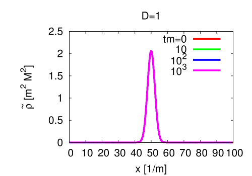
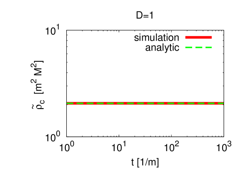
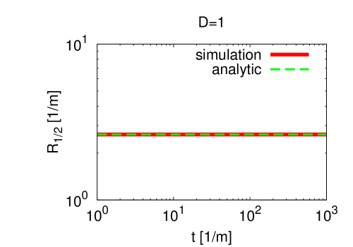
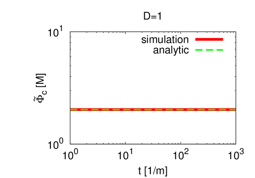
Figure 1: Numerical results of the $I$-ball for $D=1$. We have set $K=10^{-1}$ and $\Phi_{c}=2M$. The top left panel shows snapshots of the spatial distribution of $\tilde{\rho}$ at $t=0,10,10^{2},10^{3}[1/m]$, and all the lines are overlapped, implying that $\tilde{\rho}$ is a constant of motion. The top right, bottom left and bottom right panels show the time evolutions of $\tilde{\rho}_{c}$, $R_{1/2}$ and $\tilde{\Phi}_{c}$ in a very good agreement with the analytic results (59), (60), and (III.1), respectively. The box size is $L=100/m$ and the grid number is $N=2048$.

IV Adiabatic deformation of $I$-balls

In the previous section we have derived the $I$-ball solution so that it minimizes the energy for a given adiabatic charge $I$ in much the same way as $Q$-balls. We have also numerically confirmed that the obtained $I$-ball solution indeed satisfies the equation of motion and the modified energy density remains a constant of motion, which plays a crucial role in the proof of the adiabatic current conservation. In this section, in order to further support the conjecture that the stability (longevity) of the oscillons/$I$-balls is due to the (approximate) conservation of the adiabatic charge, we follow the evolution of the $I$-balls while the coefficient of the logarithmic potential $K$ is varied adiabatically. If the adiabatic invariance indeed guarantees the stability of the $I$-balls, the $I$-ball configuration will be gradually deformed into a Gaussian profile with a different value of $K$, while the adiabatic charge $I$ is conserved.

We introduce the time variation of $K$ as

$$K(t)=\frac{K_{0}}{(1+\alpha mt)},$$ (64)

where $K_{0}$ is the initial value of $K$ at $t=0$, and $\alpha$ is the coefficient of the time variation. For $\alpha\ll 1$, $K$ varies much more slowly than the oscillation period, and therefore, the $I$-ball is expected to evolve into a Gaussian profile with a different value of $K$. Thus, we expect that the $I$-ball radius $R$ and $R_{1/2}$ evolve as

$$R(t)=\sqrt{\frac{2}{K_{0}}}(1+\alpha mt)^{1/2}\frac{1}{m},$$ (65)

$$R_{1/2}=\sqrt{\frac{\ln 2}{K_{0}}}(1+\alpha mt)^{1/2}\frac{1}{m}.$$ (66)

The typical time scale $\Delta t_{R}$ over which the radius $R$ changes significantly is

$$\Delta t_{R}\simeq\left(\frac{\dot{R}}{R}\right)^{-1}=\left(\frac{\alpha m}{2}\frac{1}{1+\alpha mt}\right)^{-1}\simeq\frac{2}{\alpha\,m}.$$ (67)

Therefore we need to follow the evolution of the $I$-balls for a sufficiently long period $(\gg\Delta t_{R})$ in order to see the adiabatic deformation.

How small should $\alpha$ be for the $I$-ball deformation to be adiabatic? To answer this question, let us consider the deformation induced by excitations of the wave packets inside the $I$-ball. The typical time scale for the wave packet to transverse the entire region of the $I$-ball can be estimated as

$$\Delta t_{\delta\phi}\simeq\frac{R}{v_{g}}\simeq\frac{2}{K_{0}\,m},$$ (68)

where $v_{g}$ is the group velocity $v_{g}=\partial\omega/\partial k(k\simeq 1/R)\simeq\sqrt{K_{0}/2}$. For adiabatic deformation of the $I$-ball, this propagation scale $\Delta t_{\delta\phi}$ should be much smaller than $\Delta t_{R}$, i.e., $\Delta t_{\delta\phi}\ll\Delta t_{R}$, which constrains $\alpha$ and $K_{0}$ as

$$\alpha\ll K_{0}.$$ (69)

If this condition (69) is met, the $I$-ball would deform adiabatically.

The adiabatic charge $I$ of the $I$-ball is expected to be conserved during the adiabatic deformation,

$$R_{0}^{D}\Phi_{c,0}^{2}\left(\frac{\overline{\dot{f}^{2}}}{\omega}\right)_{t=0}=R(t)^{D}\Phi_{c}(t)^{2}\left(\frac{\overline{\dot{f}^{2}}}{\omega}\right)_{t=t},$$ (70)

where the subscript $0$ means that the variable is evaluated at $t=0$ (see Eq. (III.1)). As long as $K\ll 1$, the oscillation frequency is given by $m$ up to a correction of order $K$, and so,

$$\left(\frac{\overline{\dot{f}^{2}}}{\omega}\right)_{t=0}=\left(\frac{\overline{\dot{f}^{2}}}{\omega}\right)_{t=t}+{\cal O}(K).$$ (71)

Therefore, the oscillation amplitude at the center, $\Phi_{c}$, should evolve with time as

$$\begin{split}\Phi_{c}(t)&\approx\Phi_{c,0}\left(\frac{R(t)}{R_{0}}\right)^{-D/2}=\Phi_{c,0}(1+\alpha mt)^{-D/4},\end{split}$$ (72)

up to a small correction of order $K$. With this approximation, the effective amplitude $\tilde{\Phi}_{c}$ evolves similarly, $\tilde{\Phi}_{c}(t)\approx\Phi_{c}(t)$ (see Eq. (III.1)).

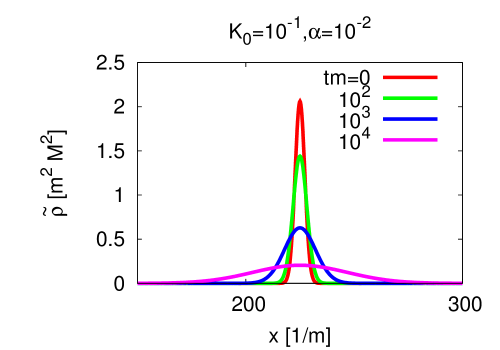
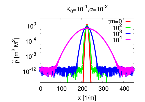
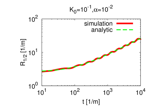
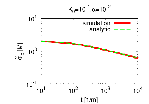
Figure 2: Numerical results for $\alpha=10^{-2}$ and $K_{0}=10^{-1}$ in the case of $D=1$. The top panels show the snapshots of the spatial distribution of $\tilde{\rho}$ at $t=0,10^{2},10^{3},10^{4}[1/m]$ in linear and logarithmic scales. The bottom panels show the evolution of $R_{1/2}$ and $\tilde{\Phi}_{c}$ from $t=10/m$ to $10^{4}[1/m]$. The red (green) line shows the numerical (analytical) result (See Eqs. (66) and (72)).

First let us show the results for the case of $D=1$, where we set the box size $L$ and the number of grid $N$ to

$$L=450/m(t=0),~{}N=2048,~{}\Delta t=10^{-2}\frac{1}{m}.$$ (73)

We have followed the evolution of the $I$-ball from $t=0$ to $t=10^{4}/m$ for $K_{0}=10^{-1}$ and $\alpha=10^{-2}$. As a result the coefficient $K(t)$ evolves from $K_{0}$ to (approximately) $K_{0}/100$, and the $I$-ball radius is expected to become larger by a factor of $10$. In Fig. 2, we show the numerical results. The top two panels show snapshots of the spatial distribution of $\tilde{\rho}$ at $t=0,10^{2},10^{3},10^{4}~{}[1/m]$ with linear and logarithmic scales. One can see that the radius of $I$-ball becomes larger and its amplitude at the center becomes smaller as expected. The two bottom panels show the time evolution of $R_{1/2}$ and $\tilde{\Phi}_{c}$ in a very good agreement with the analytic estimate. This result clearly shows that the adiabatic charge $I$ of the $I$-ball is indeed conserved, and that the $I$-ball configuration follows the analytic solution obtained as the minimal energy state for a given adiabatic charge.

We have similarly studied the deformation of the $I$-balls in the case of $D=2$ and $D=3$ for $K_{0}=10^{-1}$ and $\alpha=10^{-2}$. We set the grid number and the box size as

$$N=256^{2},~{}~{} L=100/m,{\rm~{}~{}for~{}~{}}D=2$$ (74)

$$N=128^{3},~{}~{} L=50/m,{\rm~{}~{}for~{}~{}}D=3$$ (75)

and $\Delta t=10^{-2}/m$ for both cases, and followed the evolution from $t=0$ to $t=10^{3}/m$. The results of the simulations are summarized in Fig. 3. From the top panels, we can see that as the coefficient $K$ becomes smaller, the $I$-ball radius becomes larger. This deformation follows the analytic solutions obtained under the assumption of the adiabatic charge conservation, as can be see from the middle and bottom panels in Fig. 3.

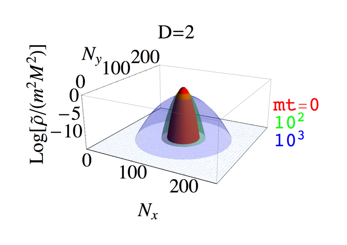
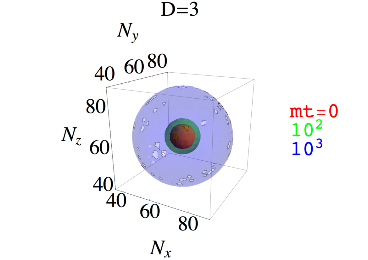
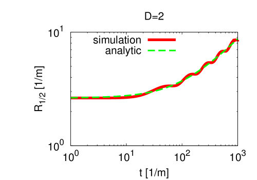
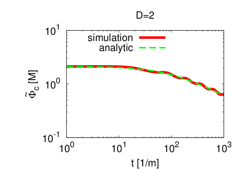
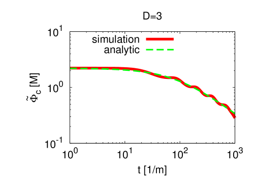
Figure 3: Numerical results for $\alpha=10^{-2}$ and $K_{0}=10^{-1}$ in the cases of $D=2$ and $D=3$. The left (right) panels show the results for $D=2~{}(3)$ case. The top two panels show snapshots of the spatial distribution of $\rho$ at $t=0,10^{2},10^{3}[1/m]$, where $N_{x},N_{y}$ and $N_{z}$ represent the grid point number of the lattice. The middle (bottom) panels show the evolution of $R_{1/2}$ ($\tilde{\Phi}_{c}$) from $t=1/m$ to $10^{3}/m$ in a very good agreement with the analytical ones (66) and (72).

We have confirmed the adiabatic deformation of $I$-balls for $\alpha=10^{-2}$. For a larger $\alpha$, however, the deformation of $I$-ball is no longer adiabatic (see (69)), and it does not follow the analytic profile as the adiabatic charge is not conserved. In Fig. 4, we show the results of the case of $D=1$ with $(K_{0},\alpha)=(10^{-1},10^{-1})$, for which the condition (69) is (marginally) broken. The $I$-ball does not have much time to deform itself in response to the change of $K$. As one can see from Fig. 4, the $I$-ball configuration does not follow the Gaussian profile any more and the evolution of the radius and the amplitude do not match the analytic one.

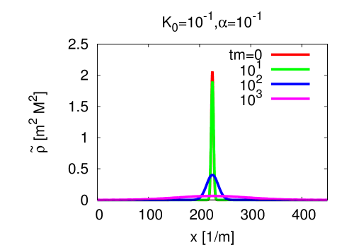
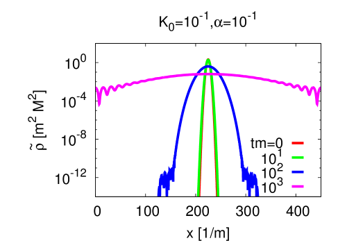
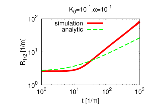
Figure 4: Same as Fig. 2 but for $\alpha=10^{-1}$. The $I$-ball deformation is no longer adiabatic, and it does not follow the analytic one.

V Discussion and conclusions

The longevity of oscillons/$I$-balls was a puzzle, and it was conjectured in Ref. Kasuya:2002zs that it is due to conservation of the adiabatic charge $I$, in much the same way as the $Q$-balls are stable due to conservation of the global U(1) charge $Q$. There, it was numerically confirmed that the $I$-ball field configuration for the LR mass term potential agrees very well with the analytic one derived as the lowest energy state for a given adiabatic charge, giving a strong support for the conjecture.

In this paper we have first proved the adiabatic current conservation for a potential that allows periodic motion with a separable form (11) even in the presence of non-negligible gradient energy. We have found that the modified energy density $\tilde{\rho}$ is a constant of motion, which plays a crucial role in the proof. Then we have determined a possible form of the scalar potential that allows periodic motion to be the LR mass term potential (40). We have derived the $I$-ball solution using the Gaussian ansatz Kasuya:2002zs , under the condition that the adiabatic charge conservation. Finally we have numerically confirmed the evolution and properties of the $I$-balls. In particular, we have followed the adiabatic deformation of the $I$-balls while the coefficient of the logarithmic potential $K$ varies sufficiently slowly with time, and confirmed that the numerical results perfectly agree with the analytic estimates based on the adiabatic charge conservation. We have also checked that, once the adiabatic condition (69) is violated, the $I$-ball starts to spread out and its evolution does not follow the analytic estimate. Thus, our results unambiguously show that the stability (longevity) of the oscillons/$I$-balls is due to the (approximate) conservation of the adiabatic charge.

We have followed the evolution of the $I$-ball starting from the Gaussian solution. As already shown in Ref. Kasuya:2002zs , $I$-balls with the Gaussian profile are formed if one started with the spatial homogeneous initial condition. For $K>0$, there is an instability band, whose growth rate is of order $mK$. Therefore the adiabatic condition is only marginally satisfied. It is of interest to study the adiabatic charge conservation during the $I$-ball formation, and we leave it for future work.

We have focused on the LR mass term potential which enables the periodic motion, making the $I$-ball absolutely stable at the classical level. For the other types of potential dominated by the quadratic potential, the adiabatic charge is approximately conserved. The oscillons/$I$-balls for such potentials are considered to be long-lived due to the approximate conservation of the adiabatic charge. Let us denote the deviation from the LR mass term potential by a small parameter $\epsilon$. The scalar dynamics is no longer given by the separate form (34) because of the deviation. In particular the trajectory over one period is not closed by an amount of $\epsilon$. Noting that the adiabatic invariant in the classical mechanics is a well conserved quantity, and its variation is exponentially suppressed for a small breaking of the adiabaticity Landau , it is plausible that the approximate conservation of the adiabatic charge accounts for the longevity of oscillons observed in various numerical simulations Salmi:2012ta ; Saffin:2006yk ; Graham:2006xs . Intriguingly, it was shown that the oscillons in the small-amplitude regime emit scalar waves in an exponentially suppressed way Fodor:2006zs . The violation of the adiabatic charge may enable us to understand the lifetime of the $I$-ball analytically.

The LR mass term potential (and other types of potentials dominated by the mass term) appears in various cases. For instance, a scalar potential for flat directions in supersymmetric theory is often approximated by such LR mass term potential. The $I$-balls may be formed in the early Universe, and they may play an important cosmological role, especially if they are sufficiently long-lived. In the end of the day the $I$-ball may decay by violation of the adiabatic charge or quantum processes. We leave the cosmological application of the $I$-balls for future work.

References

- (1) I. L. Bogolyubsky and V. G. Makhankov, “On the Pulsed Soliton Lifetime in Two Classical Relativistic Theory Models,” JETP Lett. 24, 12 (1976).
- (2) M. Gleiser, “Pseudostable bubbles,” Phys. Rev. D 49, 2978 (1994) [hep-ph/9308279].
- (3) S. Kasuya, M. Kawasaki and F. Takahashi, “-balls,” Phys. Lett. B 559, 99 (2003) [hep-ph/0209358].
- (4) G. Fodor, P. Forgacs, P. Grandclement and I. Racz, “Oscillons and Quasi-breathers in the phi**4 Klein-Gordon model,” Phys. Rev. D 74, 124003 (2006) [hep-th/0609023].
- (5) E. W. Kolb and I. I. Tkachev, “Nonlinear axion dynamics and formation of cosmological pseudosolitons,” Phys. Rev. D 49, 5040 (1994) [astro-ph/9311037].
- (6) J. McDonald, “Inflaton condensate fragmentation in hybrid inflation models,” Phys. Rev. D 66, 043525 (2002) [hep-ph/0105235].
- (7) M. A. Amin, R. Easther, H. Finkel, R. Flauger and M. P. Hertzberg, “Oscillons After Inflation,” Phys. Rev. Lett. 108, 241302 (2012) [arXiv:1106.3335 [astro-ph.CO]].
- (8) P. Salmi and M. Hindmarsh, Phys. Rev. D 85, 085033 (2012) [arXiv:1201.1934 [hep-th]]; M. Hindmarsh and P. Salmi, Phys. Rev. D 74, 105005 (2006) [hep-th/0606016].
- (9) P. M. Saffin and A. Tranberg, JHEP 0701, 030 (2007) [hep-th/0610191].
- (10) N. Graham and N. Stamatopoulos, Phys. Lett. B 639, 541 (2006) [hep-th/0604134].
- (11) H. Segur and M. D. Kruskal, Phys. Rev. Lett. 58, 747 (1987).
- (12) G. Fodor, P. Forgacs, Z. Horvath and M. Mezei, Phys. Lett. B 674, 319 (2009) [arXiv:0903.0953 [hep-th]]; G. Fodor, P. Forgacs, Z. Horvath and M. Mezei, Phys. Rev. D 79, 065002 (2009) [arXiv:0812.1919 [hep-th]].
- (13) M. Gleiser and D. Sicilia, Phys. Rev. Lett. 101, 011602 (2008) [arXiv:0804.0791 [hep-th]].
- (14) M. P. Hertzberg, Phys. Rev. D 82, 045022 (2010) [arXiv:1003.3459 [hep-th]].
- (15) P. M. Saffin, P. Tognarelli and A. Tranberg, JHEP 1408, 125 (2014) [arXiv:1401.6168 [hep-ph]].
- (16) M. Kawasaki and M. Yamada, JCAP 1402, 001 (2014) [arXiv:1311.0985 [hep-ph]].
- (17) S. R. Coleman, “Q Balls,” Nucl. Phys. B 262, 263 (1985) [Nucl. Phys. B 269, 744 (1986)].
- (18) K. Mukaida and M. Takimoto, JCAP 1408, 051 (2014) [arXiv:1405.3233 [hep-ph]].
- (19) M. Kawasaki, K. Konya and F. Takahashi, Phys. Lett. B 619, 233 (2005) [hep-ph/0504105].
- (20) Y. B. Zeldovich, I. Y. Kobzarev and L. B. Okun, “Cosmological Consequences of the Spontaneous Breakdown of Discrete Symmetry,” Zh. Eksp. Teor. Fiz. 67 (1974) 3 [Sov. Phys. JETP 40 (1974) 1].
- (21) T. W. B. Kibble, “Topology of Cosmic Domains and Strings,” J. Phys. A 9, 1387 (1976).
- (22) L. D. Landau and E. M. Lifshits, Mechanics, 3rd ed. (Butterworth-Hinemann, New York, 1976)/
- (23) Shin’ichiro Tomonaga, “Quantum Mechanics volume 1” (1962), North-Holland publishing company, Amsterdam.