The QBF Gallery: Behind the Scenes

Abstract

Over the last few years, much progress has been made in the theory and practice of solving quantified Boolean formulas (QBF). Novel solvers have been presented that either successfully enhance established techniques or implement novel solving paradigms. Powerful preprocessors have been realized that tune the encoding of a formula to make it easier to solve. Frameworks for certification and solution extraction emerged that allow for a detailed interpretation of a QBF solver’s results, and new types of QBF encodings were presented for various application problems.

To capture these developments the QBF Gallery was established in 2013. The QBF Gallery aims at providing a forum to assess QBF tools and to collect new, expressive benchmarks that allow for documenting the status quo and that indicate promising research directions. These benchmarks became the basis for the experiments conducted in the context of the QBF Gallery 2013 and follow-up evaluations. In this paper, we report on the setup of the QBF Gallery. To this end, we conducted numerous experiments which allowed us not only to assess the quality of the tools, but also the quality of the benchmarks.

1 Introduction

Quantified Boolean formulas (QBF) [10] provide a powerful framework for encoding any application problem located in the complexity class of PSPACE. Many important verification problems like bounded model checking [29] or artificial intelligence tasks like conformance planning [14] can be efficiently encoded as QBF (cf. [3] for a survey). The use of existential and universal quantifiers in QBF potentially allows for encodings which are exponentially more succinct than encodings in propositional logic (SAT). Given the success story of SAT solving [6], much emphasis and efforts have been spent in repeating this success story for QBF, with the aim to avoid the space explosion inherent in SAT encodings. So far, QBF based-technologies have not yet reached the mature state of modern SAT-based technology, but nevertheless continuous progress can be observed.

Recently, several novel approaches emerged ranging from innovative solving techniques to effective preprocessing and new encodings of application problems. A major breakthrough has been achieved by solving the long open problem of calculating certificates for a solver’s result, leading to elegant approaches based on the analysis of resolution proofs [1, 21], to name one example. Such advancements are often distributed over multiple publications and implemented in different tools with evaluations performed within different infrastructures, which makes them hard to compare. Due to this heterogeneity, QBF certainly has some entrance barrier for potential contributors and users. Therefore, we decided to set up the QBF Gallery as annual or biannual event, which is open to all advancements in the field of QBF research.

The first edition of the QBF Gallery was organized in 2013. We invited the QBF research community to contribute ideas on what kind of evaluations would be interesting, given a common infrastructure to perform experiments. The QBF Gallery 2013 [43] was a non-competitive, community-driven event affiliated with the First International Workshop on Quantified Boolean Formulas (QBF 2013). The overall goal was to evaluate the state-of-the-art of QBF-related technologies. This strongly distinguishes the QBF Gallery 2013 event from previous competitions [40, 44], where the main focus was set on the competitive comparison of solvers with the goal to crown winners. In the QBF Gallery 2013, we abstained from this competitive spirit. We were interested in performing comprehensive experiments that allow us to better understand the benefits and drawbacks of different techniques. We did not organize a competition in a traditional sense, so we awarded no prizes. Instead, we collected and analyzed data obtained during numerous experimental runs. The participants were immediately provided with all the results and their feedback was considered for follow-up experiments. Furthermore, in the case of discrepancies in the solving results, we immediately informed the respective participants who could then submit a fix and continue to participate without any consequences. Events like the QBF Gallery are important to give an overview on the state of the art and to provide a common forum for watching the progress in a research community. For potential users, the QBF Gallery should provide an easy entrance into QBF technology by collecting current research results manifesting in tools.

We set up four different showcases for the QBF Gallery 2013. The four showcases are (1) solving, (2) preprocessing, (3) applications, and (4) certification. The solving showcase evaluates and compares different solvers in various scenarios in order to understand the solvers’ suitability for given benchmarks. Naturally, solving also plays an important role in the other showcases. In the preprocessing showcase we were interested in studying the impact of individual and combined preprocessors on the behavior of the solvers. Recently published encodings of application problems, and the ability of the solvers to handle those were studied in the dedicated application showcase. Here, we considered only newly committed benchmarks. Finally, the certification showcase was dedicated to the evaluation of trace producing solvers, and the evaluation of the performance of the certification frameworks. Obviously, the showcases are strongly related and results from one showcase might also be of relevance for the other showcases. However, the different showcases allowed us to focus on different aspects of the solving process.

One piece of feedback we received several times for the organization of the QBF Gallery 2013 was that some important aspect is missing: the competition. Besides the scientific insights, research challenges and documentation of the state of the art, one motivation in participating in a competition is the fun factor and the direct comparison with competitors. Therefore, the participants asked for a competitive setup where prizes are awarded to the best solvers. As a follow-up event of the QBF Gallery 2013, we therefore organized the QBF Gallery 2014 as a traditional solver competition in the context of the FLoC Olympic Games, awarding different medals to the best performing solvers. For the benchmarks, we reused variants of the sets established during the QBF Gallery 2013, which were available to all participants.

In this paper, we take a look behind the scenes of the QBF Gallery 2013 and we report on the experiments which yield the basis for the conducted tool evaluations. To this end, we first summarize the participating systems and the evaluated benchmarks submitted to the QBF Gallery 2013 in Section 2.1. We describe the four different showcases that we considered in our experiments: the solving showcase is presented in Section 3.1, followed by the preprocessing showcase in Section 3.2. In Section 3.3, we report on the application showcase, and finally, in Section 3.4 we give a short summary on the certification showcase. In Section 4, we conclude this paper with a short summary of the QBF Gallery 2014, which was organized as a competition in the context of the FLoC Olympic games. Then we shortly discuss insights gained from the organization of the QBF Gallery and conclude with lessons learned.

2 Setup of the QBF Gallery 2013

In early 2013, we invited the QBF research community to participate in the first edition of the QBF Gallery by contributing ideas, tools, and benchmarks. Overall, 23 contributors from eight countries provided their tools for experiments. The submissions included $15$ solvers for QBFs in conjunctive normal form (CNF), one non-CNF solver, three 2-QBF solvers, four preprocessors, two certification tools, and five new benchmark sets. Besides the newly submitted formulas we additionally considered more than 7,000 formulas provided by the QBFLIB [18], the community portal of QBF researchers. With these artifacts, we performed more than 114,000 runs in over 11,000 CPU hours. Details on the used infrastructure are given with the description of the different experiments. Benchmarks and log files of the runs are available at the website of the QBF Gallery 2013 [43].

At the QBF Gallery event of 2013, we focused on general aspects of tools in the context of QBFs and not only on runtime performance. We set up four showcases where we addressed typical usage scenarios such as solving, preprocessing, novel applications, and strategies/certificates. We tried to identify trends and to gain insights into the performance of the tools. This is very different from previous QBFEVALs, which focused mainly on the competitive aspects in terms of solving performance. On purpose, we decided to use the simplest possible performance metrics like number of solved formulas, average and total runtimes. These simple metrics were sufficient for our goal of understanding how the different systems perform on different benchmark sets. However, in a competitive setting other metrics (cf. for example [45])might have been more adequate.

2.1 Participating Systems and Benchmarks

In this section, we give an overview of the submitted tools and the benchmarks used in the experiments. We provide references to related literature describing the internals of each solvers. The benchmarks are available at the QBF Gallery 2013 website [43].

Tool Name	Submitter(s)	Core Technology
Preprocessors (4)
Hiqqer3e	A. Van Gelder	failed literal detection
Hiqqer3p	A. Van Gelder	univ. expansion, variable elimination
Bloqqer	M. Seidl, A. Biere	univ. expansion, variable elimination
SqueezeBF	M. Narizzano	variable elimination, equivalence rewriting
Solvers (15)
QuBE	M. Narizzano	CDCL
GhostQ	W. Klieber	dual prop.
GhostQ-CEGAR	W. Klieber	dual prop. and CEGAR
bGhostQ-CEGAR	W. Klieber	dual prop., abstraction refinement, Bloqqer
RAReQS	M. Janota	expansion and abstraction refinement (CEGAR)
Hiqqer3	A. Van Gelder	preprocessing and CDCL
Qoq	A. Goultiaeva	CDCL
dual$\_$Ooq	A. Goultiaeva	struct. rec., CDCL, dual prop.
sDual$\_$Ooq	A. Goultiaeva	struct. rec, CDCL, dual prop., preprocessing
Nenofex	F. Lonsing	existential expansion
DepQBF	F. Lonsing	CDCL
DepQBF-lazy-qpup	F. Lonsing	lazy CDCL
free2qbf (2QBF)*	S. Bayless	augmented SAT solver, special decision heuristic
mini2qbf (2QBF)*	S. Bayless	augmented SAT solver
mini2qbf ext. (2QBF)*	S. Bayless	augmented SAT solver, preprocessing
Certification Tools (2)
QBFcert	A. Niemetz,	extraction from resolution proofs
	M. Preiner
ResQu	V. Balabanov,	extraction from resolution proofs
	J.-H. R. Jiang
track skipped

Table 1: Tools and Solvers participating in the QBF Gallery 2013.

2.1.1 Tools

An overview of the submitted tools and contributors is shown in Table 1. The submissions include four preprocessors, 15 solvers as well as two certification tools. Please note that it was allowed to submit up to three different configurations of one tool.

Preprocessors

The goal of preprocessors is to rewrite a formula in prenex conjunctive normal form such that (1) its truth value is not changed and (2) it becomes easier to solve. To this end, preprocessors try to remove irrelevant information and to enhance the formula with additional structure useful for the solving process. Therefore, preprocessing might not only modify and eliminate clauses of a formula, but also add new clauses and even introduce new variables. Four preprocessors were submitted to the QBF Gallery: Bloqqer , Hiqqer3p, Hiqqer3e, and sQueezeBF. They all implement standard optimization techniques like pure and unit literal detection, universal reduction as well as equivalence substitution. Hiqqer3p is a tuned version of Bloqqer [7] that implements variable elimination, universal expansion and blocked clause elimination amongst other techniques. sQueezeBF [17] also uses variable elimination and additionally some special kind of equivalence rewriting that recovers structure lost during the normal form transformation. Hiqqer3e [47] uses an extension of failed literal detection.

Solvers

Table 1 provides an overview of the submitted solvers. The icons shown are later used in the plots to indicate the performance of a solver. Previously, QBF competitions had a CNF track, a non-CNF track as well as a 2-QBF track. We also planned to organize these three different tracks, but due to the lack of submissions in the non-CNF track and the 2-QBF track, we focused on CNF solvers. Solver developers were allowed to submit three variants or configurations of each solver. Four contributors exercised this option, which includes versions of solvers that were enhanced by third-party preprocessors as well. The solver QuBE was the current version of QuBE [16], one of the dominators of the former QBF competitions. The preprocessor sQueezeBF is part of QuBE, where sQueezeBF was also submitted as a standalone tool (see above). The solver QuBE is based on the clause/cube learning (CDCL) variant for QBF. The solver DepQBF [34] also implements clause/cube learning and additionally it considers variable independencies reconstructed from the formula structure to gain more flexibility during the solving process. The variant DepQBF-lazy-qpup [36] uses a different learning approach. The solver Qoq [20] also implements clause and cube learning. Additionally, dual$\_$Ooq implements dual propagation [22] by reconstructing structural information from the CNF. Finally, sDual$\_$Ooq uses the preprocessor sQueezeBF before solving. The solver Hiqqer3 combines the preprocessor Bloqqer with failed literal detection [47]. If the formula is not solved by preprocessing, then an adopted version of the complete solver DepQBF is called. The GhostQ solver [30] aims at overcoming the loss of structural information imposed by the transformation to PCNF by introducing a concept called “ghost variables”. These ghost variables may be considered as a dual variant of the Tseitin variables and provide an efficient mechanism to simulate reasoning on disjunctive normal form. The solver GhostQ-CEGAR [24] extends GhostQ with an additional learning technique based on counterexample-guided abstraction-refinement (CEGAR). The variant bGhostQ-CEGAR calls the preprocessor Bloqqer in certain situations. The solver RAReQS applies CEGAR in an expansion-based approach [24].

Certification Frameworks

QBFcert [39] and ResQu [1] are tool suites to produce Skolem-function models of satisfiable QBFs and Herbrand-function countermodels of unsatisfiable QBFs. To this end, these tools extract a (counter)model from a resolution proof of (un)satisfiability. Since QBFcert and ResQu were the only certification tools submitted, we decided to consider additional publicly available tools and to run additional experiments as presented in Section 3.4.

name	showcase	#	vars∗	clauses∗	alt∗	$\exists^{*}$	$\forall^{*}$
bomb	applications	150	3234	210265	3	3220	14
dungeon	applications	150	36324	264222	3	36318	5
reduction-finding	applications	150	1777	8191	2	1731	44
planning-CTE	applications	150	3239	600112	5	3237	2
qbf-hardness	applications	150	2299	8457	22	2058	100
sauer-reimer	applications	150	13655	40092	3	13407	248
AABBCCDD	preprocessing	234	12060	44516	6	6464	845
AADDBBCC	preprocessing	241	12409	45522	6	6353	816
eval2012r2	solving	345	32924	77709	14	20414	733
eval2012r2 with Bloqqer	solving	276	6834	34938	6	6077	756
eval2010	solving	568	23546	53857	43	18337	223
eval2010 with Bloqqer	solving	420	3532	22578	9	3329	203

Table 2: Formula characteristics of the different benchmark sets: number of formulas (#), average number of variables (vars), average number of clauses (clauses), average number of quantifier alternations (alt), average number of universal/existential variables ($\exists/\forall$).

2.1.2 Benchmarks

In the following, we describe the benchmark sets used in our experiments. New benchmark sets submitted by the participants as well as benchmarks from the public QBFLIB repository were considered. In our experiments, all formulas are in prenex conjunctive normal form (PCNF) with a quantifier prefix having an arbitrary number of quantifier alternations. Details on syntactic formula characteristics are shown in Table 2. For the showcase on applications we selected benchmark sets consisting of 150 formulas each.

• Set eval2010: the complete set of 568 formulas used for QBFEVAL 2010 [40].

• Set eval2012r2: 345 formulas sampled from the collection of formulas available from QBFLIB. This set was also used for the QBF competition QBFEVAL 2012 Second Round, an unofficial repetition of the QBFEVAL 2012 with a new benchmark set.

• Set eval2012r2-inc-preprocessed: Instances from the set eval2012r2 which were obtained by repeated, incremental preprocessing using the four preprocessors that were submitted to the showcase on preprocessing, as described in Section 3.2. We obtained the following two sets:

  • Set AABBCCDD: 234 instances resulting from the set eval2012r2 by incremental preprocessing, where the preprocessors are called in a tool chain in at most six rounds. From the 345 instances, 111 instances were solved during incremental preprocessing. In the tool chain, the formula produced by one preprocessor is forwarded to the next. A wall-clock time limit of 120 seconds was set for each call of a preprocessor. The preprocessors were executed in the ordering AABBCCDD, where “A” is Hiqqer3e, “B” is Bloqqer, “C” is Hiqqer3p, and “D” is SqueezeBF. Fixpoint detection was implemented so that preprocessing stops if the formula is no longer modified by any preprocessor.

  • Set AADDBBCC: 241 instances resulting from the set eval2012r2 by incremental preprocessing. From the 345 instances, 104 instances were solved during preprocessing. This set was generated in similar fashion as the set AABBCCDD except that the execution ordering AADDBBCC was used.

  We selected the execution orderings AABBCCDD and AADDBBCC based on empirical findings we made in the showcase on preprocessing. For example, with ordering AABBCCDD the largest number of instances was solved. Due to the different characteristics of the techniques implemented in Bloqqer (“B”) and SqueezeBF (“D”) we selected AADDBBCC, where SqueezeBF is executed before Bloqqer.

• Set reduction-finding: formulas generated from instances of reduction finding [13, 27, 28], which is the problem to determine whether parametrized quantifier-free reductions exist between various decision problems in NL for one set of fixed parameters. A program to generate this set of benchmarks was also submitted by Charles Jordan and Lukasz Kaiser. The submitted set consists of $4608$ QBF encodings of $2304$ reduction problems, where each problem is encoded as a QBF with prefix $\forall\exists$.

• Set conformant-planning: 1750 instances from a planning domain with uncertainty in the initial state, contributed by Martin Kronegger, Andreas Pfandler, and Reinhard Pichler [31]. The consists of two different kinds of planning problems: dungeon and bomb.

• Set planning-CTE: 150 instances resulting from compact tree encodings (CTE) of planning problems, contributed by Michael Cashmore [12].

• Set sauer-reimer: 924 instances from QBF-based test generation, contributed by Paolo Marin [42].

• Set qbf-hardness: 198 instances from bounded model checking of incomplete designs, contributed by Paolo Marin [38].

• Set samples-eval12r2: ten sets containing 461 formulas each. The formulas in these sets were randomly selected from the instances available in QBFLIB. The random selection process was carried out with respect to families of instances, thus avoiding that instances from large families are overrepresented in the sampled set. In general it can often be observed that solvers perform either very good or very bad on a specific family. Therefore, data accumulated based on benchmark sets which are biased towards particular families is not expressive and may lead to misleading conclusions.

3 Showcases in the QBF Gallery 2013

We invited the participants to suggest the showcases to be considered. At the end, four different showcases were considered: (1) solving, (2) preprocessing, (3) applications, and (4) certification. In the following, we outline the setup of each showcase and summarize the most important results.

3.1 Showcase: Solving

In this showcase, we evaluated the solvers on the benchmark set eval2012r2. We carried out separate runs with and without preprocessing using the preprocessor Bloqqer. All experiments were run on a 64-bit Linux Ubuntu 12.04 system with an Intel Core 2 Quad Q9550@2.83GHz and 8GB of memory. We used a time limit of $900$ seconds and a memory limit of $7$ GB. In the following, we focus on the results obtained for the set eval2012r2. Additional results for the set eval2010, including tables and plots, are reported in B. While some formulas appear in both sets eval2010 and eval2012r2, eval2012r2 contains formulas from more recent benchmark sets.

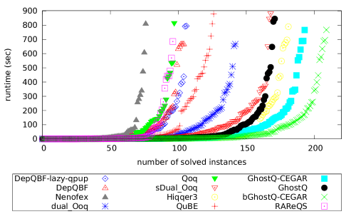
Figure 1: Sorted runtimes of the solvers on the benchmark set eval2012r2 without prior preprocessing using Bloqqer (related to Table 3).

	number of solved formulas				runtime (sec)
solver	solved	sat	unsat	unique	avg	total
bGhostQ-CEGAR	210	111	99	0	50	132K
GhostQ-CEGAR	194	103	91	0	55	146K
Hiqqer3	182	93	89	6	51	156K
GhostQ	172	87	85	2	50	164K
sDual$\_$Ooq	169	80	89	5	63	169K
dual$\_$Ooq	143	66	77	0	58	190K
QuBE	127	60	67	0	93	207K
DepQBF-lazy-qpup	107	43	64	0	63	220K
DepQBF	105	42	63	0	73	223K
Qoq	98	34	64	0	63	228K
RAReQS	97	34	63	5	97	228K
Nenofex	77	34	43	5	53	245K

Table 3: Solving statistics for the set eval2012r2 (345 instances) without prior preprocessing using Bloqqer. Some solvers like dual$\_$Ooq and Hiqqer3, for example, apply built-in preprocessing. The table shows the total number of solved instances (column “solved”), solved satisfiable (column “sat”) and unsatisfiable ones (column “unsat”), uniquely solved instances (column “unique”), and average runtime of solved formulas and total runtime (columns “avg” and “total”) on the whole benchmark set.

Table 3 shows detailed results for the set eval2012r2 without preprocessing. Note that some solvers like dual$\_$Ooq and Hiqqer3, for example, apply built-in preprocessing. Columns “runtime” report the average runtime of solved formulas and the total runtime spent on the entire benchmark set.

This benchmark set is very suitable for search-based solvers such as bGhostQ-CEGAR (and its variants) and Hiqqer3, while the performance of expansion-based solvers like RAReQS and Nenofex is worse. However, both RAReQS and Nenofex solved five unique instances that no other solver could solve. Table 4 presents detailed numbers of solved instances for each benchmark family in the set eval2012r2. Figure 1 shows a cactus plot of the runtimes of the solvers.

We obtain a very different picture of the solver performance when the set eval2012r2 is preprocessed using Bloqqer. In the following experiment, every solver is run on the $276$ instances that were preprocessed but not solved by Bloqqer. Some solvers additionally apply their built-in preprocessors. Table 5 shows the number of successfully solved formulas which, compared to Table 3, gives a very different picture. Notably, RAReQS and DepQBF-lazy-qpup (and its variants) are now more highly ranked than bGhostQ-CEGAR (and its variants). Although Nenofex still solved the smallest number of instances, as in Table 3, it solved eight instances uniquely, which is the largest number of uniquely solved instances among all solvers. Table 6 and Figure 2 show detailed, family-based statistics and runtimes, respectively.

	QuBE	bGhostQ-CEGAR	dual$\_$Ooq	RAReQS	GhostQ-CEGAR	Hiqqer3	GhostQ	DepQBF	Nenofex	sDual$\_$Ooq	Qoq	DepQBF-lazy-qpup
Ansotegui (20)	11	5	6	6	5	10	7	10	0	11	10	10
Ayari (12)	6	5	6	5	0	7	0	0	6	6	4	0
Basler (18)	3	13	1	0	13	6	4	0	0	8	0	0
Biere (16)	5	14	9	1	14	5	14	3	3	6	3	3
gelder (12)	9	12	11	6	12	12	12	11	3	11	10	11
Gent-Rowley (4)	1	1	1	0	1	1	1	1	0	1	1	1
Herbstritt (12)	10	9	10	7	9	9	10	6	1	10	6	6
jiang (12)	2	5	6	1	5	6	5	5	1	6	6	4
Katz (12)	2	0	0	0	0	2	0	0	1	3	0	0
Kontchakov (18)	12	8	16	0	8	18	0	18	0	17	1	18
Lahiri-Seshia (3)	0	2	0	0	2	0	2	0	0	0	0	0
Letombe (6)	6	6	6	6	6	6	6	6	2	6	6	6
Ling (2)	0	2	2	2	2	2	1	2	2	2	2	2
Mangassarian-Veneris (11)	2	4	4	6	4	6	3	5	7	4	4	6
Messinger (6)	0	0	0	0	0	0	0	0	0	0	0	0
Miller-Marin (18)	14	15	12	17	15	17	13	15	12	16	12	16
Mneimneh-Sakallah (38)	15	31	18	0	31	9	31	0	0	16	0	0
Palacios (16)	2	9	5	14	9	5	4	5	9	5	5	4
Pan (48)	10	33	19	6	30	39	30	8	15	22	18	8
Rintanen (12)	2	8	6	10	8	6	8	7	10	5	6	9
sauer$\_$reimer (6)	2	6	2	2	6	4	5	1	0	2	2	1
Scholl-Becker (25)	2	13	3	8	13	3	15	2	4	4	2	2
Wintersteiger (18)	11	9	0	0	1	9	1	0	1	8	0	0
total (345)	127	210	143	97	194	182	172	105	77	169	98	107

Table 4: Numbers of solved instances for each benchmark family in the set eval2012r2 (related to the results reported in Table 3). The number of instances in each family (first column) is shown in parentheses.

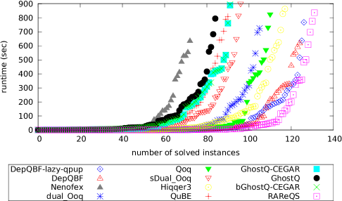
Figure 2: Sorted runtimes of the solvers on the benchmark set eval2012r2 with prior preprocessing using Bloqqer (related to Table 5).

	number of solved formulas				runtime (sec)
solver	solved	sat	unsat	unique	avg	total
RAReQS	132	66	66	7	55	136K
DepQBF-lazy-qpup	127	66	61	0	55	141K
DepQBF	125	66	59	0	55	142K
Hiqqer3	118	59	59	3	82	151K
Qoq	111	58	53	3	58	155K
dual$\_$Ooq	106	57	49	2	58	159K
sDual$\_$Ooq	97	54	43	0	86	169K
GhostQ-CEGAR	92	54	38	0	99	169K
bGhostQ-CEGAR	92	54	38	0	99	174K
QuBE	91	52	39	0	96	175K
GhostQ	85	50	35	0	88	179K
Nenofex	73	39	34	8	77	188K

Table 5: Solving statistics for the set eval2012r2 preprocessed with Bloqqer. After preprocessing, $276$ instances remained unsolved. The ranking of the solvers largely differs from the ranking shown in Table 3 where preprocessing prior to solving was omitted.

	QuBE	bGhostQ-CEGAR	dual$\_$Ooq	RAReQS	GhostQ-CEGAR	Hiqqer3	GhostQ	DepQBF	Nenofex	sDual$\_$Ooq	Qoq	DepQBF-lazy-qpup
Ansotegui (20)	12	9	6	7	9	14	11	12	2	7	13	12
Ayari (6)	0	0	0	0	0	1	0	0	4	0	0	0
Basler (12)	0	0	0	3	0	1	0	0	0	0	5	0
Biere (14)	2	3	3	5	3	3	3	3	3	3	4	4
gelder (6)	6	6	6	6	6	6	6	6	6	6	6	6
Gent-Rowley (4)	1	1	1	0	1	1	1	1	0	1	1	1
Herbstritt (11)	7	0	7	11	0	8	0	9	0	6	8	9
jiang (12)	3	6	6	5	6	6	6	4	2	6	6	6
Katz (12)	1	1	3	0	1	2	2	3	1	3	2	3
Kontchakov (18)	9	2	2	1	2	12	3	18	0	1	1	18
Lahiri-Seshia (3)	0	0	0	0	0	0	0	0	0	0	0	0
Letombe (6)	5	6	6	6	6	6	6	6	1	6	6	6
Ling (2)	2	2	2	2	2	2	2	2	2	2	2	2
Mangassarian-Veneris (10)	3	2	4	5	2	5	3	5	9	4	4	5
Messinger (6)	0	0	0	0	0	0	0	0	0	0	0	0
Miller-Marin (11)	8	11	9	11	11	10	9	9	7	9	9	9
Mneimneh-Sakallah (37)	14	14	30	26	14	9	6	16	3	24	19	15
Palacios (16)	2	5	5	11	5	5	5	5	10	5	5	5
Pan (20)	11	6	6	11	6	12	7	10	7	6	7	9
Rintanen (12)	2	9	4	10	9	8	7	8	10	3	7	9
sauer$\_$reimer (4)	2	3	2	2	3	2	3	2	0	2	2	2
Scholl-Becker (25)	1	6	4	9	6	5	5	6	6	3	4	6
Wintersteiger (9)	0	0	0	1	0	0	0	0	0	0	0	0
total (276)	91	92	106	132	92	118	85	125	73	97	111	127

Table 6: Numbers of solved instances for each benchmark family in the set eval2012r2 preprocessed with Bloqqer (related to the results reported in Table 5). The number of instances in each family (first column) is shown in parentheses.

As illustrated by the different rankings in Tables 3 and 5, the performance of the solvers varies depending on the use of preprocessing. On the original set eval2012r2 solvers with built-in preprocessing outperform solvers that do not have built-in preprocessing, as shown in Table 3. On the preprocessed set eval2012r2, another built-in preprocessing step using Bloqqer might have little effect, cause runtime overhead, and hence harm the performance of a solver. Solvers like dual$\_$Ooq and GhostQ try to reconstruct part of the structure of a CNF formula as a preprocessing step. The purpose of this reconstruction step is to recover the structure that was obscured during the conversion of a non-CNF formula into CNF. Structural information might improve the performance of CNF-based solvers [20, 22]. However, structure reconstruction might be hindered when preprocessing by Bloqqer is applied upfront as in the experiment shown in Table 5. The solver bGhostQ-CEGAR dedicates some of its solving time to run Bloqqer in order to see if Bloqqer is able to solve a formula quickly. If this is not the case, then the original formula is considered for solving and the work spent for the preprocessing was useless.

3.1.1 Preprocessing and Solving: “Best Foot Forward” Analysis

On the one hand, solvers that do not apply built-in preprocessing might perform better on an instance that has been preprocessed using Bloqqer. On the other hand, solvers with built-in preprocessing or structure reconstruction might prefer the original instance.

In order to analyze the performance of the solvers with and without prior preprocessing in more detail, we carried out the following experiments. We ran Bloqqer on all 345 instances in the benchmark set eval2012r2. From all these instances, 276 remained unsolved by Bloqqer. We ran each solver twice: once on the 276 instances after they have been preprocessed by Bloqqer, and once on the respective 276 original instances from the set eval2012r2 without preprocessing. That is, in this experiment we exclude instances from the set eval2012r2 that were solved already by Bloqqer.

We classified the solvers into two categories, depending on the numbers of instances that were solved in these two runs. We classified a solver in the “NO Bloqqer” category if it performs better on the original instances than on the instances that have been preprocessed. If a solver performs better on the preprocessed instances than on the original ones, then we classified it in the “WANT Bloqqer” category.

	Number Solved
Category/	Best	Worst
Solvers	Foot	Foot
NO Bloqqer (solvers perform better without Bloqqer)
bGhostQ-CEGAR	142	93
GhostQ-CEGAR	142	93
GhostQ	122	84
sDual$\_$Ooq	118	99
dual$\_$Ooq	105	89
WANT Bloqqer (solvers perform better with Bloqqer)
RAReQS	132	79
DepQBF-lazy-qpup	128	88
DepQBF	125	86
Hiqqer3	117	113
Qoq	93	65
QuBE	91	90
Nenofex	68	50

Table 7: Classification of solvers into two categories depending on their performance on 276 instances of the set eval2012r2 with (category “WANT Bloqqer”) and without prior preprocessing by Bloqqer (category “NO Bloqqer”). In each of these categories, column “Best Foot” shows the numbers of instances that were solved when choosing to run on preprocessed instances or on original ones, respectively. Column “Worst Foot”, on the contrary, shows the numbers of instances solved when making the opposite choice.

Table 7 shows the final classification of the solvers. In the category “WANT Bloqqer”, the columns “Best Foot” and “Worst Foot” report the numbers of instances that were solved by a solver with and without prior preprocessing by Bloqqer, respectively. In contrast to that, in the category “NO Bloqqer”, these columns report the numbers of instances that were solved by a solver without and with prior preprocessing by Bloqqer, respectively. That is, column “Best Foot” represents the best choice of a solver in terms of solved instances whether to run on the original instances or on the preprocessed ones. Contrary to the best choice, column “Worst Foot” represents the respective worst choice in each category.

It is interesting to note that Hiqqer3 and QuBE do not have much preference whether to run on original instances or on preprocessed ones, because their respective best foot and worst foot statistics differ only by four and one formula(s). Recall that Hiqqer3 includes a modified variant of Bloqqer and that QuBE applies a powerful built-in preprocessor. We obtained different results when considering a different benchmark set (cf. Table 29 in the appendix).

The classification in Table 7 confirms the trend that is indicated by the different rankings of the solvers in Tables 3 and 5. Solvers in the “NO Bloqqer” category like bGhostQ-CEGAR (and its variants) perform better without prior preprocessing and thus are more highly ranked in Table 3 than solvers in the “WANT Bloqqer” category like RAReQS and DepQBF-lazy-qpup. In contrast to that, solvers in the “WANT Bloqqer” category perform better with prior preprocessing and thus dominate the solvers from the “NO Bloqqer” category in the ranking shown in Table 5.

The best-foot-forward analysis presented above revealed that the performance of the solvers might heavily depend on the use of preprocessing when applied before the actual solving. In the related experiments, we preprocessed the instances by a single application of Bloqqer. We could also combine several preprocessing tools like sQueezeBF, for example, with Bloqqer to analyze their combined effects. However, here we decided to focus on Bloqqer since some of the submitted solvers like bGhostQ-CEGAR already apply Bloqqer as a built-in preprocessor. In the showcase on preprocessing to be presented below (Section 3.2), we report on a comprehensive evaluation of several preprocessing tools both independently from solvers and combinations thereof.

Trial 1		Trial 2		Trial 3		Trial 4		Trial 5		Trial 6		Trial 7
BB	312	BB	317	BB	316	BB	315	BB	315	BB	310	BB	319
HH	293	HH	298	HH	300	HH	298	HH	291	HH	290	HH	299
AA	284	AA	285	AA	274	AA	272	AA	279	AA	275	AA	284
CC	274	CC	270	CC	265	CC	270	CC	270	CC	273	CC	274
DD	241	DD	237	DD	236	DD	242	DD	232	DD	241	DD	239
EE	211	EE	211	EE	205	EE	216	EE	208	EE	215	EE	211
GG	204	GG	201	GG	200	GG	202	GG	194	GG	194	GG	207
FF	159	FF	162	FF	161	FF	162	FF	159	FF	156	FF	171

Table 8: Ranking of solvers by numbers of instances solved in seven randomly sampled benchmark sets (trials), each containing 455 instances. Solver names are anonymized using a two-letter code.

Trial 1		Trial 2		Trial 3		Trial 4		Trial 5		Trial 6		Trial 7
BB	637	BB	614	BB	619	BB	625	BB	622	BB	646	BB	605
HH	723	HH	698	HH	693	HH	701	HH	729	HH	734	HH	695
AA	759	AA	753	AA	802	AA	810	AA	781	AA	796	AA	757
CC	798	CC	815	CC	838	CC	816	CC	815	CC	804	CC	799
DD	947	DD	963	DD	969	DD	943	DD	986	DD	947	DD	955
EE	1077	EE	1077	EE	1104	EE	1055	EE	1090	EE	1060	EE	1078
GG	1109	GG	1122	GG	1128	GG	1119	GG	1154	GG	1153	GG	1096
FF	1304	FF	1292	FF	1296	FF	1291	FF	1305	FF	1318	FF	1252

Table 9: Like Table 8, but solvers are ranked according to their penalized average runtime (PAR10).

3.1.2 Stratified Sampling

In addition to the application of preprocessing prior to solving, the actual selection of benchmarks might have an influence on the performance of solvers and hence on the rankings in terms of solved instances. A ranking of solvers obtained by experiments might be skewed if certain families of instances are overrepresented in the benchmark set that underlies the experimental evaluation. In order to analyze the effect of the benchmark selection on the ranking of solvers, we carried out the following sampling experiment.

From all benchmark instances available at QBFLIB, we randomly sampled seven benchmark sets containing 455 instances each in a stratified manner. The stratification consisted of randomly choosing six instances from each benchmark family. Thereby, as noted above, we consider a set of instances a family if this set was classified as such at the time the set was submitted to QBFLIB. The instances in the sampled sets were as contributed by users for use as benchmarks, and we did not apply preprocessing by Bloqqer.

In this experiment, we deliberately do not disclose the actual names of the solvers, but used two-letter names. The intention was to put the focus on the experiment itself (which is the evaluation of the benchmark set) and not on the evaluation of a particular solving technique. Based on the best-foot-forward experiment described above, we selected the eight solvers that solved the largest number of formulas. Our focus was on understanding the effects that different selections of benchmark sets can have on the performance of the solvers. We do not declare a solver as the winner based on any ranking by the numbers of solved instances.

Table 8 shows the rankings of the solvers for each of the seven randomly sampled benchmark sets according to the numbers of solved instances. Rather surprisingly, the rankings are identical for all seven benchmark sets. This also applies to the rankings by the penalized average runtime (PAR10) as shown in Table 9, where runs that timed out after 200 seconds were penalized with $10\cdot 200$ seconds.

Two factors that might have contributed to the rankings in Tables 8 and 9 are the relatively small time out of 200 seconds, and the stratified sampling that makes all the sampled benchmark sets fairly similar to each other. With longer time outs we expect to see more variation. The stratified sampling avoids that instances of certain benchmark families are overrepresented in the final set. Furthermore, solvers that perform particularly well on certain families no longer have an advantage when running on benchmark sets where the selection of instances is biased towards that family. Hence multiple solver runs on benchmark sets that were sampled in a stratified way together with different runtime cutoffs might help to obtain an unbiased ranking of solvers and finally to declare a winner in a competitive setting.

3.2 Showcase: Preprocessing

The purpose of this showcase was to find out how many instances can be solved solely by preprocessing and to analyze the effects of preprocessing on the performance of solvers. The latter is closely related to the showcase on solving (Section 3.1). All experiments in this showcase were run on a 64-bit Linux Ubuntu 12.04 system with four 2.6 GHz 12-core AMD Opteron 6238 CPUs and $512$ GB memory in total. The concrete memory limits varied for the different experiments.

We carried out experiments in two settings: in the first setting, we ran each of the four submitted preprocessors shown in Table 1 individually on a given set of original instances. Then, we compared the sets of instances that were solved by a particular preprocessor. In this experiment, the preprocessors do not interfere with each other, which allows to analyze their individual strengths.

In the second setting, we ran the four preprocessors incrementally in multiple rounds. For example, first preprocessor A is run, and its output, i.e. the preprocessed formula, is forwarded to preprocessor B, the output of B in turn is forwarded to C. Finally D is run on the output of C. Then a new round starts with A,B,C, and D. In this experiment the individual preprocessors influence each other, and hence their combined strengths can be analyzed. Given the number of available preprocessors, there multiple execution sequences like ABCD, ABDC, AABBCCDD, etc. We aimed at a comprehensive evaluation by considering as many execution sequences as possible given the available computational resources. When choosing the execution sequences, we also took the characteristics of the preprocessors into account. For example, it might be beneficial to run Hiqqer3e, which performs unit literal detection, before preprocessors that modify the structure of the formula as structure modifications might be prohibitive for the detection of unit literals.

The time limits used in this showcase were smaller than the ones used in the other showcases. The choice of the time limits for preprocessing was based on the conjecture that if an instance can be solved solely by preprocessing, then it can be solved rather quickly.

3.2.1 Individual Preprocessing

First, we address the question of how many instances can be solved solely by the individual preprocessors. Table 10 shows the results of running the four preprocessors on several benchmark sets described in Section 2.1.2. In these experiments, we used a wall-clock time limit of 300 seconds and a memory limit of $7$ GB.

	Hiqqer3e			Bloqqer			Hiqqer3p			SqueezeBF
	t	s	u	t	s	u	t	s	u	t	s	u
eval2012r2 (345)	19	0	19	69	33	36	77	35	42	11	3	8
qbf-hardness (198)	0	0	0	49	12	37	51	12	39	12	0	12
sauer-reimer (924)	81	0	81	137	24	113	153	29	124	78	9	69
planning-CTE (150)	0	0	0	3	2	1	7	6	1	0	0	0
conf.-planning (1750)	646	0	646	489	11	478	486	12	474	48	0	48
red.-finding (4608)	176	0	176	1496	837	659	1650	924	726	674	326	348

Table 10: Total numbers of instances solved by the four considered preprocessors (columns $t$), and solved satisfiable (columns $s$) and unsatisfiable instances (columns $u$). Each preprocessor was run individually on the benchmark sets. Hence the preprocessors did not influence each other.

Given the statistics in Table 10, the performance of the preprocessors varies with respect to the benchmark set. For example, in the benchmark set conformant-planning, Hiqqer3e solves the largest number of instances whereas Hiqqer3p solves the largest number of instances in the set reduction-finding. Note that by construction Hiqqer3e, unlike the other preprocessors, can only solve unsatisfiable formulas, since it does not apply variable elimination.

Table 11 shows a combination of the statistics from Table 10: an instance is considered to be solved if it was solved by at least one of the four considered preprocessors. Interestingly, the total counts in Table 11 are not always clearly higher than the largest individual count from Table 10. This indicates that there are preprocessors that, regarding their effects, subsume other preprocessors on certain benchmark sets. For example, in the set planning-CTE, all instances that are solved by Bloqqer are also solved by Hiqqer3p.

	$A+B+C+D$
	t	s	u
eval2012r2	87	36	51
qbf-hardness	51	12	39
sauer-reimer	158	29	129
planning-CTE	7	6	1
conf.-planning	757	12	745
red.-finding	1679	940	739

Table 11: Total numbers of instances solved by any individual preprocessor from Table 10 (column $t$), total solved satisfiable (column $s$) and solved unsatisfiable instances (column $u$). In the column header, “A” labels Hiqqer3e, “B” labels Bloqqer, “C” labels Hiqqer3p, and “D” labels SqueezeBF.

Further results including pairwise comparisons of the individual preprocessors can be found at the website of the QBF Gallery 2013.

3.2.2 Incremental Preprocessing

Motivated by the diverse performance of the individual preprocessors illustrated in the previous section, we investigate whether their individual strengths can be combined by incremental preprocessing. To this end, the preprocessors are run in multiple rounds. In our setting, at most six rounds were run for each instance. In each round, the instance preprocessed by one preprocessor is forwarded to another and hence the preprocessors influence each other. If an instance is solved by either preprocessor then the whole run terminates. In the following, “A” labels Hiqqer3e, “B” labels Bloqqer, “C” labels Hiqqer3p, and “D” labels SqueezeBF.

A time limit of 120 seconds was imposed for each individual run of A, B, C, and D. Hence in total, given four preprocessors and six rounds, for each instance we allowed at most 2880 seconds for preprocessing. This time out is much larger than the time out of 900 seconds we chose in the showcases on solving and applications. Our motivation for the showcase on preprocessing was to analyze the power of preprocessing decoupled from solving. Therefore, we decided to allow more time for preprocessing than in a typical setting where a solver is combined with a preprocessor.

If a preprocessor fails to process an instance within the given time limit or if it fails due to any other reason, then its input formula is passed on to the next preprocessor in the execution sequence without any modifications. We considered the benchmark set eval2012r2 and tested all $4!=24$ possible execution sequences of A, B, C, and D.

	eval2012r2
	$t$	$s$	$u$
$(\mathit{ABCD})^{6}$	107	44	63
$(\mathit{ABDC})^{6}$	106	42	64
$(\mathit{ACBD})^{6}$	103	43	60
$(\mathit{ACDB})^{6}$	103	43	60
$(\mathit{ADBC})^{6}$	103	41	62
$(\mathit{ADCB})^{6}$	102	41	61
$(\mathit{BACD})^{6}$	102	41	61
$(\mathit{BADC})^{6}$	102	41	61
$(\mathit{BCAD})^{6}$	101	41	60
$(\mathit{BCDA})^{6}$	103	42	61
$(\mathit{BDAC})^{6}$	101	41	60
$(\mathit{BDCA})^{6}$	99	39	60
$(\mathit{CABD})^{6}$	99	41	58
$(\mathit{CADB})^{6}$	99	40	59
$(\mathit{CBAD})^{6}$	98	40	58
$(\mathit{CBDA})^{6}$	98	40	58
$(\mathit{CDAB})^{6}$	100	41	59
$(\mathit{CDBA})^{6}$	100	40	60
$(\mathit{DABC})^{6}$	102	38	64
$(\mathit{DACB})^{6}$	100	38	62
$(\mathit{DBAC})^{6}$	101	38	63
$(\mathit{DBCA})^{6}$	100	38	62
$(\mathit{DCAB})^{6}$	96	37	59
$(\mathit{DCBA})^{6}$	96	37	59
VBS	119	48	71

Table 12: Numbers of instances solved by one out of 24 possible execution sequences of A, B, C, and D within at most six rounds (column $t$), solved satisfiable (column $s$), and unsatisfiable instances (column $u$), where “A” labels Hiqqer3e, “B” labels Bloqqer, “C” labels Hiqqer3p, and “D” labels SqueezeBF. The results of the virtual best solver (VBS) is shown in the last line.

Table 12 shows the number of instances solved by each execution sequence. Each execution sequence solves more instances than any of the individual preprocessors (Tables 10 and 11). In total, 119 instances where solved by any of the execution sequences, which is 34% of the instances contained in the benchmark set eval2012r2. With individual preprocessing, in total 87 instances (25%) were solved by any of the preprocessors (first line in Table 11). These statistics clearly indicate the benefits of incremental preprocessing in terms of solved instances.

However, the performance of incremental preprocessing is sensitive to the ordering of the preprocessors in an execution sequence. For example, the sequences ABCD and ABDC with the prefix AB solve the largest number of instances (107 and 106, respectively). In contrast to that, the sequences DCAB and DCBA with the prefix DC solve the smallest number of instances (96 each). This difference indicates that the techniques implemented in individual preprocessors might have a negative effect in incremental preprocessing. One preprocessor might destroy the structure of the formula, which in turn might restrict the effects of another preprocessor relying on that structure.

According to the results shown in Table 12, the largest number of instances in the eval2012r2 were solved with the sequence ABCD. Based on this observation, we ran the sequence ABCD on the other benchmark sets for at most six rounds. Table 13 shows the results of these experiments. Except for the set qbf-hardness, incremental preprocessing solves considerably more instances than the individual preprocessors (Table 11). For example, for the sets planning-CTE and conformant-planning, 57% and 23% more instances are solved, respectively.

	$(\mathit{ABCD})^{6}$
	t	s	u
eval2012r2	107	44	63
qbf-hardness	51	12	39
sauer-reimer	180	31	149
planning-CTE	11	8	3
conf.-planning	938	13	925
red.-finding	1855	936	919

Table 13: Incremental preprocessing by running the execution sequence ABCD for at most six rounds. Total numbers of solved instances (columns $t$), solved satisfiable (columns $s$), and unsatisfiable instances (columns $u$), where “A” labels Hiqqer3e, “B” labels Bloqqer, “C” labels Hiqqer3p, and “D” labels SqueezeBF.

In an additional experiment, we tested selected execution sequences from Table 12 on the benchmark set eval2012r2, where each preprocessor is run twice in a row. We selected the sequences to be tested according to the numbers of solved instances shown in Table 12 and the individual characteristics of the preprocessors.

As in the previous experiments, we used a wall-clock time limit of 120 seconds for each individual call of a preprocessor and at most six rounds of incremental preprocessing. The results in Table 14 show a moderate increase in the number of solved instances, except for the sequences $(B^{2}C^{2}D^{2}A^{2})^{6}$ and $(D^{2}A^{2}B^{2}C^{2})^{6}$. These observations indicate that after some time preprocessing reaches a point where little or no progress at all is made. In the following, we analyze situations of this kind.

	eval2012r2
	$t$	$s$	$u$
$(A^{2}B^{2}C^{2}D^{2})^{6}$	111	46	65
$(A^{2}B^{2}D^{2}C^{2})^{6}$	111	45	66
$(A^{2}D^{2}B^{2}C^{2})^{6}$	104	42	62
$(B^{2}C^{2}D^{2}A^{2})^{6}$	103	42	61
$(D^{2}A^{2}B^{2}C^{2})^{6}$	102	38	64
Total	115	48	67

Table 14: Incremental preprocessing with different execution sequences where preprocessors are called twice. For example, the string $(A^{2}B^{2}C^{2}D^{2})^{6}$ indicates the execution sequence AABBCCDD where at most six rounds are run. The table shows the total numbers of solved instances (columns $t$), solved satisfiable (columns $s$), and unsatisfiable instances (columns $u$), where “A” labels Hiqqer3e, “B” labels Bloqqer, “C” labels Hiqqer3p, and “D” labels SqueezeBF.

3.2.3 Detection of Fixpoints

When running incremental preprocessing in multiple rounds, it might happen that an instance is not modified anymore during a round. In this case, a fixpoint has been reached and hence preprocessing can be stopped.

In the experimental evaluation of incremental preprocessing, we implemented the detection of fixpoints as follows. At the beginning of each round, before the first preprocessor in the execution sequence is run, the clause set of the current instance is normalized. Normalization discards tautological clauses and sorts the literals of each clause in the set. Then the set of clauses is sorted using the Linux command line tool sort. An MD5 hash value is computed for this normalized instance using the Linux command line tool openssl. The normalized instance is used only for the computation of the hash value and it is not forwarded to the preprocessors. Hence the detection of fixpoints does not interfere with preprocessing. At the end of the current round, after the last preprocessor in the execution sequence has been run, a hash value is computed for the normalized clause set of the instance produced by the last preprocessor. If the hash values at the beginning and at the end of a round are equal then the clause set was not modified by preprocessing in the current round. Hence a fixpoint has been reached and the run terminates.

Due to normalization as described above, the detection of fixpoints we implemented does not distinguish between instances that differ in terms of the ordering of clauses or the ordering of the literals in the clauses. However, in practice different orderings might have an impact on the performance of the preprocessors as the heuristics internal to a preprocessor might be influenced. In the experimental analysis, we did not analyze the effects of different orderings of clauses or literals.

Table 15 shows statistics on fixpoints and solved instances in each out of six rounds when running the five execution sequences from Table 14 on the set eval2012r2. The vast majority of instances is solved already in the first round. No instances are solved in rounds five and six. The number of fixpoints decreases considerably from round four up to round six. This indicates that it is justified to run a limited number of rounds of incremental preprocessing. For example, in a related experiment (not shown in the tables) where we ran the execution sequence $\mathit{ABCD}$ in at most 12 rounds on the set eval2012r2, no instance was solved in rounds 7–12. Likewise, when increasing the number of rounds to 24, then no instance was solved in rounds 7–24.

	eval2012r2
	Solved Instances							Detected Fixpoints
	1	2	3	4	5	6	$\Sigma$	1	2	3	4	5	6	$\Sigma$
$(A^{2}B^{2}C^{2}D^{2})^{6}$	100	8	2	1	0	0	111	2	52	76	60	14	2	206
$(A^{2}B^{2}D^{2}C^{2})^{6}$	101	7	2	1	0	0	111	1	16	113	58	16	3	207
$(A^{2}D^{2}B^{2}C^{2})^{6}$	96	8	0	0	0	0	104	0	16	137	53	12	0	218
$(B^{2}C^{2}D^{2}A^{2})^{6}$	96	5	1	1	0	0	103	2	46	81	66	14	2	211
$(D^{2}A^{2}B^{2}C^{2})^{6}$	93	8	1	0	0	0	102	2	12	141	49	10	4	218

Table 15: Numbers of instances solved and fixpoints detected in each of six rounds (columns “1,…,6”) and the total number of solved instances and fixpoints (columns ’$\Sigma$’) for the five execution sequences from Table 14.

3.2.4 Solving Performance of Preprocessors

In contrast to the experiments conducted in the case of the best-foot-forward experiments above, in the following we are interested in the effects of applying different combinations of preprocessors in multiple rounds and assess the solving performance of preprocessors. As illustrated by Table 15, the numbers of instances solved by preprocessing using a particular execution sequence is sensitive to the ordering of the preprocessing tools in the sequence. To further analyze this effect, we tested the combination of incremental preprocessing and solving. Thereby, we preprocessed the benchmark set eval2012r2 (345 instances) using the execution sequences $(A^{2}B^{2}C^{2}D^{2})^{6}$ and $(A^{2}D^{2}B^{2}C^{2})^{6}$. This way, we obtained the two new benchmark sets AABBCCDD (234 instances remaining unsolved after preprocessing) and AADDBBCC (241 instances remaining) listed in Section 2.1.2, respectively. We selected the sequence $(A^{2}B^{2}C^{2}D^{2})^{6}$ because it solved the largest number of instances (Table 15) and because $(ABCD)^{6}$ performed best according to Table 12. Since Bloqqer (“B”) and sQueezeBF (“D”) have different characteristics, we additionally selected the sequence $(A^{2}D^{2}B^{2}C^{2})^{6}$ where the ordering of these two preprocessors is swapped and still Bloqqer is executed before Hiqqer3p (“C”). We did not consider the sequence $(A^{2}D^{2}C^{2}B^{2})^{6}$ where only Bloqqer and SqueezeBF are swapped since, according to the results shown in Table 12, the execution ordering $(ADCB)$ solved one instance less than the execution ordering $(ADBC)$ in the sequence $(A^{2}D^{2}B^{2}C^{2})^{6}$ we selected.

Tables 16 and 17 show the performance of solvers on the two benchmark sets. The different rankings of the solvers in the tables indicate that their performance is sensitive to the execution ordering of the preprocessors. Furthermore, the total number of instances solved by preprocessing and by solving is different for the two benchmark sets. For the set AABBCCDD, 111 instances were solved by preprocessing (first line in Table 15) and 92 instances were solved by the best solver (first line in Table 16), giving a total of 203 solved instances. For the set AADDBBCC, 104 instances were solved by preprocessing (third line in Table 15) and 104 by the best solver (first line in Table 17), which gives 208 solved instances in total. That is, although preprocessing alone using the execution sequence $(A^{2}D^{2}B^{2}C^{2})^{6}$ solves fewer instances than when using the sequence $(A^{2}B^{2}C^{2}D^{2})^{6}$, solving performs better on the instances that were preprocessed using the former and results in a higher total number of instances solved by preprocessing and solving.

	number of solved formulas				runtime (sec)
solver	solved	sat	unsat	unique	avg	total
RAReQS	92	57	35	8	35	131K
DepQBF-lazy-qpup	90	52	38	0	87	137K
DepQBF	87	50	37	0	98	140K
Qoq	79	49	30	4	107	145K
Hiqqer3	78	45	33	0	79	147K
dual$\_$Ooq	74	48	26	0	93	147K
bGhostQ-CEGAR	64	46	18	0	127	160K
GhostQ-CEGAR	64	46	18	0	124	149K
GhostQ	57	43	14	0	83	164K
sDual$\_$Ooq	54	37	17	0	103	167K
Nenofex	48	32	16	3	59	170K
QuBE	46	33	13	1	88	173K

Table 16: Related to Figure 3: solver performance on the set AABBCCDD (234 instances)

	number of solved formulas				runtime (sec)
solver	solved	sat	unsat	unique	avg	total
DepQBF-lazy-qpup	104	59	45	0	86	132K
RAReQS	104	59	45	7	54	128K
DepQBF	102	59	43	0	87	134K
Hiqqer3	90	52	38	0	99	144K
Qoq	90	56	34	2	61	141K
dual$\_$Ooq	80	54	26	0	81	151K
sDual$\_$Ooq	64	43	21	0	101	165K
GhostQ	61	43	18	0	92	168K
bGhostQ-CEGAR	59	40	19	0	77	168K
GhostQ-CEGAR	59	40	19	0	78	168K
QuBE	58	37	21	0	56	168K
Nenofex	52	34	18	3	53	172K

Table 17: Related to Figure 3: solver performance on the set AADDBBCC (241 instances)

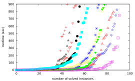
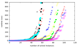
Figure 3: Related to Tables 16 and 17: solver performance on the sets AABBCCDD (left) and AADDBBCC (right). These sets were obtained from the set eval2012r2 by preprocessing using the execution sequences $(A^{2}B^{2}C^{2}D^{2})^{6}$ and $(A^{2}D^{2}B^{2}C^{2})^{6}$, respectively.

3.3 Showcase: Applications

The purpose of the showcase on QBF applications was to evaluate the benchmark families submitted by the participants. The goal was to find out which types of solvers perform well on a specific family, what the reasons are for good or bad performance, and to identify future research directions to improve QBF solvers for benchmark families that arise from practical applications.

From the benchmark sets listed in Section 2.1.2, the following five sets are related to practical applications: reduction-finding, conformant-planning, planning-CTE, sauer-reimer, and qbf-hardness. We split the set conformant-planning into the two subsets conformant-planning-bomb and conformant-planning-dungeon, containing instances with different characteristics. All the formulas considered in this showcase were newly submitted to the QBF Gallery. They have not been used in an evaluation before and are not available from QBFLIB.

From the resulting six sets of application-related benchmarks, we randomly sampled 150 formulas each and tested the submitted solvers on each of these sampled sets. In the following experiments, a time limit of 900 seconds and a memory limit of $7$ GB was used. We did not consider preprocessing in order to evaluate the solvers on the original instances as they were generated by the participants.

Figure 4 shows the run times of the solvers on each set. The plots indicate that the performance of the solvers greatly varies with respect to the benchmark set. Tables 19 to 24 show detailed solving statistics for each of the considered benchmark sets, illustrating the different rankings of the solvers in terms of the numbers of solved formulas. For example, Nenofex clearly outperforms the other solvers on the sets conformant-planning-dungeon and planning-CTE (except RAReQS), but is not competitive on the other sets. This observation is interesting because Nenofex and RAReQS rely on variable expansion. According to the experiments, expansion works particularly well on the considered formulas related to planning problems. On these problems, search-based solvers such as DepQBF, GhostQ-CEGAR, and Hiqqer3, for example, perform considerably worse. However, these solvers perform well on other benchmarks sets like qbf-hardness.

The diverse solver performance on the different application benchmark families as illustrated by Figure 4 motivates exploring potential combinations of the techniques implemented in search-based solvers and expansion-based solvers in future work. The difference in the performance depends on the considered benchmark family. In that respect, the difference is more pronounced in the showcase on applications than in the showcase on solving due to the homogeneity of instances within a particular application benchmark family.

Figure 4: Runtimes of the solvers on six benchmark sets with 150 formulas each related to QBF applications (from top left): conformant-planning-dungeon, conformant-planning-bomb, planning-CTE, sauer-reimer, qbf-hardness, and reduction-finding. In the plots, each color represents a particular solver.

3.4 Showcase: Certificates

The goal of this showcase was to evaluate the current state of the art of the generation of proofs, certificates, and strategies, which has been a long standing problem in QBF research. Proofs, certificates, and strategies allow to verify the result produced by a QBF solver independently from the solving process and provide a deeper insight into the reasons for the (un)satisfiability of a QBF. This insight can be helpful for QBF applications where a mere “SAT/UNSAT” result produced by the solver is insufficient (e.g., QBF-based synthesis [8]).

Given an unsatisfiable QBF $\psi$, a Q-resolution [11] proof of unsatisfiability is a sequence of Q-resolution steps that demonstrates the derivation of the empty clause from $\psi$. If the QBF $\psi$ is satisfiable, then a variant of Q-resolution, called term resolution [19, 32, 49], can be applied to derive the empty cube from $\psi$ by means of a Q-resolution proof of satisfiability. Once a proof $\Pi$ (of unsatisfiability or satisfiability, respectively) has been found for a QBF $\psi$, a strategy [21] or a certificate [1] can be extracted from $\Pi$.

The notion of a strategy is related to the game-oriented view of the semantics of QBF, where the universal and existential player, who assign the universally and existentially quantified variables, try to falsify and satisfy the formula, respectively. Thereby, the two players assign values to the variables in alternating fashion, starting at the left end of the quantifier prefix. The existential (universal) player wins if her selection of values satisfies (falsifies) the formula regardless of the values selected by the other player. A strategy for a satisfiable (unsatisfiable) QBF represents the winning choices of values the existential (universal) player must select depending on the values previously assigned by the universal (existential) player.

A certificate of a satisfiable QBF $\psi$ is a set $F=\{f_{x_{1}}(D_{x_{1}}),\ldots,f_{x_{n}}(D_{x_{n}})\}$ of Skolem functions $f_{x_{i}}(D_{x_{i}})$ for the existential variables $x_{1},\ldots,x_{n}$ of $\psi$. A Skolem function $f_{x_{i}}(D_{x_{i}})$ of an existential variable $x_{i}$ depends on the universal variables $D_{x_{i}}$ that appear to the left of $x_{i}$ in the quantifier prefix of $\psi$. In the process of Skolemization, each occurrence of an existential variable $x_{i}$ in $\psi$ is replaced by its Skolem function $f_{x_{i}}(D_{x_{i}})$. The QBF $\psi^{\prime}$ resulting from Skolemization contains only universal variables and is satisfiable, which can be checked using a propositional satisfiability (SAT) solver by checking whether the negated formula $\neg\psi^{\prime}$ is unsatisfiable. Certificates of unsatisfiable QBFs are defined analogously in terms of Herbrand functions of universal variables. The process of Herbrandization results in an unsatisfiable formula containing only existential variables.

Compared to strategies, which are based on a game-oriented view, certificates in terms of Skolem and Herbrand functions allow for a more explicit, functional representation of values of existential (universal) variables. Apart from that, the concepts of strategies and certificates are similar.

In this showcase, we used the benchmark set eval2012r2 without preprocessing in order to evaluate the generation of proofs and certificates on original instances. Due to the lack of submissions of tools for the generation of strategies, we focused on proofs and certificates. Since only one proof-producing solver (i.e. DepQBF) and only two certificate extraction tools (i.e. ResQu and QBFcert) were officially submitted, we additionally considered further publicly available tools as shown in the lower part of Table 18.

Workflow	Solving+Proof Extr.	Cert. Extr.+Checking
Submitted Tools
DepQBF and QBFcert	91 (34, 57)	67 (20, 47)
DepQBF and ResQu	91 (34, 57)	63 (22, 41)
Additional Tools
sKizzo and ozziKs	88 (36, 52)	35 (35, ​  0)
squolem and qbv	38 (19, 19)	38 (19, 19)
squolem and ResQu	38 (19, 19)	19 (​  0, 19)
QuBE-cert and checker	80 (25, 55)	32 (11, 21)
QuBE-cert and ResQu	80 (25, 55)	52 (17, 35)

Table 18: Experiments with the generation and checking of proofs and certificates using various solvers and tools (first column). After an instances has been solved (second column, numbers of unsatisfiable and satisfiable instances in parentheses), a certificate is extracted and checked (third column, numbers of (un)satisfiable instances where a certificate was successfully extracted and checked). The upper and lower parts of the table, respectively, show the results obtained with officially submitted tools and additional, publicly available tools.

Due to the small number of tools submitted to this showcase, we refrain from ranking the tools according to their performance. Instead, we comment on the results of the experiments shown in Table 18 using various workflows consisting of different solvers and tools for the extraction and checking of certificates.

All experiments were run using a wall-clock time limit of 600 seconds and a memory limit of $3$ GB separately for solving (second column in Table 18) and the checking of proofs and the extraction and checking of the certificates (third column in Table 18).

DepQBF solved and extracted proofs for 91 formulas. For about two thirds of these formulas, the tools QBFcert and ResQu successfully extracted and checked the certificates. These tools implement the same approach to certificate extraction based on Q-resolution proofs [1, 39] and show similar performance. However, the proofs produced by DepQBF had to be converted into a different format supported by ResQu. Both QBFcert and ResQu represent Skolem and Herbrand functions as and-inverter graphs (AIGs). In contrast to QBFcert, the workflow of ResQu includes simplification of AIGs using the tool ABC [9]. We attribute the difference in the number of instances certified by QBFcert and ResQu to the use of ABC. ResQu certified four instances which were not certified by QBFcert, and QBFcert certified eight instances not certified by ResQu.

In the lower part of Table 18, the workflow implemented in QuBE-cert and ResQu is also based on Q-resolution proofs and certificates in terms of Skolem and Herbrand functions and thus is most closely related to DepQBF combined with QBFcert and ResQu. The tool checker does not extract certificates, but only checks the Q-resolution proofs produced by the solver QuBE-cert. The solvers sKizzo and squolem directly extract a certificate out of a given QBF, which is then checked using the tools ozziKs, qbv, or ResQu, respectively. The checker tool ozziKs is designed to check the certificates of satisfiable instances only. Errors were reported on 19 instances solved by squolem when converting the extracted certificates into the input format of ResQu.

For the workflows that involve the extraction of Q-resolution proofs, we observed that not only run time but also memory is critical. For example, when solving an instance, DepQBF writes every Q-resolution step to a trace file stored on the hard disk. This trace file is analyzed by tools like QBFcert and ResQu to extract a certificate. On some instances, the trace file might become very large (up to several gigabytes) as it contains redundant information irrelevant for the proof. The subsequent certificate extraction step might fail due to memory limits. From the 91 instances solved by DepQBF, proofs were extracted from the trace files for 82 instances. The average (median) number of resolution steps in these proofs was 197,472 (2,439), ranging from one to 4,661,201 steps. For the files where the proofs were written to, the average (median) size was 94 MB (1 MB), with a range from 0.003 MB to 1,711 MB.

Our experiments in the showcase on certificates showed that the power of available certification workflows lags behind the power of solvers. That is due to the fact that not every solved instance could be successfully certified within the given time and memory limits. In practice, the size of trace files written by solvers may hinder certification. As a remedy, solvers could maintain resolution proofs directly in memory rather than write trace files to the hard disk. The QRAT proof system [23], for example, may be used to generate proofs in a more compact way than Q-resolution.

4 Conclusions

We presented the experiments we conducted in the context of the QBF Gallery 2013, an event for the evaluation of tools related to QBF solving. In contrast to similar events, the QBF Gallery 2013 was not a competition but it was intended to be a platform for interested researchers to assess the state of the art of QBF technology. In the following, we shortly summarize our findings.

Feedback from the Participants. While all participants agreed that it is important to have a shared forum to be able to compare tools in a uniform setting, it turned out that the involvement of most participants was mainly to provide tools and fixes. There was a moderate discussion ongoing about benchmark selection and related organizational matters. However, the main decisions remained with the organizers. Finally, most participants asked for a competition. The fun factor is a factor that may not be neglected, and especially when prizes are awarded, the motivation is even increased, although the event becomes more of a show than a scientific evaluation.

Benchmark Selection. We performed many experiments to assess the quality of the benchmark sets. We came to the conclusion that the selected sets sufficiently represent the benchmark collection of the QBF research community, which consists of ten thousands of formulas. We received new families of formulas stemming from various kinds of applications. Overall, to compare solvers by their performance it is important that the formulas neither are too easy such that all solvers can solve them nor too hard. We made the benchmarks used available to the community.

Preprocessing and Solving. We used all tools as black boxes as submitted by the authors, i.e., we did not consider other options than the default options of the tools. Overall, we experienced that preprocessing has great impact on the solving performance and that the different preprocessors show diverse performance. Further, it turned out that incremental preprocessing, i.e., multiple applications of a preprocessor until the formula does not change anymore, affects solving performance in a positive way. Further, incremental preprocessing is more powerful than individual preprocessing and the solvers are sensitive to the order in which preprocessors are applied. Although preprocessors usually do not implement complete decision procedures, often they can solve formulas directly. Overall, different solvers perform differently well on different kinds of benchmarks, i.e., the solvers are very sensitive to the structure of the considered problem. This indicates that implementing a hybrid solver based on different solving paradigms might be promising. In the current experiments, we used the preprocessors in the configurations suggested by their authors. However, detailed parameter tuning might further speed up the overall solving process.

We found that on certain novel benchmarks “old” solvers like Nenofex perform very well (cf. [37]). Here a detailed evaluation would be of interest where systems available on the web are collected and run on recently generated encodings. Solvers like Nenofex, Quantor, or sKizzo implement techniques orthogonal to approaches found in currently developed solvers, and explore the search space in a different manner. For combining old and new techniques, hybrid solving or portfolio approaches might be one promising direction of future work (cf. [33, 41]).

4.1 Further Relations to Recent Advances in QBF Proof Complexity

The drastic differences in the performance of solvers on certain benchmark families seem to be related to recent advances in QBF proof complexity. In the QBF Gallery 2013 we did not run experiments to deliberately confirm theoretical results in proof complexity. However, the global picture of our observations to some extent appears to reflect proof theoretical properties of approaches implemented in solvers.

Search-based solvers like QuBE and DepQBF, for example, are based on Q-resolution. Traditional Q-resolution [11] allows to resolve on existential variables and rules out tautological clauses. Long-distance Q-resolution [1, 48] generalizes Q-resolution by permitting the generation of certain tautological resolvents. QU-resolution [46] generalizes Q-resolution by resolving also on universal variables. The proof system LQU$+$resolution [2] combines long-distance Q-resolution and QU-resolution. QU-resolution and long-distance Q-resolution were shown to be stronger than Q-resolution [5, 15, 46]. That is, there are classes of QBFs where any Q-resolution proof is exponentially larger than a proof in QU- or long-distance Q-resolution. Further, LQU$+$resolution was shown to be stronger than QU- and long-distance Q-resolution [2].

From a practical perspective, only Q-resolution and long-distance Q-resolution are applied for QBF solving in a systematic way. Hence the power of stronger proof systems like LQU$+$resolution is still left unused in practice. A variant of DepQBF and the solver Quaffle [48] support long-distance Q-resolution, which however did not participate in the QBF Gallery 2013. QU-resolution [46] is implicitly part of abstraction-based failed-literal detection for QBF [35], as implemented in the preprocessor Hiqqer3e [47]. Hence preprocessing makes QU-resolution available in current solving workflows. This in turn may explain the benefits of preprocessing on solver performance, as QU-resolution is stronger than Q-resolution, which is typically applied in search-based solvers.

Expansion of universal variables is another successful approach to QBF solving, in addition to backtracking search and Q-resolution. A variant of universal expansion was formalized as the proof system $\forall$Exp$+$Res in [25, 26]. Thereby, initially all universal variables are expanded. The resulting propositional formula contains only existential variables and can be solved by Q-resolution. The proof system $\forall$Exp$+$Res was generalized to instantiation of universal variables by truth constants in the proof system IRM-calc [4]. It was shown that IRM-calc polynomially simulates the expansion-based proof system $\forall$Exp$+$Res. That is, for any proof in $\forall$Exp$+$Res there is a proof in IRM-calc that is at most polynomially larger.

It was shown that Q-resolution and $\forall$Exp$+$Res are incomparable with respect to worst-case proof sizes [5, 26]. That is, there are classes of QBFs that have proofs in $\forall$Exp$+$Res of only exponential size but Q-resolution proofs of polynomial size, and vice versa. This theoretical result conforms to our observations made in the experiments conducted in the QBF Gallery 2013. On certain instances, expansion-based solvers clearly outperform search-based solver relying on Q-resolution. For practical QBF solving, it may be worth combining both expansion and Q-resolution in a single solver to benefit from the strengths of both proof systems. So far, the generalized proof systems IRM-calc and LQU$+$resolution [5] have not been implemented in solvers and hence applying them may further improve the state of the art.

4.2 Outlook

Based on the experience gained from the QBF Gallery 2013, one year later, the follow-up event QBF Gallery 2014 was organized in the context of the FLoC Olympic Games. As the 2014 edition of the Gallery was competitive, the organizing team was changed, because here no developer submitting a participating solver should be involved in the organization. Many of the formulas collected for the QBF Gallery 2013 were used in the Gallery $2014$ and from the showcases, three tracks were derived, namely (i) the QBFLIB track, (ii) the Preprocessing track, and (iii) the Application track. Interestingly, all participants who gain benefits from using Bloqqer also submitted their tool with Bloqqer, what is in accordance with the license of version v35. In 2014, no certification track was organized, because although there have been several application papers in 2014 using function extraction facilities for solving their application problems, there are still very few solvers supporting certification.

Acknowledgments

We would like to thank all participants of the QBF Gallery 2013 as well as the participants of the QBF Workshop 2013 for their feedback. Furthermore, we thank the anonymous reviewers for their detailed reports.

Appendix A Tables related to the Showcase on Applications (Section 3.3)

	number of solved formulas				runtime (sec)
solver	solved	sat	unsat	unique	avg	total
RAReQS	102	37	65	5	29	46K
GhostQ-CEGAR	100	50	50	0	31	48K
bGhostQ-CEGAR	100	50	50	0	32	48K
Nenofex	99	56	43	0	21	48K
sDual$\_$Ooq	98	56	42	0	14	48K
Hiqqer3	97	56	41	0	24	50K
GhostQ	92	51	41	0	38	55K
DepQBF	85	43	42	0	51	62K
DepQBF-lazy-qpup	85	43	42	0	41	62K
Qoq	79	37	42	0	14	65K
dual$\_$Ooq	79	37	42	0	14	65K
QuBE	60	24	36	0	66	82K

Table 19: Solving statistics for the set bomb in conformant-planning.

	number of solved formulas				runtime (sec)
solver	solved	sat	unsat	unique	avg	total
Nenofex	149	18	131	36	64	10K
Hiqqer3	107	18	89	0	41	43K
RAReQS	97	18	79	0	26	50K
bGhostQ-CEGAR	92	17	75	0	73	58K
GhostQ-CEGAR	90	17	73	0	157	68K
DepQBF-lazy-qpup	85	18	67	0	15	59K
DepQBF	84	17	67	0	38	62K
GhostQ	84	16	68	0	181	74K
sDual$\_$Ooq	76	9	67	0	288	88K
QuBE	75	6	69	0	143	78K
Qoq	74	8	66	0	356	94K
dual$\_$Ooq	74	8	66	0	356	94K

Table 20: Solving statistics for the set dungeon in conformant-planning.

	number of solved formulas				runtime (sec)
solver	solved	sat	unsat	unique	avg	total
RAReQS	149	40	109	1	30	5K
Nenofex	134	39	95	0	27	18K
DepQBF-lazy-qpup	67	31	36	0	106	81K
Qoq	63	29	34	0	82	83K
DepQBF	60	30	30	0	102	87K
dual$\_$Ooq	59	26	33	0	129	89K
sDual$\_$Ooq	43	27	16	0	134	102K
GhostQ	33	19	14	0	198	111K
Hiqqer3	32	17	15	0	82	108K
bGhostQ-CEGAR	16	9	7	0	339	126K
GhostQ-CEGAR	16	9	7	0	359	126K
QuBE	15	10	5	0	117	123K

Table 21: Solving statistics for the set planning-CTE.

	number of solved formulas				runtime (sec)
solver	solved	sat	unsat	unique	avg	total
DepQBF-lazy-qpup	126	8	118	3	9	22K
DepQBF	125	8	117	2	12	24K
Hiqqer3	123	11	112	2	10	25K
GhostQ	92	10	82	0	24	54K
sDual$\_$Ooq	91	8	83	0	47	57K
GhostQ-CEGAR	87	10	77	0	53	61K
bGhostQ-CEGAR	86	10	76	0	43	61K
QuBE	79	8	71	0	11	64K
dual$\_$Ooq	76	8	68	0	72	72K
RAReQS	49	8	41	0	52	93K
Qoq	40	8	32	0	14	99K
Nenofex	21	8	13	0	18	116K

Table 22: Solving statistics for the set qbf-hardness.

	number of solved formulas				runtime (sec)
solver	solved	sat	unsat	unique	avg	total
RAReQS	121	53	68	10	23	28K
Hiqqer3	100	50	50	0	25	47K
sDual$\_$Ooq	95	44	51	0	30	52K
DepQBF	94	45	49	0	25	52K
DepQBF-lazy-qpup	94	46	48	0	31	53K
Qoq	94	42	52	1	36	53K
dual$\_$Ooq	92	41	51	0	24	54K
bGhostQ-CEGAR	88	35	53	0	37	59K
GhostQ-CEGAR	83	31	52	0	39	63K
QuBE	77	42	35	0	16	67K
GhostQ	67	32	35	0	31	76K
Nenofex	58	29	29	0	6	83K

Table 23: Solving statistics for the set reduction-finding.

	number of solved formulas				runtime (sec)
solver	solved	sat	unsat	unique	avg	total
GhostQ-CEGAR	130	102	28	0	39	23K
bGhostQ-CEGAR	130	102	28	0	40	23K
GhostQ	116	89	27	0	40	35K
Hiqqer3	109	79	30	3	26	39K
sDual$\_$Ooq	77	48	29	0	20	67K
DepQBF	76	51	25	0	24	68K
DepQBF-lazy-qpup	75	51	24	0	19	68K
QuBE	59	33	26	0	38	84K
RAReQS	53	27	26	0	22	88K
Qoq	35	6	29	0	12	103K
dual$\_$Ooq	33	5	28	0	24	106K
Nenofex	18	7	11	0	3	118K

Table 24: Solving statistics for the set sauer-reimer.

Appendix B Tables related to the Showcase on Solving (Section 3.1)

	number of solved formulas				runtime (sec)
solver	solved	sat	unsat	unique	avg	total
Hiqqer3	459	221	238	5	62	126K
sDual$\_$Ooq	417	190	227	0	49	156K
bGhostQ-CEGAR	409	195	214	0	52	164K
dual$\_$Ooq	409	185	224	0	43	161K
GhostQ-CEGAR	400	191	209	0	57	174K
DepQBF-lazy-qpup	395	171	224	0	37	170K
DepQBF	386	167	219	0	31	176K
QuBE	371	161	210	0	68	202K
GhostQ	345	172	173	0	47	217K
Qoq	264	99	165	0	34	282K
RAReQS	258	96	162	3	25	285K
Nenofex	220	106	114	7	25	318K

Table 25: Solving statistics for the set eval2010.

	QuBE	bGhostQ-CEGAR	dual$\_$Ooq	RAReQS	GhostQ-CEGAR	Hiqqer3	GhostQ	DepQBF	Nenofex	sDual$\_$Ooq	Qoq	DepQBF-lazy-qpup
Ansotegui (22)	13	5	7	7	5	13	7	11	0	12	10	12
Ayari (19)	4	5	6	4	1	9	1	2	14	6	3	2
Biere (42)	34	39	23	12	39	22	40	14	8	27	14	14
Castellini (37)	37	37	37	37	37	37	37	37	37	37	37	37
Gent-Rowley (11)	8	8	8	7	8	8	8	8	5	8	8	8
Herbstritt (61)	54	37	45	41	37	45	39	53	11	48	46	54
Katz (3)	3	0	0	0	0	3	0	0	1	3	0	0
Kontchakov (136)	89	75	133	19	75	134	22	136	0	120	13	136
Letombe (52)	50	50	50	50	50	50	51	49	41	51	50	50
Ling (3)	1	3	3	3	3	3	2	3	3	3	3	3
Mangassarian-Veneris (23)	6	14	13	17	13	16	8	12	17	12	13	13
Messinger (3)	1	2	1	2	2	2	1	2	2	1	2	2
Mneimneh-Sakallah (19)	14	18	16	0	18	10	18	0	2	13	0	0
Palacios (15)	3	10	5	14	10	5	4	5	9	5	5	5
Pan (80)	33	74	37	13	71	77	74	27	41	44	36	30
Rintanen (18)	9	16	13	16	15	13	16	16	18	13	13	17
Scholl-Becker (24)	12	16	12	16	16	12	17	11	11	14	11	12
total (568)	371	409	409	258	400	459	345	386	220	417	264	395

Table 26: Detailed solving statistics for the set eval2010.

solver	solved	sat	unsat	unique	avg	total
DepQBF-lazy-qpup	327	164	163	0	49	99K
DepQBF	324	166	158	0	54	104K
Hiqqer3	287	131	156	2	93	146K
RAReQS	250	117	133	12	26	159K
QuBE	227	94	133	1	117	200K
dual$\_$Ooq	201	96	105	0	38	204K
Qoq	196	97	99	0	26	206K
sDual$\_$Ooq	194	97	97	0	73	217K
GhostQ	179	90	89	0	94	233K
GhostQ-CEGAR	179	103	76	0	79	231K
bGhostQ-CEGAR	179	103	76	0	79	231K
Nenofex	123	73	50	7	36	271K

Table 27: Solving statistics for the set eval2010 preprocessed with Bloqqer.

	QuBE	bGhostQ-CEGAR	dual$\_$Ooq	RAReQS	GhostQ-CEGAR	Hiqqer3	GhostQ	DepQBF	Nenofex	sDual$\_$Ooq	Qoq	DepQBF-lazy-qpup
Ansotegui (22)	13	12	7	16	12	14	14	17	3	7	11	17
Ayari (13)	1	1	1	2	1	2	1	1	6	1	1	2
Biere (29)	10	8	8	13	8	13	9	11	5	9	11	12
Castellini (27)	27	27	27	27	27	27	27	27	27	27	27	27
Gent-Rowley (4)	2	1	1	0	1	1	1	1	0	1	1	1
Herbstritt (50)	37	10	38	50	10	39	11	35	1	36	38	37
Katz (3)	3	1	2	1	1	3	2	3	1	2	2	3
Kontchakov (136)	57	23	25	26	23	101	32	136	1	19	14	136
Letombe (29)	27	26	27	28	26	25	27	26	9	27	26	26
Ling (3)	3	3	3	3	3	3	3	3	3	3	3	3
Mangassarian-Veneris (17)	2	9	10	12	9	10	7	10	14	9	10	9
Messinger (3)	1	2	2	3	2	2	1	2	3	2	2	2
Mneimneh-Sakallah (17)	13	11	16	15	11	8	6	12	5	16	14	12
Palacios (14)	2	7	4	11	7	4	5	4	7	4	4	4
Pan (15)	12	9	9	11	9	12	10	11	9	9	9	11
Rintanen (14)	6	13	8	14	13	10	9	11	14	9	10	10
Scholl-Becker (24)	11	16	13	18	16	13	14	14	15	13	13	15
total (420)	227	179	201	250	179	287	179	324	123	194	196	327

Table 28: Detailed solving statistics for the set eval2010 preprocessed with Bloqqer.

	Number Solved
Category/	Best	Worst
Solver	Foot	Foot
NO Bloqqer (solvers perform better without Bloqqer)
Hiqqer3	311	287
dual$\_$Ooq	303	141
sDual$\_$Ooq	302	194
QuBE	268	227
bGhostQ-CEGAR	262	180
GhostQ-CEGAR	262	180
GhostQ	204	179
Qoq	163	142
WANT Bloqqer (solvers perform better with Bloqqer)
DepQBF-lazy-qpup	327	303
DepQBF	323	297
RAReQS	250	184
Nenofex	121	115

Table 29: Classification of solvers into two categories depending on their performance on 568 instances of the set eval2010 with (category “WANT Bloqqer”) and without prior preprocessing by Bloqqer (category “NO Bloqqer”). In each of these categories, column “Best Foot” shows the numbers of instances that were solved when choosing to run on preprocessed instances or on original ones, respectively. Column “Worst Foot”, on the contrary, shows the numbers of instances solved when making the opposite choice.

References

- [1] V. Balabanov and J. R. Jiang. Unified QBF Certification and its Applications. Formal Methods in System Design, 41(1):45–65, 2012.
- [2] V. Balabanov, M. Widl, and J. R. Jiang. QBF Resolution Systems and Their Proof Complexities. In Proc. of the 17th Int. Conference on Theory and Applications of Satisfiability Testing (SAT), 8561 of LNCS, pages 154–169. Springer, 2014.
- [3] M. Benedetti and H. Mangassarian. QBF-Based Formal Verification: Experience and Perspectives. JSAT, 5:133–191, 2008.
- [4] O. Beyersdorff, L. Chew, and M. Janota. On Unification of QBF Resolution-Based Calculi. In Proc. of the 39 Int. Symposium Mathematical Foundations of Computer Science (MFCS), 8635 of LNCS, pages 81–93. Springer, 2014.
- [5] O. Beyersdorff, L. Chew, and M. Janota. Proof Complexity of Resolution-based QBF Calculi. In Proc. of the 32nd Int. Symposium on Theoretical Aspects of Computer Science (STACS), 30 of LIPIcs, pages 76–89. Schloss Dagstuhl - Leibniz-Zentrum fuer Informatik, 2015.
- [6] A. Biere, M. Heule, H. van Maaren, and T. Walsh, editors. Handbook of Satisfiability, 185 of Frontiers in Artificial Intelligence and Applications. IOS Press, 2009.
- [7] A. Biere, F. Lonsing, and M. Seidl. Blocked Clause Elimination for QBF. In Proc. of the 23rd Int. Conference on Automated Deduction (CADE), 6803 of LNCS, pages 101–115. Springer, 2011.
- [8] R. Bloem, R. Könighofer, and M. Seidl. SAT-Based Synthesis Methods for Safety Specs. In Proc. of the 15th Int. Conference on Verification, Model Checking, and Abstract Interpretation (VMCAI), 8318 of LNCS, pages 1–20. Springer, 2014.
- [9] R. K. Brayton and A. Mishchenko. ABC: An Academic Industrial-Strength Verification Tool. In Proc. of the 22nd Int. Conference on Computer Aided Verification (CAV), 6174 of LNCS, pages 24–40. Springer, 2010.
- [10] H. Kleine Büning and U. Bubeck. Theory of Quantified Boolean Formulas. In Handbook of Satisfiability, pages 735–760. IOS Press, 2009.
- [11] H. Kleine Büning, M. Karpinski, and A. Flögel. Resolution for Quantified Boolean Formulas. Inf. Comput., 117(1):12–18, 1995.
- [12] M. Cashmore, M. Fox, and E. Giunchiglia. Planning as Quantified Boolean Formula. In Proc. of the 20th European Conference on Artificial Intelligence (ECAI), 242 of FAIA, pages 217–222. IOS Press, 2012.
- [13] M. Crouch, N. Immerman, and J. Eliot B. Moss. Finding Reductions Automatically. In Fields of Logic and Computation, 6300 of LNCS, pages 181–200. Springer, 2010.
- [14] U. Egly, M. Kronegger, F. Lonsing, and A. Pfandler. Conformant Planning as a Case Study of Incremental QBF Solving. In Proc. of the 12th Int. Conference on Artificial Intelligence and Symbolic Computation (AISC), 8884 of LNCS, pages 120–131. Springer, 2014.
- [15] U. Egly, F. Lonsing, and M. Widl. Long-Distance Resolution: Proof Generation and Strategy Extraction in Search-Based QBF Solving. In Proc. of the 19th Int. Conference on Logic for Programming, Artificial Intelligence, and Reasoning (LPAR), 8312 of LNCS, pages 291–308. Springer, 2013.
- [16] E. Giunchiglia, P. Marin, and M. Narizzano. QuBE7.0. JSAT, 7(2-3):83–88, 2010.
- [17] E. Giunchiglia, P. Marin, and M. Narizzano. sQueezeBF: An Effective Preprocessor for QBFs Based on Equivalence Reasoning. In Proc. of the 13th Int. Conference on Theory and Applications of Satisfiability Testing (SAT), 6175 of LNCS, pages 85–98. Springer, 2010.
- [18] E. Giunchiglia, M. Narizzano, and A. Tacchella. Quantified Boolean Formulas Satisfiability Library (QBFLIB), 2001. http://www.qbflib.org.
- [19] E. Giunchiglia, M. Narizzano, and A. Tacchella. Clause/Term Resolution and Learning in the Evaluation of Quantified Boolean Formulas. J. Artif. Intell. Res. (JAIR), 26:371–416, 2006.
- [20] A. Goultiaeva and F. Bacchus. Recovering and Utilizing Partial Duality in QBF. In Proc. of the 16th Int. Conference on Theory and Applications of Satisfiability Testing (SAT), 7962 of LNCS, pages 83–99. Springer, 2013.
- [21] A. Goultiaeva, A. Van Gelder, and F. Bacchus. A Uniform Approach for Generating Proofs and Strategies for Both True and False QBF Formulas. In Proc. of the 22nd International Joint Conference on Artificial Intelligence (IJCAI). IJCAI/AAAI, 2011.
- [22] A. Goultiaeva, M. Seidl, and A. Biere. Bridging the Gap between Dual Propagation and CNF-based QBF Solving. In Design, Automation and Test in Europe (DATE), pages 811–814. EDA Consortium San Jose / ACM DL, 2013.
- [23] M. Heule, M. Seidl, and A. Biere. A Unified Proof System for QBF Preprocessing. In Proc. of the 7th Int. Joint Conference on Automated Reasoning (IJCAR), 8562 of LNCS, pages 91–106. Springer, 2014.
- [24] M. Janota, W. Klieber, J. Marques-Silva, and E. Clarke. Solving QBF with Counterexample Guided Refinement. In Proc. of the 15th Int. Conference on Theory and Applications of Satisfiability Testing (SAT), 7317 of LNCS, pages 114–128. Springer, 2012.
- [25] M. Janota and J. Marques-Silva. On Propositional QBF Expansions and Q-Resolution. In Proc. of the 16th Int. Conference on Theory and Applications of Satisfiability Testing (SAT), 7962 of LNCS, pages 67–82. Springer, 2013.
- [26] M. Janota and J. Marques-Silva. Expansion-based QBF solving versus Q-resolution. Theor. Comput. Sci., 577:25–42, 2015.
- [27] C. Jordan and L. Kaiser. Benchmarks from Reduction Finding. In QBF Workshop, 2013. http://fmv.jku.at/qbf2013/.
- [28] C. Jordan and L. Kaiser. Experiments with Reduction Finding. In Proc. of the 16th Int. Conference on Theory and Applications of Satisfiability Testing (SAT), 7962 of LNCS, pages 192–207. Springer, 2013.
- [29] T. Jussila and A. Biere. Compressing BMC Encodings with QBF. Electr. Notes Theor. Comput. Sci., 174(3):45–56, 2007.
- [30] W. Klieber, S. Sapra, S. Gao, and E. Clarke. A Non-prenex, Non-clausal QBF Solver with Game-State Learning. In Proc. of the 13th Int. Conference on Theory and Applications of Satisfiability Testing (SAT), 6175 of LNCS, pages 128–142. Springer, 2010.
- [31] M. Kronegger, A. Pfandler, and R. Pichler. Conformant Planning as a Benchmark for QBF-Solvers. In QBF Workshop, 2013. http://fmv.jku.at/qbf2013/.
- [32] R. Letz. Lemma and Model Caching in Decision Procedures for Quantified Boolean Formulas. In Proc. of the Int. Conference on Automated Reasoning with Analytic Tableaux and Related Methods (TABLEAUX), 2381 of LNCS, pages 160–175. Springer, 2002.
- [33] M. T. Lindauer, H. H. Hoos, F. Hutter, and T. Schaub. AutoFolio: An Automatically Configured Algorithm Selector. J. Artif. Intell. Res. (JAIR), 53:745–778, 2015.
- [34] F. Lonsing. Dependency Schemes and Search-Based QBF Solving: Theory and Practice. PhD thesis, Johannes Kepler University, Linz, Austria, 2012.
- [35] F. Lonsing and A. Biere. Failed Literal Detection for QBF. In Proc. of the 14 Int. Conference on Theory and Applications of Satisfiability Testing (SAT), 6695 of LNCS, pages 259–272. Springer, 2011.
- [36] F. Lonsing, U. Egly, and A. Van Gelder. Efficient Clause Learning for Quantified Boolean Formulas via QBF Pseudo Unit Propagation. In Proc. 16th Int. Conference on Theory and Applications of Satisfiability Testing (SAT), 7962 of LNCS, pages 100–115, 2013.
- [37] P. Marin, M. Narizzano, L. Pulina, A. Tacchella, and E. Giunchiglia. An Empirical Perspective on Ten Years of QBF Solving. In Proc. of the 22nd RCRA International Workshop on Experimental Evaluation of Algorithms for Solving Problems with Combinatorial Explosion (RCRA 2015), 1451 of CEUR Workshop Proceedings, pages 62–75. CEUR-WS.org, 2015.
- [38] C. Miller, S. Kupferschmid, M. D. T. Lewis, and B. Becker. Encoding Techniques, Craig Interpolants and Bounded Model Checking for Incomplete Designs. In Proc. of the 13th Int. Conference on Theory and Applications of Satisfiability Testing (SAT), 6175 of LNCS, pages 194–208. Springer, 2010.
- [39] A. Niemetz, M. Preiner, F. Lonsing, M. Seidl, and A. Biere. Resolution-Based Certificate Extraction for QBF - (Tool Presentation). In Proc. of the 15th Int. Conference on Theory and Applications of Satisfiability Testing (SAT), 7317 of LNCS, pages 430–435. Springer, 2012.
- [40] C. Peschiera, L. Pulina, A. Tacchella, U. Bubeck, O. Kullmann, and I. Lynce. The Seventh QBF Solvers Evaluation (QBFEVAL’10). In Proc. of the 13th Int. Conference on Theory and Applications of Satisfiability Testing (SAT), 6175 of LNCS, pages 237–250. Springer, 2010.
- [41] L. Pulina and A. Tacchella. AQME’10. JSAT, 7(2-3):65–70, 2010.
- [42] M. Sauer, S. Reimer, I. Polian, T. Schubert, and B. Becker. Provably Optimal Test Cube Generation using Quantified Boolean Formula Solving. In Proc. of the 18th Asia and South Pacific Design Automation Conference (ASP-DAC), pages 533–539. IEEE, 2013.
- [43] M. Seidl, F. Lonsing, and A. Van Gelder. QBF Gallery 2013 (event website), 2013. http://www.kr.tuwien.ac.at/events/qbfgallery2013/.
- [44] M. Seidl and M. Narizzano. The QBF Evaluation 2012—Round 2, 2013. http://fmv.jku.at/seidl/qbfeval12r2/.
- [45] A. Van Gelder. Careful Ranking of Multiple Solvers with Timeouts and Ties. In Proc. of the 14th Int. Conference on Theory and Applications of Satisfiability Testing (SAT), 6695 of LNCS, pages 317–328. Springer, 2011.
- [46] A. Van Gelder. Contributions to the Theory of Practical Quantified Boolean Formula Solving. In Proc. of the 18th Int. Conference on Principles and Practice of Constraint Programming (CP), 7514 of LNCS, pages 647–663. Springer, 2012.
- [47] A. Van Gelder, S. B. Wood, and F. Lonsing. Extended Failed-Literal Preprocessing for Quantified Boolean Formulas. In Proc. of the 15th Int. Conference on Theory and Applications of Satisfiability Testing (SAT), 7317 of LNCS, pages 86–99. Springer, 2012.
- [48] L. Zhang and S. Malik. Conflict Driven Learning in a Quantified Boolean Satisfiability Solver. In Proc. of the 2002 IEEE/ACM International Conference on Computer-aided Design (ICCAD), pages 442–449. ACM, 2002.
- [49] L. Zhang and S. Malik. Towards a Symmetric Treatment of Satisfaction and Conflicts in Quantified Boolean Formula Evaluation. In Proc. of the 8th Int. Conference on Principles and Practice of Constraint Programming (CP), 2470 of LNCS, pages 200–215. Springer, 2002.