Edge modification criteria for enhancing
the communicability of digraphs

Abstract

We introduce new broadcast and receive communicability indices that can be used as global measures of how effectively information is spread in a directed network. Furthermore, we describe fast and effective criteria for the selection of edges to be added to (or deleted from) a given directed network so as to enhance these network communicability measures. Numerical experiments illustrate the effectiveness of the proposed techniques.

1 Introduction

The concept of network communicability, first introduced by Estrada and Hatano in [9], is being increasingly recognized as an important metric in the structural analysis of networks. The communicability between two nodes $i$ and $j$ is defined as the $(i,j)$th entry in the exponential of the adjacency matrix of the network (or some scaled version of it). This choice can be justified on graph-theoretic grounds based on the concept of walks in a graph, and also from a statistical physics point of view if we regard a network as a system of coupled oscillators and consider the associated thermal Green’s function [10]. To date, there have been a number of applications of communicability to the analysis of real-world complex networks, a few of which are surveyed in [10].

In [3] a new node centrality measure was introduced based on the notion of total communicability, which measures how easily a given node communicates with all the nodes in the network. As pointed out in [3], this centrality measure is closely related to the notion of subgraph centrality [11], while being much easier to compute in the case of large networks. In [3] it was also proposed to use the sum of all the total node communicabilities, possibly normalized by the number of nodes, as a global measure of how effective the network is at propagating information among its nodes. This global index, referred to as total network communicability, was further shown in [1] to provide a good measure of the connectivity and robustness of complex networks, while being much faster to compute than existing metrics (such as the closely related free energy [8] and natural connectivity [26, 27]). Indeed, the cost of estimating the total network communicability using Lanczos-type methods scales linearly in the size of the graph for many types of networks [3].

Given that high communicability is often a highly desirable feature (especially in the case of certain infrastructure, information, and social networks) it is then natural to ask whether it is possible to design networks which are at the same time highly sparse (in the sense of low average degree) and yet have high total communicability. (This problem is analogous to that of constructing good expander graphs, see [20].) In [1] we considered the problem of modifying an existing sparse network so as to cause the total network communicability to change in some desired way. The modification can be the addition of a missing edge, the deletion of an existing edge, or the rewiring of an existing edge. The goal could be to increase the total communicability of the network as much as possible (or nearly so), or to sparsify the network while minimizing the drop in the value of the total communicability, subject to constraints on the number of edge modifications allowed. In [1], several fast and effective heuristics have been developed that achieve the desired goal.

A serious limitation of the notion of total communicability is that it is not well suited to deal with directed networks, and indeed all the above mentioned papers deal exclusively with undirected networks. The main reason is that in a directed graph each node plays two roles, that of broadcaster and that of receiver of information. It is clear that a single index cannot discriminate between these two forms of communication. In this paper, building in part on the ideas in [2], we define two new measures of total network communicability, which quantify how easily information is propagated on a given directed network when the two fundamental modes of communication (broadcasting and receiving) have both to be accounted for. Furthermore, we generalize the edge modification criteria in [1] from the undirected to the directed case, using the newly introduced communicability indices as the objective functions.

Examples of real-world directed networks include various information and citation networks, such as corpora of documents linked to each other by directed edges, for examples hyperlinks between web pages or in-line references between Wikipedia entries. In such networks, one may want to delete edges that contribute little to the overall authoritativeness of the network. In other cases, one may want to add edges from a hub to other nodes so as to increase the overall efficiency of the network in leading to authoritative documents. It is therefore of interest to introduce criteria for edge selection aimed at (approximately) optimizing the global communicability properties of directed networks.

A few other authors have previously considered heuristics for edge manipulation in directed networks. In [28], edge modification criteria are introduced for tuning the synchronizability of a network, a property of interest in many settings. In [13], the authors have considered the potential impact of edge modification on epidemic dynamics on contact networks. It is quite possible that our edge selection criteria may find application in these contexts.

The remainder of the paper is organized as follows. Section 2 contains some background notions about digraphs, the singular value decomposition, and network centrality measures. The new total communicability indices for digraphs are introduced in section 3. The edge updating/downdating problem is described in section 4. In section 5 we introduce the proposed heuristics for edge manipulation, and in section 6 we discuss the result of numerical tests (including timings) using four real-world directed networks. Conclusive remarks are found in section 7.

2 Background

In this section we recall a few definitions and notations associated with graphs. Let $\pazocal{G}=(\pazocal{V},\pazocal{E})$ be a graph with $n=|\pazocal{V}|$ nodes and $m=|\pazocal{E}|$ edges (or links). If for all $i,j\in\pazocal{V}$ such that $(i,j)\in\pazocal{E}$ then also $(j,i)\in\pazocal{E}$, the graph is said to be undirected, as its edges can be traversed without following any prescribed “direction.” On the other hand, if this condition does not hold, namely if there exists $(i,j)\in\pazocal{E}$ such that $(j,i)\not\in\pazocal{E}$, then the network is said to be directed. A directed graph is commonly referred to as a digraph. If $(i,j)\in\pazocal{E}$ in a digraph, we will write $i\rightarrow j$. As for the undirected case, an unweighted digraph can be represented by means of a binary matrix $A\in\mathbb{R}^{n\times n}$ whose entries $(A)_{ij}=a_{ij}$ are nonzero if and only if $(i,j)\in\pazocal{E}$. An ordered pair $(i,j)\not\in\pazocal{E}$ will be called a virtual edge.

Every node $i\in\pazocal{V}$ in a digraph has two types of degree, namely the in-degree and the out-degree; the first, denoted by $d_{in}(i)$, counts the number of edges of the form $*\rightarrow i$, i.e., the number of nodes in $\pazocal G$ from which it is possible to reach $i$ in one step. The out-degree, on the other hand, counts the number of nodes that can be reached from $i$ in one step, i.e., the number of edges of the form $i\rightarrow*$, and is denoted by $d_{out}(i)$. The degrees of a node $i$ can be computed as the $i$th entries of the following two vectors:

$$\left\{\begin{array}[]{l}{\bf d}_{out}=A{\bf 1},\\ {\bf d}_{in}=A^{T}{\bf 1}=({\bf 1}^{T}A)^{T}.\end{array}\right.$$

Here ${\bf 1}$ is the vector of all ones and the superscript “$T$” denotes transposition.

A walk of length $k$ is a sequence of (possibly repeated) nodes $i_{1},i_{2},\ldots,i_{k+1}$ such that $i_{l}\rightarrow i_{l+1}$ for all $l=1,\ldots,k$; a walk is said to be closed if $i_{1}=i_{k+1}$. A path is a walk with no repeated nodes. A digraph is said to be strongly connected if every two nodes in the network are connected through a path of finite length, while it is said to be weakly connected if this property holds when the directionality of the links is disregarded.

Unless otherwise stated, every digraph in this paper is simple, i.e., unweighted, weakly connected, and without self-loops or multi-edges.

Let $A=U\Sigma V^{T}$ be a singular value decomposition (SVD) of the adjacency matrix $A$ [21]. The matrix $\Sigma\in\mathbb{R}^{n\times n}$ is diagonal and its diagonal entries $(\Sigma)_{ii}=\sigma_{i}$ are the singular values of $A$. These elements are non-negative and ordered as

$$\sigma_{1}\geq\sigma_{2}\geq\cdots\geq\sigma_{r}>\sigma_{r+1}=\cdots=\sigma_{n}=0,$$

where $r=\mathop{\operator@font rank}\nolimits(A)$ is the rank of $A$. The matrices $U,V\in\mathbb{R}^{n\times n}$ are orthogonal and $U=[{\bf u}_{1},{\bf u}_{2},\ldots,{\bf u}_{n}]$ contains the left singular vectors of $A$, while $V=[{\bf v}_{1},{\bf v}_{2},\ldots,{\bf v}_{n}]$ contains the right singular vectors. As is well known, $\Sigma$ is uniquely determined by $A$ but $U$ and $V$ are not. Given an SVD of $A$, the corresponding compact singular value decomposition (CSVD) of the matrix $A$ is given by $A=U_{r}\Sigma_{r}V_{r}^{T}$, where $U_{r}=[{\bf u}_{1},{\bf u}_{2},\ldots,{\bf u}_{r}]\in\mathbb{R}^{n\times r}$ and $V_{r}=[{\bf v}_{1},{\bf v}_{2},\ldots,{\bf v}_{r}]\in\mathbb{R}^{n\times r}$ consist of the first $r$ columns of $U$ and $V$, respectively, and $\Sigma_{r}={\rm diag}(\sigma_{1},\sigma_{2},\ldots,\sigma_{r})\in\mathbb{R}^{r\times r}$ corresponds to the leading $r\times r$ diagonal block of $\Sigma$.

2.1 Hubs and authorities

Let us briefly recall here a few definitions concerning the dual role every node plays in a digraph. In [22] Kleinberg stated that in directed networks there exist two types of important nodes: hubs and authorities. In particular, each node can be assigned a hub score and an authority score, which quantify its ability of playing these two roles. Good hubs are those nodes which better broadcast information, while good authorities are those which better receive information. These two types of importance for nodes are strongly related through a recursive definition: the importance of a node as hub is proportional to the importance as authorities of the nodes it points to. Similarly, the importance of a node as authority depends on the importance as hubs of the nodes that point to it. This recursive definition is highlighted in the implementation of the HITS algorithm (see [22]), which makes use of the eigenvectors corresponding to the leading eigenvalue of the symmetric matrices $AA^{T}$ (the hub matrix) and $A^{T}A$ (the authority matrix) to rank the nodes as hubs and authorities, respectively.

Using the SVD or the CSVD of the adjacency matrix, it easily follows that $AA^{T}=U\Sigma^{2}U^{T}=U_{r}\Sigma_{r}^{2}U_{r}^{T}$ and $A^{T}A=V\Sigma^{2}V^{T}=V_{r}\Sigma_{r}^{2}V_{r}^{T}$. Therefore, the vector containing the hub scores is ${\bf u}_{1}$ while the vector containing the authority scores is ${\bf v}_{1}$. By the Perron–Frobenius theorem [21], from the non-negativity and irreducibility of the hub and authority matrices it follows that these principal eigenvectors can be chosen so as to have positive components. Hence, ${\bf u}_{1}>0$ will be called the hub vector and the vector ${\bf v}_{1}>0$ will be called the authority vector.

The powers of the hub and authority matrices are related to the number of particular types of walks in the digraph. Following [2, 6], we define an alternating walk of length $k$ starting with an out-edge as a list of nodes $i_{1},i_{2},\ldots,i_{k+1}$ such that there exists an edge $(i_{l},i_{l+1})$ if $l$ is odd and an edge $(i_{l+1},i_{l})$ if $l$ is even. Hence, an alternating walk starting with an out-edge has the form

$$i_{1}\longrightarrow i_{2}\longleftarrow i_{3}\longrightarrow\ldots.$$

Similarly, an alternating walk of length $k$ starting with an in-edge is a list of nodes $i_{1},i_{2},\ldots,i_{k+1}$ such that

$$i_{1}\longleftarrow i_{2}\longrightarrow i_{3}\longleftarrow\ldots,$$

i.e., such that there exists an edge $(i_{l},i_{l+1})$ if $l$ is even and an edge $(i_{l+1},i_{l})$ otherwise.

It is well known that the entries of powers of the adjacency matrix of a graph can be used to count the number of walks of a certain length in the network. Similarly, it is known (see, e.g., [6]) that $[AA^{T}A\ldots]_{ij}$ (where there are $k$ matrices being multiplied) counts the number of alternating walks of length $k$, starting with an out-edge, from node $i$ to node $j$, whereas $[A^{T}AA^{T}\ldots]_{ij}$ (where there are $k$ matrices being multiplied) counts the number of alternating walks of length $k$, starting with an in-edge, from node $i$ to node $j$. Thus, $[(AA^{T})^{k}]_{ij}$ and $[(A^{T}A)^{k}]_{ij}$ count the number of alternating walks of length $2k$.

In the next section, we will show how to use these quantities to define two global measures of how effectively the nodes in a digraph exchange information.

3 Total network communicabilities for digraphs

In [3] a global measure of how easily information is diffused across an (undirected) network has been defined in terms of the matrix exponential of the adjacency matrix. More in detail, recalling that the entries of the matrix exponential count the total number of walks of any length between two nodes weighting walks of length $k$ by a factor $\frac{1}{k!}$, the total network communicability has been defined as the sum of all the entries of this matrix:

(1) $$TC(A):=\sum_{i=1}^{n}\sum_{j=1}^{n}\left[e^{A}\right]_{ij}={\bf 1}^{T}e^{A}{\bf 1},\quad e^{A}=\sum_{k=0}^{\infty}\frac{1}{k!}A^{k}.$$

This quantity, possibly normalized by $n$, has been empirically shown to provide a good measure of how effectively the information flows along the network and of how well connected an undirected network is (see [1, 3]).

Let now $A$ be the adjacency matrix of a directed graph. In analogy with the undirected case, we can consider the total network communicability (1). In principle, this quantity (possibly normalized by $n$) gives us an idea of how efficient the network is, globally, at diffusing information. However, by following this approach we would be completely disregarding the twofold nature of nodes, which is one of the main features of digraphs.

To better capture the dual behavior of nodes, we introduce two new global indices of communicability defined in terms of functions of the hub and authority matrices.

Definition 1.

Let $A$ be the adjacency matrix of a simple digraph and let $f:{\mathbb{R}}\longrightarrow{\mathbb{R}}$ be a function defined on the spectrum of $AA^{T}$. The total hub $f$-communicability of the digraph is defined as

$$T_{h}C(A,f):={\bf 1}^{T}f(AA^{T}){\bf 1}=\sum_{i=1}^{n}f(\sigma_{i}^{2})({\bf 1}^{T}{\bf u}_{i})^{2}.$$

Similarly, the total authority $f$-communicability of the digraph is defined as

$$T_{a}C(A,f):={\bf 1}^{T}f(A^{T}A){\bf 1}=\sum_{i=1}^{n}f(\sigma_{i}^{2})({\bf 1}^{T}{\bf v}_{i})^{2}.$$

The motivation for using these quadratic forms as total communicability indices is that they exploit the recursive definition that relates hubs and authorities in a directed network. Assume that the function $f$ can be expressed as a power series of the form

(2) $$f(t)=\sum_{k=0}^{\infty}c_{k}t^{k},\quad c_{k}\geq 0\quad\forall k=0,1,\ldots$$

Then, an easy computation shows that the total hub $f$-communicability, can be described in terms of the in-degree vector and of the authority matrix as

$$T_{h}C(A,f)=c_{0}n+c_{1}\|{\bf d}_{in}\|_{2}^{2}+\sum_{k=1}^{\infty}c_{k+1}{\bf d}_{in}^{T}(A^{T}A)^{k}{\bf d}_{in},$$

thus highlighting the fact that the overall ability of nodes to broadcast information depends on their ability of receiving it. Note that due to the nonnegativity assumption on the coefficients in (2), $T_{h}C(A,f)$ is an inherently nonnegative quantity.

Analogous computations carried out on the total authority $f$-communicability show that this index can be completely described in terms of the out-degree vector and of the hub matrix:

$$T_{a}C(A,f)=c_{0}n+c_{1}\|{\bf d}_{out}\|_{2}^{2}+\sum_{k=1}^{\infty}c_{k+1}{\bf d}_{out}^{T}(AA^{T})^{k}{\bf d}_{out},$$

thus showing that the overall ability of nodes to receive information depends on how well they are able to broadcast it. Note that $T_{a}C(A,f)$ is, again, always nonnegative.

Remark 1.

We stress that the total hub and authority $f$-communicabilities are invariant under graph isomorphism. Indeed, let $\pazocal{G}_{1}$ and $\pazocal{G}_{2}$ be two isomorphic graphs with associated adjacency matrices $A_{1}$ and $A_{2}$. Then there exists a permutation matrix $P$ such that $A_{2}=PA_{1}P^{T}$. Therefore,

$$T_{h}C(A_{2},f) ={\bf 1}^{T}f(A_{2}A_{2}^{T}){\bf 1}={\bf 1}^{T}f(PA_{1}P^{T}PA_{1}^{T}P^{T}){\bf 1}$$

$$={\bf 1}^{T}Pf(A_{1}A_{1}^{T})P^{T}{\bf 1}={\bf 1}^{T}f(A_{1}A_{1}^{T}){\bf 1}=T_{h}C(A_{1},f).$$

Similarly,

$$T_{a}C(A_{2},f) ={\bf 1}^{T}f(A_{2}^{T}A_{2}){\bf 1}={\bf 1}^{T}Pf(A_{1}^{T}A_{1})P^{T}{\bf 1}$$

$$={\bf 1}^{T}f(A_{1}^{T}A_{1}){\bf 1}=T_{a}C(A_{1},f).$$

In this paper we will focus on the total hub and authority $f$-communicabilities when the function $f(t)=\cosh(\sqrt{t})$ is used in the definition. The choice of the function $f(t)$ may seem unusual; however, we argue that this choice is the most natural one if one wants to “translate” the idea of total communicability to the case of digraphs. Indeed, in the undirected case the total communicability was defined as the sum of all the entries of the matrix exponential. This index counts all the walks of any length taking place in the network, weighting walks of length $k$ by a factor $\frac{1}{k!}$. In the case of a digraph, we need to count all the alternating walks, again penalizing longer walks. This is accomplished by taking $f(t)=\cosh(\sqrt{t})$; for this choice of $f$ we obtain the total hub communicability as

$$T_{h}C(A) :={\bf 1}^{T}\left(\sum_{k=0}^{\infty}\frac{(AA^{T})^{k}}{(2k)!}\right){\bf 1}={\bf 1}^{T}\left(\sum_{k=0}^{\infty}\frac{(\sqrt{AA^{T}})^{2k}}{(2k)!}\right){\bf 1}$$

$$={\bf 1}^{T}\cosh(\sqrt{AA^{T}}){\bf 1}=T_{h}C(A,\cosh(\sqrt{t})),$$

and, similarly, the total authority communicability as

$$T_{a}C(A) :={\bf 1}^{T}\left(\sum_{k=0}^{\infty}\frac{(A^{T}A)^{k}}{(2k)!}\right){\bf 1}={\bf 1}^{T}\left(\sum_{k=0}^{\infty}\frac{(\sqrt{A^{T}A})^{2k}}{(2k)!}\right){\bf 1}$$

$$={\bf 1}^{T}\cosh(\sqrt{A^{T}A}){\bf 1}=T_{a}C(A,\cosh(\sqrt{t})).$$

A further justification for the choice of the function $f(t)$ comes from considering the following construction (see [2]). Let

(3) $$\mathscr{A}=\left(\begin{array}[]{cc}0&A\\ A^{T}&0\end{array}\right)$$

be the adjacency matrix of the bipartite graph $\mathscr{G}=(\mathscr{V},\mathscr{E})$ obtained from the original digraph represented by $A$. This graph has $2n$ nodes forming the set $\mathscr{V}=\pazocal{V}\cup\pazocal{V}^{\prime}$, where $\pazocal{V}$ is the original set of nodes and $\pazocal{V}^{\prime}=\{1^{\prime}=n+1,2^{\prime}=n+2,\ldots,n^{\prime}=2n\}$ is a set of copies of the nodes in $\pazocal{G}=(\pazocal{V},\pazocal{E})$. The edges between the elements in $\mathscr{V}$ are undirected and $(i,j^{\prime})\in\mathscr{E}$ with $i\in\pazocal{V}$ and $j^{\prime}\in\pazocal{V}^{\prime}$ if and only if $(i,j)\in\pazocal{E}$ in the original digraph.

Note that in the bipartite graph the first $n$ nodes contained in $\pazocal{V}$ can be seen as the original nodes of the digraph when they play their role of broadcasters of information, while the $n$ copies contained in $\pazocal{V}^{\prime}$ represent the original nodes in their role of receivers. It is worth mentioning that the eigenvector of $\mathscr{A}$ corresponding to the leading eigenvalue $\lambda_{1}(\mathscr{A})=\sigma_{1}$ is the vector ${\bf q}_{1}=\left[\begin{array}[]{c}{\bf u}_{1}\\ {\bf v}_{1}\end{array}\right]$. The choice of $f(t)=\cosh(\sqrt{t})$ follows from the next result.

Proposition 2.

[2, Proposition 1] Let $\mathscr{A}$ be as in (3) and let $A=U\Sigma V^{T}$ be an SVD of $A$. Then

(4) $$e^{\mathscr{A}}=\left(\begin{array}[]{cc}\cosh(\sqrt{AA^{T}})&U\sinh(\Sigma)V^{T}\\ V\sinh(\Sigma)U^{T}&\cosh(\sqrt{A^{T}A})\end{array}\right).$$

An important feature of this matrix is that its entries are nonnegative. Thus, these quantities can be used to describe the importance of nodes and how well they communicate when they are acting as broadcasters or receivers of information in the graph [2]. Indeed, the entries of the two diagonal blocks $\cosh(\sqrt{AA^{T}})$ and $\cosh(\sqrt{A^{T}A})$ provide centrality and communicability indices for nodes and pairs of nodes when they are all seen as playing the same role in the network. More in detail, the diagonal entries of the first diagonal block give the centralities for the nodes in the original network when they are seen as broadcasters of information (hubs). Likewise, the diagonal of the second block contains the centralities for the nodes in their role of receivers (authorities). Similarly to the off-diagonal entries of the matrix exponential of an undirected graphs, the off-diagonal entries of these diagonal blocks measure how well two nodes, both acting as broadcasters (resp., receivers), exchange information.

As for the off-diagonal blocks in (4), they contain information concerning how nodes exchange information when one node is playing the role of broadcaster (resp., receiver) and the other is acting as a receiver (resp., broadcaster).

Thus, the total hub communicability and total authority communicability defined as $T_{h}C(A)={\bf 1}^{T}\cosh(\sqrt{AA^{T}}){\bf 1}$ and $T_{a}C(A)={\bf 1}^{T}\cosh(\sqrt{A^{T}A}){\bf 1}$, respectively, account for the overall ability of the network of exchanging information when all its nodes are playing the same role of broadcasters ($T_{h}C(A)$) or receivers ($T_{a}C(A)$).

4 Edge modification strategies

The main goal of this work is to develop heuristics that can be used to add/remove edges from a digraph in order to tune the total hub and/or authority communicability. In particular, we will call update of $(i,j)\not\in\pazocal{E}$ the addition of this virtual edge to the network; we want to perform this operation in such a way that this addition increases as much as possible the quantities of interest. Note that, due to the nonnegativity condition in (2), the addition of an edge can only increase the total communicabilities $T_{h}C(A)$ and $T_{a}C(A)$.

The operation of removing an edge from the network will be referred to as the downdate of an edge. Our aim is to select the edge to be removed in such a way that the target functions $T_{h}C$ and $T_{a}C$ are not penalized too much, i.e., their values do not drop significantly as edges are removed. Both these operations can be described as rank-one modifications of the adjacency matrix $A$ of the digraph $\pazocal G$ or, equivalently, as rank-two modifications of the adjacency matrix $\mathscr{A}$ of the associated bipartite graph $\mathscr{G}$.

We first introduce some edge centrality measures that can be used to rank the (virtual) edges in the digraph; we then use the derived rankings to select which modifications to perform. More in detail, a virtual edge having a large centrality is considered important and thus its addition is expected to highly enhance the total communicabilities. On the other hand, we will remove edges that have a low ranking, since they are not expected to carry a lot of information; thus, their removal is not expected to heavily penalize the hub and authorities communicabilities of the network.

The resulting updating and downdating strategies will be similar in spirit to those adopted in the undirected case [1]. However, as explained in more detail in the next subsection, we cannot simply apply the heuristics in [1] to the bipartite graph $\mathscr{G}$, since doing so could lead to possible loss of structure.

4.1 Bipartite graphs vs. digraphs

In this section we will describe two different ways of tackling the problem of selecting $K$ edge modifications to be performed on the network in order to tune the communicability indices $T_{h}C(A)$ and $T_{a}C(A)$.

First we describe how to rank the edges. A priori, there are two natural approaches. Indeed, given the definitions of communicabilities in terms of the function $f(t)=\cosh(\sqrt{t})$, we can either work on the matrix $\mathscr{A}$ or on the original adjacency matrix $A$. In the first case, we would adapt to the matrix $\mathscr{A}$ the techniques developed for the undirected case which performed best according to the results in [1], taking into account the need to preserve the zero-nonzero block structure of $\mathscr{A}$. The second approach, on the other hand, requires the introduction of new edge centrality measures specially developed for the directed case.

We will show that the new edge centrality measures for digraphs allow us to develop heuristics that perform as well as or better than the techniques for undirected graphs applied to $\mathscr{A}$.

We want to stress here that the set of (virtual) edges among which we select the modifications is the same in both cases, since one wants to preserve the antidiagonal block structure (3) of $\mathscr{A}$. Indeed, if a new edge were to destroy the structure, it could not be “translated” into a new directed edge for the original digraph.

4.2 Edge centralities: undirected case

In the following, we will briefly recall the edge centrality measures introduced in [1] that showed the best performance. These will be used on $\mathscr{A}$ to tackle the updating and downdating problems.

Let $M$ be the adjacency matrix of a simple, undirected graph. We call the edge eigenvector centrality of the (virtual) edge $(i,j)$ the quantity:

$${}^{e}{\pazocal EC}(i,j)=q_{1}(i)q_{1}(j),$$

where $q_{1}(i)$ is the $i$th entry of the Perron vector ${\bf q}_{1}$ of the matrix $M$ (see [21, 5]). We call edge total communicability centrality of $(i,j)$ the quantity:

$${}^{e}{\pazocal TC}(i,j)=(e^{M}{\bf 1})_{i}(e^{M}{\bf 1})_{j}.$$

Let $\lambda_{1}>\lambda_{2}\geq\cdots\geq\lambda_{n}$ denote the eigenvalues of $M$. It has been pointed out that, when the spectral gap $\lambda_{1}-\lambda_{2}$ is large enough, then these two centrality measures provide very similar rankings, especially when the attention is restricted to the top edges; on the other hand, different rankings may be obtained when the gap is small [1, 4].

4.3 Edge centralities: directed case

We now want to define two new edge centrality measures that take into account the directionality of links and that can be computed by directly working on the unsymmetric adjacency matrix $A$.

In [1] it has been pointed out that one of the main factors in the evolution of the total communicability is the dominant eigenvalue $\lambda_{1}$ of the matrix involved in its computation. This is clear since for an undirected graph with adjacency matrix $A$ the total communicability can be expressed as

$$TC(A)=\sum_{i=1}^{n}e^{\lambda_{i}}\alpha_{i}^{2},\quad\alpha_{i}={\bf 1}^{T}{\bf x}_{i},$$

hence the dominant contribution to $TC(A)$ comes from the first term of the sum. Thus, heuristics that increase the spectral radius of $A$ as much as possible will likely be effective also when the goal is to increase the total communicability as much as possible. For example, one of the methods found in [1] to have the best performance relies on the edge eigenvector centrality, which is indeed directly connected to the change that occurs in the magnitude of the leading eigenvalue (see [1] for more details).

Transferring this idea to $T_{h}C(A)$ and $T_{a}C(A)$, it follows that we want to define (if possible) an edge centrality measure that allows us to control the change in the leading singular value of $A$, which corresponds to the square root of the leading eigenvalue of $AA^{T}$ and $A^{T}A$.

Proposition 3.

Let $A$ be the adjacency matrix of a graph. Let ${\bf u}_{1}$ and ${\bf v}_{1}$ be the hub and authority vectors, respectively. Let $\sigma_{1}$ be the leading singular value of $A$. Consider the adjacency matrix of the graph obtained after the addition of the virtual edge $(i,j)$: $\tilde{A}=A+{\bf e}_{i}{\bf e}_{j}^{T}$. Then the leading eigenvalue $\tilde{\sigma}_{1}^{2}$ of the new hub and authority matrices satisfies

(5) $$\tilde{\sigma}_{1}^{2}\geq\sigma_{1}^{2}+2\sigma_{1}u_{1}(i)v_{1}(j)+\max\left\{u_{1}(i)^{2},v_{1}(j)^{2}\right\}.$$

The inequality is strict if $AA^{T}$ is irreducible.

Moreover, let $\widehat{A}=A-{\bf e}_{i}{\bf e}_{j}^{T}$ denote the adjacency matrix obtained after the removal of the existing edge $i\rightarrow j$. Then the leading eigenvalue $\widehat{\sigma}_{1}^{2}$ of the new hub and authority matrices satisfies

(6) $$\sigma_{1}^{2}\geq\widehat{\sigma}_{1}^{2}\geq\sigma_{1}^{2}-2\sigma_{1}u_{1}(i)v_{1}(j)+\max\left\{u_{1}(i)^{2},v_{1}(j)^{2}\right\}.$$

The first inequality is strict if $\widehat{A}\widehat{A}^{T}$ is irreducible.

Proof.

Using the Rayleigh–Ritz Theorem (see, for example, [21]) we get:

$$\tilde{\sigma}_{1}^{2}=\lambda_{1}(\tilde{A}\tilde{A}^{T}) =\max\limits_{\|{\bf z}\|_{2}=1}{\bf z}^{T}\left(\tilde{A}\tilde{A}^{T}\right){\bf z}$$

$$\geq{\bf u}_{1}^{T}\left(\tilde{A}\tilde{A}^{T}\right){\bf u}_{1}$$

$$=\left\|\left(A^{T}+{\bf e}_{j}{\bf e}_{i}^{T}\right){\bf u}_{1}\right\|_{2}^{2}$$

$$=\|\sigma_{1}{\bf v}_{1}+u_{1}(i){\bf e}_{j}\|_{2}^{2}$$

$$=\sigma_{1}^{2}+2\sigma_{1}u_{1}(i)v_{1}(j)+u_{1}(i)^{2}.$$

Similarly, by working on the authority matrix one gets:

$$\tilde{\sigma}_{1}^{2}=\lambda_{1}(\tilde{A}^{T}\tilde{A})\geq{\bf v}_{1}^{T}\left(\tilde{A}^{T}\tilde{A}\right){\bf v}_{1}=\sigma_{1}^{2}+2\sigma_{1}u_{1}(i)v_{1}(j)+v_{1}(j)^{2}.$$

From these inequalities, and from basic facts from Perron–Frobenius theory, the conclusion easily follows. Similar arguments can be used to prove (6).   ∎

Relations (5) and (6) motivate the following definition.

Definition 4.

Let $A$ be the adjacency matrix of a directed graph. Let ${\bf u}_{1}$ and ${\bf v}_{1}$ be its HITS hub and authority vectors, respectively. Then the edge HITS centrality of the existing/virtual edge $(i,j)$ is defined as

$${}^{e}HC(i,j)=u_{1}(i)v_{1}(j).$$

Notice that when $A$ is symmetric this definition reduces to that of edge eigenvector centrality: ${}^{e}EC(i,j)=x_{1}(i)x_{1}(j)$, where ${\bf x}_{1}$ is the eigenvector associated with the leading eigenvalue of $A$.

Remark 2.

Inequalities (5) and (6) and, consequently, definition 4 suggest that there is a “prescribed direction” one has to follow when introducing a new edge centrality measure. Indeed, it is required to use the centrality as broadcaster for the source node $i$ and the centrality as receiver for the target node $j$ when evaluating the importance of the (virtual) edge $i\rightarrow j$. This observation confirms a natural intuition and motivates the usage of this same “orientation” in all our definitions and methods (cf. section 5).

The next edge centrality measure we want to define relies on the use of the total communicability of nodes. Recall that in the case of an undirected network represented by the symmetric adjacency matrix $M$, the total communicability of node $i$ is defined as $(e^{M}{\bf 1})_{i}$. This quantity describes how well node $i$ communicates with the whole network. As discussed in section 3, this centrality measure is well defined for any adjacency matrix, in particular for the adjacency matrices of digraphs, and indeed the row and column sums of $e^{A}$ do provide in some cases meaningful measures of how well nodes broadcast information (row sums of $e^{A}$) and how good they are at receiving information (column sums of $e^{A}$). However, the expressions describing these quantities do not provide information on the alternating walks taking place in the digraph and, thus, miss a crucial feature of communication in real-world directed networks.

For this reason, we introduce here new definitions for the total communicabilities of nodes which can be shown to be directly connected to their twofold nature. In order to do so, we make use of the concept of generalized matrix function first introduced in [18]. Let $A=U_{r}\Sigma_{r}V_{r}^{T}\in{\mathbb{R}}^{n\times n}$ be a matrix of rank $r$, and let $f:{\mathbb{R}}\longrightarrow{\mathbb{R}}$ be a function such that $f(\sigma_{i})$ exists for all $i=1,2,\ldots,r$, so that the matrix function $f(\Sigma_{r})={\rm diag}(f(\sigma_{1}),f(\sigma_{2}),\ldots,f(\sigma_{r}))$ is well defined.

Following [18], we define the generalized matrix function $f^{\diamond}:{\mathbb{R}}^{n\times n}\longrightarrow{\mathbb{R}}^{n\times n}$ as

$$f^{\diamond}(A)=U_{r}f(\Sigma_{r})V_{r}^{T}=\sum_{k=1}^{r}f(\sigma_{k}){\bf u}_{k}{\bf v}_{k}^{T}.$$

It is easy to check that

(7) $$f^{\diamond}(A)=\left(\sum_{k=1}^{r}\frac{f(\sigma_{k})}{\sigma_{k}}{\bf u}_{k}{\bf u}_{k}^{T}\right)A=A\left(\sum_{k=1}^{r}\frac{f(\sigma_{k})}{\sigma_{k}}{\bf v}_{k}{\bf v}_{k}^{T}\right).$$

These equalities show that a generalized matrix function can be expressed in terms of $A$ and either $AA^{T}$ or $A^{T}A$. Therefore, the entries of $f^{\diamond}(A)$ — and hence its row/column sums — can be used as meaningful measures of importance in the directed case, provided that they are all non-negative.

It turns out that, in general, this is not the case for the generalized matrix exponential. Indeed, consider for example the generalized matrix exponential of the adjacency matrix

(8) $$A=\left(\begin{array}[]{cccc}0&0&1&0\\ 1&0&0&1\\ 0&1&0&0\\ 0&1&0&0\end{array}\right)$$

associated with the digraph in Fig. 1. It turns out that its $(3,1)$ and $(4,4)$ entries are negative, and thus these quantities cannot be interpreted as communicability/centrality measures.

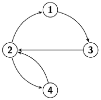
Fig. 1: The digraph associated with adjacency matrix described in (8).

If we instead consider the generalized hyperbolic sine:

$$\sinh^{\diamond}(A)=U_{r}\sinh(\Sigma_{r})V_{r}^{T}=\sum_{k=1}^{r}\sinh(\sigma_{k}){\bf u}_{k}{\bf v}_{k}^{T},$$

we have that this matrix corresponds to the top right block of the matrix $e^{\mathscr{A}}$; indeed, we can rewrite equation (4) as

(9) $$e^{\mathscr{A}}=\left(\begin{array}[]{cc}\cosh(\sqrt{AA^{T}})&\sinh^{\diamond}(A)\\ \sinh^{\diamond}(A)^{T}&\cosh(\sqrt{A^{T}A})\end{array}\right).$$

Hence, the entries of $\sinh^{\diamond}(A)$ are all non-negative, and can be used to quantify how well nodes communicate when they are playing different roles. More precisely, reasoning in terms of alternating walks shows that the $(i,j)$th entry of this matrix describes how well node $i$ exchanges information with node $j$ when the first is playing the role of hub and the latter that of authority. Using this generalized matrix function we can introduce two new centrality measures for nodes in digraphs.

Definition 5.

Let $A=U_{r}\Sigma_{r}V_{r}^{T}$ be the adjacency matrix of a directed network. We call total hub communicability of node $i$ the quantity

(10) $$C_{h}(i)={\bf e}_{i}^{T}\,\sinh^{\diamond}(A)\,{\bf 1}=\sum_{k=1}^{r}\sinh(\sigma_{k})({\bf v}_{k}^{T}{\bf 1})u_{k}(i)$$

and total authority communicability of node $$j$$ the quantity

$$C_{a}(j)={\bf 1}^{T}\,\sinh^{\diamond}(A)\,{\bf e}_{j}=\sum_{k=1}^{r}\sinh(\sigma_{k})({\bf u}_{k}^{T}{\bf 1})v_{k}(j)$$

These quantities correspond to row or column sums of the off-diagonal block of $e^{\mathscr{A}}$; therefore, $C_{h}(i)$ quantifies the ability of node $i$ — playing the role of hub — to communicate with all the nodes in the network, when they are all acting as receivers of information. Similarly, $C_{a}(j)$ accounts for the ability of node $j$ as an authority to receive information from all the nodes in the graph, when they are acting as broadcasters of information. This feature highlights the fact that these definitions are better suited than $e^{A}{\bf 1}$ and $({\bf 1}^{T}e^{A})^{T}$ when it comes to working on digraphs. This result is summarized in the following proposition.

Proposition 6.

Let $A$ be the adjacency matrix of a graph $\pazocal{G}=(\pazocal{V},\pazocal{E})$. The total hub communicability of node $i\in\pazocal{V}$ can be written as

(11a) $$C_{h}(i)=\sum_{k=1}^{r}\frac{\sinh(\sigma_{k})}{\sigma_{k}}{\bf e}_{i}^{T}({\bf u}_{k}{\bf u}_{k}^{T}){\bf d}_{out}=\sum_{k=1}^{r}\frac{\sinh(\sigma_{k})}{\sigma_{k}}({\bf v}_{k}^{T}{\bf 1})\sum_{\begin{subarray}{c}\ell\in\pazocal{V}\\ i\rightarrow\ell\end{subarray}}v_{k}(\ell).$$

Similarly, the total authority communicability of node $$j\in\pazocal{V}$$ can be expressed as

(11b) $$C_{a}(j)=\sum_{k=1}^{r}\frac{\sinh(\sigma_{k})}{\sigma_{k}}{\bf d}_{in}^{T}({\bf v}_{k}{\bf v}_{k}^{T}){\bf e}_{j}=\sum_{k=1}^{r}\frac{\sinh(\sigma_{k})}{\sigma_{k}}({\bf 1}^{T}{\bf u}_{k})\sum_{\begin{subarray}{c}\ell\in\pazocal{V}\\ \ell\rightarrow j\end{subarray}}u_{k}(\ell).$$

Proof.

Using the first equality in (7) one gets that:

$$C_{h}(i) ={\bf e}_{i}^{T}\left(\sum_{k=1}^{r}\frac{\sinh(\sigma_{k})}{\sigma_{k}}{\bf u}_{k}{\bf u}_{k}^{T}\right)A{\bf 1}=\sum_{k=1}^{r}\frac{\sinh(\sigma_{k})}{\sigma_{k}}{\bf e}_{i}^{T}\left({\bf u}_{k}{\bf u}_{k}^{T}\right){\bf d}_{out},$$

which proves the first equality of (11a). To prove the second, we apply the second equality in (7):

$$C_{h}(i) =({\bf e}_{i}^{T}A)\left(\sum_{k=1}^{r}\frac{\sinh(\sigma_{k})}{\sigma_{k}}{\bf v}_{k}{\bf v}_{k}^{T}\right){\bf 1}=\sum_{k=1}^{r}\frac{\sinh(\sigma_{k})}{\sigma_{k}}({\bf v}_{k}^{T}{\bf 1})A_{i,:}{\bf v}_{k},$$

where $A_{i,:}$ is the $i$th row of the adjacency matrix $A$. The conclusion then follows from the fact that $A_{i,:}{\bf v}_{k}=\sum_{i\rightarrow\ell}v_{k}(\ell)$. The proof of (11b) goes along the same lines and is thus omitted.  ∎

Before proceeding with the introduction of the associated edge centrality measure, we want to show with a small example that these measures of hub and authority centrality are indeed informative. Consider as an example the graph in Fig. 1. It is intuitive that node $2$ should be given the highest score both as hub and as authority by any reasonable centrality measure. Consequently, the authority scores for nodes $1$ and $4$ should be the same and higher than that of node $3$ because these nodes are directly pointed to from node $2$, which is the best hub in the graph. For a similar reason, nodes $3$ and $4$ should be ranked higher than node $1$ when considering a hub score, since they directly point to node $2$, which is the most important authority.

Table 1: Centrality measures for the nodes in the graph represented in Fig. 1 and described by the adjacency matrix (8).

NODE	$d_{out}(i)$	$d_{in}(i)$	$u_{1}(i)^{2}$	$v_{1}(i)^{2}$	$C_{h}(i)$	$C_{a}(i)$
1	1	1	.0000	.3333	1.1752	1.3683
2	2	2	.5000	.3333	2.7366	2.7366
3	1	1	.2500	.0000	1.3683	1.1752
4	1	1	.2500	.3333	1.3683	1.3683

Table 1 contains the centrality scores for the four nodes when the in/out-degree, HITS centrality, and the total hub/authority communicability are considered. Clearly, the in/out-degrees of the nodes do not capture the picture we just described since they cannot discriminate between nodes 1, 3, and 4. This happens because the degree centralities take into account only local information about how nodes propagate information in the network.

Concerning HITS, the rankings given by the hub scores conform to our expectations, but those given by the authority scores do not, since they are unable to identify node 2 as the most authoritative one (it is tied with nodes 1 and 4). Another problem with HITS is that the rankings will depend in general on the initial vector, since for this example the matrices $AA^{T}$ and $A^{T}A$ are reducible (this also explains the occurrence of zero entries in the hub and authority vectors). Note that this is a non-issue for both $C_{h}(i)$ and $C_{a}(i)$; most importantly, however, these two measures succeed in identifying the “correct” relative rankings for the hubs and authorities in this digraph.

These observations motivate the introduction of a new edge centrality measure.

Definition 7.

Let $A$ be the adjacency matrix of a simple digraph. Then the edge total communicability centrality of the existing/virtual edge $(i,j)$ is defined as

$${}^{e}gTC(i,j)=C_{h}(i)C_{a}(j),$$

where $C_{h}(i)$ and $C_{a}(j)$ are the total hub communicability of node $i$ and the total authority communicability of node $j$, respectively.

Note that when the difference between the two largest singular values $\sigma_{1}-\sigma_{2}$ is “large enough”, the quantities $C_{h}(i)$ and $C_{a}(j)$ are essentially determined by $\sinh(\sigma_{1})\|{\bf v}_{1}\|_{1}u_{1}(i)$ and $\sinh(\sigma_{1})\|{\bf u}_{1}\|_{1}v_{1}(j)$, respectively. When this condition is satisfied we expect agreement between the rankings for the edges provided by the edge HITS and total communicability centrality measures, at least when the attention is restricted to the top ranked edges.

It is natural to ask how the edge centrality measure just introduced is related to the edge total communicability centrality applied to the undirected graph $\mathscr{G}$. For the centrality of the (virtual) edge $(i,j)$ we obtain

(12) $${{}^{e}{\pazocal TC}(i,j^{\prime})}-[{{}^{e}gTC(i,j)}]=\phi(i,j)-\left(\cosh(\sqrt{AA^{T}}){\bf 1}\right)_{i}\left(\cosh(\sqrt{A^{T}A}){\bf 1}\right)_{j}$$

where ${{}^{e}{\pazocal TC}(i,j^{\prime})}$ is the edge total communicability of $(i,j^{\prime})$ in the bipartite graph $\mathscr{G}$, $j^{\prime}=j+n$, and

$$\phi(i,j)=(e^{\mathscr{A}}{\bf 1})_{i}\left(\cosh(\sqrt{A^{T}A}){\bf 1}\right)_{j}+(e^{\mathscr{A}}{\bf 1})_{j^{\prime}}\left(\cosh(\sqrt{AA^{T}}){\bf 1}\right)_{i}.$$

The difference in (12) is positive and it may be so large that the edge selected when working on the digraph could well be different from that selected when working on the associated bipartite network, thus leading to different results for the two techniques. As we will see in the section on numerical experiments, the two criteria may indeed lead to different results.

Remark 3.

Concerning the actual computation of the quantities that occur in Definition 5, one can either exploit the relationship (9) between $e^{\mathscr{A}}$ and $\sinh^{\diamond}(A)$ and use standard methods for computing the matrix exponential [19] or, if the matrix $A$ is too large to build and work with $\mathscr{A}$ explicitly, one can obtain estimates of the quantities of interest using the Golub–Kahan algorithm [15, 16]. Indeed, $\sinh^{\diamond}(A)$ can be rewritten as

$$\sinh^{\diamond}(A)=\sinh(\sqrt{AA^{T}})(\sqrt{AA^{T}})^{\dagger}A=A(\sqrt{A^{T}A})^{\dagger}\sinh(\sqrt{A^{T}A}),$$

where “${\dagger}$” denotes the Moore–Penrose pseudoinverse, and one can obtain estimates of the desired row and column sums by applying Golub–Kahan bidiagonalization with an appropriate starting vector ($A{\bf 1}$ or $A^{T}{\bf 1}$. respectively). We plan to investigate these and other computational issues in future work. The test matrices used in this paper are small enough that we could form and manipulate the matrix $\mathscr{A}$ explicitly. Therefore, we expect the heuristics based on the two edge centrality measures ${{}^{e}gTC}(i,j)$ and ${{}^{e}\pazocal{TC}}(i,j^{\prime})$ to perform similarly in terms of timings.

5 Heuristics

In this section we describe the methods we will use to perform the numerical tests presented in section 6. For both the updating and downdating problem, we will first rank the (virtual) edges using a variety of edge centrality measures; for large graphs we may consider only a subset of all possible candidate edges, as discussed below. For the updating problem, we will then select the top ranked virtual edges, while for the the downdating problem we will select the edges having the lowest centrality rankings. Given a budget of $K$ modifications to be performed, we can proceed in one of two ways. We can either perform one edge modification at a time and then recalculate all the necessary centrality scores right afterwards, or we can perform all the modifications at once, without recalculation. This latter approach will correspond to the .no variants of the algorithms. In the undirected case, the latter approach was found to be essentially as effective as the former (even for relatively large $K$) while being dramatically less expensive in terms of computational effort; see [1].

As we already mention in section 4.1, we can either work on the bipartite network associated with the digraph or directly on the original network. When working on the original graph, addition/deletion of an edge corresponds to rank-one updates/downdates to the corresponding adjacency matrix $A$.

The methods used are labeled as follows:

• eig(.no). Let ${\bf x}_{1}$ be the right eigenvector associated with the leading eigenvalue of $A$ (assumed to be simple) and ${\bf y}_{1}$ be the left eigenvector associated with the same eigenvalue. Generalizing the definition for the edge eigenvector centrality given in section 4.2, we can define in the case of digraphs:

  $${}^{e}EC(i,j):=x_{1}(i)y_{1}(j).$$

  This quantity has been recently used in [24] to devise algorithms aimed at increasing as much as possible the leading eigenvalue of $A$ when edges are added to the network.

• TC(.no). Here we use the total communicability $e^{A}{\bf 1}$. The score assigned to a (virtual) edge $(i,j)$ is:

  $${}^{e}TC(i,j):=\left(e^{A}{\bf 1}\right)_{i}\left({\bf 1}^{T}e^{A}\right)_{j}.$$

  This heuristic generalizes to digraphs the analogous one for undirected graphs (cf. nodeTC(.no) in [1]).

• HITS(.no). Each (virtual) edge is given a score in terms of the quantities introduced in Definition 4:

  $${}^{e}HC(i,j)=u_{1}(i)v_{1}(j)$$

• gTC(.no). This heuristic is based on the edge total communicability defined in terms of the generalized hyperbolic sine (see definition 7). The (virtual) edge $(i,j)$ is assigned the score:

  $${}^{e}gTC(i,j)=C_{h}(i)C_{a}(j),$$

  where $C_{h}(i)=(\sinh^{\diamond}(A){\bf 1})_{i}$ and $C_{a}(j)=(\sinh^{\diamond}(A^{T}){\bf})_{j}$.

The first two methods (with their variants) generalize to the case of digraphs the techniques which performed best in the undirected case. Notice that we have used the broadcaster score for the source node and the receiver score for the target node (see Remark 2).

Next, we consider the bipartite network associated to the matrix $\mathscr{A}$ defined in (3). The criteria we use to select the modifications are based on the edge centrality measures described in section 4.2. We will label the methods as follows:

• b:eig(.no). We use the eigenvector centrality of edges; the edge eigenvector centrality of the (virtual) edge $(i,j^{\prime})$ is defined as

  $${}^{e}{\pazocal EC}(i,j^{\prime})=q_{1}(i)q_{1}(j^{\prime}),$$

  where ${\bf q}_{1}$ is the Perron vector of $\mathscr{A}$.

• b:TC(.no). This is based on the total communicability centrality of edges: each (virtual) edge $(i,j^{\prime})$ is assigned the score:

  $${{}^{e}{\pazocal TC}(i,j^{\prime})}=\left(e^{\mathscr{A}}{\bf 1}\right)_{i}\left(e^{\mathscr{A}}{\bf 1}\right)_{j^{\prime}}.$$

• b:deg. This simple heuristic is equivalent to the degree method in [1]. Each (virtual) edge is assigned a score of the form:

  $$d(i)+d(j^{\prime}),\quad i\in\pazocal{V}\text{ and }j^{\prime}\in\pazocal{V}^{\prime},$$

  where $d(i)=(\mathscr{A}{\bf 1})_{i}$ is the degree of node $i$ in the network represented by $\mathscr{A}$.

Remark 4.

We do not provide a method that generalizes degree in [1] to the case of digraphs since it would coincide with the heuristic b:deg just introduced. Indeed, the straightforward generalization would require to assign to the (virtual) edge $i\rightarrow j$ the score $d_{out}(i)+d_{in}(j)$. However, it is easy to see that $d_{out}(i)=d(i)$ where $i\in{\pazocal V}$ and $d_{in}(j)=d(j^{\prime})$ where $j^{\prime}\in\pazocal{V}^{\prime}$, and thus this technique would be indistinguishable from b:deg. Note that this technique is the optimal one if we want to optimize the sum $T_{h}C(A)+T_{a}C(A)$ and we use the second order Maclaurin approximations $\cosh(\sqrt{X})\approx I+\frac{X}{2}$, with $X=AA^{T},A^{T}A$ to compute the the total hub and authority communicabilities.

When working on the matrix associated with the bipartite graph, each edge modification of the corresponding network will cause a rank-two change in $\mathscr{A}$. We want to stress once again that the set of (virtual) edges among which to select the modifications is the same whether we work on $A$ or on $\mathscr{A}$ and corresponds to the set of (virtual) edges of the graph $\pazocal G$, or a subset of it. For large networks, the set of virtual edges among which to select the updates may be too large to be exhaustively searched. In this work we used the whole set for all the networks used in the experiments except the largest one, namely cit-HepTh (see table 2). For this problem, we restrict the search to a subset of the set of all virtual edges constructed as follows. We first rank in descending order the nodes of $\mathscr{G}$ using the eigenvector centrality. This results in a ranking of $2n$ elements: the nodes in $\pazocal{V}$ and their copies. Next, for each $i=1,\ldots,n$ we remove from the list the one element between $i$ and its copy $i^{\prime}$ which has the lowest rank. We now have a list of length $n$ which includes either one element (element of $\pazocal{V}$) or its copy (element of $\pazocal{V}^{\prime}$). We thus relabel all the copies, if present, with the label of the corresponding node in $\pazocal{V}$. The resulting list contains all the $n$ nodes in the original graph. It has been obtained considering, for each node, its best performance between its role as hub and its role as authority in the network. Finally, we take the induced subgraph corresponding to the top $10\%$ of the nodes in this list. The set of virtual edges in this subgraph is the set we exhaustively search.

5.1 Rank-two modifications

Before discussing the results obtained by applying our techniques to select rank-one updates of the matrix $A$, we want to briefly discuss how these techniques may be modified in order to make them suitable to select symmetric rank-two modifications of the unsymmetric adjacency matrix. This approach goes beyond the scope of this paper, but it is worth some discussion. Indeed, in real world applications one may conceivably want to add (or delete) two-directional edges between nodes in a digraph in order to tune its total communicabilities. In this setting, the downdating and updating problems aim at the same goals as before, but the sets in which one searches for modifications are different from those used in our original problems. Indeed, the updates will be selected in the set $\{(i,j)\in\pazocal{V}\times\pazocal{V}|(i,j),(j,i)\not\in\pazocal{E}\}$, while the downdates will be selected among the edges in $\{(i,j)\in\pazocal{V}\times\pazocal{V}|(i,j),(j,i)\in\pazocal{E}\}$.

We start by discussing the case of the degree and of the edge HITS centrality. The results obtained for these two approaches will motivate the generalization of the other techniques. As we have observed in Remark 4, the degree strategy works as the optimal strategy when we consider a second order approximation of the terms in the sum $T_{h}C(A)+T_{a}C(A)$. By carrying out the same computation, replacing a rank-one update of the adjacency matrix with a rank-two update, one finds that the most natural generalization requires that the quantities used to rank the (virtual) edges by the method based on the degree of nodes are

$$[d_{in}(i)+d_{out}(j)]+[d_{out}(i)+d_{in}(j)].$$

A similar results can be obtained if we want to adapt HITS to handle rank-two updates. Indeed, to rank the undirected (virtual) edges one may use the quantities

$${}^{e}HITS(i,j)+{{}^{e}HITS(j,i)}.$$

This follows from the application to the matrices $(A+{\bf e}_{i}{\bf e}_{j}^{T}+{\bf e}_{j}{\bf e}_{i}^{T})(A+{\bf e}_{i}{\bf e}_{j}^{T}+{\bf e}_{j}{\bf e}_{i}^{T})^{T}$ and $(A+{\bf e}_{i}{\bf e}_{j}^{T}+{\bf e}_{j}{\bf e}_{i}^{T})^{T}(A+{\bf e}_{i}{\bf e}_{j}^{T}+{\bf e}_{j}{\bf e}_{i}^{T})$ of the same techniques used in the proof of Proposition 3.

From these simple results, it follows that the quantities used by the other heuristics to handle rank-two modifications of the adjacency matrix of a digraph have the form

$${}^{e}C(i,j)+{{}^{e}C(j,i)},$$

where ${}^{e}C$ is one among the edges centralities used in the previous section to work in the directed case.

6 Numerical tests

Table 2: Description of the dataset.

NETWORK	$n$	$m$	$\tau$	$\sigma_{1}$	$\sigma_{2}$	$\sigma_{1}-\sigma_{2}$
GD95b	73	96	5160	4.79	4.37	0.428
Comp. Complexity	857	1596	731996	10.93	9.87	1.05
Abortion	2262	9624	5104728	31.91	20.04	5.87
Twitter	3656	188712	13176871	189.15	120.54	68.71
cit-HepTh	27400	352547	3730367	85.16	69.31	15.85

The numerical tests have been performed on five networks, which come from three sources. The small network GD95b comes from the University of Florida sparse matrix collection [7] and represents entries in a graph drawing context. The citation network cit-HepTh, the largest one in our data set, also comes from the University of Florida sparse matrix collection [7]. The networks Abortion and Computational Complexity are small web graphs consisting of web sites on the topic of abortion and computational complexity. They are available online at [25]. Finally, the network Twitter can be found at [14]; it contains mentions and retweets of some part of the social network Twitter. Table 2 summarizes some properties of the networks in our dataset; namely, it contains the number of nodes $n$ and edges $m$, the two largest singular values of the adjacency matrix $\sigma_{1}$, $\sigma_{2}$, their difference $\sigma_{1}-\sigma_{2}$, and the number of virtual edges $\tau$. An exception is the network cit-HepTh, for which $\tau$ is the number of virtual edges contained in the subgraph of the network constructed as described at the end of section 5.

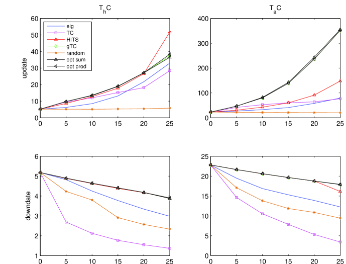
Fig. 2: Evolution of $T_{h}C$ and $T_{a}C$ for the network GD95b when 25 edge modifications are performed working on the matrix $A$ associated with the digraph: updates (top) and downdates (bottom).

The small network is used to compare the effectiveness of the proposed heuristics with a “brute force” approach where each virtual edge is added in turn and the change in total communicability is monitored in order to find the “optimal” choice. Since we are tracking not one but two quantities, $T_{h}C(A)$ and $T_{a}C(A)$, we monitor both $T_{h}C(A)+T_{a}C(A)$ and $T_{h}C(A)\cdot T_{a}C(A)$ and choose the optimal edge for either one of them. These methods are labeled as opt sum and opt prod, respectively. We perform a similar set of experiments for the downdating. As a baseline method, we also report results for a random selection of the edges in all our tests. The random methods are labeled as random or b:random, depending on whether we work on the matrix $A$ or on $\mathscr{A}$.

In Fig. 2 we show plots of the total communicabilities $T_{h}C$ and $T_{a}C$ when up to $K=25$ edge modifications are performed. We limit ourselves to the results for the heuristics based on the original digraph (matrix $A$). The results show that the heuristic gTC performs as well as the “optimal” choice based on brute force, while of course being much less expensive, in tackling both the updating and downdating problem. Note moreover that the performance of the methods HITS and gTC is different for this network. This result agrees with what one would expect, in view of the small gap $\sigma_{1}-\sigma_{2}$ of the adjacency matrix under study. When considering the problem of downdating, on the other hand, all the methods perform well. In particular we want to stress again the excellent performance of the method gTC. The only exception is perhaps the heuristic eig, whose performance for the first 5 steps is comparable with the random choice. This result confirms our claim that this heuristic, which was shown in [1] to work very well for undirected networks, is not a good approach in the directed case.

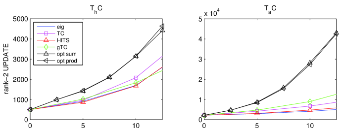
Fig. 3: Evolution of $T_{h}C$ and $T_{a}C$ for the network GD95b when 25 symmetric edge modifications are performed working on the matrix $A$ associated with the digraph. The optimal methods refer to the rank-one selection of the modifications

In Fig. 3 we display the evolution of the total communicability indices under rank-two updates. In this plot we retain the same names for the techniques as used in case of the rank-one modifications; however, the quantities used to derive the rankings are defined as in subsection 5.1. In this figure, each step corresponds to a rank-two symmetric modification, for the heuristic based on the edge centrality measures, and to two rank-one modifications, for the optimal methods. Thus, the plots for the optimal methods coincide with those in Fig. 2. The results displayed in Fig. 3 tell us that the symmetric rank-two modifications of the matrix may not lead to results as good as those obtained with the rank-one updates. Indeed, for both the total hub and authority communicabilities we have at least three methods in Fig. 2 that outperform all the methods used in Fig. 3. For this reason, we have not further investigate this approach.

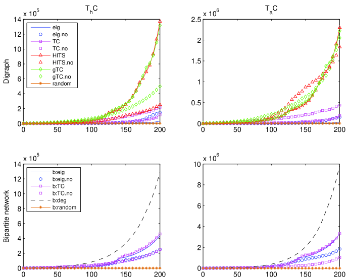
Fig. 4: Evolution of $T_{h}C$ and $T_{a}C$ for the network Computational Complexity when 200 updates are selected working on the matrix $A$ associated with the digraph (top) and on its bipartite version $\mathscr{A}$ (bottom).

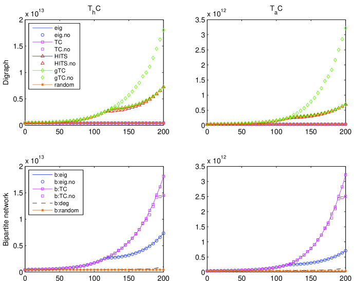
Fig. 5: Evolution of $T_{h}C$ and $T_{a}C$ for the network Abortion when 200 updates are selected working on the matrix $A$ associated with the digraph (top) or on its bipartite version $\mathscr{A}$ (bottom).

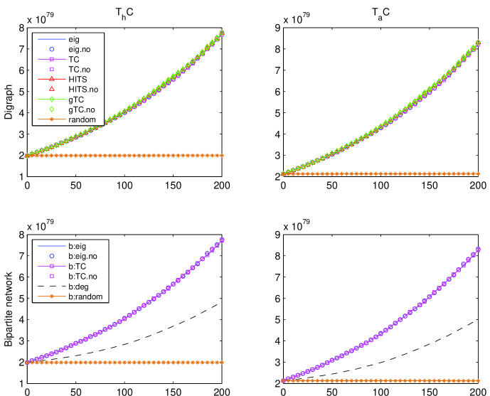
Fig. 6: Evolution of $T_{h}C$ and $T_{a}C$ for the network Twitter when 200 updates are selected working on the matrix $A$ associated with the digraph (top) and on its bipartite version $\mathscr{A}$ (bottom).

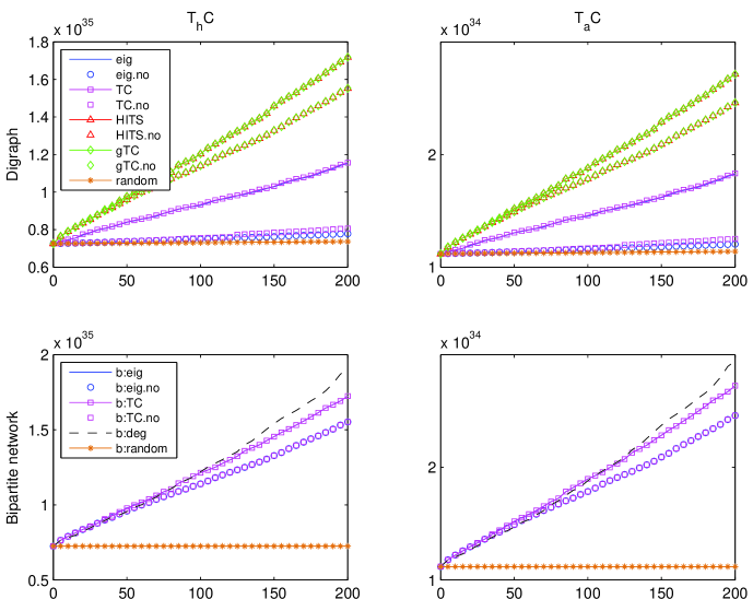
Fig. 7: Evolution of $T_{h}C$ and $T_{a}C$ for the network cit-HepTh when 200 updates are selected working on the matrix $A$ associated with the digraph (top) or on its bipartite version $\mathscr{A}$ (bottom).

The results on the small network give us confidence that at least some of our proposed heuristic do a very good job at enhancing the communicability properties of digraphs. In the remaining tests we concentrate on the larger four networks, for which the “optimal,” brute force approaches are not practical. All experiments were performed using MATLAB Version 8.0.0.783 (R2012b) on an IBM ThinkPad running Ubuntu 14.04 LTS, a 2.5 GHZ Intel Core i5 processor, and 3.7 GiB of RAM.

Figs. 4-7 display the evolution of the total hub and communicability centrality (rescaled by the number of edges in the network) when $K=200$ updates are selected using the criteria previously introduced. The plots at the top of each figure display the evolution of the total hub communicability (left) and total authority communicability (right) when the digraph is modified using the techniques developed for the directed case. The bottom plots show the evolution of the two indices obtained when the modifications are selected by working on $\mathscr{A}$. As expected, the proposed heuristics are dramatically better than the random choice.

The results show that the heuristics b:eig(.no) and b:TC(.no) perform similarly to HITS(.no) and gTC(.no). The methods eig(.no) and TC(.no) display erratic behavior and often perform very poorly, as shown in Figs. 4, 5, and 7. The method eig(.no) also suffers from the restriction that the dominant eigenvalue must be simple, which is not always true in practice. Likewise, the performance of b:deg is generally unsatisfactory, with the exception of $T_{a}C(A)$ for the network Computational Complexity where it outperforms the other techniques (see Fig. 4). Overall, considering also the timings (see Table 3), the best performance is displayed by the heuristics gTC(.no) and HITS(.no) and by their undirected counterparts b:TC(.no) and b:eig(.no). The only possible exception is the Computational Complexity network, for which the heuristics for the directed case outperform those for the undirected, bipartite counterpart.

The disagreement between the results for the heuristics labeled HITS and b:eig for the network Computational Complexity is at first sight puzzling. The two criteria should lead to the same edge selection and therefore to the same results, since the principal eigenvector of $\mathscr{A}$ is ${\bf q}_{1}=({\bf u}_{1}^{T},{\bf v}_{1}^{T})^{T}$ and thus $q_{1}(i)=u_{1}(i)$ and $q_{1}(j^{\prime})=v_{1}(j)$ in the definition of the heuristic b:eig. However, if at least two edges have the same centrality score when working with b:eig and HITS, then the two methods may select different edges. In this case, after the edge modification has been performed, the adjacency matrices manipulated by the two methods are different, thus causing the difference we observe in Fig. 4. The difference will be more pronounced if the tie between edges occur at the beginning of the modification process.

Table 3: Timings in seconds when $K=200$ updates are selected for the networks in our Dataset using the methods described.

	Computational
	Complexity	Abortion	Twitter	cit-HepTh
eig	12.51	53.27	139.82	217.12
eig.no	0.13	0.73	1.75	1.33
TC	114.67	62.22	187.22	163.55
TC.no	0.61	0.76	2.19	1.02
HITS	8.35	50.69	133.50	88.82
HITS.no	0.09	0.63	1.69	0.67
gTC	10.63	59.31	183.48	205.17
gTC.no	0.12	0.68	1.77	1.28
b:eig	9.35	52.43	134.03	99.70
b:eig.no	0.21	0.69	1.66	0.88
b:deg	11.00	85.06	256.66	84.95
b:TC	11.39	59.31	154.97	139.50
b:TC.no	0.11	0.72	1.67	0.82

Table 3 contains the timings (in seconds) employed for the selection of the $K=200$ virtual edges to be updated. The heuristics used were implemented using mostly built-in MATLAB functions, such as the function eigs used for computing the largest eigenvalue. For the heuristics requiring the computation of a matrix function times a vector we used the code funm_kryl by S. Güttel [17]. To implement the degree-based heuristic we wrote our own code, which is far from optimal when compared to the other ones. The relatively high timings reported for this heuristic can likely be reduced with a more careful implementation. When interpreting the results, it has to be kept in mind that the size $\tau$ of the set of virtual edges can be pretty large (cf. Table 2). We have observed that, for all the methods, roughly half of the reported computing time is spent in the computation of the products used in the definitions of the edge centrality measures. Nevertheless, the timings range from very small to moderate in all cases, showing the feasibility of the proposed heuristics.

Among all the methods we tested on directed networks for the updating problem, the best performance is displayed by HITS(.no), gTC(.no), b:eig(.no) and b:TC(.no) with the methods that manipulate $A$ having the edge when $\sigma_{1}-\sigma_{2}$ is small. Due to its erratic behavior, we cannot recommend the use of b:deg in general.

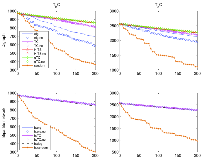
Fig. 8: Evolution of $T_{h}C$ and $T_{a}C$ for the network Computational Complexity when 200 downdates are selected working on the matrix $A$ associated with the digraph (top) and on its bipartite version $\mathscr{A}$ (bottom).

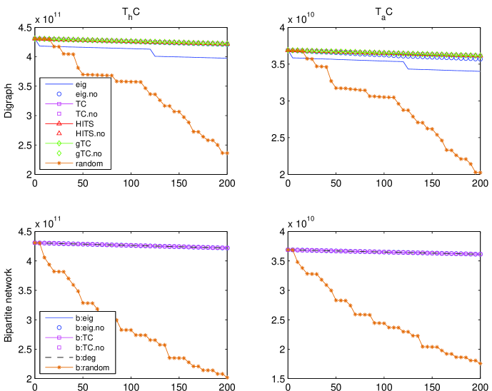
Fig. 9: Evolution of $T_{h}C$ and $T_{a}C$ for the network Abortion when 200 downdates are selected working on the matrix $A$ associated with the digraph (top) and on its bipartite version $\mathscr{A}$ (bottom).

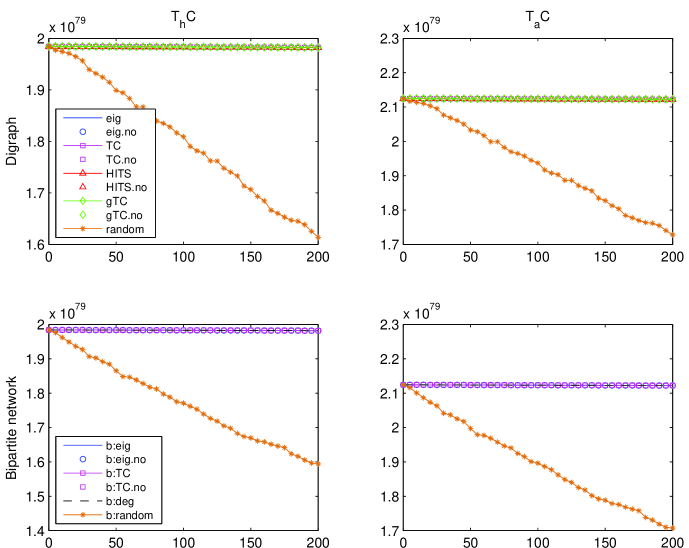
Fig. 10: Evolution of $T_{h}C$ and $T_{a}C$ for the network Twitter when 200 downdates are selected working on the matrix $A$ associated with the digraph (top) and on its bipartite version $\mathscr{A}$ (bottom).

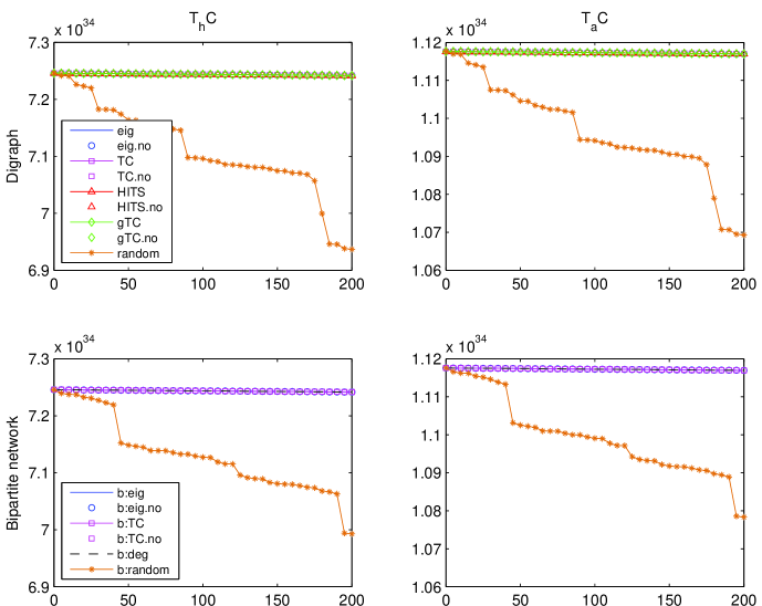
Fig. 11: Evolution of $T_{h}C$ and $T_{a}C$ for the network cit-HepTh when 200 downdates are selected working on the matrix $A$ associated with the digraph.

Table 4: Timings in seconds when $K=200$ downdates are selected for the networks in our Dataset using the methods described.

	Computational
	Complexity	Abortion	Twitter	cit-HepTh
eig	5.83	7.77	16.65	201.29
eig.no	0.04	0.04	0.05	1.03
TC	104.12	15.05	75.35	126.18
TC.no	0.92	0.07	0.39	0.73
HITS	2.72	4.71	13.32	63.40
HITS.no	0.02	0.02	0.08	0.34
gTC	5.49	12.06	60.77	175.02
gTC.no	0.04	0.08	0.29	0.80
b:eig	4.31	6.63	15.10	85.87
b:eig.no	0.03	0.04	0.05	1.89
b:deg	0.06	0.15	3.94	8.37
b:TC	5.51	11.66	39.02	126.44
b:TC.no	0.02	0.05	0.16	0.42

Similar conclusions can be drawn when considering the results for the downdating problem, although the differences among the techniques are less pronounced (Figs. 8–11 and Table 4). Indeed, the results shown confirm the effectiveness of the techniques based on the edge HITS and total communicability centralities and of their variants which do not require the recomputation of the rankings. As in the case of the updating problem, the results returned by these two methods essentially reproduce those obtained when working on $\mathscr{A}$ using the heuristics b:eig(.no) and b:TC(.no).

The methods eig(.no) and TC(.no) perform no better (and in some cases worse) than gTC(.no) and HITS(.no), while b:deg is usually outperformed by b:eig(.no) or b:TC(.no).

Concerning the timings, if we compare the results in Tables 3 and 4 we can see that the values in Table 3 are in general higher that those in Table 4. This is easily understood in view of what we observed before, if one compares the number of virtual edges $\tau$ with the number of edges $m$ in each network in the dataset (see Table 2).

While we do not provide a formal assessment of the computational cost of the various heuristics, arguments similar to those found in [1] indicate that the cost of the more efficient heuristics can be expected to scale approximately like ${\pazocal O}(n)$ or ${\pazocal O}(n\log n)$ with the number of nodes $n$.

In conclusion, by considering the overall performance of the methods and their cost (in terms of timings), we find that the best criteria for our updating/downdating goals are the methods HITS(.no) and gTC(.no). Besides these, satisfactory results may also be obtained using b:eig(.no) or b:TC(.no). From the timings in Tables 3 and 4 we can deduce that the heuristics HITS(.no) are in general slightly faster than b:eig(.no) and may thus be preferred. Concerning whether it is better to use gTC(.no) or b:TC(.no), we anticipate that the first will be preferrable when used in conjunction with fast algorithms for the approximation of bilinear forms involving generalized matrix functions.

7 Conclusions and future work

In this work we have extended the notion of total network communicability to directed graphs, and developed heuristics for manipulating an existing directed network so as to enhance its communicability properties. In doing so we made use of the concept of alternating walks, which allows us to take into account the dual role played by each node in a digraph, namely, receiver and broadcaster of information. This in turn led us in a natural way to the (rather overlooked) concept of generalized matrix function, first introduced in [18]. As shown in the paper, this concept allows one to express various communicability measures for digraphs in a compact form.

Our computational results indicate that the heuristics which take into account the dual role of nodes in directed networks tend to be preferable to those that do not. We also showed that these heuristics are very fast in practice.

Future work will address computational issues for large-scale networks (in particular, fast algorithms for estimating the row and column sums of generalized matrix functions). Another avenue for future work is the extension of the techniques in this paper and in [1] to weighted graphs. We also plan to investigate the use of our heuristics to tune other network properties. Preliminary tests suggest that our edge modification techniques are effective at increasing the synchronizability in directed graphs (see, e.g., [28]). A more systematic exploration of this application is left for future work.

References

- [1] F. Arrigo and M. Benzi, Updating and downdating techniques for optimizing network communicability, to appear in SIAM J. Sci. Comput.
- [2] M. Benzi, E. Estrada, and C. Klymko, Ranking hubs and authorities using matrix functions, Linear Algebra Appl. 438 (2013), pp. 2447–2474
- [3] M. Benzi and C. Klymko, Total communicability as a centrality measure, J. Complex Networks 1(2) (2013), pp. 124–149.
- [4] M. Benzi and C. Klymko, On the limiting behavior of parameter-dependent network centrality measures, SIAM J. Matrix Anal. Appl., 36 (2015), pp. 686–706.
- [5] P. Bonacich Power and centrality: A family of measures, Am. J. Sociol. 92 (1987) 92, pp. 1170-1182.
- [6] J. J. Crofts, E. Estrada, D. J. Higham, and A. Taylor, Mapping directed networks, Electron. Trans. Numer. Anal. 37 (2010), pp. 337–350.
- [7] T. Davis and Y. Hu, University of Florida sparse matrix collection, http://www.cise.ufl.edu/research/sparse/matrices/.
- [8] E. Estrada and N. Hatano, Statistical–mechanical approach to subgraph centrality in complex networks, Chem. Phys. Lett. 439 (2007), pp. 247–251.
- [9] E. Estrada and N. Hatano, Communicability in complex networks, Phys. Rev. E, 77 (2008), article 036111.
- [10] E. Estrada, N. Hatano, and M. Benzi, The physics of communicability in complex networks, Phys. Rep., 514 (2012), pp. 89–119.
- [11] E. Estrada and J. A. Rodríguez-Velázquez, Subgraph centrality in complex networks, Phys. Rev. E, 71 (2005), 056103.
- [12] A. Farahat, T. Lofaro, J. C. Miller, G. Rae, and L. A. Ward, Authority rankings from HITS, PageRank, and SALSA: existence, uniqueness, and effect of initialization, SIAM J. Sci. Comput., 27 (2006), pp. 1181–1201.
- [13] M. C. Gates and M. E. J. Woolhouse, Controlling infectious disease through the targeted manipulation of contact network structure, Epidemics, 12 (2015), pp. 11–19.
- [14] Gephi sample dataset, http://wiki.gephi.org/index.php/Datasets.
- [15] G. H. Golub and G. Meurant, Matrices, Moments and Quadrature with Applications, Princeton University Press, Princeton, 2010.
- [16] G. H. Golub and C. F. Van Loan, Matrix Computations. Fourth Edition, Johns Hopkins University Press, Baltimore and London, 2013.
- [17] S. Güttel, funm_kryl toolbox for Matlab, www.mathe.tu-freiberg.de/ guttels/funm_kryl/.
- [18] J. B. Hawkins and A. Ben–Israel, On generalized matrix functions, Linear and Multilinear Algebra 1(2) (1973), pp. 163–171.
- [19] N. J. Higham, Functions of Matrices. Theory and Computation, Society for Industrial and Applied Mathematics, Philadelphia, PA, 2008.
- [20] S. Hoory, N. Linial, and A. Wigderson, Expander graphs and their applications, Bull. Amer. Math. Soc., 43 (2006), pp. 439–561.
- [21] R. A. Horn and C. R. Johnson, Matrix Analysis. Second Edition, Cambridge University Press, 2013.
- [22] J. Kleinberg, Authoritative sources in a hyperlinked environment, J. ACM 46 (1999), pp. 604–632.
- [23] A. N. Langville and C. D. Meyer, Google’s PageRank and Beyond: The Science of Search Engine Rankings, Princeton University Press, Princeton, NJ, 2006.
- [24] H. Tong, B. Aditya Prakash, T. Eliassi–Rad, M. Faloutsos, and C. Faloutsos, Gelling, and melting, large graphs by edge manipulation, Proceedings of the 21st ACM international conference on information and knowledge management (2012), pp. 245–254.
- [25] P. Tsapras, Dataset for experiments on link analysis ranking algorithms, http://www.cs.toronto.edy/tsap/experiments/datasets/index.html/.
- [26] J. Wu, M. Barahona, Y. Tan, and H. Deng, Natural connectivity of complex networks, Chinese Physical Letters, 27 (2010), 078902.
- [27] J. Wu, M. Barahona, Y. Tan, and H. Deng, Robustness of random graphs based on graph spectra, Chaos, 22 (2012), 043101.
- [28] A. Zeng, L. Lü, and T. Zhou, Manipulating directed networks for better synchronization, New Journal of Physics, 14 (2012), 083006.