Ensemble Transport Adaptive Importance Sampling

Abstract

Markov chain Monte Carlo methods are a powerful and commonly used family of numerical methods for sampling from complex probability distributions. As applications of these methods increase in size and complexity, the need for efficient methods increases. In this paper, we present a particle ensemble algorithm. At each iteration, an importance sampling proposal distribution is formed using an ensemble of particles. A stratified sample is taken from this distribution and weighted under the posterior, a state-of-the-art ensemble transport resampling method is then used to create an evenly weighted sample ready for the next iteration. We demonstrate that this ensemble transport adaptive importance sampling (ETAIS) method outperforms MCMC methods with equivalent proposal distributions for low dimensional problems, and in fact shows better than linear improvements in convergence rates with respect to the number of ensemble members. We also introduce a new resampling strategy, multinomial transformation (MT), which while not as accurate as the ensemble transport resampler, is substantially less costly for large ensemble sizes, and can then be used in conjunction with ETAIS for complex problems. We also focus on how algorithmic parameters regarding the mixture proposal can be quickly tuned to optimise performance. In particular, we demonstrate this methodology’s superior sampling for multimodal problems, such as those arising from inference for mixture models, and for problems with expensive likelihoods requiring the solution of a differential equation, for which speed-ups of orders of magnitude are demonstrated. Likelihood evaluations of the ensemble could be computed in a distributed manner, suggesting that this methodology is a good candidate for parallel Bayesian computations.
Keywords: MCMC, importance sampling, Bayesian, inverse problems, ensemble, resampling.

1 Introduction

Having first been developed in the early 1970s[22], Markov chain Monte Carlo (MCMC) methods have been of increasing importance and interest in the last 20 years or so. They allow us to sample from complex probability distributions which we would not be able to sample from directly. In particular, these methods have revolutionised the way in which inverse problems can be tackled, allowing full posterior sampling when using a Bayesian framework.

However, this often comes at a very high cost, with a very large number of iterations required in order for the empirical approximation of the posterior to be considered good enough. As the cost of computing likelihoods can be extremely large, this means that many problems of interest are simply computationally intractable.

This problem has been tackled in a variety of different ways. One approach is to construct increasingly complex MCMC methods which are able to use the structure of the posterior to make more intelligent proposals, leading to more thorough exploration of the posterior with fewer iterations. For example, the Hamiltonian or Hybrid Monte Carlo (HMC) algorithm uses gradient information and symplectic integrators in order to make very large moves in state with relatively high acceptance probabilities[43]. Non-reversible methods are also becoming quite popular as they can improve mixing[3]. Riemann manifold Monte Carlo methods exploit the Riemann geometry of the parameter space, and are able to take advantage of the local structure of the target density to produce more efficient MCMC proposals[20]. This methodology has been successfully applied to MALA-type proposals and methods which exploit even higher order gradient information[6].

Since the clock speed of an individual processor is no longer following Moore’s law[32], improvements in computational power are largely coming from the parallelisation of multiple cores. As such, the area of parallel MCMC methods is becoming increasingly of interest. One class of parallel MCMC method uses multiple proposals, with only one of these proposals being accepted. Examples of this approach include multiple try MCMC[27] and ensemble MCMC[33]. In [7], a general construction for the parallelisation of MCMC methods was presented, which demonstrated speed ups of up to two orders of magnitude when compared with serial methods on a single core. Another approach involves pre-fetching, where the possible future acceptances/rejections are calculated in advance[2].

A variety of other methods have been designed with particular scenarios in mind. For instance, sampling from high/infinite-dimensional posterior distributions is of interest in many applications. The majority of Metropolis-Hastings algorithms suffer from the curse of dimensionality, requiring more samples for a given degree of accuracy as the parameter dimension is increased. However some dimension-independent methods have been developed, based on Crank-Nicolson discretisations of certain stochastic differential equations[14]. Other ideas such as chain adaptation[21] and early rejection of samples can also aid reduction of the computational workload[45].

However, high dimensionality is not the only challenge that we may face. Complex structure in low dimensions can cause significant issues. These issues may arise due to large correlations between parameters in the posterior, leading to long thin curved structures which many standard methods can struggle with. These features are common, for example, in inverse problems related to epidemiology and other biological applications[23].

Multimodality of the posterior can also lead to incredibly slow convergence in many methods. Many methods allow for good exploration of the current mode, but the waiting time to the next switch of the chain to another mode may be large. Since many switches are required in order for the correct weighting to be given to each mode, and for all of the modes to be explored fully, this presents a significant challenge. One application where this is an ever-present problem is that of mixture models. Given a dataset, where we know that the data is from two or more different distributions, we wish to be able to identify the parameters, e.g. the mean and variance and relative weight, of each part of the mixture[29]. The resulting posterior distribution is invariably a multimodal distribution, since the likelihood is invariant to permutations. Metropolis-Hastings algorithms, for example, will often fail to converge in a reasonable time frame for problems such as this. Since the posterior may be multimodal, independent of this label switching, it is important to be able to efficiently sample from the whole posterior.

Importance samplers are another class of methods which allow us to sample from complex probability distributions. A related class of algorithms, adaptive importance sampling (AIS) [26] reviewed in[5], had received less attention until their practical applicability was demonstrated in the mid-2000s[11, 9, 24, 4]. AIS methods produce a sequence of approximating distributions, constructed from mixtures of standard distributions, from which samples can be easily drawn. At each iteration the samples are weighted, often using standard importance sampling methods. The weighted samples are used to train the adapting sequence of distributions so that samples are drawn more efficiently as the iterations progress. The weighted samples form a sample from the posterior distribution under some mild conditions [37, 30].

Ensemble importance sampling schemes also exist, e.g. population Monte Carlo (PMC) [10]. PMC uses an ensemble to build a mixture or kernel density estimate (KDE) of the posterior distribution. The efficiency of this optimisation is restricted by the component kernel(s) chosen, and the quality of the current sample from the posterior[8, 15, 16]. Extensions, such as layered adaptive importance sampling[31], adaptive multiple importance sampling algorithm (AMIS) [12], and adaptive population importance sampling (APIS) [30] have enabled these methods to be applied to various applications, including population genetics [44].

In this paper, we present a framework for ensemble importance sampling, which can be built around many of the current Metropolis-based methodologies in order to create an efficient target distribution from the current ensemble. The method makes use of a resampler based on optimal transport which has been used in the context of particle filters[36]. We also detail how algorithmic parameters can be quickly tuned into optimal regimes, with respect to the effective sample size statistic. In particular we demonstrate the advantages of this method when attempting to sample from multimodal posterior distributions, such as those arising from inference for mixture models. The method that we present is specifically designed to tackle the challenges of certain types of low-dimensional inverse problem which have complex posterior structure, for example multimodality or strong correlations, and expensive likelihood evaluations. We will demonstrate that this methodology allows us to sample from such a posterior distribution with greater precision per likelihood evaluation than standard MCMC chains of the same type.

The method considered is similar to population Monte Carlo methods which have been previously studied, for example in [18]. However our approach exploits the current state-of-the-art resamplers, and adaptively optimises algorithmic parameters. Higher accuracy resamplers, that provide a deterministic resample which optimally reflects the statistics of the original sample, lead to better mixture approximations of the posterior. These approximations can then be used to construct stable and efficient importance sampling proposals. The cost of the state-of-art resamplers can be prohibitive for large ensemble sizes, which are necessary for sampling in moderately higher dimensions, and as such we also present a greedy approximation of the optimal transport resampler, which provides us with good results for a fraction of the cost. We also detail how scaling parameters in the MCMC proposals can be quickly tuned, leading us to an efficient and fully-automated algorithm. We will demonstrate that despite additional overheads, the ETAIS methodology can outperform its plain Metropolis-Hastings cousin by orders of magnitude to reach a histogram of a particular degree of convergence.

In Section 2 we introduce some mathematical preliminaries upon which we will later rely. In Section 3 we present the general framework of the ETAIS algorithm. In Section 4 we consider adaptive versions of ETAIS which automatically tune algorithmic parameters concerned with the proposal distributions. In Section 5 we introduce the multinomial transformation (MT) algorithm which is a less accurate but faster alternative to resamplers which solve the optimal transport problem exactly. In Section 6 we consider consistency of the ETAIS algorithm. In Section 7 we briefly look at one particular advantageous property of this approach. In Section 8 we present some numerical examples, before a brief conclusion and discussion in Section 9.

2 Preliminaries

In this Section we will introduce preliminary topics and algorithms that will be referred to throughout the paper.

2.1 Bayesian inverse problems

In this paper, we focus on the use of MCMC methods for characterising posterior probability distributions arising from Bayesian inverse problems. We wish to learn about a particular unknown quantity $x$, of which we are able to make direct or indirect noisy observations. For now we say that $x$ is a member of a Hilbert space $X$.

The quantity $x$ is mapped on to observable space by the observation operator $\mathcal{G}:X\to\mathbb{R}^{d}$. We assume that the observations, $D$, are subject to Gaussian noise,

$$D=\mathcal{G}(x)+\varepsilon,\qquad\varepsilon\sim\mathcal{N}(0,\Sigma).$$ (1)

These modelling assumptions allow us to construct the likelihood of observing the data $D$ given the quantity $x=x^{*}$. Rearranging (1) and using the distribution of $\varepsilon$, we get:

$$\mathbb{P}(D|x=x^{*})\propto\exp\left(-\frac{1}{2}\|\mathcal{G}(x^{*})-D\|_{\Sigma}^{2}\right)=\exp\left(-\Phi(x^{*})\right),$$ (2)

where $\|y_{1}-y_{2}\|^{2}_{\Sigma}=(y_{1}-y_{2})^{\top}\Sigma^{-1}(y_{1}-y_{2})$ for $y_{1},y_{2}\in\mathbb{R}^{d}$.

Then, according to Bayes’ theorem, the posterior density that we are interested in characterising is given, up to a constant of proportionality, by

$$\pi\propto\exp\left(-\Phi(x^{*})\right)\pi_{0}(x^{*}),$$

where $\pi_{0}$ is the prior density on the quantity of interest $x^{*}$.

2.2 Particle filters and resamplers

In this subsection we briefly review particle filters, since the development of the resampler that we incorporate into the ETAIS is motivated by this area. Particle filters are a class of Monte Carlo algorithm designed to solve the filtering problem. That is, to find the best estimate of the true state of a system when given only noisy observations of the system. The solution of this problem has been of importance since the middle of the 20th century in fields such as molecular biology, computational physics and signal processing. In recent years the data assimilation community has contributed several efficient particle filters, including the ensemble Kalman filter (EnKF) [19] and the ensemble transform particle filter (ETPF) [36].

The ETPF defines a coupling $T$ between two random variables $Y$ and $X$, allowing us to use the induced map as a resampler. An optimal coupling $T^{*}$ is one which maximises the correlation between $X$ and $Y$ [13]. This coupling is the solution to a linear programming problem in $M^{2}$ variables with $2M-1$ constraints, where $M$ is the size of the sample. Maximising the correlation preserves the statistics of $X$ in the new sample.

In this work we use the resampler used within these particle filters. We approximate the posterior density $\pi$, with an ensemble of weighted samples, $\{(w_{i},y_{i})\}_{i=1}^{M}$. In filtering problems the weights would be found by incorporating new observed data whereas here we simply use importance weights. These weighted samples can then be resampled, using the ETPF or otherwise, into a set of new equally-weighted samples $\{x_{i}\}_{i=1}^{M}$, such that

$$\sum\limits_{i=1}^{M}\!w_{i}\delta_{y_{i}}(\cdot)\quad\xrightarrow{\text{ETPF}}\quad\sum\limits_{i=1}^{M}\!\frac{1}{M}\delta_{x_{i}}(\cdot),$$ (3)

where $\delta_{x}(\cdot)$ is the Dirac delta measure.

The resamplers used within particle filters such as the ETPF are well suited to this problem since it is easy to introduce conditions in the resampling to ensure you obtain the behaviour you require. One downside is that the required ensemble size increases quickly with dimension, making it difficult to use in high-dimensional problems.

2.3 Deficiencies of Metropolis-type MCMC schemes

All MCMC methods are naively parallelisable. One can take a method and simply implement it multiple times over an ensemble of processors. All of the states of all of the ensemble member can be recorded, and in the time that it takes one MCMC chain to draw $N$ samples, $M$ ensemble members can draw $NM$ samples.

However, we argue that this is not an optimal scenario. First of all, unless we have a lot of information about the posterior, we will initialise the algorithm’s initial state in the tails of the distribution. The samples that are initially made as the algorithm finds its way to the mode(s) of the distribution cannot be considered to be samples from the target distribution, and must be thrown away. This process is known as the burn-in. In a naively parallelised scenario, each ensemble member must perform this process independently, and therefore mass parallelisation makes no inroads to cutting this cost.

Moreover, many MCMC algorithms suffer from poor mixing, especially in multimodal systems. The number of samples that it takes for an MCMC trajectory to switch between modes can be large, and given that a large number of switches are required before we have a good idea of the relative probability densities of these different regions, it can be prohibitively expensive.

Another aspect of Metropolis-type samplers is that information computed about a proposed state is simply lost if we choose to reject that proposal in the Metropolis step. An advantage of importance samplers is that no evaluations of $\mathcal{G}$ are ever wasted since all samples are saved along with their relative weighting.

These deficiencies of MCMC methods motivated the development of the Ensemble Transport Adaptive Importance Sampler (ETAIS). In the next section we will introduce the method in its most general form.

3 The Ensemble Transform Adaptive Importance Sampler (ETAIS)

Importance sampling can be a very efficient method for sampling from a probability distribution. A proposal density is chosen, from which we can draw samples. Each sample is assigned a weight given by the ratio of the target density and the proposal density at that point. They are efficient when the proposal density is concentrated in similar areas to the target density, and incredibly inefficient when this is not the case. The aim of the ETAIS is to use an ensemble of states to construct a proposal distribution which will be as close as possible to the target density. If this ensemble is large enough, the distribution of states will be approximately representative of the target density.

The proposal distribution could be constructed in many different ways, but we choose to use a mixture distribution, made up of a sum of MCMC proposal kernels e.g. Gaussians centred at the current state, as in RWMH. Once the proposal is constructed, we can sample a new ensemble from the proposal distribution, and each is assigned a weight given by the ratio of the target density and the proposal mixture density. Assuming that our proposal distribution is a good one, then the variance of the weights will be small, and we will have many useful samples. Finally, we need to create a set of evenly weighted samples which best represent this set of weighted samples. This is achieved by implementing a resampling algorithm. These samples are not stored in order to characterise the posterior density, since the resampling process is not exact. They are simply needed in order to inform the mixture proposal distribution for the next iteration of the algorithm.

Initially we will use the ETPF resampler algorithm[36], although we will suggest an alternative strategy in Section 5, for examples where a large ensemble is required, and for which the ETPF may become more expensive. The resampling algorithm gives us a set of evenly weighted samples which represents the target distribution well, which we can use to iterate the process again. The algorithm is summarised in Algorithm 1.

The choice of resampling algorithm is important since its output is used to formulate the proposal distribution for the next iteration. A basic resampler may be cheap to implement, but the resulting sample, and in turn the next iteration’s proposal distribution, may not be as representative of the target distribution. This leads to higher variances of the weights in the importance sampler, and therefore to slower convergence to the target density.

We wish to sample states $x\in X$ from a posterior probability distribution with density $\pi$. Since we have $M$ ensemble members, we represent the current state of all of the Markov chains as a vector ${\mathbf{X}}=[x_{1},x_{2},\ldots,x_{M}]^{\top}$. We are also given a transition kernel $\nu(\cdot,\cdot)$, which might come from an MCMC method, for example the random walk Metropolis-Hastings proposal density $\nu(\cdot,x)\sim\mathcal{N}(x,\beta^{2})$, where $\beta^{2}\in\mathbb{R}$ defines the variance of the proposal.

1 Set ${\mathbf{X}}^{(0)}={\mathbf{X}}_{0}=[x_{1}^{(0)},x_{2}^{(0)},\ldots,x_{M}^{(0)}]^{\top}$.

2 for $i=1,\dots,N$ do

3       Sample ${\mathbf{Y}}^{(i)}=[y_{1}^{(i)},y_{2}^{(i)},\ldots,y_{M}^{(i)}]^{\top},\quad y_{j}^{(i)}\sim\nu(\cdot;x_{j}^{(i-1)})$.

4       Calculate ${\mathbf{W}}^{(i)}=[w_{1}^{(i)},w_{2}^{(i)},\ldots,w_{M}^{(i)}]^{\top},$  $w^{(i)}_{j}=\frac{\pi(y_{j}^{(i)})}{\chi(y_{j}^{(i)};{\mathbf{X}}^{(i-1)})}$, where

$$\chi(\cdot;{\mathbf{X}}^{(i-1)})=\frac{1}{M}\sum_{j=1}^{M}\nu(\cdot;x_{j}^{(i-1)}).$$

5      Resample: $({\mathbf{W}}^{(i)},{\mathbf{Y}}^{(i)})\rightarrow(\frac{1}{M}\mathbf{1},{\mathbf{X}}^{(i)})$.

6      

7Output $({\mathbf{W}},{\mathbf{Y}})$.

Algorithm 1 The ensemble transform adaptive importance sampler (ETAIS).

Since the resampling does not give us a statistically identical sample to that which is input, we cannot assume that the samples ${\mathbf{X}}^{(i)}$ are samples from the posterior. Therefore, as with serial importance samplers, the weighted samples $({\mathbf{W}},{\mathbf{Y}})_{i=1}^{N}$ are the samples from the posterior that we will analyse.

In each iteration of the algorithm, we are required to compute the likelihood for each member of the ensemble. In the case where the likelihood is expensive to compute, for example because it requires the numerical approximation of an ODE or PDE, and/or there is a very large amount of observations in the data, it will be expedient to split this computational effort across multiple cores. Whether this is efficient will depend on the architecture of the machine, and the relative cost of communication across the cores, to the cost of the likelihood evaluation. Evaluation of the denominator in the weights also contributes to the overhead costs of this approach over and above a standard MCMC method, but this too can be parallelised efficiently, depending on communication costs of the architecture of the machine, reducing the $\mathcal{O}(M^{2})$ cost to $\mathcal{O}(M)$ over $M$ cores, for example.

The key is to choose a suitable transition kernel $\nu$ such that if $\mathbf{X}^{(i)}$ is a representative sample of the posterior, then the mixture density $\chi(\cdot;{\mathbf{X}}^{(i)})$ is a good approximation of the posterior distribution. If this is the case, the newly proposed states ${\mathbf{Y}}^{(i)}$ will also be a good sample of the posterior with low variance in the weights ${\mathbf{W}}^{(i)}$.

In Section 8, we will demonstrate how the algorithm performs, primarily using random walk (RW) proposals. We do not claim that this choice is optimal, but is simply chosen as an example to show that sharing information across ensemble members can improve on the original MH algorithm and lead to tolerances being achieved in fewer evaluations of $\mathcal{G}$. This is important since if the inverse problem being tackled involves computing the likelihood from a very large data set, or where the likelihood requires the numerical solution of a differential equation, this could lead to a large saving of computational cost. We have observed that using more complex (and hence more expensive) kernels $\nu$, does not significantly improve the speed of convergence of the algorithm for posteriors that we have considered, although kernels such as those used in MALA can be more stable for certain problems[42].

Care needs to be taken when choosing kernel(s) for the proposal distribution to ensure that the overall mixture is absolutely continuous with respect to the posterior distribution. For example, in many inverse problems we may be looking to find the value of certain physical parameters which may be strictly positive, or even bounded on an interval. In this case, proposal kernels $\nu$ should be picked which have the same support as the target. We will see an example of an unknown parameter being bounded in Section 8.3, where $\beta$-distributed proposals are made to ensure that the distribution is supported on $[0,1]$.

It is also possible, especially during the early stages of the algorithm, where the mixture proposal is a poor approximation of the target distribution, for a sample to be produced with a weight which is orders of magnitude bigger than the rest. This is a problem, since the resampling step will then lead to a vector of samples all centred at the outlier sample. Fortunately these spikes in weights can easily be detected, and in such a case, the sample for this iteration can be removed. The ETPF can then be used to formulate a new mixture sample with one sample placed at the outlier point, and the others distributed according to the sample positions before the problematic iteration. This ensures that the region where the problem occurred is better represented by the mixture, and prevents further spikes in this region.

4 Automated tuning of algorithm parameters

Efficient selection of scaling parameters in MCMC algorithms is critical to achieving optimal mixing rates and hence achieving fast convergence to the target density. It is well known that a scaling parameter which is either too large or too small results in a Markov chain with high autocorrelation. One aspect worthy of consideration with the ETAIS, is finding an appropriate proposal kernel $\nu$ such that the mixture distribution $\chi$ is a close approximation to the posterior density $\pi$.

Most MCMC proposals have parametric dependence which allows the user to control their variance. For example, in the RW proposal $y=x+\beta\eta$, the parameter $\beta$ is the standard deviation of the proposal distribution. Therefore the proposal distributions can be tuned such that they are slightly over-dispersed. This tuning can take place during the burn-in phase of the algorithm. Algorithms which use this method to find optimal proposal distributions are known as adaptive MCMC algorithms, and have been shown to be convergent provided that they satisfy certain conditions[40, 41]. Alternatively, a costly trial and error scheme with short runs of the MCMC algorithm can be used to find an acceptable value of $\beta$.

Algorithms which use mixture proposals, e.g. ETAIS, must tune the variance of the individual kernels within the proposal mixture. This adaptivity during early iterations has some added benefits over and above finding an optimal parameter regime for the algorithm. If the initial value of the proposal variance is chosen to be very large, then the early mode-finding stages of the algorithm are expedited. Adaptively reducing the proposal variances to an optimal value then allows us to explore each region efficiently. Using an ensemble of chains allows quick and effective assessment of the value of the optimal scaling parameter.

In many MCMC algorithms such as the Random Walk Metropolis-Hastings (RWMH) algorithm, the optimal scaling parameter can be found by searching for the parameter value which gives an optimal acceptance rate, e.g. for near Gaussian targets the optimal rates are 23.4% for RWMH and 57.4% for MALA[39]. This method is not applicable to ETAIS so we must use other statistics to optimise the scaling parameter. Section 4.1 gives some possible methods for tuning $\beta$.

4.1 Statistics for Determining the Optimal Scaling Parameter

4.1.1 Determining optimal scaling parameter using error analysis

When available, an analytic form for the target distribution allows us to assess the convergence of sampling algorithms to the target distribution. Common metrics for this task include the relative error between the sample moments and the target’s moments, or the relative $L^{2}$ error between the sample histogram and the target density, $\pi(x|D)$. The relative error in the $n$-th moment, $\hat{m}_{n}$, is given by:

$$e=\left|\frac{\hat{m}_{n}-\mathbb{E}[X^{n}]}{\mathbb{E}[X^{n}]}\right|,\quad\text{where}\quad\hat{m}_{n}=\frac{1}{N}\sum_{i=1}^{N}\!x_{i}^{n},$$ (4)

and $\{x_{i}\}_{i=1}^{N}$ is a sample of size $N$.

The relative $L^{2}$ error, $E$, between a continuous density function to a piecewise constant approximation of that density, can be defined by considering the difference in mass between the self-normalised histogram of the samples and the posterior distribution over a set of disjoint sets or “bins”:

$$E^{2}=\sum\limits_{i=1}^{n_{b}}\left[\displaystyle\int_{R_{i}}\!\pi(s|D)\,\mbox{d}s-vB_{i}\right]^{2}\Big{/}\sum\limits_{i=1}^{n_{b}}\left[\displaystyle\int_{R_{i}}\!\pi(s|D)\,\mbox{d}s\right]^{2},$$ (5)

where the regions $\{R_{i}\}_{i=1}^{n_{b}}$ are the $d$-dimensional histogram bins, so that $\bigcup_{i}R_{i}\subseteq X$ and $R_{i}\cap R_{j}=\emptyset$, $n_{b}$ is the number of bins, $v$ is the volume of each bin, and $B_{i}$ is the value of the $i$th bin. This metric converges to the standard definition of the relative $L^{2}$ error as $v\rightarrow 0$.

These statistics cannot be used in general to find optimal values of $\beta$ since they require the analytic solution, and are expensive to approximate. However they can be used to assess the ability of other indicators to find the optimal scaling parameters in a controlled setting.

4.1.2 The effective sample size

The effective sample size, $n_{\text{eff}}$, can be used to assess the efficiency of importance samplers. Ideally, in each iteration, we would like all $M$ of our samples to provide us with new information about the posterior distribution. In practice, we cannot achieve a perfect effective sample size of $M$.

The effective sample size of a weighted sample is defined in the following way:

$$n_{\text{eff}}=\frac{\left(\sum_{i=1}^{M}\!w_{i}\right)^{2}}{\sum_{i=1}^{M}\!w_{i}^{2}}\approx\frac{M{\mathbb{E}}(w)^{2}}{{\mathbb{E}}(w^{2})}=M\left(1-\frac{\mbox{var}(w)}{\mathbb{E}(w^{2})}\right).$$

The second two expressions are true when $M\rightarrow\infty$. From the last expression, if the variance of the weights is zero then $n_{\text{eff}}=M$; this is our ideal scenario. In the limit $M\rightarrow\infty$, maximising the effective sample size is equivalent to minimising the variance of the weights.

The statistic $n_{\text{eff}}$ is easier to deal with than the variance of the weights, as it takes values on $[1,M]$ while the variance of the weights takes values on $\mathbb{R}^{+}$. Moreover the variance of the weights can vary over many orders of magnitude causing numerical instabilities, so that the effective sample size is more desirable as an indicator of optimality.

In this paper we tune our simulations using the effective sample size statistic. We calculate this statistic using a sample size of $Mn_{k}$, where $1\leq n_{k}\leq N$ is sufficiently large enough to obtain a reasonable estimate of $n_{\text{eff}}$ with scaling parameter $\delta_{k}$. Calculating $n_{\text{eff}}$ over these subsets of the simulations tends to underestimate the optimal value of the scaling parameter due to the possibility of missing unlikely proposals with extreme weights.

The effective sample size also has another useful property; if we consider the algorithm in the early stages, for example, we have all $M$ samples in the tails of the target searching for a mode. The sample closest to the mode will have an exponentially higher weight and the effective sample size will be close to 1. In later stages the ensemble populates high density regions, and better represents the posterior distribution. This leads to smaller variation in the weights, and a higher effective sample size. By looking for approximations of the effective sample size which look like a stationary distribution, we can tell when the algorithm is working efficiently.

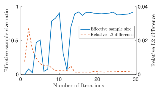
Figure 1: The effective sample size ratio and relative $L^{2}$ difference $E$ during the first 30 iterations. These numerics are taken from the example in Section 8.3.3 using the ETAIS-RW algorithm.

Figure 1 demonstrates that the effective sample size flattens out as the relative $L^{2}$ difference between the posterior distribution and the proposal distribution stabilises close to its minimum.

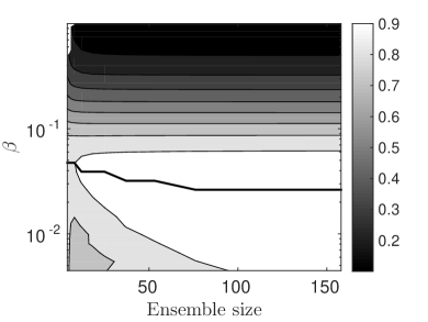
(a) Contours showing optimal ranges of the scaling parameter.

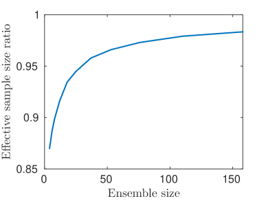
(b) The highest effective sample size achieved for each ensemble size.

Figure 2: The behaviour of the effective sample size as the ensemble size increases, considering the example in Section 8.1 using the ETAIS-RW algorithm.

Figure 2 shows how the effective sample size used in ETAIS is affected by the ensemble size. We see from subfigure (a) that as the ensemble size increases, the optimal scaling parameter decreases. This is expected since the larger ensemble allows for finer resolution in the proposal distribution approximation of the posterior distribution. We also see that the algorithm becomes less sensitive to changes in the scaling parameter as the ensemble size increases. Subfigure (b) shows that as the ensemble size increases, the algorithm becomes more efficient.

4.2 Adaptively Tuned ETAIS

To adapt the scaling parameter $\beta$, we use a version of the gradient ascent method modified for a stochastic function. Some more sophisticated examples are described in [41, 25, 1].

1 Define update times $\{n_{k}\}_{k}$.

2 for $n=1,\dots,N$ do

3       Complete steps 1-1 of Algorithm 1.

4       if $n\in\{n_{k}\}$ then

5             Divide ensemble into two halves. Use these halves to estimate the gradient in $n_{\text{eff}}$ at $\beta_{k}$.

6             Update $\beta_{k}$ using gradient ascent,

$$\beta_{k+1}=\beta_{k}+\gamma\nabla n_{\text{eff}}.$$

7      

Algorithm 2 Adaptively tuned ETAIS algorithm.

Our adaptive algorithm is given in Algorithm 2. We choose update times which, as suggested in Section 4.1.2 allow for a reasonable estimate of the effective sample size, but do not waste too many iterations. In Step 6, the gradient ascent parameter $\gamma$ may decrease over time, e.g. as a function of $n_{k}$.

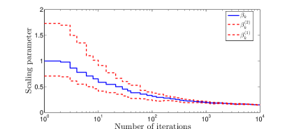
(a) AETAIS-RW algorithm adapting variance.

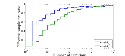
(b) AETAIS-RW algorithm maximising ESS.

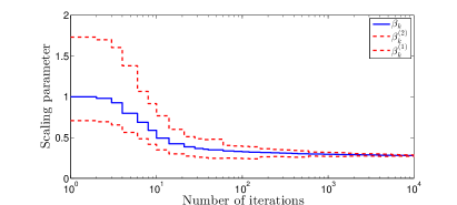
(c) AETAIS-MALA algorithm adapting variance.

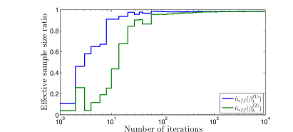
(d) AETAIS-MALA algorithm maximising ESS.

Figure 3: Demonstration of the convergence of the adaptive scaling parameter in the adaptively tuned ETAIS algorithms.

In the context of an expensive likelihood evaluation, slow convergence of the algorithmic parameters in this adaptive regime would be a concern. However, this is rarely an issue, due in part to the speed at which the ETAIS algorithm completes the burn-in phase. Figure 3 demonstrates this for two different versions of the ETAIS methodology with a RW proposal and a MALA[38] proposal. This picture is typical in our experience, with the scaling parameters converging in $\mathcal{O}(10^{2})$ iterations to an optimal regime.

5 Multinomial Transformation

Although the ETPF produces the optimal linear coupling, it can also become quite costly as the number of ensemble members is increased. It is arguable that in the context of ETAIS, we do not require this degree of accuracy, and that a faster more approximate method for resampling could be employed. One approach would be to use the bootstrap resampler, which simply takes the $M$ ensemble members’ weights and constructs a multinomial distribution, from which $M$ samples are drawn. This is essentially the cheapest resampling algorithm that one could construct. However it too has some drawbacks. The algorithm is random, and as such it is possible for all of the ensemble members in a particular region not to be sampled. This could be particularly problematic when attempting to sample from a multimodal distribution, where it might take a long time to find one of the modes again. The bootstrap filter is also not guaranteed to preserve the mean of the weighted sample, unlike the ETPF.

Ideally, we would like to use a resampling algorithm which is not prohibitively costly for moderately or large sized ensembles, which preserves the mean of the samples, and which makes it much harder for the new samples to forget a significant region in the density. This motivates the following algorithm, which we refer to as the multinomial transformation (MT), which is a greedy approximation of the ETPF resampler.

Instead of sampling $M$ times from an $M$-dimensional multinomial distribution as is the case with the bootstrap algorithm, we sample once each from $M$ different multinomials. Suppose that we have $M$ samples $y_{n}$ with weights $w_{n}$. The multinomial sampled from in the bootstrap filter has a vector of probabilities given by:

$$\frac{1}{\sum w_{n}}[w_{1},w_{2},\ldots,w_{M}]=\bar{\bf w},$$

with associated states $y_{n}$. We wish to find $M$ vectors $\{{\bf p}_{1},{\bf p}_{2},\ldots,{\bf p}_{M}\}\subset\mathbb{R}^{M}_{\geq 0}$ such that $\frac{1}{M}\sum{\bf p}_{i}=\bar{\bf w}$. The MT is then given by a sample from each of the multinomials defined by the vectors ${\bf p}_{i}=[p_{i,1},p_{i,2},\ldots,p_{i,M}]$ with associated states ${\bf y}_{i}$. Alternatively, as with the ETPF, a deterministic sample can be chosen by picking each sample to be equal to the mean value of each of these multinomial distributions, i.e. each new sample $\hat{x}_{i}$ is given by:

$$\hat{x}_{i}=\sum p_{i,j}x_{j},\qquad i\in\{1,2,\ldots,M\}.$$ (6)

The resulting sample has several properties which are advantageous in the context of being used with the ETAIS algorithm. Firstly, we have effectively chopped up the multinomial distribution used in the bootstrap filter into $M$ pieces, and we can guarantee that exactly one sample will be taken from each section. This leads to a much smaller chance of losing entire modes in the density, if each of the sub-multinomials is picked in an appropriate fashion. Secondly, if we do not make a random sample for each multinomial with probability vector $\bf p_{i}$ but instead take the mean of the multinomial to be the sample, this algorithm preserves the mean of the sample exactly. Lastly, as we will see shortly, this algorithm is significantly less computationally intensive than the ETPF.

There are of course infinitely many different ways that one could use to split the original multinomial up into $M$ parts, some of which will be far from optimal. The method that we have chosen is loosely based on the idea of optimal transport. We search out states with the largest weights, and choose a cluster around these points based on the closest states geographically. This method is not optimal since once most of the clusters have been selected the remaining states may be spread across the parameter space.

1 ${\bf z}=M\bar{{\bf w}}$.

2 for $i=1,\dots,M$ do

3       $J=\operatorname*{arg\,max}_{j}z_{j}$.

4       $p_{i,J}=\min\{1,z_{J}\}$.

5       $z_{J}=z_{J}-p_{i,J}$.

6       while $\sum_{j}p_{i,j}<1$ do

7             $K=\operatorname*{arg\,min}_{k\in\{k|z_{k}>0\}}\|y_{J}-y_{k}\|$.

8             $p_{i,K}=\min\{1-\sum_{j}p_{i,j},z_{K}\}$.

9             $z_{K}=z_{K}-p_{i,K}$.

10            

11      $x_{i}=\sum_{k}p_{i,k}y_{k}$.

12      

Algorithm 3 The multinomial transformation (MT).

Algorithm 3 describes the basis of the algorithm with deterministic resampling, using the means of each of the sub-multinomials as the new samples. This resampler was designed with the aims of being numerically cheaper than the ETPF, and more accurate than straight multinomial resampling. Therefore we now present numerical examples which demonstrate this.

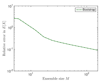
(a) Relative error in $\mathbb{E}(X)$

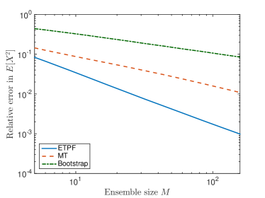
(b) Relative error in $\mathbb{E}(X^{2})$

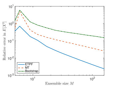
(c) Relative error in $\mathbb{E}(X^{3})$

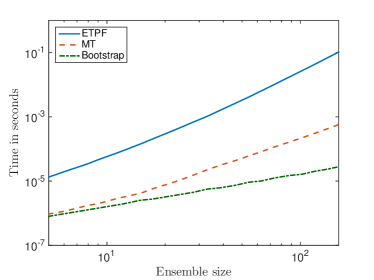
(d) Cost of resamplers per iteration

Figure 4: Comparison of the performance between different resampling schemes. The example in Section 8.1 is implemented for this demonstration.

To test the accuracy and speed of the three resamplers (ETPF, bootstrap and MT), we drew a sample of size $M$ from the proposal distribution $\mathcal{N}(1,2)$. Importance weights were assigned, based on a target distribution of $\mathcal{N}(2,3)$. The statistics of the resampled outputs were compared with the original weighted samples. Figure 4 (a)-(c) show how the relative errors in the first three moments of the samples changes with ensemble size $M$ for the three different resamplers. As expected, the MT lies somewhere between the high accuracy of the ETPF and the less accurate bootstrap resampling. Note that only the error for the bootstrap multinomial sampler is presented for the first moment since both the ETPF and the MT preserve the mean of the original weighted samples up to machine precision. Figure 4 (d) shows how the computational cost, measured in seconds, scales with the ensemble size for the three different methods, where timings have been taken from simulations on a Dell server with four 8-core 3.3GHz CPUs and 64Gb memory. These results demonstrate that the MT behaves how we wish, and importantly ensures that exactly one sample of the output will lie in each region with weights up to $\frac{1}{M}$ of the total.

We will use the MT in the numerics in Section 8.3 where we have chosen to use a larger ensemble size. We do not claim that the MT is the optimal choice within ETAIS, but it does have favourable features, and demonstrates how different choices of resampler can affect the speed and efficiency of the ETAIS algorithm.

6 Consistency of ETAIS

As with all importance sampling schemes, we must have absolute continuity of target distribution with respect to the proposal distribution if we wish to achieve convergence. This can usually be ensured by picking the proposal kernels $\nu$ to be from the same distribution type as the prior distribution.

As outlined in [30] consistency of population AIS algorithms can be considered in two different cases. In the first case we fix the number of iterations $N<\infty$, but allow the population size to grow to infinity $M\rightarrow\infty$. In the second case we hold the population size fixed $M<\infty$, and allow infinitely many iterations $N\rightarrow\infty$.

In case one, from standard importance sampling results we know that for an iteration $n$, as $M\rightarrow\infty$, we obtain a consistent estimator for any statistic of interest,

$$\hat{\phi}(\Theta)\approx\frac{1}{\hat{Z}}\sum\limits_{i=1}^{M}\!\frac{1}{M}w_{i}\phi(\theta_{i})\rightarrow\phi(\Theta),$$

where the normalisation constant, $\hat{Z}=\frac{1}{M}\sum_{i=1}^{M}\!w_{i}$, also converges to the true normalisation constant $Z$ [37].

Case two is slightly more involved. Estimation of the normalisation constant $Z$ is biased, and so estimates of statistics are sums of independent but biased estimators. Since the estimators are independent, the proof of consistency of ETAIS in this second limit can be approached in the same way as the pMC algorithm, where it has been shown that $\hat{Z}\rightarrow Z$ [37]. Since the normalisation constant is consistent, sums of the independent estimators are also consistent.

7 A useful property of the ETAIS algorithm for multimodal distributions

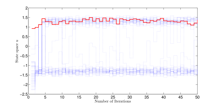
Figure 5: This figure demonstrates the redistribution property of the ETAIS algorithm for a bimodal target with equally weighted modes. Initially there is one chain in the positive mode, and 49 chains in the negative mode.

The biggest issue for the Metropolis-Hastings algorithms when sampling from multimodal posterior distributions is that frequent switches between the modes are required if the method is to converge efficiently. The ETAIS algorithm tackles this problem with its resampling step. The algorithm uses its dynamic mixture proposal distribution to build up an approximation of the posterior at each iteration, and then compares this to the posterior distribution via the weights function. Any large discrepancy in the approximation will result in a large or small weight being assigned to the relevant chain, meaning the chain will either pull other chains towards it or be sucked towards a chain with a larger weight. In this way, the algorithm allows chains to ‘teleport’ to regions of the posterior which are in need of more exploration. Figure 5 shows the trace of a simulation of the ETAIS-RW algorithm for a bimodal example with equally weighted modes, with initially 1 chain in the positive mode, and 49 chains in the negative mode. It takes only a handful of iterations for the algorithm to balance out the chains into 25 chains in each mode. The chains switch modes without having to climb the energy gradient in the middle.

8 Numerical Examples

The numerical examples in this section were all computed on a single core of a Dell server with four 8-core 3.3GHz CPUs and 64Gb memory. Throughout we measure the efficiency of the algorithms in terms of the number of iterations (i.e. likelihood evaluations) which are required in order to reach a given order of accuracy. The reason for this is that this method is designed with a particular type of challenging inverse problem in mind, namely one which is low dimensional, has an expensive likelihood (such as a PDE solve, and/or very large data) which dwarfs the overhead cost of ETAIS, and which could have complex posterior structure, such as correlations, multimodality or other highly non-Gaussian features.

The numerics contained herein compare the ETAIS approach that we have presented against Metropolis-Hastings methods with the same type of proposal as is used by the kernels within ETAIS. Since we propose that ETAIS is a potential framework for parallelised Bayesian computations, we compare ETAIS with $N$ ensemble members against an independent ensemble of $N$ Metropolis-Hastings chains. All implementations were computed in serial, but the results demonstrate a clear speed-up which could be further exploited through parallelisation.

8.1 Automated variance tuning

In this first example, we target a simple 1D Gaussian distribution, in order to show the approximate equivalence of optimising the variance of the proposal kernels using the effective sample size, and the $L^{2}$ error, which of course is not available to us in practical applications.

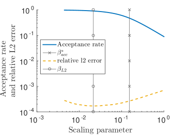
(a) RWMH algorithm.

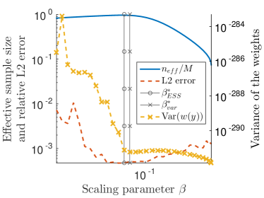
(b) ETAIS-RW algorithm.

Figure 6: Finding optimal values of $\beta$ for a 1D Gaussian density. Bottom left: Convergence of the (A)RWMH and (A)ETAIS-RW algorithms.

Statistic	RWMH
$\beta_{\text{L2}}^{*}$	2.1e-2
$\beta_{\%}^{*}$	1.5e-1
Acceptance Rate ($\beta_{\text{L2}}^{*}$)	9.0e-1
Acceptance Rate ($\beta_{\%}^{*}$)	5.0e-1

Statistic	ETAIS-RW
$\beta_{\text{eff}}^{*}$	4.7e-2
$\beta_{\text{var}(w(y))}^{*}$	5.8e-2
$\beta_{\text{L2}}^{*}$	3.9e-2

Table 1: Optimal values of $\beta$ summarised from Figure 6. Statistics calculated as described in Section 4.1. The values $\beta^{*}_{\text{L2}}$ and $\beta^{*}_{\%}$ are the optimal scaling parameters found by optimising the relative $L^{2}$ errors and acceptance rate respectively. Similarly $\beta_{\text{eff}}^{*}$ and $\beta_{\text{var}(w(y))}^{*}$ optimise the effective sample size and variance of the weights statistics.

Figure 6 (a) shows the two values of $\beta$ which are optimal according to the acceptance rate and relative $L^{2}$ error criteria for the RWMH algorithm. The smaller estimate comes from the relative $L^{2}$ error, and the larger from the acceptance rate. The results in Figure 6 are summarised in Table 1. Since in general we cannot calculate the relative $L^{2}$ error, we must optimise the algorithm using the acceptance rate. From the relative $L^{2}$ error curve we can see that the minimum is very wide and despite the optimal values being very different there is not a large difference in the convergence rate.

Figure 6 (b) shows the effective sample size ratio compared to the error analysis and the variance of the weights. The relative $L^{2}$ error graph is noisy, but it is clear that the maximum in the effective sample size and the minimum in the variance of the weights are both close to the minimum in the relative $L^{2}$ error. Due to this we say that the estimate of the effective sample size found by averaging the statistic over each iteration is a good indicator for the optimal scaling parameter.

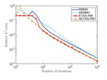
(a) Convergence

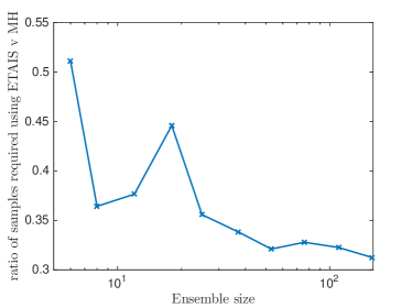
(b) Scaling of ETAIS-RW

Figure 7: Left: Convergence of the (A)RWMH and (A)ETAIS-RW algorithms for a 1D Gaussian. Computed using 50 ensemble members, and the ETPF resampler. Right: Ratio of ETAIS-RW samples required to reach the same tolerance as the RWMH algorithm for a range of ensemble sizes.

Figure 7 (left) shows that the ETAIS-RW algorithm converges to the posterior distribution significantly faster than the RWMH algorithm, in both $L^{2}$ error and relative error in the moments. The adaptive algorithms are also shown in Figure 7. We see that both adaptive algorithms converge to the posterior at a similar speed to the respective optimised algorithm. This shows that, particularly for ETAIS, we can optimise simulations efficiently on the fly.

Figure 7 (right) was produced by identifying the optimal value of the scaling parameter for a range of ensemble sizes, and then computing the ratio of ETAIS samples needed in comparison with RWMH samples for the same level of error. The decreasing trend shows superlinear improvement of ETAIS with respect to ensemble size, in terms of the number of iterations required, which is a demonstration of our belief that communication between the ensemble members should give us added value over and above that provided by naive parallelism. This decrease is due to the increasing effective sample size shown in Figure 2 (b).

8.2 Multimodal targets and the effect of resampler quality

In this second example we investigate the behaviour of the ETAIS algorithm when applied to a bimodal problem, given by a mixture of two Gaussians,

$$\pi(x)=0.2\pi_{1}(x)+0.8\pi_{2}(x),$$

where $\pi_{1}$ is the density of a $\mathcal{N}\left(\begin{pmatrix}1\\ 1\end{pmatrix},\begin{pmatrix}0.1&0\\ 0&0.1\end{pmatrix}\right)$ random variable and $\pi_{2}$ is the density of a $\mathcal{N}\left(\begin{pmatrix}-5\\ -5\end{pmatrix},\begin{pmatrix}2.75&-2.25\\ -2.25&2.75\end{pmatrix}\right)$ random variable.

MH methods can struggle with multimodal problems, particularly where switches between the modes are rare, resulting in incorrectly proportioned modes in the histograms. This example demonstrates that the ETAIS algorithm redistributes samples to new modes as they are found. This means that we expect the number of samples in a mode to be approximately proportional to the probability density in that mode, resulting in faster global convergence. In particular, we will look at the effect of using either the ETPF, MT or a standard bootstrap resampler.

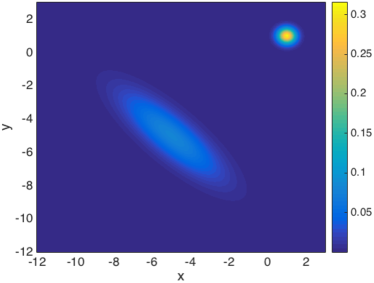
(a) Target density

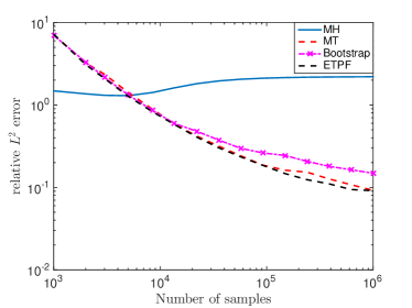
(b) Comparison of resamplers

Figure 8: Left: Bimodal target density. Right: Convergence of RWMH and ETAIS-RW with ETPF, MT and bootstrap resamplers.

Figure 8 shows the bimodal target density, and convergence plots for the RWMH and ETAIS-RW with ETPF, MT and bootstrap resamplers, averaged over 32 repeats. As expected, a higher quality resampler leads to better proposal distributions, which in turn leads to greater stability and more reliable convergence. However, this also shows that the MT is a good greedy approximation of the ETPF, and for a fraction of the cost when the number of ensemble members is larger, as shown in Section 5. The RWMH algorithm fails to converge efficiently since chains only very rarely make switches between the two modes, leading to very slow mixing. This demonstrates the advantage that ensemble-based methods can have over other methods when the target is multimodal.

8.3 A Mixture Model

The technique of mixture modelling employs well known parametric families to construct an approximating distribution which may have a complex structure. Most commonly, Gaussian kernels are used since underlying properties in the data can often be assumed to follow a Gaussian distribution. An example would be if a practitioner were to measure the heights of one hundred adults, but failed to record their gender. The data could be considered as one population with two sub populations, male and female. The problem then might be to find the average height of adult males from the data. In this case, since height is often considered to follow a Gaussian distribution, it makes sense to model the population as a mixture of two univariate Gaussian distributions.

A well known problem in the Bayesian treatment of mixture modelling is that of identification, sometimes referred to as the label-switching phenomenon. The likelihood distribution for mixture models is invariant under permutations of the mixture labels. If a mixture has $n$ means and the point $(\mu_{1},\dots,\mu_{n})$ maximises the likelihood, then the likelihood will also be maximised by $(\mu_{\varphi(1)},\dots,\mu_{\varphi(n)})$ for all permutations $\varphi(\cdot)$. This means that the number of modes in the posterior distribution is of order $\mathcal{O}(n!)$. As we have seen it can be hard for standard MH algorithms to obtain reliable inference for posterior distributions with a large number of modes, or even a small number of modes which are separated by a large distance.

8.3.1 Target Distribution

In particular we look at a data set where we assume that there are two subpopulations within the overall population. Since both subpopulations will be approximated by Gaussian distributions we have five parameters which we need to be estimated, two means $\{\mu_{1},\mu_{2}\}$, two variances $\{\sigma^{2}_{1},\sigma^{2}_{2}\}$, and the probability, $p$, that an individual observation belongs to the first subpopulation. We have 100 data points, $D_{i}$, which we assume to be distributed according to

$$D_{i}\sim p\mathcal{N}(\mu_{1},\sigma^{2}_{1})+(1-p)\mathcal{N}(\mu_{2},\sigma^{2}_{2}),\quad i=1,\dots,100,$$

where $p\in[0,1]$, $\mu_{1},\mu_{2}\in\mathbb{R}$ and $\sigma^{2}_{1},\sigma^{2}_{2}\in\mathbb{R}^{+}$. Due to the domains of these parameters and also some prior knowledge, we assign the priors

$$p\sim\text{Beta}(1,1),\quad\mu_{1,2}\sim\mathcal{N}(0,4)\quad\text{and}\quad\sigma^{2}_{1,2}\sim\text{Gamma}(\alpha=2,\beta=1).$$

If we collect these parameters in the vector $\theta=(p,\mu_{1},\sigma^{2}_{1},\mu_{2},\sigma^{2}_{2})^{\top}$, the resulting posterior distribution is

$$\pi(\theta|D)\propto\prod\limits_{i=1}^{100}(p\mathcal{N}(D_{i};\mu_{1},\sigma^{2}_{1})+(1-p)\mathcal{N}(D_{i};\mu_{2},\sigma^{2}_{2}))\prod\limits_{i=1}^{5}\pi_{0}^{i}(\theta_{i}),$$ (7)

where $\pi_{0}^{i}(\cdot)$ is the prior density function corresponding to $\theta_{i}$.

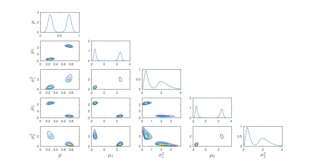
Figure 9: The posterior distribution of $\theta$ as given in Equation (7) as found from 10 million samples from the ETAIS algorithm. The main diagonal contains the marginal distributions of each $\theta_{i}$, and the lower triangular contours represents the correlation between pairs of parameters.

Figure 9 presents a visualisation of the posterior distribution for this problem, created from 10 million samples produced by the ETAIS-RW algorithm.

8.3.2 Implementation

In order to quantify error, we note that the probability density should be evenly divided between the two modes. This is due to the symmetric prior for $p$, and and the same priors being assigned to $\mu_{1}$ and $\mu_{2}$, and also to $\sigma^{2}_{1}$ and $\sigma^{2}_{2}$. To decide which mode a sample belongs to we define a plane which bisects the posterior so that each point on this plane lies exactly halfway between the two true solutions to the inverse problem i.e. the value of $\theta$ used to generate the data, and also the $\theta$ obtained by a relabelling of the parameters. Now that we can assign a sample to a particular mode, we can calculate the density in each mode by summing the weights associated to all samples in that mode,

$$\bar{w}_{k}=\sum\limits_{i=1}^{N}w_{i}I_{X_{i}\in\text{Mode $k$}},\quad k=1,2,$$

and the relative error in the amount of density in each mode is then

$$w_{\text{error}}=2\left|\frac{\bar{w}_{1}}{\bar{w}_{1}+\bar{w}_{2}}-\frac{1}{2}\right|.$$ (8)

Since the probability $p$ is constrained to lie in the interval $[0,1]$, and the variances must be positive, it can be wasteful to use Gaussian proposal distributions, which will produce samples outside of the support of the posterior. Moreover, the value of the variances of the unknown distributions are strictly non-negative. The algorithm will be most efficient if the proposal and posterior distributions are mutually absolutely continuous. It is also useful to be able to pick proposal densities for which the variance is easily scaled so that we can tune them to optimise efficiency. Thus we pick the following proposal distributions for the $p$, $\mu$ and $\sigma^{2}$ parameters, respectively;

$$q_{p}\sim\text{Beta}(\delta^{-2}p,\delta^{-2}(1-p)),\quad q_{\mu_{1,2}}\sim\mathcal{N}(\mu_{1,2},4\delta^{2})\quad\text{and}\quad q_{\sigma^{2}_{1,2}}\sim\text{Gamma}(\alpha^{*},\beta^{*}),$$

where $\alpha^{*}=\sigma^{2}_{1,2}\beta^{*}$, $\beta^{*}=\sigma^{2}_{1,2}/2\delta^{2}$ and $\delta$ is a scaling parameter to be tuned. This means that our proposal distributions will not be a mixture of multivariate Gaussians, but independent mixtures of univariate Beta, Gamma and Gaussian distributions.

In the numerics which follow we have increased the ensemble size from $M=50$ to $M=500$ to compensate for the increase in dimension. We also use the MT algorithm for the resampling step because of the reduced computational cost. The method otherwise remains the same as in previous examples. We perform test runs to find the optimal scaling parameters considering convergence to modes with equal density. We then calculate the convergence rates of the algorithms by producing 10 million samples from the posterior with each algorithm, and repeat the simulation 32 times.

8.3.3 Convergence of MH vs ETAIS

Algorithm	MH	ETAIS
$\delta^{*}$	1.3e-1	2.3e-1

Table 2: Optimal values of the scaling parameter. The MH algorithm is optimised using the acceptance rate, and the ETAIS algorithm is optimised using the effective sample size.

The optimal scaling parameters for the MH and ETAIS algorithms with the proposal distributions described in Section 8.3.2 are given in Table 2.

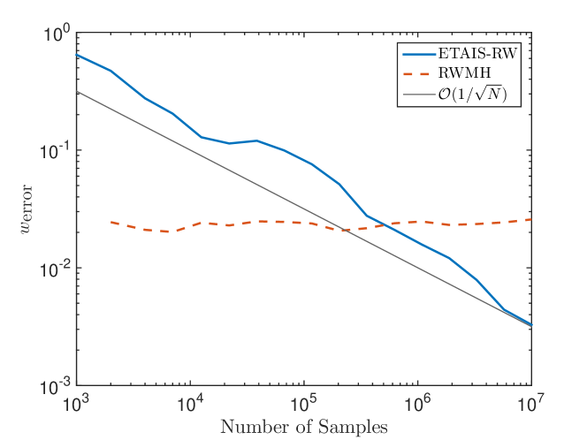
Figure 10: Convergence of the ETAIS algorithm for the mixture model described in Section 8.3, convergence judged using the criterion in Equation (8). Implementation described in Sections 8.3.2 and 8.3.3. Resampling is performed using the MT scheme.

Convergence of the relative error for the two algorithms is displayed in Figure 10. ETAIS converges at the expected $\mathcal{O}(1/\sqrt{N})$ rate, whereas the MH algorithm converges to locally smooth histograms but with the wrong proportion of samples in each mode. The relatively low value of the error for the MH example is due to the priors covering the sample space evenly, however since transitions are near impossible with a small value of the scaling parameter, this error will take a very long time to reduce. This problem was discussed in Section 8.2.

In this example, we have only considered a relatively low dimensional mixture model problem, with only two distributions in the mixture. With more elements in the mixture, and/or an undefined number in the mixture, the dimension of this problem will quickly increase. Importance sampling schemes such as this suffer from the curse of dimensionality, limiting the size of the dimension of target density that it can efficiently sample from. However, this example does demonstrate the remarkable convergence of the ETAIS for multimodal target distributions.

8.4 Data assimilation with Lorenz ‘63 trajectories

The sampling algorithm we have introduced in this paper is designed for problems where the likelihood density function is expensive to calculate, and the computational overhead involved in the calculation of the importance weights is dwarfed. This situation commonly occurs in inverse problems where the model being investigated involves the solution of a differential equation. In this example we attempt to recover the initial position of a particle with motion governed by Lorenz’s 1963 atmospheric convection equations [28]:

$$\frac{\text{d}x}{\text{d}t} =\sigma(y-x),$$

$$\frac{\text{d}y}{\text{d}t} =x(\rho-z)-y,$$

$$\frac{\text{d}z}{\text{d}t} =xy-\beta z.$$

When the parameters are chosen to be $\rho=28$, $\sigma=10$ and $\beta=8/3$ this system has chaotic solutions. If we are interesting in calculating the initial position by observing the location of the particle at certain points in time, it can quickly become intractable when there is any noise in the observations.

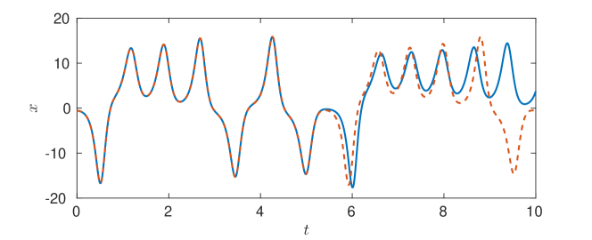
Figure 11: Trajectory of the $x$ component of a particles position varying in time when motion is governed by the Lorenz ‘63 equations. The two trajectories are calculated using an initial position of $[-0.587,-0.563,16.870]$ and $[-0.590,-0.563,16.870]$.

To demonstrate how small errors in the initial condition of a Lorenz solution can affect the trajectory of a particle, Figure 11 shows the path taken by two particles with very similar initial conditions,

$$\mathbf{x}_{0}^{1}=\begin{pmatrix}-0.587\\ -0.563\\ 16.870\end{pmatrix}\quad\text{and}\quad\mathbf{x}_{0}^{2}=\begin{pmatrix}-0.590\\ -0.563\\ 16.870\end{pmatrix}.$$

This small difference in the $x$-dimension of the initial condition leads to the trajectories of the two particles decoupling near $t=5$. This chaotic behaviour means that if we take only a few observations over a long time period we will find that many trajectories which may be vastly different achieve similar values of the likelihood function and so the posterior distribution for the initial condition can become very complex.

8.4.1 Target Distribution

For this example, we observe noisily the position of a particle at ten equally spaced points in the time interval $t\in(0,1]$. The Lorenz equations are solved with the chaotic parameters given above and the initial condition $\mathbf{x}_{0}^{1}$. A time step of $h=1\times 10^{-3}$ was used to evolve the equations numerically with the explicit Euler method. The noise added to each observation was taken from the distribution $\mathcal{N}(0,0.1^{2}I)$. Priors for the initial condition coordinates were given by

$$x_{0}\sim\mathcal{N}(-0.5,0.4^{2}),\quad y_{0}\sim\mathcal{N}(-0.5,0.4^{2})\quad\text{and}\quad z_{0}\sim\mathcal{N}(15,0.4^{2}).$$

The posterior density function takes the form

$$\pi(\mathbf{x}_{0}|D)\propto\exp\left\{-\frac{1}{2}\|\mathcal{G}(\mathbf{x}_{0})-D\|^{2}_{\Sigma}\right\}\mathcal{N}(\mathbf{x}_{0};m,0.4^{2}\text{I}),$$

where $\mathcal{G}$ calculates the solution to the Lorenz equations, using the Euler method with a time step of $h=1\times 10^{-3}$ starting at the initial condition $\mathbf{x}_{0}$, and returns the position at $t=0.1,...,1$. The mean of the prior distribution $m=[-0.5,-0.5,15]$.

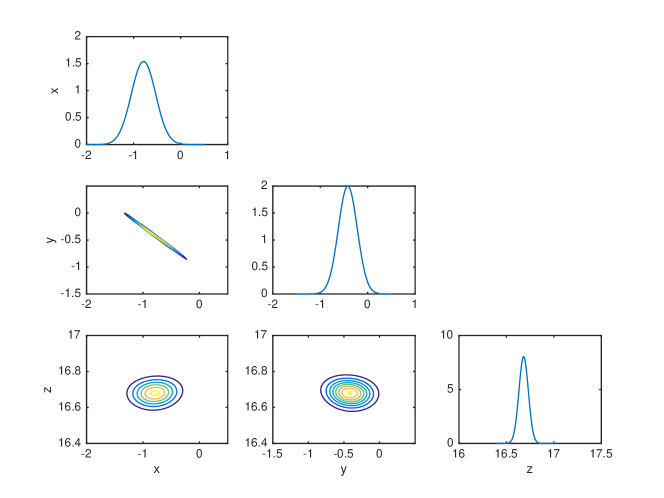
Figure 12: Posterior distribution for the initial condition of the particle with motion governed by the Lorenz equations as described in Section 8.4.1.

Figure 12 shows the marginal distributions of the posterior distribution for the initial condition $\mathbf{x}_{0}$ as found using the MH algorithm. While the $z$-dimension is largely uncorrelated with the other two dimensions, the correlation between $x$ and $y$ is -0.97, which makes it a challenging posterior distribution to explore without a transformation of the parameter space.

8.4.2 Implementation

As in the previous example, we have no analytic form for the normalisation constant of the posterior and so we will measure convergence of the algorithms by calculating convergence to the posterior mean, where the truth is calculated using a very long chain produced by the MH algorithm.

For this example, we use an ensemble size of $M=1500$, and the MT resampling algorithm. The optimal scaling parameters are calculated for both algorithms using test runs which are not included in the convergence cost calculations. Convergence graphs are produced using 32 repeats of each algorithm with each simulation producing one million samples.

8.4.3 Convergence of MH vs ETAIS

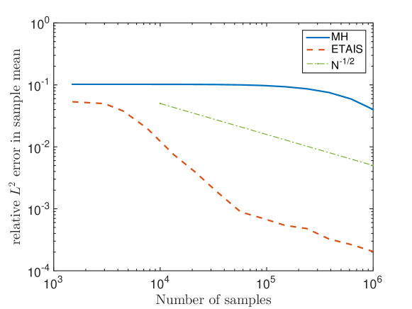
Figure 13: Convergence of the sample mean to the posterior mean for the MH and ETAIS algorithms. Posterior distribution as described in Section 8.4.1.

Figure 13 shows convergence plots for this problem using RWMH and ETAIS. The burn-in of the ETAIS is remarkably better than MH, as the ensemble quickly covers the manifold on which the majority of the density lies close to. The plot shows convergence with respect to number of samples, but the two approaches have differing costs, due to the calculation of the denominator in the weights in the ETAIS, and the resampling step (MT). Assuming that both error curves decay like $N^{-1/2}$ from $N=10^{6}$, then for a given error tolerance, the number $N_{\rm MH}$ of MH samples required is given by

$$N_{\rm MH}=N_{\rm ETAIS}\times 3.838\times 10^{4},$$

where $N_{\rm ETAIS}$ is the number of ETAIS samples required for the same error tolerance. The cost per sample for the MH and ETAIS methods for this problem are $1.64\times 10^{-5}$ and $1.46\times 10^{-3}$ respectively. Here the ETAIS results were produced with a serial implementation, so this cost may be slightly overoptimistic, since the runtimes do not include extra overheads of communicating the ensemble states between processors. However, putting this together, we arrive at a speed-up factor of over 430, which will undoubtedly overshadow any such underestimate of the cost-per-sample of the ETAIS approach. This demonstrates the benefits of this approach for problems with expensive likelihoods and challenging posteriors such as this one.

9 Discussion and Conclusions

We have explored the application of low dimensional Bayesian inverse problems. We have demonstrated numerically that this method converges faster than the analogous naively parallelised Metropolis-Hastings algorithms. Further experimentation with the Metropolis Adjusted Langevin Algorithm (MALA), preconditioned Crank-Nicolson (pCN), preconditioned Crank-Nicolson Langevin (pCNL) and Hamiltonian Monte Carlo (HMC) proposals has yielded similar results[42].

The implementations of the ETAIS that have been presented in this paper, have been run in serial, but we argue that, particularly for inverse problems with expensive likelihoods, for example in the case where this requires the approximation of the solution of a differential equation, that this method is an excellent candidate for parallelisation, with the likelihood evaluations for each particle being computed on a different processor. This said, the numerical results that we have presented demonstrate that even a serial implementation can outperform standard Metropolis-Hastings methods.

The ETAIS has a number of favourable features, for example the algorithm’s ability to redistribute, through the resampling regime, the ensemble members to regions which require more exploration. This allows the method to be used to sample from complex multimodal distributions.

Another strength of the ETAIS is that it can also be used with any MCMC proposal. There are a growing number of increasing sophisticated MCMC algorithms (non-reversible Langevin/HMC proposals, Riemann manifold MCMC etc) which could be incorporated into this framework, leading to even more efficient algorithms, and this is another opportunity for future work.

One limitation of the ETAIS approach as described above is that a direct solver of the ETPF problem (such as FastEMD [35]) has computational cost $\mathcal{O}(M^{3}\log M)$, where $M$ is the number of particles in the ensemble. As such, we introduced a more approximate resampler the approximate multinomial resampler, which allows us to push the approach to the limit with much larger ensemble sizes. The ETAIS framework is very flexible in terms of being able to use any combination of proposal distributions and resampling algorithms that one wishes.

We have demonstrated that the framework that we have considered, with the use of state-of-the-art optimal transport-based resampling, can reduce the number of likelihood evaluations required to characterise complex posterior distributions in low dimensions to a given degree. We have also introduced a greedy approximation to this resampler, which drastically reduces the cost, at the loss of some accuracy, which can be mitigated with the use of larger ensembles. We have detailed how scaling parameters in the MCMC proposals that are used within the mixture distribution can be quickly and efficiently tuned in an automated way. Lastly we have demonstrated that when the likelihood is expensive, for instance because it involves the numerical approximation of the solution of a differential equation, that we can achieve orders of magnitude reductions in cost to reach a given error tolerance in comparison with standard Metropolis-Hastings approaches.

However, tuning the variances and covariances of the mixture proposal components globally is likely to be of limited use for multimodal problems where the modes have very different covariances, or where there are curved ridges in the density. With increased dimensionality and/or complexity of the target the distribution, we also require increases in the size of the ensemble if we wish to have a stable ETAIS implementation. After a certain point, the extra overheads associated with a very large ensemble will outweigh the advantages of this approach. However, there are a variety of possible solutions to this problem that would be worthy of future consideration, not least the potential to use transport maps[17, 34] to map Gaussian mixtures to highly complex non-Gaussian approximations of the posterior. Such a map could encode local covariance information, and lead to accelerated and stable ETAIS sampling with much smaller ensemble sizes.

Appendix A Glossary of acronyms

Acronym	Full name
MCMC	Markov chain Monte Carlo
RWMH	Random walk Metropolis-Hastings
MALA	Metropolis-adjusted Langevin algorithm
AIS	Adaptive importance sampling
PMC	Population Monte Carlo
ETAIS	Ensemble transport adaptive importance sampling
ETPF	Ensemble transport particle filter
MT	Multinomial transformation
ETAIS-X	ETAIS with X kernels
AETAIS-X	Adaptive ETAIS with X kernels

References

- [1] C. Andrieu, É. Moulines, et al., On the ergodicity properties of some adaptive MCMC algorithms, The Annals of Applied Probability, 16 (2006), pp. 1462–1505.
- [2] E. Angelino, E. Kohler, A. Waterland, M. Seltzer, and R. Adams, Accelerating MCMC via parallel predictive prefetching, arXiv preprint arXiv:1403.7265, (2014).
- [3] J. Bierkens, Non-reversible Metropolis-Hastings, Statistics and Computing, (2015), pp. 1–16.
- [4] M. Bink, M. Boer, C. Ter Braak, J. Jansen, R. Voorrips, and W. Van de Weg, Bayesian analysis of complex traits in pedigreed plant populations, Euphytica, 161 (2008), pp. 85–96.
- [5] M. Bugallo, L. Martino, and J. Corander, Adaptive importance sampling in signal processing, Digital Signal Processing, 47 (2015), pp. 36–49.
- [6] T. Bui-Thanh and M. Girolami, Solving large-scale PDE-constrained Bayesian inverse problems with Riemann manifold Hamiltonian Monte Carlo, Inverse Problems, 30 (2014), p. 114014.
- [7] B. Calderhead, A general construction for parallelizing Metropolis- Hastings algorithms, Proceedings of the National Academy of Sciences, 111 (2014), pp. 17408–17413.
- [8] O. Cappé, R. Douc, A. Guillin, J.-M. Marin, and C. Robert, Adaptive importance sampling in general mixture classes, Statistics and Computing, 18 (2008), pp. 447–459.
- [9] O. Cappé, A. Guillin, J. Marin, and C. Robert, Population Monte Carlo for ion channel restoration.
- [10] O. Cappé, A. Guillin, J. Marin, and C. Robert, Population monte carlo, Journal of Computational and Graphical Statistics, (2012).
- [11] G. Celeux, J. Marin, and C. Robert, Iterated importance sampling in missing data problems, Computational statistics & data analysis, 50 (2006), pp. 3386–3404.
- [12] J. Cornuet, J. Marin, A. Mira, and C. Robert, Adaptive multiple importance sampling, Scandinavian Journal of Statistics, 39 (2012), pp. 798–812.
- [13] C. Cotter and S. Reich, Ensemble filter techniques for intermittent data assimilation-a survey, in Large Scale Inverse Problems. Computational Methods and Applications in the Earth Sciences, Walter de Gruyter, Berlin, 2012, pp. 91–134.
- [14] S. Cotter, G. Roberts, A. Stuart, and D. White, MCMC methods for functions: modifying old algorithms to make them faster, Statistical Science, 28 (2013), pp. 424–446.
- [15] R. Douc, A. Guillin, J. Marin, C. Robert, et al., Convergence of adaptive mixtures of importance sampling schemes, The Annals of Statistics, 35 (2007), pp. 420–448.
- [16] R. Douc, A. Guillin, J.-M. Marin, and C. Robert, Minimum variance importance sampling via population monte carlo, ESAIM: Probability and Statistics, 11 (2007), pp. 427–447.
- [17] T. El Moselhy and Y. Marzouk, Bayesian inference with optimal maps, Journal of Computational Physics, 231 (2012), pp. 7815–7850.
- [18] V. Elvira, L. Martino, D. Luengo, and journal=Signal Processing volume=131 pages=77–91 year=2017 publisher=Elsevier Bugallo, M., Improving population monte carlo: Alternative weighting and resampling schemes.
- [19] G. Evensen, Sequential data assimilation with a nonlinear quasi-geostrophic model using Monte Carlo methods to forecast error statistics, Journal of Geophysical Research: Oceans (1978–2012), 99 (1994), pp. 10143–10162.
- [20] M. Girolami and B. Calderhead, Riemann manifold Langevin and Hamiltonian Monte Carlo methods, Journal of the Royal Statistical Society: Series B (Statistical Methodology), 73 (2011), pp. 123–214.
- [21] H. Haario, E. Saksman, and J. Tamminen, Componentwise adaptation for high dimensional MCMC, Computational Statistics, 20 (2005), pp. 265–273.
- [22] W. Hastings, Monte Carlo sampling methods using Markov chains and their applications, Biometrika, 57 (1970), pp. 97–109.
- [23] T. House, A. Ford, S. Lan, S. Bilson, E. Buckingham-Jeffery, and M. Girolami, Bayesian uncertainty quantification for transmissibility of influenza, norovirus and ebola using information geometry, Journal of The Royal Society Interface, 13 (2016), p. 20160279.
- [24] M. Isard and A. Blake, Condensation—conditional density propagation for visual tracking, International journal of computer vision, 29 (1998), pp. 5–28.
- [25] C. Ji and S. C. Schmidler, Adaptive Markov Chain Monte Carlo for Bayesian Variable Selection, Journal of Computational and Graphical Statistics, 22 (2013), pp. 708–728.
- [26] J. Liu, Monte Carlo strategies in scientific computing, Springer Science & Business Media, 2008.
- [27] J. Liu, F. Liang, and W. Wong, The multiple-try method and local optimization in Metropolis sampling, Journal of the American Statistical Association, 95 (2000), pp. 121–134.
- [28] E. Lorenz, Deterministic nonperiodic flow, Journal of the atmospheric sciences, 20 (1963), pp. 130–141.
- [29] J.-M. Marin, K. Mengersen, and C. Robert, Bayesian modelling and inference on mixtures of distributions, Handbook of statistics, 25 (2005), pp. 459–507.
- [30] L. Martino, V. Elvira, D. Luengo, and J. Corander, An adaptive population importance sampler: Learning from uncertainty, IEEE Transactions on Signal Processing, 63 (2015), pp. 4422–4437.
- [31] , Layered adaptive importance sampling, Statistics and Computing, 27 (2017), pp. 599–623.
- [32] G. Moore et al., Cramming more components onto integrated circuits, Proceedings of the IEEE, 86 (1998), pp. 82–85.
- [33] R. Neal, MCMC using ensembles of states for problems with fast and slow variables such as Gaussian process regression, arXiv preprint arXiv:1101.0387, (2011).
- [34] M. Parno and Y. Marzouk, Transport map accelerated markov chain monte carlo, arXiv preprint arXiv:1412.5492, (2014).
- [35] O. Pele and M. Werman, Fast and robust Earth mover’s distances, in Computer Vision, 2009 IEEE 12th International Conference on, IEEE, 2009, pp. 460–467.
- [36] S. Reich, A nonparametric ensemble transform method for Bayesian inference, SIAM Journal on Scientific Computing, 35 (2013), pp. A2013–A2024.
- [37] C. Robert and G. Casella, Monte Carlo statistical methods, Springer Science & Business Media, 2013.
- [38] G. Roberts and J. Rosenthal, Optimal scaling of discrete approximations to Langevin diffusions, Journal of the Royal Statistical Society: Series B (Statistical Methodology), 60 (1998), pp. 255–268.
- [39] , Optimal scaling for various Metropolis-Hastings algorithms, Statistical science, 16 (2001), pp. 351–367.
- [40] , Coupling and ergodicity of adaptive Markov chain Monte Carlo algorithms, Journal of Applied Probability, 44 (2007), pp. 458–475.
- [41] , Examples of adaptive MCMC, Journal of Computational and Graphical Statistics, 18 (2009), pp. 349–367.
- [42] P. Russell, PhD Thesis, PhD thesis, School of Mathematics, University of Manchester, 2017.
- [43] J. Sexton and D. Weingarten, Hamiltonian evolution for the hybrid Monte Carlo algorithm, Nuclear Physics B, 380 (1992), pp. 665–677.
- [44] J. Sirén, P. Marttinen, and J. Corander, Reconstructing population histories from single nucleotide polymorphism data, Molecular biology and evolution, 28 (2011), pp. 673–683.
- [45] A. Solonen, P. Ollinaho, M. Laine, H. Haario, J. Tamminen, H. Järvinen, et al., Efficient MCMC for climate model parameter estimation: parallel adaptive chains and early rejection, Bayesian Analysis, 7 (2012), pp. 715–736.