Power Allocation in Multi-hop OFDM Transmission Systems with Amplify-and-Forward Relaying: A Unified Approach

Abstract

In this paper a unified approach for power allocation (PA) problem in multi-hop orthogonal frequency division multiplexing (OFDM) amplify-and-forward (AF) relaying systems has been developed. In the proposed approach, we consider short and long-term individual and total power constraints at the source and relays, and devise decentralized low complexity PA algorithms when wireless links are subject to channel path-loss and small-scale Rayleigh fading. In particular, aiming at improving the instantaneous rate of multi-hop transmission systems with AF relaying, we develop (i) a near-optimal iterative PA algorithm based on the exact analysis of the received SNR at the destination; (ii) a low complexity-suboptimal iterative PA algorithm based on an approximate expression at high-SNR regime; and (iii) a low complexity-non iterative PA scheme with limited performance loss. Since the PA problem in multi-hop systems is too complex to solve with known optimization solvers, in the proposed formulations, we adopted a two-stage approach, including a power distribution phase among distinct subcarriers, and a power allocation phase among different relays. The individual PA phases are then appropriately linked through an iterative method which tries to compensate the performance loss caused by the distinct two-stage approach. Simulation results show the superior performance of the proposed power allocation algorithms.

I Introduction

Multi-hop relaying and orthogonal frequency division multiplexing (OFDM) are promising techniques for high-speed data communication among wireless devices that may not be within direct transmission range of each other. Relaying protocols are broadly categorized as amplify-and-forward (AF) relaying, in which each relay forwards a scaled version of the received noisy copy of the source signal, and decode-and-forward (DF) relaying, in which each relay forwards a regenerated version of the received noisy copy of the source signal. AF relays may also be categorized as blind/fixed gain, channel assisted, and channel noise assisted, based on how source-relay channel state information (CSI) and noise statistics affect the relay gains [1]. The capacity analysis and transmission protocol design over relay channels have attracted lots of research activities in the past decade [2]- [4]. As relays have shown their merit for data transfer purposes, multi-hop communications have been also included in advanced wireless standards such as IEEE 802.11n [5], WiMAX, and LTE-Advanced [6]- [9]. To achieve power efficiency in multi-hop transmission systems, it is necessary to devise efficient power allocation (PA) strategies for the source and intermediate relays, when a multi-hop data transmission path is setup. For the simplest form of dual-hop relaying systems, the PA problem has been investigated in [10]- [15]. Specifically in [15], for a two-hop OFDM communication system with a given power budget, the authors presented the optimal power allocation at the relay (source) node for a given source (relay) power allocation scheme, that maximizes the instantaneous rate of the system. Then, using simulations they showed that by iterative power allocation between source and relay, a higher gain is achieved. A jointly optimal subcarrier pairing and power allocation scheme which maximizes the throughput of OFDM amplify-and-forward relaying systems subject to a statistical delay constraint is investigated in [16]. Power allocation for dual-hop OFDM relaying systems has been also considered in [17]- [23]. The power allocation problem for relaying system models with more than two hops over narrowband fading channels has been considered in [24], [25]. Especially in [25], aiming at maximizing the instantaneous rate, the power allocation solution for AF relaying protocol over narrowband Rayleigh fading channels has been provided. In [26] a path searching algorithm has been presented to find the best links among relays and then two subcarrier allocation algorithms are presented which aim at resource utilization improvement. Optimal and suboptimal power allocation schemes for multi-hop OFDM systems with DF relaying protocol has been developed in [27]. Adaptive power allocation algorithms for maximizing system capacity (when full CSI is available), and minimizing system outage probability (with limited CSI) have been proposed in [28] for multi-hop DF transmission systems under a total power constraint. Aiming at maximizing the end-to-end average transmission rate under a long-term total power constraint, the authors in [29] developed a resource allocation scheme for multi-hop OFDM DF relaying system in which the power allocated to each subcarrier and the transmission time per hop have been specified. In [30], the authors proposed the solution for power allocation problem in multi-hop OFDM relaying system (AF and DF) under total short-term power constraint, where the PA and capacity analysis is developed based on a high SNR approximation in the AF relaying protocol. The approximation used in [30] has been originally proposed in [31] and performs well for small number of hops with high received SNR. In low-to-medium SNR regime or for multi-hop systems with more than three hops, this approximation loses its functionality in design of PA schemes. The multi-hop OFDM transmission system has been also considered in [32], where joint power allocation and subcarrier pairing solutions for AF and DF relaying protocols have been devised under short-term total power constraint. The analysis for AF relaying protocol in [32] is also based on the high SNR approximation as discussed above.

I-A Paper’s contributions

Although several research works have been reported on the power allocation problem in multi-hop OFDM systems, to the best of the author’s knowledge, no attempt has been made to develop a unifying approach addressing different aspect of these systems. In this paper, we focus on multi-hop OFDM systems with AF relaying and different system power constraints. We developed an unified framework for efficient power allocation which includes both iterative and non-iterative solutions. In particular, aiming at maximizing the instantaneous system rate under individual and total short and long-term power constraints, the following power allocation schemes have been devised: (i) A near-optimal iterative PA algorithm which is developed based on the analysis of an exact expression for the received SNR at the destination; (ii) A low complexity-suboptimal iterative PA algorithm in which we use an high-SNR approximation of the system rate for design purposes; and (iii) A low complexity-non iterative PA scheme based on a high-SNR rate analysis at the destination. The rest of this paper is organized as follows. In Section II we introduce the system model and the power allocation problem formulation. An iterative PA solution based on the analysis of the exact destination SNR is presented in Section III. In Section IV we provided sub-optimal PA schemes based on the analysis of an approximated high SNR expression at the destination. Simulation results are provided in Section IV, and concluding remarks are presented in Section V.

II System Model and Problem Formulation

Fig. 1 shows the multi-hop transmission system model under consideration, where OFDM is utilized for broadband communication among the consecutive nodes. We assume that the system uses a routing algorithm, and therefore the path between the source and destination nodes is already established. Here the source node, $T_{0}$, sends data bits to the destination node $T_{N}$ via $N$-1 intermediate relay nodes, $T_{1},T_{2},\ldots,T_{N-1}$, over orthogonal time slots and orthogonal subcarriers. The fading gain of the narrowband subchannel $i$ (corresponding to the $i$th subcarrier) between nodes $T_{k-1}$ and $T_{k}$, denoted by $a_{k,i}$, is modeled as a zero mean circularly symmetric complex Gaussian random variable with variance $\sigma_{k,i}^{2}$. In an AF multi-hop relaying system, each relay first amplifies the signal received from its immediate preceding node, and then forwards it to the next node in the subsequent time slot. The amplification gain in $i$th subcarrier of node $T_{k}$ is adapted based on the instantaneous fading amplitude of the channel between nodes $T_{k-1}$ and $T_{k}$, i.e. $\lvert a_{k,i}\rvert$. To ensure an output relay transmit power $P_{k,i}$ on $i$th subcarrier, the amplification gain is adjusted as [15]:

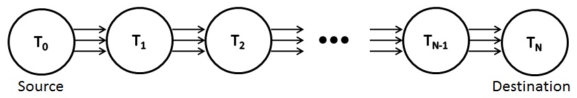
Figure 1: Multi-hop OFDM relaying system with $N$-1 intermediate relays.

$$\begin{array}[]{l}A_{{k,i}}^{2}=\frac{{P}_{{k,i}}}{{P}_{{k-1,i}}{\lvert a_{{k,i}}\rvert^{2}}+N_{{0}_{k,i}}}\;\hskip 17.07164pt\text{for}\hskip 11.38109ptk=1,\ldots,N-1;i=1,\ldots,N_{F}\end{array}$$

where $P_{{0},i}$ and $P_{k,i}$ denote the transmission powers at source and $k$th relay for $i$th subcarrier, respectively. In this model, the number of subcarriers, i.e., the number of points for fast Fourier transform (FFT), and the noise power at $k$th relay within $i$th subcarrier are denoted by $N_{F}$ and $N_{{0}_{k,i}}$ respectively.

For the considered multi-hop OFDM system model, the instantaneous received SNR over the $i$th subcarrier at the destination node is given by

$$\begin{array}[]{l}\gamma_{T}^{i}=\left(\prod_{k=1}^{N}(1+\frac{1}{\tilde{\gamma}_{k,i}})-1\right)^{-1},\end{array}$$ (1)

where $\tilde{\gamma}_{k,i}={\frac{P_{k-1,i}}{{N_{{0}}}_{k,i}}}\lvert{a_{k,i}}\rvert^{2}$ denotes the instantaneous received SNR over the $i$th subcarrier of $k$th hop with the average $\tilde{\Gamma}_{k,i}={\frac{P_{k-1,i}}{{N_{{0}}}_{k,i}}}{{\sigma_{k,i}^{2}}}$. Using (1), the instantaneous rate of the end-to-end multi-hop system is given by

$$\begin{array}[]{l}C=\frac{1}{N}\sum_{i=1}^{N_{F}}{\log(1+\gamma_{T}^{i})}.\end{array}$$ (2)

Considering $\alpha_{k,i}=\frac{P_{k,i}}{P_{T}}$ and ${\gamma}_{k,i}=\frac{P_{T}{\lvert a_{k,i}\rvert}^{2}}{{N_{{0}}}_{k,i}}$, $C$ may be rewritten as follows

$$\begin{array}[]{l}C=\frac{1}{N}\sum_{i=1}^{N_{F}}{\log\left(1+\frac{1}{\prod_{k=1}^{N}(1+\frac{1}{{\alpha_{k,i}\gamma}_{k,i}})-1}\right)}.\end{array}$$ (3)

In a Rayleigh fading environment, ${\gamma}_{k,i}$ follows an exponential distribution with the average ${\Gamma}_{k,i}=\frac{P_{T}{\sigma_{k,i}}^{2}}{{N_{{0}}}_{k,i}}$.

Given the power constraint, here the goal is to find the transmit powers of the subcarriers at the source and the relay nodes such that the instantaneous rate in (3) is maximized. In this paper, we consider power allocation optimization problem under short-term power constraints (STPC), long-term individual power constraints (LTIPC), and long-term total power constraints (LTTPC). The general form of power allocation optimization (PA) problem in this work is as follows.

$$\begin{array}[]{l}\hskip 14.22636pt\max_{\alpha_{k,i}}\quad C\qquad\mathrm{s.t.}\\ \quad\sum_{i=1}^{N_{F}}\sum_{k=0}^{N-1}\alpha_{k,i}=1\hskip 51.21495pt\text{STPC}\\ \\ \quad\mathbb{E}(\alpha_{k,i})=\frac{1}{N\times N_{F}}\hskip 68.2866pt\text{LTIPC}\\ \\ \quad\sum_{i=1}^{N_{F}}\sum_{k=0}^{N-1}\mathbb{E}(\alpha_{k,i})=1\hskip 36.98857pt\text{LTTPC}\\ \end{array}$$ (4)

To explicitly identify the way power is distributed among different subcarriers and nodes, we denote by $P_{i}$ and $P_{k,i}$, respectively, the allocated power to $i$th subcarrier (for all nodes) and the allocated power to $i$th subcarrier in $k$th node (hop). We also define two new nonnegative PA coefficients $\mu_{i}$ and $\beta_{k,i}$ as follows

$$P_{i}= \mu_{i}\times P_{T}$$ (5)

$$\text{and}\quad P_{k,i}= \beta_{k,i}\times P_{i}=\beta_{k,i}\times\mu_{i}\times P_{T},$$ (6)

where $\alpha_{k,i}=\beta_{k,i}\times\mu_{i}$. The optimization problem (3) may now be rewritten as follows with $\mu_{i}$ and $\beta_{k,i}$ as optimization variables,

$$\begin{array}[]{l}\hskip 14.22636pt\max_{\beta_{k,i},\mu_{i}}\quad C\qquad\mathrm{s.t.}\\ \mathrm{C1.}\\ \hskip 17.07164pt\sum_{i=1}^{N_{F}}\sum_{k=0}^{N-1}\mu_{i}\beta_{k,i}=1\hskip 71.13188pt\text{STPC}\\ \hskip 17.07164pt\mathbb{E}(\mu_{i})=\frac{1}{N_{F}},\quad\mathbb{E}(\beta_{k,i})=\frac{1}{N}\hskip 48.36967pt\text{LTIPC}\\ \hskip 17.07164pt\sum_{i=1}^{N_{F}}\mathbb{E}(\mu_{i})=1\quad\sum_{k=0}^{N-1}\mathbb{E}(\beta_{k,i})=1\hskip 5.69054pt\text{LTTPC}\\ \mathrm{C2.}\quad\mu_{i}\geq 0\quad i=1,\ldots,N_{F}\\ \mathrm{C3.}\quad\beta_{k,i}\geq 0\quad k=0,\ldots,N-1;i=1,\ldots,N_{F}.\end{array}$$ (7)

We note that the allocation of power to subcarriers (by finding $\mu_{i}$) and to subcarrier per node (by finding $\beta_{k,i}$) in problem (6) is equivalent to finding $\alpha_{k,i}$ in (3). Unfortunately, the power allocation problems (3) and (6) are too complicated and cannot be solved with known optimization solvers. Hence, in the subsequent sections to find efficient solutions to (7) under different power constraints, we develop iterative and non-iterative algorithms based on the exact and approximate SNR expressions.

III Iterative Power Allocation

In this Section, we consider the power allocation problem (6) as alternate maximization over two simpler power allocation optimization sub-problems. In the first sub-problem, the optimized $\{\beta_{k,i}\}$ is obtained assuming that $\{\mu_{i}\}$ is available. In the second sub-problem, $\{\mu_{i}\}$ is determined for a given set of $\{\beta_{k,i}\}$. Next, we provide an iterative PA algorithm in which the two subproblems are alternately considered with the output of one as the input of the other. Numerical evaluation in Section V verifies the effectiveness of the proposed approach.

III-A Sub-problem 1: Power allocation among relays

Given that the power allocated to each of the subcarriers $\{\mu_{i}\}$ is already known, the power allocation problem among relays in one subcarrier is equivalent to the power allocation problem in a multi-hop system with narrowband fading model. Here, we provide optimal solutions for the PA problems in multi-hop narrowband communication systems with individual long-term and total power constraints. We note that in an AF multi-hop transmission system, maximization of the instantaneous rate of the system is equivalent to maximizing the instantaneous received SNR [25]. The instantaneous received SNR at the destination of multi-hop system given in (1) may be expressed as follows:

$$\begin{array}[]{l}\ln\left(1+{\gamma_{T}^{i}}^{-1}\right)=\ln\prod_{k=1}^{N}(1+\frac{1}{\tilde{\gamma}_{k,i}})=\sum_{k=1}^{N}\ln(1+\frac{1}{{\tilde{\gamma}_{k,i}}}).\end{array}$$

Then, $\gamma_{T}^{i}$ is found as

$$\begin{array}[]{l}\gamma_{T}^{i}=\left[\exp\left(\sum_{k=1}^{N}\ln(1+\frac{1}{\tilde{\gamma}_{k,i}})\right)-1\right]^{-1}.\end{array}$$ (8)

Since, maximizing $\gamma_{T}^{i}$ is equivalent to minimizing the argument of exponential function on the right hand side of (8), we can conclude that

$$\begin{array}[]{l}\text{arg}\max_{\{\beta_{k,i}\}}\gamma_{T}^{i}=\text{arg}\min_{\{\beta_{k,i}\}}{\sum_{k=1}^{N}\ln(1+\frac{1}{\tilde{\gamma}_{k,i}})}.\end{array}$$ (9)

Using (9), the optimization problem for the $i$th subcarrier under LTIPC is written as follows:

$$\begin{array}[]{l}\hskip 14.22636pt\min_{\{\beta_{k,i}\}}\quad\sum_{k=0}^{N-1}\ln(1+\frac{1}{\beta_{k,i}\mu_{i}\gamma_{k+1,i}})\\ \\ \mathrm{s.t.}\quad\mathbb{E}(\beta_{k,i})=\frac{1}{N},\quad k=0,1,\ldots,N-1,\end{array}$$ (10)

where $\{\mu_{i}\}$ is given. In appendix A, it is shown that the objective function in (10) is convex. Since the constraints are linear the main problem is convex, and therefore we use the Lagrange method to obtain the optimal solution. The Lagrangian function is given by

$$\begin{array}[]{l}\mathcal{L}=\sum_{k=0}^{N-1}\ln(1+\frac{1}{\beta_{k,i}\mu_{i}\gamma_{k+1,i}})+\sum_{k=0}^{N-1}\lambda_{k}\left(\mathbb{E}(\beta_{k})-\frac{1}{N}\right)\\ \end{array}$$ (11)

where $\{\lambda_{k,i}\}_{k=0}^{N-1}$ are Lagrange multipliers. By taking the derivative of $\mathcal{L}$ with respect to $\beta_{k,i},k=0,1,...,N-1$, one obtains

$$\begin{array}[]{l}\frac{\partial\mathcal{L}}{\partial\beta_{k,i}}=0\quad\rightarrow\quad\lambda_{k,i}-\frac{1}{\beta_{k}(\mu_{i}\gamma_{k+1,i}\beta_{k,i})}=0\\ \\ \hskip 34.1433pt\rightarrow\beta_{k,i}=\frac{-1+\sqrt{1+4\frac{\mu_{i}\gamma_{k+1,i}}{\lambda_{k,i}}}}{2\mu_{i}\gamma_{k+1,i}}.\end{array}$$ (12)

Substituting (12) in the $k$th individual power constraint in (10) leads to

$$\begin{array}[]{l}\mathbb{E}(\beta_{k,i})=\frac{1}{N}\quad\rightarrow\quad\mathbb{E}\left(\frac{-1+\sqrt{1+4\frac{\mu_{i}\gamma_{k+1,i}}{\lambda_{k,i}}}}{2\mu_{i}\gamma_{k+1,i}}\right)=\frac{1}{N}\\ \\ \hskip 17.07164pt\rightarrow\int_{{0}}^{\infty}\frac{\sqrt{1+4\frac{\mu_{i}\gamma_{k+1,i}}{\lambda_{k,i}}}-1}{2\mu_{i}\gamma_{k+1,i}}\frac{e^{\frac{-\mu_{i}\gamma_{k+1,i}}{\mu_{i}\Gamma_{k+1,i}}}}{\mu_{i}\Gamma_{k+1,i}}{d}_{\gamma_{k+1,i}}=\frac{1}{N}.\end{array}$$ (13)

To find the Lagrange multiplier $\lambda_{k,i}$, the integral in (13) can be numerically evaluated and a bisection root-finding method [33] can be utilized. From (12) and (13), it is evident that the power coefficient at the $k$th node, $\beta_{k,i},k=0,\ldots,N-1$, is only dependent on the fading gain of its immediate forward channel. As a result, the proposed power allocation scheme can be implemented in a decentralized manner. Such a PA scheme is potentially applicable in ad-hoc wireless networks over narrowband channels.

Using similar steps for the LTTPC case, the PA coefficient is obtained by

$$\begin{array}[]{l}\beta_{k,i}=\frac{-1+\sqrt{1+4\frac{\mu_{i}\gamma_{k+1,i}}{\lambda_{i}}}}{2\mu_{i}\gamma_{k+1,i}},\end{array}$$ (14)

where the constant $\lambda$ is calculated using the corresponding power constraint follows

$$\sum_{k=0}^{N-1}\mathbb{E}(\beta_{k,i})=1.$$

Moreover, for the STPC case, the procedure is similar to the LTIPC scenario.

III-B Sub-problem 2: Power allocation among subcarriers

The instantaneous rate, $C$, can be written as a function of $\mu_{i}$s and $\beta_{k,i}s$, as follows

$$\begin{array}[]{l}C=\frac{1}{N}\sum_{i=1}^{N_{F}}{\log\left(1+\frac{1}{\prod_{k=0}^{N-1}(1+\frac{1}{{\beta_{k,i}\mu_{i}\gamma}_{k+1,i}})-1}\right)}.\end{array}$$ (15)

Given $\beta_{k,i}$s, $C$ is to be maximized by finding the optimal $\mu_{i}$s. We start by expanding the expression for $\gamma_{T}^{i}$, as follows

$$\begin{array}[]{l}\prod\limits_{k=0}^{N-1}{(1+\frac{1}{{{\beta_{k,i}}{\mu_{i}}{\gamma_{k+1,i}}}})}=\\ 1+\frac{1}{{{\mu_{i}}}}(\sum\limits_{k=0}^{N-1}{\frac{1}{{{\beta_{k,i}}{\gamma_{k+1,i}}}}})+\frac{{{1\mathord{\left/{\vphantom{1{2!}}}\right.\kern-1.2pt}{2!}}}}{{{\mu_{i}}^{2}}}(\sum\limits_{k=0}^{N-1}{\sum\limits_{{}_{j\neq k}^{j=0}}^{N-1}{\frac{1}{{{\beta_{k,i}}{\gamma_{k+1,i}}}}}\frac{1}{{{\beta_{j,i}}{\gamma_{j+1,i}}}}})+\cdots\\ +\frac{{{1\mathord{\left/{\vphantom{1{N!}}}\right.\kern-1.2pt}{N!}}}}{{{\mu_{i}}^{N}}}(\sum\limits_{k=0}^{N-1}{\sum\limits_{{}_{j\neq k}^{j=0}}^{N-1}{\cdots\sum\limits_{{}_{l\neq k,l\neq j,\cdots}^{\hskip 11.38109ptl=0}}^{N-1}{\frac{1}{{{\beta_{k,i}}{\gamma_{k+1,i}}}}}\frac{1}{{{\beta_{j,i}}{\gamma_{j+1,i}}}}\cdots\frac{1}{{{\beta_{l,i}}{\gamma_{l+1,i}}}}}}).\end{array}$$ (16)

Then, one can rewrite the rate as

$$\begin{array}[]{l}C=\frac{1}{N}\sum_{i=1}^{N_{F}}\log\left(1+\frac{{\mu_{i}}^{N}}{A_{{1},i}{\mu_{i}}^{N-1}+A_{2,i}{\mu_{i}}^{N-2}\cdots+A_{N,i}}\right),\end{array}$$ (17)

where

$$\begin{array}[]{l}{A_{{1},i}}=\frac{1}{{1!}}\sum\limits_{k=0}^{N-1}{\frac{1}{{{\beta_{k,i}}{\gamma_{k+1,i}}}}}\\ {A_{2,i}}=\frac{1}{{2!}}\sum\limits_{k=0}^{N-1}{\sum\limits_{{}_{j\neq k}^{j=0}}^{N-1}{\frac{1}{{{\beta_{k,i}}{\gamma_{k+1,i}}}}}\frac{1}{{{\beta_{j,i}}{\gamma_{j+1,i}}}}}\\ \hskip 5.69054pt\vdots\\ {A_{N,i}}=\frac{1}{{N!}}\sum\limits_{k=0}^{N-1}{\sum\limits_{{}_{j\neq k}^{j=0}}^{N-1}{\cdots\sum\limits_{{}_{l\neq k,l\neq j,\cdots}^{\hskip 11.38109ptl=0}}^{N-1}{\frac{1}{{{\beta_{k,i}}{\gamma_{k+1,i}}}}}\frac{1}{{{\beta_{j,i}}{\gamma_{j+1,i}}}}\cdots\frac{1}{{{\beta_{l,i}}{\gamma_{l+1,i}}}}}}.\end{array}$$ (18)

Under LTIPC, we construct the following Lagrangian function

$$\begin{array}[]{l}\mathcal{L}={\sum_{i=1}^{N_{F}}{\log(1+\frac{{\mu_{i}}^{N}}{A_{{1},i}{\mu_{i}}^{N-1}+A_{2,i}{\mu_{i}}^{N-2}\cdots+A_{N,i}}}})\\ \hskip 85.35826pt-\left(\sum_{i=1}^{N_{F}}\lambda_{i}({\mathbb{E}(\mu_{i})-\frac{1}{N_{F}}})\right)-\boldsymbol{v}^{T}\boldsymbol{\mu},\end{array}$$ (19)

where $\boldsymbol{v}^{T}=\left[v_{1},\ldots,v_{N_{F}}\right]$ and $\boldsymbol{\mu}=\left[\mu_{1},\cdots\mu_{N_{F}}\right]$; and $\lambda_{i}$, and $v_{i}$ are the Lagrange multipliers corresponding to the constraints C1 and C2 in (7), respectively. Furthermore, by taking the derivative of $\mathcal{L}$ with respect to ${\mu_{i}},i=1,...,N_{F}$, one obtains

$$(\lambda_{i}+\nu_{i}){D^{2}}+((\lambda_{i}+\nu_{i}){\mu_{i}}^{N}+N{\mu_{i}}^{N-1})D-{\mu_{i}}^{N}{D^{{}^{\prime}}}=0,$$ (20)

where

$$\begin{array}[]{l}D={A_{{1},i}}{\mu_{i}}^{N-1}+{A_{2,i}}{\mu_{i}}^{N-2}\cdots+{A_{N,i}}\\ \text{and}\quad{D^{{}^{\prime}}}={{\partial D}\mathord{\left/{\vphantom{{\partial D}\partial}}\right.\kern-1.2pt}\partial}{\mu_{i}}.\end{array}$$

To find the PA coefficient $\mu_{i}$, the polynomial equation in (20) is to be solved numerically, by considering the power constraint. The difficulty for solving (20) increases when the number of hops increases. For STPC and LTTPC, the procedure is the same as LTIPC, with their corresponding power constraints.

III-C The iterative scheme

In this subsection, we present an algorithm which iterates between power allocation among relays and subcarriers to maximize the instantaneous transmission rate of the network. As verified in Section VI, such an iterative solution can be used as an upper bound for the performance evaluation of the proposed suboptimal solutions in Section IV. In this algorithm, optimizations in sub-problem 1 and sub-problem 2 are repeated alternately, such that the PA parameters obtained from the previous optimization are the input for the next one. Iterative Algorithm 1. Initialize the subcarrier PA coefficients to $\mu_{i}=1/N_{F},\forall i=1,\ldots,N_{F}$. 2. Given $\mu_{i}$s, find $\beta_{k,i}$s from the sub-problem 1. 3. Find the instantaneous rate ${C}$ by substituting the PA coefficients $\beta_{k,i}$ and $\mu_{i}$ in (15). 4. Given $\beta_{k,i}$s, find $\mu_{i}$s from the sub-problem 2. 5. Find the instantaneous rate ${C}$ in (15) using $\beta_{k,i}$ and $\mu_{i}$ obtained in steps 2 and 4, respectively. 6. If the difference between rates found in steps 3 and 6 is above a given small value, repeat steps 2 to 6, if not (or after a predefined number of iterations) go to step 7. 7. Report $\mu_{i}$ and $\beta_{k,i}$, $\forall i=1,\ldots,N_{F}$ ,$k=1,\ldots,N-1$.

IV Power Allocation Schemes in High-SNR Regime

In this Section, we focus on a high SNR regime in the multi-hop system and present efficient solutions for the power allocation problem in (6). The motivation to study such power allocation algorithms is their simplicity with respect to the iterative solution presented in the previous section. We start by rewriting the instantaneous rate expression in (15) as

$$\begin{array}[]{l}C=\frac{1}{N}\sum_{i=1}^{N_{F}}\log\left(1+\frac{1}{\frac{A_{{1},i}}{\mu_{i}}+\frac{A_{2,i}}{{\mu_{i}}^{2}}+\cdots+\frac{A_{N,i}}{{\mu_{i}}^{N}}}\right).\end{array}$$ (21)

In high SNR regime, the parameters $A_{k,i}$ in (17), for $k=2,\cdots,N$, are negligible in comparison with $A_{{1},i}$, hence we neglect higher order terms and rewrite the expression in (21) as follows

$$\begin{array}[]{l}C_{app}=\frac{1}{N}\sum_{i=1}^{N_{F}}\log\left(1+\frac{\mu_{i}}{A_{{1},i}}\right).\\ \end{array}$$ (22)

Substituting $A_{{1},i}$ from (18), the instantaneous rate is expressed as

$$\begin{array}[]{l}C_{app}=\frac{1}{N}\sum_{i=1}^{N_{F}}\log(1+\frac{\mu_{i}}{\sum\limits_{k=0}^{N-1}{\frac{1}{{{\beta_{k,i}}{\gamma_{k+1,i}}}}}}).\\ \end{array}$$ (23)

Using (23), iterative and non-iterative power allocation schemes are developed in the following subsections.

IV-A Iterative PA in high-SNR regime

In high-SNR regime, the steps 2 and 4 in the iterative algorithm can be implemented in a simpler way, as described below.

A.1 Sub-problem 1: power allocation among relays

According to (23), the instantaneous rate of the $i$th subcarrier is given by

$$\begin{array}[]{l}{C_{i}}_{app}=\log(1+\frac{\mu_{i}}{\sum\limits_{k=0}^{N-1}{\frac{1}{{{\beta_{k,i}}{\gamma_{k+1,i}}}}}}).\\ \end{array}$$ (24)

By formulating the power allocation problem for multi-hop narrowband system, the general optimization problem is written as follows:

$$\begin{array}[]{l}\hskip 28.45274pt\max_{\{\beta_{k,i}\}}{C_{i}}_{app}\\ \mathrm{s.t.}\\ \hskip 14.22636pt\sum_{k=0}^{N-1}\beta_{k,i}=1\hskip 115.23366pt\hskip 14.22636pt\text{STPC}\\ \hskip 14.22636pt\mathbb{E}(\beta_{k,i})=\frac{1}{N},\quad k=0,1,\ldots,N-1\hskip 44.10176pt\text{LTIPC}\\ \hskip 14.22636pt\sum_{k=0}^{N-1}\mathbb{E}(\beta_{k,i})=1\hskip 115.23366pt\text{LTTPC}\\ \end{array}$$ (25)

which is a convex power allocation problem and using the Lagrange method, the PA coefficients under long-term individual power constraint are derived as

$$\begin{array}[]{l}{\beta_{k,i}}=\frac{1}{{N\sqrt{\frac{{\pi{\gamma_{k+1,i}}}}{{{\Gamma_{k+1,i}}}}}}}=\frac{{\left|{{\sigma_{k+1,i}}}\right|}}{{N\sqrt{\pi}\left|{{a_{k+1,i}}}\right|}}.\end{array}$$ (26)

And, the power allocation coefficients under LTTPC are calculated as

$$\begin{array}[]{l}{\beta_{k,i}}=\frac{1}{{\sqrt{\pi}\sum\limits_{j=1}^{N}{\sqrt{\frac{{{\gamma_{k+1,i}}}}{{{\Gamma_{j,i}}}}}}}}=\frac{1}{{\sqrt{\pi}\sum\limits_{j=1}^{N}{\frac{{\left|{{a_{k+1,i}}}\right|}}{{\left|{{\sigma_{j,i}}}\right|}}}}}.\end{array}$$ (27)

Moreover, the power allocation coefficients under STPC are derived as follows

$$\begin{array}[]{l}{\beta_{k,i}}=\frac{1}{\sum\limits_{j=1}^{N}\sqrt{\frac{\gamma_{k+1,i}}{\gamma_{j,i}}}}=\frac{1}{\sum\limits_{j=1}^{N}\lvert\frac{\alpha_{k+1,i}}{\alpha_{j,i}}\rvert}.\end{array}$$ (28)

Note that the PA solutions in (26)-(28) were first derived in [25], where the authors investigated high-SNR power allocation problems for a multi-hop narrowband system model. However, here we use such solutions to provide power allocation scheme for a wideband multi-hop system with OFDM modulation.

A.2 Sub-problem 2: power allocation among subcarriers

In high-SNR regime, the optimization problem in (7) is rewritten as

$$\begin{array}[]{l}\hskip 17.07164pt\max_{\{{\mu_{i}}\}}\quad C_{app}\quad\mathrm{s.t.}\\ \mathrm{C1.}\\ \hskip 14.22636pt\sum_{i=1}^{N_{F}}\mu_{i}=1\hskip 42.67912pt\text{STPC}\\ \hskip 14.22636pt\mathbb{E}(\mu_{i})=\frac{1}{N_{F}}\hskip 44.10176pt\text{LTIPC}\\ \hskip 14.22636pt\sum_{i=1}^{N_{F}}\mathbb{E}(\mu_{i})=1\hskip 28.45274pt\text{LTTPC}\\ \mathrm{C2.}\quad\mu_{i}\geq 0\quad i=1,\ldots,N_{F}.\end{array}$$ (29)

where $C_{app}$ is given in (23). Since the objective function in (29) is concave (see Appendix B) and the constraints are linear, the optimization problem (23) has a unique optimal solution.

Under LTIPC, one can construct the Lagrangian function as follows

$$\begin{array}[]{l}\mathcal{L}={\sum_{i=1}^{N_{F}}{\log(1+\frac{\mu_{i}}{\sum_{k=0}^{N-1}\frac{1}{\gamma_{k+1,i}\beta_{k,i}}}}})\\ \hskip 85.35826pt-\left(\sum_{i=1}^{N_{F}}\lambda_{i}({\mu_{i}-\frac{1}{N_{F}}})\right)-\boldsymbol{v}^{T}\boldsymbol{\mu},\end{array}$$ (30)

where $\lambda_{i}$, $i=1,2,\ldots,N_{F}$, and the vector $\boldsymbol{v}^{T}=\left[v_{1},\ldots,v_{N_{F}}\right]$ are Lagrange multipliers. The optimized $\mu_{i}$ is calculated by setting $\frac{\partial\mathcal{L}}{\partial\mu_{i}}=0$, as follows

$$\begin{array}[]{l}\mu_{i}=\left[\frac{1}{\lambda_{i}}-\sum_{k=0}^{N-1}\frac{1}{\gamma_{k+1,i}\beta_{k,i}}\right]^{+}.\end{array}$$ (31)

In (25), the constant $\lambda_{i}$ is found to satisfy the constraint C1 in (29) with equality, i.e.,

$$\begin{array}[]{l}\mathbb{E}\bigg{(}\left[\frac{1}{\lambda_{i}}-\sum_{k=0}^{N-1}\frac{1}{\gamma_{k+1,i}\beta_{k,i}}\right]^{+}\bigg{)}=\frac{1}{N_{F}}\end{array}$$ (32)

or

$$\begin{array}[]{l}\int_{0}^{\frac{{{1}}}{{{\lambda_{i}}}}}{{f_{Y}}(y)dy}=\frac{1}{N_{F}}\end{array}$$ (33)

where

$$\begin{array}[]{l}Y=\sum_{k=0}^{N-1}\frac{1}{\gamma_{k+1,i}\beta_{k,i}}.\end{array}$$ (34)

In (33), $f_{Y}(y)$ is the probability density function (PDF) of $Y$. The PDF of $Y$ is calculated by the convolution of probability density functions for $\frac{1}{\gamma_{k+1,i}\beta_{k,i}}$, $k\in\{1,\cdots,N-1\}$, where $\gamma_{k+1,i}$ follows an exponential distribution, and $\beta_{k,i}$ is a given constant.

Using the same procedure, the solution for this sub-problem 2, under the LTTPC is derived as

$$\begin{array}[]{l}\mu_{i}=\left[\frac{1}{\lambda}-\sum_{k=0}^{N-1}\frac{1}{\gamma_{k+1,i}\beta_{k,i}}\right]^{+}\end{array}$$ (35)

where the constant $\lambda$ is found to satisfy the constraint C1 in (29) with equality, i.e.,

$$\begin{array}[]{l}\sum\limits_{i=1}^{N_{F}}\mathbb{E}\bigg{(}\left[\frac{1}{\lambda}-\sum_{k=0}^{N-1}\frac{1}{\gamma_{k+1,i}\beta_{k,i}}\right]^{+}\bigg{)}=1.\end{array}$$ (36)

The procedure for STPC is the same as LTTPC.

IV-B Non-iterative PA scheme in high-SNR regime using channel statistics

However in previous sections we have presented two PA schemes which utilize CSI for power allocation among subcarriers and relays, low complexity schemes which can work with channel statistics instead of the CSI are always appreciated. As we saw in Section IV-A, specially in (26)-(28), power allocation among relays is independent from power allocation among subcarriers. This fact motivates us to present a non-iterative power allocation algorithm in high-SNR regime. To this end, we insert the derived $\beta_{i}$:s in (26)-(28) into (31) and (35). Then, the PA coefficient ${\alpha_{k,i}}={\mu_{i}}{\beta_{k,i}}$ is derived by substituting the instantaneous values with their means. In this case, the power allocation coefficient under long-term total power constraint will be as:

$${\alpha_{k,i}}={\left[{\frac{1}{\lambda}-\sum\limits_{k=0}^{N-1}{\frac{{\sqrt{\pi}}}{{\sqrt{{\gamma_{k+1,i}}}}}\sum\limits_{j=1}^{N}{\frac{1}{{\sqrt{{\Gamma_{j,i}}}}}}}}\right]^{+}}{\left[{\sum\limits_{j=1}^{N}{\sqrt{\frac{{\pi{\rm{}}{\gamma_{k+1,i}}}}{{{\Gamma_{j,i}}}}}}}\right]^{-1}}.$$

For the case of long-term individual power constraint, the solution is given by

$${\alpha_{k,i}}=\begin{array}[]{*{20}{l}}{{{\left[{\frac{1}{{{\lambda_{i}}}}-\sum\limits_{k=0}^{N-1}{\frac{{N\sqrt{\pi}}}{{\sqrt{{\gamma_{k+1,i}}{\Gamma_{k+1,i}}}}}}}\right]}^{+}}}\end{array}\frac{{\sqrt{{\Gamma_{k+1,i}}}}}{{N\sqrt{\pi{\rm{}}{\gamma_{k+1,i}}}}}.$$

Moreover, by considering a short-term power constraint, we obtain

$${\alpha_{k,i}}={\left[{\frac{1}{\lambda}-\sum\limits_{k=0}^{N-1}{\frac{1}{{\sqrt{{\gamma_{k+1,i}}}}}\sum\limits_{j=1}^{N}{\frac{1}{{\sqrt{{\gamma_{j,i}}}}}}}}\right]^{+}}{\left[{\sum\limits_{j=1}^{N}{\frac{{{\gamma_{k+1,i}}}}{{{\gamma_{j,i}}}}}}\right]^{-1}},$$

where $\lambda$ and $\lambda_{i}$ are found using STPC, LTTPC, and LTIPC power constraints in (25), respectively. In the next section we evaluate the performance of proposed power allocation algorithms.

V Performance Evaluation

This Section presents simulation results for performance evaluation of the proposed power allocation schemes. In simulations, we assume a multi-hop AF relaying system over Rayleigh fading channels under short and long-term individual and total power constraints. In all following figures, EPA, ASY, IT-EXA, and IT-ASY refer, respectively, to the equal PA method, the PA scheme using high-SNR analysis (Section IV), the iterative power allocation algorithm using exact SNR analysis (Section III), and the iterative power allocation algorithm using high-SNR analysis (Section IV).
Fig. 2 shows the average rate of the 2-hop OFDM relaying system with $N_{F}=$64 subcarriers versus average SNR of the direct link $\Gamma_{0}$, under long-term total power constraints. Balanced and unbalanced links are considered here. For modeling unbalanced links in multi-hop system, we adopt the setup of [25], in which it is assumed that the $k$th terminal, $k=1,...,N+1,$ is located at the distance $d_{k}=\frac{2k}{(N+1)(N+2)}d$ from its previous terminal, where $d$ is the distance between source and destination. Hence, using the Friis propagation formula [34], the average SNR of $k$th hop is given by $\Gamma_{k}=(\frac{(N+1)(N+2)}{2k})^{\delta}\Gamma_{0}$, where $\delta$ is the path loss exponent and $\Gamma_{0}$ is the average SNR of direct link. We consider $\delta=4$ in this work. For balanced links, the inter-distance among nodes is considered the same, then the average SNR of $k$th hop is given by $\Gamma_{k}=(N+1)^{\delta}\Gamma_{0}$.

In Fig. 2, one can see that the iterative scheme (IT-EXA) acts as an upper-bound for other power allocation schemes. The iterative scheme using high-SNR analysis (IT-ASY) has acceptable performance with a lower computational complexity because we have closed-form expressions for $\beta_{i}$:s and $\mu_{i}$:s in IT-ASY scheme. Also the non-iterative scheme using high-SNR analysis (ASY) shows a superior performance with respect to equal power allocation, however, the difference between ASY and IT-EXA scheme is quite large because we use channel statistics instead of the CSI in ASY scheme.

Fig. 3 shows the average rate of the 3-hop OFDM relaying system with 64 subcarriers versus average SNR of the direct link, $\Gamma_{0}$, under short-term power constraints. One can see that the performance of iterative algorithm based on exact SNR analysis is superior than other schemes. Moreover, the performance of the non-iterative power allocation scheme is close to that of the low complexity iterative algorithm, and both of these schemes provide significant gain over the equal power allocation. The same results are depicted in Fig. 4 for 2-hop system under long-term total power constraint.

In Fig. 5, the outage probability of 2-hop OFDM system ($N_{F}=64$) is depicted versus the average SNR of direct link, $\Gamma_{0}$, for several power allocation schemes under long-term individual power constraints. The outage probability is defined as the probability that the instantaneous rate falls below 1 bit/sec/Hz. In Fig. 6, the average rate of 2-hop OFDM system when iterative PA algorithms in both exact and asymptotic forms are applied (under LTTPC) is depicted. In this figure, the index $i$ stands for the number of iterations considered, while $i=0$ refers to the uniform power allocation scenario. As an interesting observation, from this figure we can see that after a few iterations the average rate converges to its maximum value. We also note that from a complexity perspective, the computational complexity of proposed iterative algorithms is directly related to the complexity of sub-problems in each iteration. As an example, for the 2-hop OFDM system considered in Fig. 6, the complexity of IT-ASY and IT-EXA algorithms may be easily related to the complexity of solving PA sub-problems among subchannels and relays (the corresponding waterfilling solutions for these sub-problems are presented in Section III and IV). In particular, the complexity of waterfilling solutions has been already investigated in [35].

From Fig. 2-5 we make the following observations: (i) The IT-EXA scheme provides the best performance among other methods at the cost of a higher computational complexity; (ii) The IT-ASY scheme provides a data rate performance which is very close to that of the IT-EXA scheme, while it enjoys a considerable lower complexity; (iii) The ASY scheme provides an acceptable level of data rate performance due to its considerable lower complexity and easier implementation as it needs channel statistics instead of CSI; (iv) The performance of the IT-ASY scheme in high SNR regime converges to that of the IT-EXA scheme, as it is verified in Fig. 4 and Fig.5; (iv) For a multi-hop OFDM scenario, the proposed power allocation schemes greatly outperform the scheme with uniform power allocation.

Figure 2: Average rate of 2-hop OFDM ($N_{F}=64$) relaying system under LTIPC.

Figure 3: Average rate of 3-hop OFDM ($N_{F}=64$) relaying system under STPC.

Figure 4: Average rate of 2-hop OFDM ($N_{F}=8$) relaying system under LTTPC.

Figure 5: Outage probability of 2-hop OFDM ($N_{F}=64$) relaying system under LTIPC.

Figure 6: Convergence of iterative algorithm (exact and asymptotic) for PA in 2-hop OFDM ($N_{F}=64$) relaying system. $i$ stands for the number of iterations.

VI Conclusion

In this paper we considered the problem of power allocation in narrowband and broadband (OFDM) multi-hop relaying systems employing non-regenerative relays with different power constraints. We proposed exact and approximate design approaches depend on the wireless application demand and network structure. In particular, aiming at maximizing the instantaneous multi-hop transmission rate, several power allocation algorithms have been developed in a unified framework including: (i) an iterative power allocation method which provides an upper-bound performance; (ii) a relatively low-complexity iterative power allocation method; and (iii) a non-iterative power allocation scheme with acceptable performance at high SNR regime. Moreover, we provided performance comparison with respect to an equal power PA solution and quantify the rate performance loss incurred at the price of low complexity and low feedback overhead.

Appendix A

Here, we prove that the objective function in (10) is convex. Let denote this function by f($\beta_{k}$) as follows

$$\begin{array}[]{l}\text{f}(\beta_{k})=\sum_{k=1}^{N-1}{\ln(1+\frac{1}{\beta_{k}\gamma_{k+1}})}.\end{array}$$ (37)

We can easily obtain

$$\begin{array}[]{l}\frac{{\partial}^{2}\text{f}(\beta_{k})}{{\partial\beta_{k}}^{2}}=\frac{1+2\beta_{k}\gamma_{k+1}}{{(\beta_{k}(\beta_{k}\gamma_{k+1}+1))}^{2}}.\end{array}$$ (38)

Since the coefficient $\beta_{k}$ is between 0 and 1 (see Section II), and $\gamma_{k+1}$ takes positive values, the second derivative in (38) is positive for any channel realization, and f($\beta_{k}$) is convex.

Appendix B

Here, we show that the objective function in (29) is concave. Let f($\mu_{i}$) denote the objective function, that is

$$\begin{array}[]{l}\text{f}(\mu_{i})=\sum_{k=1}^{N_{F}}{\log\left(1+\frac{\mu_{i}P_{T}}{N\sqrt{\pi}\sum_{k=1}^{N}{\frac{{N_{0}}_{k,i}}{\lvert a_{k,i}\rvert\sigma_{k,i}}}}\right)}.\end{array}$$ (39)

We rewrite this function as follows

$$\begin{array}[]{l}\text{f}(\mu_{i})=\sum_{k=1}^{N_{F}}{\log\left(1+\mu_{i}g_{i}\right)}\end{array}$$ (40)

where

$$\begin{array}[]{l}\text{g}_{i}=\frac{P_{T}}{N\sqrt{\pi}\sum_{k=1}^{N}{\frac{{N_{0}}_{k,i}}{\lvert a_{k,i}\rvert\sigma_{k,i}}}}.\end{array}$$ (41)

Taking the second derivative with respect to $\beta_{k}$, one obtains

$$\begin{array}[]{l}\frac{{\partial}^{2}\text{f}(\mu_{i})}{{\partial\mu_{i}}^{2}}=-\frac{\log(e){g_{i}}^{2}}{{1+\mu_{i}g_{i}}^{2}}\end{array}$$ (42)

As stated in Section II, $\mu_{i}$ is between 0 and 1 for any channel realization. Hence, the second derivative in (42) is negative for any channel realization, and the function f($\mu_{i}$) is concave.

References

- [1] D. Senaratne and C. Tellambura, “Unified exact performance analysis of two-hop amplify-and-forward relaying in Nakagami fading,” IEEE Transaction on Vehicular Technology, vol. 59, no. 3, pp. 1529–1534, March 2010.
- [2] G. Kramer, M. Gastpar, and P. Gupta, “Cooperative strategies and capacity theorems for relay networks,” IEEE Transactions on Information Theory, vol. 51, no. 9, pp. 3037 – 3063, sept. 2005.
- [3] A. Nosratinia, T. Hunter, and A. Hedayat, “Cooperative communication in wireless networks,” IEEE Communications Magazine, vol. 42, no. 10, pp. 74 – 80, oct. 2004.
- [4] J. Laneman, D. Tse, and G. Wornell, “Cooperative diversity in wireless networks: Efficient protocols and outage behavior,” IEEE Transactions on Information Theory, vol. 50, no. 12, pp. 3062 – 3080, dec. 2004.
- [5] “IEEE 802.11 WG,” IEEE P802.11n-2009: Part 11: Wireless LAN Medium Access Control (MAC) and Physical Layer (PHY) Specifications: Amendment 5: Enhancements for Higher Throughput, Oct 2009.
- [6] “IEEE 802.16j,” IEEE Standard for Local and Metropolitan Area Networks - Part 16: Air Interface for Broadband Wireless Access Systems Amendment 1: Multiple Relay Specification, Oct 2009.
- [7] C. Hoymann, K. Klagges, and M. Schinnenburg, “Multihop communicationin relay enhanced IEEE 802.16 networks,” in Proc. IEEE PIMRC, Sep 2006, pp. 1–4.
- [8] T. Beniero, S. Redana, J. Hamalainen, and B. Raaf, “Effect of relaying on coverage in 3GPP LTE-Advanced,” in IEEE 69th Vehicular Technology Conference, April 2009, pp. 1–5.
- [9] Y. Yang, H. Hu, J. Xu, and G. Mao, “Relay technologies for WiMax and LTE-advanced mobile systems,” IEEE Communications Magazine, vol. 47, no. 10, pp. 100–105, October 2009.
- [10] I. Hammerstrom and A. Wittneben, “Power allocation schemes for amplify-and-forward MIMO-OFDM relay links,” IEEE Transactions on Wireless Communications, vol. 6, no. 8, pp. 2798–2802, Aug. 2007.
- [11] C. Li, X. Wang, L. Yang, and W.-P. Zhu, “Joint source-and-relay power allocation in multipleinput multiple-output amplify-and-forward relay systems: a non-convex problem and its solution,” IET Signal Processing, vol. 5, no. 6, pp. 612–622, Sept. 2011.
- [12] L. Sanguinetti and A. D”Amico, “Power allocation in two-hop amplify-and-forward MIMO relay systems with QoS requirements,” IEEE Transactions on Signal Processing, vol. 60, no. 5, pp. 2494–2507, May 2012.
- [13] O. Duval, Z. Hasan, E. Hossain, F. Gagnon, and null, “Subcarrier selection and power allocation for amplify-and-forward relaying over OFDM links,” IEEE Transactions on Wireless Communications, vol. 9, no. 4, pp. 1293–1297, April 2010.
- [14] C. Li, X. Wang, L. Yang, and W.-P. Zhu, “A joint source and relay power allocation scheme for a class of MIMO relay systems,” IEEE Transactions on Signal Processing, vol. 57, no. 12, pp. 4852–4860, Dec. 2009.
- [15] I. Hammerstrom and A. Wittneben, “On the optimal power allocation for nonregenerative OFDM relay links,” in Proc. IEEE ICC, 2006, pp. 4463 – 4468.
- [16] G. Huang, W. Tu, L. Luo, P. Zhang, G. Zhang, and J. Qin, “QoS-driven jointly optimal subcarrier pairing and power allocation for OFDM amplify-and-forward relay systems,” International Journal of Communication Systems, vol. 27, no. 12, pp. 4492–4509, 2014.
- [17] W. Ying, Q. Xin-chun, W. Tong, and L. Bao-ling, “Power allocation and subcarrier pairing algorithm for regenerative OFDM relay system,” in IEEE 65th Vehicular Technology Conference, April 2007, pp. 2727–2731.
- [18] G. Sidhu, F. Gao, X. Liao, and A. Nallanathan, “A general framework for optimizing AF based multi-relay OFDM systems,” in IEEE International Conference on Communications, June 2012, pp. 3574–3578.
- [19] R. Chen, S. Leng, and X. Huang, “A joint resource allocation algorithm for cooperative communications,” in 3rd International Conference on Advanced Computer Control, Jan. 2011, pp. 311–315.
- [20] S. Biyanwilage, U. Gunawardana, and R. Liyanapathirana, “Selective sub-carrier relaying and power allocation for multi-relay-assisted cooperative OFDM systems,” in Australian Communications Theory Workshop, Feb. 2011, pp. 164–169.
- [21] W. Dang, M. Tao, H. Mu, and J. Huang, “Subcarrier-pair based resource allocation for cooperative multi-relay OFDM systems,” IEEE Transactions on Wireless Communications, vol. 9, no. 5, pp. 1640–1649, May 2010.
- [22] M. Shaat and F. Bader, “Optimal and suboptimal resource allocation for two-hop OFDM-based multi-relay cognitive networks,” in IEEE 22nd International Symposium on Personal Indoor and Mobile Radio Communications, Sept. 2011, pp. 477–481.
- [23] X. Li, Q. Zhang, G. Zhang, and J. Qin, “Subcarrier-pair based power allocation for cooperative OFDM AF multi-relay networks,” Wireless personal communications, vol. 77, no. 4, pp. 3159–3175, 2014.
- [24] M.O.Hasna and M. Alouini, “Optimal power allocation for relayed transmissions over Rayleigh-fading channels,” IEEE Transaction on Wireless Communication, vol. 3, pp. 1999–2004, Nov 2003.
- [25] G. Farhadi and N. Beaulieu, “Power-optimized amplify-and-forward multi-hop relaying systems,” IEEE Transactions on Wireless Communications, vol. 8, no. 9, pp. 4634–4643, Sept. 2009.
- [26] Q. Song, Y. Huang, Z. Ning, and F. Wang, “Subcarrier allocation in multi-hop orthogonal frequency division multiple access wireless networks,” Computers and Electrical Engineering, vol. 40, no. 2, pp. 599–611, 2014.
- [27] Y.-B. Lin, W.-H. Wu, and Y. Su, “Optimal and suboptimal power allocations for MIMO based multi-hop OFDM systems,” in IEEE 75th Vehicular Technology Conference, May 2012, pp. 1–5.
- [28] X. J. Zhang and Y. Gong, “Adaptive power allocation for multi-hop regenerative relaying OFDM systems,” in 4th International Conference on Signal Processing and Communication Systems, Dec. 2010, pp. 1–5.
- [29] X. Zhang, M. Tao, W. Jiao, and C.-S. Ng, “End-to-end outage minimization in OFDM based linear relay networks,” IEEE Transactions on Communications, vol. 57, no. 10, pp. 3034–3044, Oct. 2009.
- [30] X. Zhang and Y. Gong, “Adaptive power allocation for multi-hop OFDM relaying systems,” in 6th International Conference on Information, Communications Signal Processing, Dec. 2007, pp. 1–5.
- [31] M. O. Hasna and M. S. Alouini, “Outage probability of multi-hop transmission over Nakagami fading channels,” IEEE Communication Letters, vol. 7, pp. 216–218, May 2003.
- [32] M. Hajiaghayi, M. Dong, and B. Liang, “Jointly optimal channel pairing and power allocation for multichannel multihop relaying,” IEEE Transactions on Signal Processing, vol. 59, no. 10, pp. 4998–5012, Oct. 2011.
- [33] W. H. Press, S. A. Teukolsky, W. T. Vetterling, and B. P. Flannery, Numerical Recipes in C, 2nd ed. U.K.: Cambridge University Press, 1997.
- [34] T. S. Rappaport et al., Wireless communications: principles and practice. Prentice Hall PTR New Jersey, 1996, vol. 2.
- [35] D. Palomar and J. Fonollosa, “Practical algorithms for a family of waterfilling solutions,” IEEE Transactions on Signal Processing, vol. 53, no. 2, pp. 686–695, Feb 2005.