Higgs production in bottom-quark fusion
in a matched scheme

We compute the total cross-section for Higgs boson production in bottom-quark fusion using the so-called FONLL method for the matching of a scheme in which the $b$-quark is treated as a massless parton to that in which it is treated as a massive final-state particle. We discuss the general framework for the application of the FONLL method to this process, and then we present explicit expressions for the case in which the next-to-next-to-leading-log five-flavor scheme result is combined with the leading-order ${\cal O}(\alpha_{s}^{2})$ four-flavor scheme computation. We compare our results in this case to the four-and five-flavor scheme computations, and to the so-called Santander matching.

In perturbative QCD, processes involving bottom quarks can be computed within different factorization schemes. One possibility is to use a five-flavor, or massless, scheme, in which the $b$-quark is treated as a massless parton. In this scheme, collinear logarithms of $\mu_{F}^{2}/m_{b}^{2}$ (with $\mu_{F}$ the factorization scale) are resummed through QCD evolution equations, but corrections suppressed by powers of $m_{b}^{2}/\mu_{F}^{2}$ are neglected. Alternatively, one may use a four-flavor, massive, or decoupling scheme, in which the $b$-quark is treated as a massive particle, which decouples from evolution equations and the running of $\alpha_{s}$, but full dependence on $m_{b}$ is retained. Generally, of course, results in the two scheme may differ by a large amount: indeed, the leading-order predictions for Higgs boson in bottom-quark fusion [1, 2, 3, 4] may differ by up to one order of magnitude [5], though the disagreement is reduced if the factorization and renormalization scales are chosen to be smaller than $m_{H}$ (which may well [6, 7, 8, 9, 10] be more appropriate) and higher perturbative orders are included.

The five-flavor scheme is more accurate for scales $\mu^{2}\gg m_{b}^{2}$, while the four-flavor scheme is more accurate close to threshold, though of course if the four-flavor computation is performed to high enough order in perturbation theory it will reproduce the five-flavor scheme result (the converse is not true, because mass corrections are not included in the five-flavor scheme at any perturbative order). It is therefore advantageous to combine the two computations into one which is accurate at all scales. A phenomenological way of doing so, the so-called Santander matching, has been proposed in Ref. [11]: it consists of simply interpolating between the four- and five-flavor scheme results by mean of a weighted average, such that in the two limits $\mu/m_{b}\gg 1$ or $\mu/m_{b}\sim 1$ the massless or massive results are respectively reproduced.

However, a more systematic approach which preserves the perturbative accuracy of both computations may be desirable. One such approach, the FONLL method, was proposed in Ref. [12] in the context of hadro-production of heavy quarks, and extended to deep-inelastic scattering in Ref. [13]. The basic idea of this method is to expand out the five-flavor-scheme computation in powers of the strong coupling $\alpha_{s}$, and replace a finite number of terms with their massive-scheme counterparts. The result then retains the accuracy of both ingredients: at the massive level, the fixed-order accuracy corresponding to the number of massive orders which have been included (FO, or fixed order), and at the massless level, the logarithmic accuracy of the starting five-flavor scheme computation (NLL, or generally subleading logarithmic).

It is the purpose of this paper to present the application of the FONLL scheme to Higgs production in bottom-quark fusion, focusing for definiteness on the total cross-section. In the rest of this paper we will follow the notation and conventions of Ref. [13].

The total cross-section $\sigma$ in the five-flavor scheme has the form

$$\sigma^{(5)}=\iint dx_{1}dx_{2}\sum_{ij}f_{i}^{(5)}(x_{1},\mu^{2})f_{j}^{(5)}(x_{2},\mu^{2})\,\hat{\sigma}_{ij}^{(5)}\left(x_{1},x_{2},\alpha_{s}^{(5)}(\mu^{2})\right),$$ (1)

where the sum runs over the $10$ quarks and antiquarks and the gluon, and the $b$ quark and antiquark are treated as the other partons, which in particular contribute to the running of $\alpha_{s}^{(5)}$. For simplicity we omit the dependence of the hard cross-section on the renormalization and factorization scales, which henceforth we will assume to be chosen equal to $\mu_{R}=\mu_{F}=\mu$, unless otherwise stated.

In the four-flavor scheme it has the form

$$\sigma^{(4)}=\iint dx_{1}dx_{2}\sum_{ij}f_{i}^{(4)}(x_{1},\mu^{2})f_{j}^{(4)}(x_{2},\mu^{2})\hat{\sigma}_{ij}^{(4)}\left(x_{1},x_{2},\frac{\mu^{2}}{m_{b}^{2}},\alpha_{s}^{(4)}(\mu^{2})\right),$$ (2)

where now the sum only runs over the four lightest quarks and antiquarks and the gluon, the $b$-quark decouples from the running of $\alpha_{s}^{(4)}$ and the DGLAP evolution equations satisfied by $f_{i}^{(4)}(x_{1},\mu^{2})$, but full $m_{b}$ dependence of the partonic cross-section $\hat{\sigma}_{ij}^{(4)}$ is retained.

In order to carry out the FONLL procedure, we need to express the four-flavor scheme cross-section, Eq. (2), in terms of $\alpha_{s}^{(5)}$ and $f_{i}^{(5)}$, so that their perturbative expansions can be compared directly. The coupling constant and the PDFs are related in the two schemes by equations of the form

$$\alpha_{s}^{(5)}(\mu^{2})=\alpha_{s}^{(4)}(\mu^{2})+\sum_{i=2}^{\infty}c_{i}(L)\times\left(\alpha_{s}^{(4)}(m^{2}_{b})\right)^{i},$$ (3)

$$f_{i}^{(5)}(x,\mu^{2})=\int_{x}^{1}\frac{dy}{y}\sum_{j}K_{ij}\left(y,L,\alpha_{s}^{(4)}(\mu^{2})\right)f_{j}^{(4)}\left(\frac{x}{y},\mu^{2}\right),$$ (4)

where

$$L\equiv\ln\mu^{2}/m_{b}^{2}$$ (5)

and the sum runs over the eight lightest flavors, antiflavors, and the gluon, while the index $i$ takes value over all ten quarks and antiquarks and the gluon. The coefficients $c_{i}(L)$ are polynomials in $L$, and the functions $K_{ij}$ can be expressed as an expansion in powers of $\alpha_{s}$, with coefficients that are polynomials in $L$.

The first nine equations (4) relate the eight lightest quarks and the gluon in the two schemes and can be inverted to express the four-flavor-scheme PDFs in terms of the five-flavor-scheme ones. The last two equations, assuming that the bottom quark is generated by radiation from the gluon (i.e. no “intrinsic” [14] bottom component) express the bottom and anti-bottom PDFs in terms of the other ones. In particular, this assumption implies that the $b$ quark and antiquark PDFs are equal to each other, $f_{b}^{(5)}=f_{\bar{b}}^{(5)}$. Inverting Eqs. (3-4) and substituting in Eq. (2) one can obtain an expression of $\sigma^{(4)}$ in terms of $\alpha_{s}^{(5)}$ and $f_{i}^{(5)}$:

$$\sigma^{(4)}=\iint dx_{1}dx_{2}\sum_{ij=q,g}f_{i}^{(5)}(x_{1},\mu^{2})f_{j}^{(5)}(x_{2},\mu^{2})B_{ij}^{(4)}\left(x_{1},x_{2},\frac{\mu^{2}}{m^{2}_{b}},\alpha_{s}^{(5)}(\mu^{2})\right),$$ (6)

where the coefficient functions $B_{ij}$ are such that substituting the matching relations Eqs.(3)-(4) in Eq. (6) the original expression Eq. (2) is recovered. Note that in the course of the procedure of expressing $\sigma^{(4)}$ in terms of $\alpha_{s}^{(5)}$ and $f_{i}^{(5)}$, subleading terms are introduced, because Eqs. (3-4) are only inverted to finite perturbative accuracy. It follows that the expressions Eq. (2) and Eq. (6) of $\sigma^{(4)}$ actually differ by subleading terms. Henceforth, for $\sigma^{(4)}$ we will use the expression Eq. (6), and avoid any further reference to $\alpha_{s}^{(4)}$ and $f_{i}^{(4)}$; therefore, from now on $\alpha_{s}$ and $f_{i}$ will denote the five-flavor scheme expressions.

In order to match the two expressions for $\sigma$ in the five-flavor scheme, Eq. (1), and in the four-flavor scheme, Eq. (6), we now work out their perturbative expansion. Using DGLAP evolution, the $b$-PDF, $f_{b}^{(5)}(\mu^{2})$, can be determined in terms of the gluon and the light-quark parton distributions $f_{i}^{(5)}$ at the scale $\mu^{2}$ convoluted with coefficient functions expressed as a power series in $\alpha_{s}^{(5)}$, with coefficients that are polynomials in $L$. The five-flavor-scheme expression Eq. (1) may thus be written entirely in terms of light-quark and gluon PDFs:

$$\sigma^{(5)}=\iint dx_{1}dx_{2}\sum_{ij=q,g}f_{i}^{(5)}(x_{1},\mu^{2})f_{j}^{(5)}(x_{2},\mu^{2})A_{ij}^{(5)}\left(x_{1},x_{2},L,\alpha_{s}^{(5)}(\mu^{2})\right),$$ (7)

where the $A_{ij}^{(5)}$ coefficient functions are given by a perturbative expansion of the form

$$A_{ij}^{(5)}\left(x_{1},x_{2},L,\alpha_{s}^{(5)}(\mu^{2})\right)=\sum_{p=0}^{N}\left(\alpha_{s}^{(5)}(\mu^{2})\right)^{p}\sum_{k=0}^{\infty}A_{ij}^{(p),(k)}(x_{1},x_{2})\left(\alpha_{s}^{(5)}(\mu^{2})L\right)^{k},$$ (8)

with at leading order $N=0$, and at $\mbox{N}^{m}\mbox{LO}$ order $N=m$.

On the other hand, the four-flavor-scheme expression Eq. (6), as mentioned, is also written in terms of the light-quark PDFs, with coefficient functions $B_{ij}$ which can also be expanded in power of $\alpha_{s}^{(5)}$,

$$B_{ij}^{(4)}\left(x_{1},x_{2},\frac{\mu^{2}}{m^{2}_{b}},\alpha_{s}^{(5)}(\mu^{2})\right)=\sum_{p=0}^{N}\left(\alpha_{s}^{(5)}(\mu^{2})\right)^{p}B_{ij}^{(p)}\left(x_{1},x_{2},\frac{\mu^{2}}{m^{2}_{b}}\right),$$ (9)

where $N$ is the order of the expansion needed to reach the desired accuracy. It follows that the sum of all contributions to the four-flavor-scheme expression Eq. (9) which do not vanish when $\mu^{2}\gg m^{2}_{b}$ must also be present in the five-flavor-scheme result.

These contributions $B_{ij}^{(0),(p)}$ provide the massless limit of $B_{ij}^{(p)}$, in the sense that

$$\lim_{m_{b}\rightarrow 0}\left[B_{ij}^{(p)}\left(x_{1},x_{2},\frac{\mu^{2}}{m^{2}_{b}}\right)-B_{ij}^{(0),(p)}\left(x_{1},x_{2},\frac{\mu^{2}}{m^{2}_{b}}\right)\right]=0.$$ (10)

In other words, $B_{ij}^{(0),(p)}$ is obtained from $B_{ij}^{(p)}$ by retaining all logarithms and constant terms and dropping all terms suppressed by powers of $m_{b}/\mu$. Given that these terms are also present in the five-flavor-scheme calculation, we can also write

$$B_{ij}^{(0),(p)}\left(x_{1},x_{2},\frac{\mu^{2}}{m^{2}_{b}}\right)=\sum_{k=0}^{p}A_{ij}^{(p-k),(k)}\left(x_{1},x_{2}\right)L^{k}$$ (11)

and

$$B_{ij}^{(0)}\left(x_{1},x_{2},\frac{\mu^{2}}{m^{2}_{b}},\alpha_{s}^{(5)}(\mu^{2})\right)=\sum_{p=0}^{N}\left(\alpha_{s}^{(5)}(\mu^{2})\right)^{p}B_{ij}^{(0),(p)}\left(x_{1},x_{2},\frac{\mu^{2}}{m^{2}_{b}}\right).$$ (12)

We finally define the massless limit of the four-flavor-scheme cross-section, namely

$$\sigma^{(4),(0)}=\iint dx_{1}dx_{2}\sum_{ij=q,g}f_{i}^{(5)}(x_{1},\mu^{2})f_{j}^{(5)}(x_{2},\mu^{2})B_{ij}^{(0)}\left(x_{1},x_{2},\frac{\mu^{2}}{m^{2}_{b}},\alpha_{s}^{(5)}(\mu^{2})\right).$$ (13)

The FONLL method can thus be stated as follows: replace in the five-flavor scheme expression, Eq. (7), all contributions to the expansion Eq. (8) of the coefficients $A_{ij}^{(5)}\left(x_{1},x_{2},L,\alpha_{s}^{(5)}(\mu^{2})\right)$ which appear in $B_{ij}^{(0),(p)}$, Eq. (11), with their fully massive expression $B_{ij}^{(p)}$ from Eq. (9). In this way, all mass suppressed effects that are not present in Eq. (1) but are known from Eq. (2), are included. More symbolically

$$\sigma^{FONLL}=\sigma^{(4)}+\sigma^{(5)}-\sigma^{(4),(0)}.$$ (14)

If the five-flavor scheme computation is performed to N^kLL accuracy, and the replacement is performed up to fixed N^jLO in $\alpha_{s}^{(5)}$, the final result retains N^kLL accuracy at the massless level, and N^jLO accuracy at the massive level.

In Ref. [13], three combinations were considered specifically in the case of deep-inelastic scattering: namely FONLL-A, corresponding to NLL-LO, FONLL-B, NLL-NLO, and FONLL-C, NNLL-NLO (where by “leading” we always mean the first order at which the result does not vanish, assuming no intrinsic heavy quarks). In deep-inelastic scattering, the leading order is $O(\alpha_{s}^{0})$ (parton model) in the five-flavor scheme, and $O(\alpha_{s})$ in the four-flavor scheme: there is thus a mismatch by one order, and therefore FONLL-A is the simplest nontrivial scheme. In the case of Higgs production in bottom fusion, the mismatch is now by two orders: the leading order is $O(\alpha_{s}^{0})$ (parton model) in the five-flavor scheme, and $O(\alpha_{s}^{2})$ in the four-flavor scheme. The simplest nontrivial case, which we will also refer to as FONLL-A, is thus NNLL-LO; we will then call FONLL-B the NNLL-NLO combination and FONLL-C N³LL-NLO. In the five-flavor scheme, the result is known up to NNLO [15], thereby allowing for an NNLL computation when used in conjunction with NNLO PDFs, and in the four-flavor scheme up to NLO [16, 17], hence in principle FONLL-A and FONLL-B are accessible using current knowledge.

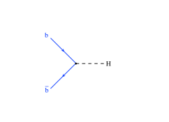
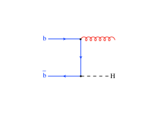
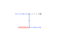
(a)	(b)	(c)

Figure 1: Leading-order (a) and next-to-leading order (b-c) contributions to the hard cross-section in the five-flavor scheme. To order ${\cal O}(\alpha_{s}^{2})$ these processes receive 2-loop corrections (a) and 1-loop corrections (b) and (c), respectively.

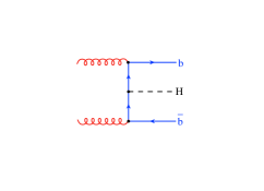
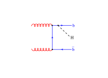
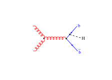
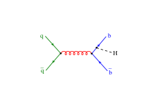
Figure 2: Leading-order order contributions to the four-flavor scheme. Not shown are diagrams that can be obtained by crossing the initial state gluons, or radiating the Higgs off an anti bottom quark.

We now work out Eq. (14) explicitly for Higgs production in bottom-quark fusion, in the simplest FONLL-A case. To NNLL, the partonic cross-section must be computed up to order ${\cal O}(\alpha_{s}^{2})$: it then receives contributions from the following sub-processes:

• ${\cal O}(1)\Rightarrow b\bar{b}\rightarrow h$

• ${\cal O}(\alpha_{s})\Rightarrow b\bar{b}\rightarrow h$ (1-loop), $bg\rightarrow hb$, $b\bar{b}\rightarrow hg$

• ${\cal O}(\alpha_{s}^{2})\Rightarrow b\bar{b}\rightarrow h$ (2-loop), $bg\rightarrow hb$ (1-loop), $b\bar{b}\rightarrow hg$ (1-loop), $bq\rightarrow hbq$, $gg\rightarrow hb\bar{b}$, $bb\rightarrow hb\bar{b}$, $q\bar{q}\rightarrow hb\bar{b}$.

The LO diagrams are shown in Fig. 1. The full calculation up to ${\cal O}(\alpha_{s}^{2})$ can be found in Ref. [15]. The relevant perturbative orders in each parton channel are thus

$$\hat{\sigma}_{b\bar{b}}^{(5)}\left(x_{1},x_{2},\alpha_{s}^{(5)}(\mu^{2})\right) =\hat{\sigma}_{b\bar{b}}^{(5),(0)}(x_{1},x_{2})+\alpha_{s}^{(5)}(\mu^{2})\hat{\sigma}_{b\bar{b}}^{(5),(1)}(x_{1},x_{2})$$

$$+\left(\alpha_{s}^{(5)}(\mu^{2})\right)^{2}\hat{\sigma}_{b\bar{b}}^{(5),(2)}(x_{1},x_{2})+{\cal O}(\alpha_{s}^{3}),$$ (15)

$$\hat{\sigma}_{bg}^{(5)}\left(x_{1},x_{2},\alpha_{s}^{(5)}(\mu^{2})\right) =\alpha_{s}^{(5)}(\mu^{2})\hat{\sigma}_{bg}^{(5),(1)}(x_{1},x_{2})$$

$$+\left(\alpha_{s}^{(5)}(\mu^{2})\right)^{2}\hat{\sigma}_{bg}^{(5),(2)}(x_{1},x_{2})+{\cal O}(\alpha_{s}^{3}),$$ (16)

$$\hat{\sigma}_{bq}^{(5)}\left(x_{1},x_{2},\alpha_{s}^{(5)}(\mu^{2})\right)=\left(\alpha_{s}^{(5)}(\mu^{2})\right)^{2}\hat{\sigma}_{bq}^{(5),(2)}(x_{1},x_{2})+{\cal O}(\alpha_{s}^{3}),$$ (17)

$$\hat{\sigma}_{gg}^{(5)}\left(x_{1},x_{2},\alpha_{s}^{(5)}(\mu^{2})\right)=\left(\alpha_{s}^{(5)}(\mu^{2})\right)^{2}\hat{\sigma}_{gg}^{(5),(2)}(x_{1},x_{2})+{\cal O}(\alpha_{s}^{3}),$$ (18)

$$\hat{\sigma}_{bb}^{(5)}\left(x_{1},x_{2},\alpha_{s}^{(5)}(\mu^{2})\right)=\left(\alpha_{s}^{(5)}(\mu^{2})\right)^{2}\hat{\sigma}_{bb}^{(5),(2)}(x_{1},x_{2})+{\cal O}(\alpha_{s}^{3}),$$ (19)

and

$$\hat{\sigma}_{q\bar{q}}^{(5)}\left(x_{1},x_{2},\alpha_{s}^{(5)}(\mu^{2})\right)=\left(\alpha_{s}^{(5)}(\mu^{2})\right)^{2}\hat{\sigma}_{q\bar{q}}^{(5),(2)}(x_{1},x_{2})+{\cal O}(\alpha_{s}^{3}).$$ (20)

In the four-flavor scheme, the LO ${\cal O}(\alpha_{s}^{2})$ result corresponds to the $gg\rightarrow hb\bar{b}$ and $q\bar{q}\rightarrow hb\bar{b}$ sub-processes shown in Fig. 2. The computation of this process in the four-flavor scheme is formally identical to that of associate production of a Higgs boson with a $t\bar{t}$ pair, first performed in Ref. [1].

We can now match the two expressions. First, we note that in the FONLL-A scheme the four-flavor scheme result is included to lowest nontrivial order: therefore, we can simply replace in it $\alpha_{s}^{(4)}$ and $f_{i}^{(4)}$ with their five-flavor scheme counterparts, as the difference is higher order in $\alpha_{s}$ and thus subleading. We thus simply have

$$B_{ij}\left(x_{1},x_{2},\frac{\mu^{2}}{m^{2}_{b}},\alpha_{s}(\mu^{2})\right)=\hat{\sigma}_{ij}^{(4)}\left(x_{1},x_{2},\frac{\mu^{2}}{m^{2}_{b}},\alpha_{s}(\mu^{2})\right)+{\cal O}(\alpha_{s}^{3}).$$ (21)

We also need the massless limit of the four-flavor scheme result: recalling that it starts at order $\alpha_{s}^{2}$, and using the general expressions Eqs. (11)-(12), we conclude that it must have the form

$$B_{ij}^{(0)}(x_{1},x_{2},L,\alpha_{s} =\left(\alpha_{s}\right)^{2}B_{ij}^{(0),(2)}\left(x_{1},x_{2},L\right)+{\cal O}(\alpha_{s}^{3})$$

$$=\left(\alpha_{s}\right)^{2}\left(A_{ij}^{(2),(0)}(x_{1},x_{2})+A_{ij}^{(1),(1)}(x_{1},x_{2})L+A_{ij}^{(0),(2)}(x_{1},x_{2})L^{2}\right)+{\cal O}(\alpha_{s}^{3}).$$ (22)

The easiest way of determining the coefficients $A_{ij}^{(p),(k)}$ is to start with the five-flavor scheme expression Eq. (1) and expand the bottom PDF in power of $\alpha_{s}$,

$$f_{b}(x,\mu^{2})=\frac{\alpha_{s}(\mu^{2})}{2\pi}L\int_{x}^{1}\frac{dy}{y}P_{qg}(y)f_{g}\left(\frac{x}{y},\mu^{2}\right)+{\cal O}(\alpha_{s}^{2}),$$ (23)

where

$$P_{qg}(y)=T_{R}\left[y^{2}+(1-y)^{2}\right].$$ (24)

We get

$$A_{qq}^{(2),(0)}(x_{1},x_{2}) =\hat{\sigma}_{q\bar{q}}^{(5),(2)}(x_{1},x_{2}),$$ (25)

$$A_{gg}^{(2),(0)}(x_{1},x_{2}) =\hat{\sigma}_{gg}^{(5),(2)}(x_{1},x_{2}),$$ (26)

$$A_{gg}^{(1),(1)}(x_{1},x_{2}) =\frac{1}{2\pi}\int_{0}^{1}dyP_{qg}(y)\left(\hat{\sigma}_{gb}^{(5),(1)}(x_{1},yx_{2})+\hat{\sigma}_{bg}^{(5),(1)}(yx_{1},x_{2})\right)+(b\rightarrow\bar{b}),$$ (27)

$$A_{gg}^{(0),(2)}(x_{1},x_{2}) =\frac{1}{(2\pi)^{2}}\int_{0}^{1}\int_{0}^{1}dy_{1}dy_{2}P_{qg}(y_{1})P_{qg}(y_{2})\hat{\sigma}_{b\bar{b}}^{(5),(0)}(y_{1}x_{1},y_{2}x_{2})+(b\rightarrow\bar{b}),$$ (28)

so that

$$B_{ij}^{(0),(2)}\left(x_{1},x_{2},L,\alpha_{s}\right)=A_{ij}^{(2),(0)}(x_{1},x_{2})+A_{ij}^{(1),(1)}(x_{1},x_{2})L+A_{ij}^{(0),(2)}(x_{1},x_{2})L^{2}.$$ (29)

We now have all the ingredients which enter the FONLL-A expression. For book-keeping purposes, we introduce a formal expansion of the cross-section of the form

$$\sigma^{\rm FONLL-A}=\sigma^{\rm FONLL-A,(0)}+\alpha_{s}(\mu^{2})\sigma^{\rm FONLL-A,(1)}+\left(\alpha_{s}(\mu^{2})\right)^{2}\sigma^{\rm FONLL-A,(2)}+{\cal O}(\alpha_{s}^{3}),$$ (30)

where it is understood that only the coefficient functions $B_{ij}^{(4)}$, $A_{ij}^{(5)}$ and $B_{ij}^{(0)}$ in Eqs. (6), (7) and (12) respectively are expanded, but not the PDFs. The expansion is formal in that, as we have just seen, the nominally ${\cal O}(\alpha_{s}^{0})$ contribution really starts at ${\cal O}(\alpha_{s}^{2})$ once one substitutes the explicit expression Eq. (23) of the $b$-quark distribution, as it should be in order for it to match the four-flavor scheme expression.

Be that as it may, since the four-flavor scheme starts at ${\cal O}(\alpha_{s}^{2})$, $\sigma^{\rm FONLL-A,\{(0),(1)\}}$, the first two terms in the expansion Eq. (30) coincide with the five-flavor scheme expressions:

$$\sigma^{\rm FONLL-A,(0)}=\iint dx_{1}dx_{2}f_{b}(x_{1},\mu^{2})f_{\bar{b}}(x_{2},\mu^{2})\hat{\sigma}_{b\bar{b}}^{(5),(0)}\left(x_{1},x_{2}\right)$$ (31)

$$\sigma^{\rm FONLL-A,(1)} =\iint dx_{1}dx_{2}\left\{f_{b}(x_{1},\mu^{2})f_{\bar{b}}(x_{2},\mu^{2})\hat{\sigma}_{b\bar{b}}^{(5),(1)}\left(x_{1},x_{2}\right)\right.$$

$$\left.+\hat{\sigma}_{gb}^{(5),(1)}(x_{1},x_{2})\left[\left(f_{g}(x_{1},\mu^{2})f_{b}(x_{2},\mu^{2})+(x_{1}\rightarrow x_{2})\right)+(b\rightarrow\bar{b})\right]\right\}.$$ (32)

The ${\cal O}(\alpha_{s}^{2})$ contribution can be written as the sum of two terms: four-flavor scheme, and difference between the five-flavor and the massless limit of the four-flavor scheme. The former is simply given by the leading-order partonic cross-section in the four-flavor scheme.The latter is given by

$$\sigma^{\rm FONLL-A,(2)}=\sigma^{(4),(2)}+\sigma^{(d),(2)},$$ (33)

where

$$\sigma^{(d),(2)}=\sigma^{(5),(2)}-\sigma^{(4),(0),(2)},$$ (34)

and

$$\sigma^{(4),(0),(2)}=\iint dx_{1}dx_{2}\sum_{ij=q,g}f_{i}(x_{1},\mu^{2})f_{j}(x_{2},\mu^{2})B_{ij}^{(0),(2)}\left(x_{1},x_{2},L,\alpha_{s}\right).$$ (35)

We get

$$\sigma^{(d),(2)} =\iint dx_{1}dx_{2}\left\{\vphantom{\sum_{k}^{P}}f_{b}(x_{1},\mu^{2})f_{\bar{b}}(x_{2},\mu^{2})\hat{\sigma}_{b\bar{b}}^{(5),(2)}(x_{1},x_{2})\quad+\right.$$

$$+f_{b}(x_{1},\mu^{2})f_{b}(x_{2},\mu^{2})\hat{\sigma}_{bb}^{(5),(2)}(x_{1},x_{2})\quad+$$

$$+\hat{\sigma}_{gb}^{(5),(2)}(x_{1},x_{2})\left[\left(f_{g}(x_{1},\mu^{2})f_{b}(x_{2},\mu^{2})+(x_{1}\rightarrow x_{2})\right)+(b\rightarrow\bar{b})\right]\quad+$$

$$+\hat{\sigma}_{qb}^{(5),(2)}(x_{1},x_{2})\left[\left(f_{q}(x_{1},\mu^{2})f_{b}(x_{2},\mu^{2})+(x_{1}\rightarrow x_{2})\right)+(b\rightarrow\bar{b},q\rightarrow\bar{q})\right]\quad+$$

$$-\frac{L}{2\pi}\iint dyP_{qg}(y)\left[\vphantom{\sum_{k}}\hat{\sigma}_{bg}^{(5),(1)}(x_{1},yx_{2})\,f_{g}(x_{1},\mu^{2})f_{g}(x_{2},\mu^{2})\right.$$

$$\left.\qquad\qquad+\hat{\sigma}_{bg}^{(5),(1)}(yx_{1},x_{2})f_{g}(x_{1},\mu^{2})f_{g}(x_{2},\mu^{2})+(b\rightarrow\bar{b})\vphantom{\sum_{k}}\right]\quad+$$

$$-\left.\frac{L^{2}}{4\pi^{2}}\iint dy_{1}dy_{2}P_{qg}(y_{1})P_{qg}(y_{2})f_{g}(x_{1},\mu^{2})f_{g}(x_{2},\mu^{2})\hat{\sigma}_{b\bar{b}}^{(5),(0)}(y_{1}x_{1},y_{2}x_{2})\vphantom{\sum_{k}^{P}}\right\},$$ (36)

which is our main result. Note that in the general case in which $\mu_{R}\not=\mu_{F}$, the expansion Eq. (30) should be viewed as an expansion in powers of $\alpha_{s}(\mu_{R})$; the log is $L\equiv\ln\frac{\mu_{F}^{2}}{m_{b}^{2}}$; all PDF should be evaluated at $\mu=\mu_{F}$, and all five-flavor scheme partonic cross-sections should be evaluated at the appropriate scale $\hat{\sigma}_{ij}^{(5),(i)}=\hat{\sigma}_{ij}^{(5),(i)}(\mu^{2}_{R},\mu^{2}_{F})$. Strictly speaking, in this case the argument of the strong coupling in the term in Eq. (S0.Ex5) which is linear in $L$ should be $\alpha_{s}(\mu_{R})\alpha_{s}(\mu_{F})=(\alpha_{s}(\mu_{R}))^{2}(1+O(\alpha_{s}^{3}))$.

It is easy to see explicitly that, if the $b$-PDF is expressed in terms of its values at $\mu^{2}=m_{b}^{2}$ using Eq. (23), the FONLL-A expression differs from the four-flavor scheme result by terms of order $\alpha_{s}^{3}$, namely, the difference term

$$\sigma^{(d)}=\sigma^{(5),(0)}+\alpha_{s}(\mu^{2})\sigma^{(5),(1)}+(\alpha_{s}(\mu^{2}))^{2}\sigma^{(d),(2)}$$ (37)

is ${\cal O}(\alpha_{s}^{3})$. Indeed, Eq. (23) implies that all contributions to $\sigma^{(d),(2)}$ but the logarithmic ones are ${\cal O}(\alpha_{s}^{3})$. We then have

$$\sigma^{(d)} =\iint dx_{1}dx_{2}\Bigg{\{}\Big{[}f_{b}(x_{1},\mu^{2})f_{\bar{b}}(x_{2},\mu^{2})\hat{\sigma}_{b\bar{b}}^{(5),(0)}\left(x_{1},x_{2}\right)$$

$$-\frac{\alpha_{s}^{2}L^{2}}{4\pi^{2}}\iint dy_{1}dy_{2}P_{qg}(y_{1})P_{qg}(y_{2})f_{g}(x_{1},\mu^{2})f_{g}(x_{2},\mu^{2})\hat{\sigma}_{b\bar{b}}^{(5),(0)}(y_{1}x_{1},y_{2}x_{2})\Big{]}$$ (38)

$$+\Big{[}\alpha_{s}\hat{\sigma}_{gb}^{(5),(1)}(x_{1},x_{2})\left(f_{g}(x_{1},\mu^{2})f_{b}(x_{2},\mu^{2})+(x_{1}\rightarrow x_{2})\right)$$

$$-\frac{\alpha_{s}^{2}L}{2\pi}\int dyP_{qg}(y)\left(\hat{\sigma}_{bg}^{(5),(1)}(x_{1},yx_{2})\,+\hat{\sigma}_{bg}^{(5),(1)}(yx_{1},x_{2})\right)f_{g}(x_{1},\mu^{2})f_{g}(x_{2},\mu^{2})\Big{]}\Bigg{\}}\,+\,{\cal O}(\alpha_{s}^{3}).$$

Substituting Eq. (23) in Eq. (38) all terms in Eq. (38) cancel, as expected.

We can now study the phenomenological implications of our results. Leading-order four-flavor scheme predictions have been obtained using a modified version of the SHERPA Monte Carlo generator [21] which we tested against results obtained in Ref. [16] and Ref. [22]; for NLO results (which we will also show for comparison) this has been further interfaced to the OpenLoops code [23]. Four-flavor scheme results are obtained using $n_{f}=4$ NNPDF3.0 LO PDFs [24] with $\alpha^{\rm 5F}_{S}(m_{Z})=0.118$. Five-flavor scheme predictions are obtained using the bbh@nnlo code [15] with the $n_{f}=5$ NNLO NNPDF3.0 parton set [24]. For FONLL-A, results for the central scale choice have been obtained in two different ways. First, we have recomputed the four-flavor scheme result, but now using $n_{f}=5$ NNLO NNPDF3.0 PDFs, and we have combined this with our implementation of Eq. (S0.Ex5). Then, we have checked that we get the same answer by combining this four-flavor scheme result with the five-flavor scheme one from the bbh@nnlo code, and adding an implementation of the subtraction term Eq. (13). Scale variation plots have then been produced using this second combination. In all cases, the strong coupling provided with the PDF set has been used through the LHAPDF interface [25]. The $b$ mass in FONLL expressions has been identified with the pole mass, for which we have taken the value $m_{b}=4.72$ GeV; this corresponds to the $\overline{\rm MS}$ value $\overline{m}_{b}(\overline{m}_{b})=4.21$ GeV through the two-loop relation of Ref. [26], which we implemented in order to evaluate the bottom Yukawa coupling in the $\overline{\text{MS}}$ scheme at $\mu=\mu_{R}$. Like $\alpha_{s}$ and the PDFs, Yukawa couplings are evolved at NNLO in the five-flavor scheme in all contributions to the FONLL expression.

In Fig. 3 we compare the cross-section computed in the four-flavor, five-flavor and FONLL-A scheme. Results are shown as a function of the Higgs mass. Here and henceforth, uncertainty bands are obtained by varying the renormalization and factorization scales $\mu_{R}$ and $\mu_{F}$ independently by a factor of 2 about the central value $\mu_{F}=\mu_{R}=m_{H}$, discarding the two extreme points $\mu_{R}=4\mu_{F}$ and $\mu_{F}=4\mu_{R}$, and taking the envelope of results. In the same figure we also show the curve obtained using the so-called Santander matching of Ref. [11], which is given by

$$\sigma_{S-M}=\frac{\sigma^{(4F)}+w\,\sigma^{(5F)}}{1+w}\,.$$ (39)

with $w=\ln{m_{H}/m_{b}}-2$: this reproduces the five-flavor scheme result when $w\to\infty$, and the four-flavor scheme one when $w=0$. This prescription was suggested in Ref. [11] to be used with the highest-order available four- and five-flavor scheme results. Here, we show it using the LO four-flavor scheme result in order to provide a meaningful assessment of the differences in comparison to FONLL-A.

Figure 3: The total inclusive cross-section computed in the four-flavor scheme at LO (red), in the five-flavor scheme at NNLO (blue), and in the FONLL-A scheme (green). The Santander matching Eq. 39 of the four and five-flavor scheme results is also shown (purple). Both the absolute result (top) and the ration to the FONLL-A prediction (bottom) are shown.

The four-flavor scheme result is rather smaller than the five-flavor scheme one, and it is affected by a significantly larger scale uncertainty, as one expects of a LO computation. The FONLL and five-flavor scheme results are very close, with, for $m_{h}=125.09$ GeV, the FONLL prediction just below the five-flavor one, with a somewhat larger uncertainty. Note that the four-flavor scheme result shown in the plot is determined using LO PDFs, while the four-flavor scheme result that enters the FONLL combination is consistently computed with NNLO PDFs, as discussed above. We have verified that the latter would be yet lower, further away from the five-flavor scheme results, as one expects due to the fact the the LO gluon is typically larger. This shows that mass effects for this process are small, though not negligible in comparison to the scale uncertainty on the five-flavor result, as we will see shortly. The fact that mass-corrections at leading order are small was already noticed in Ref. [27]. Such a quantitative conclusion cannot be arrived at using the Santander-matched result, which simply interpolates between the four- and five-flavor scheme results.

The scale dependence of the various results of Fig. 3 is shown in Fig. 4 for $m_{H}=125.09$ GeV. The four- and five-flavor scheme results display a significant renormalization scale dependence. The four-flavor scheme result drops significantly as the scale is increased because of the reduction in value of $\alpha_{s}$, while the five-flavor scheme results grows because the residual, weaker $O(\alpha_{s}^{3})$ dependence has the opposite sign (NNLO corrections are negative) combines with the growth of the Yukawa coupling with scale. Interestingly, this scale dependence cancels to a large extent both in the FONLL-A and Santander matched results. As a consequence, the mass-corrections included in the FONLL-A result, and the scale dependence of the five-flavor scheme computation are of comparable size, with the FONLL result below the massless one at the upper range of the scale variation, and above it for lower scale choices, and specifically if the renormalization scale is fixed at $\mu_{R}=\frac{m_{H}+2m_{b}}{4}$, as recommended in Refs. [16, 8, 28], with a crossing point just below $\mu_{R}=m_{H}$.

The factorization scale dependence is very mild in all schemes, except for FONLL, where it turns out that the scale dependence is of the same order as the mass-corrections, which as we have seen are small but not negligible. In fact, the factorization scheme dependence shown in the plot has been determined using as argument of the strong coupling for the term in Eq. (S0.Ex5) which is linear in $L$ $\alpha_{s}(\mu_{R})\alpha(\mu_{F})$, as discussed above. If one makes the choice $(\alpha_{s}(\mu_{R})^{2})$, which is equivalent up to subleading term, the scale dependence changes (and in fact it becomes stronger) by an amount which is comparable to the scale variation itself. This means that corrections of relative order $(\alpha_{s}(\mu_{R})^{2})\ln(\mu_{R}/\mu_{F})$ to the mass-corrections are not negligible on the scale of the mass-corrections themselves. They could only be accounted for by upgrading the four-flavor scheme computation to NLO.

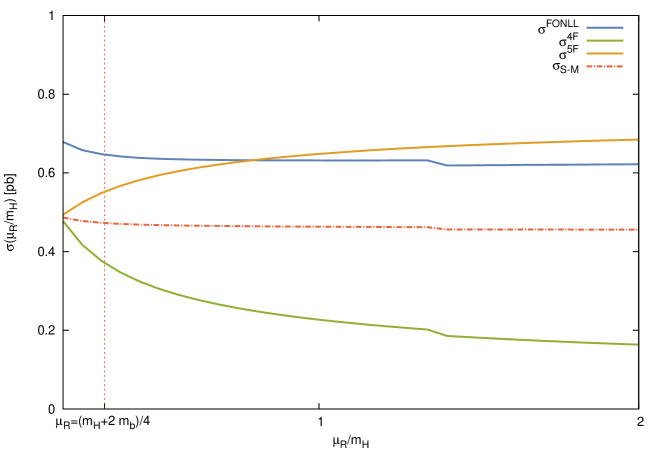
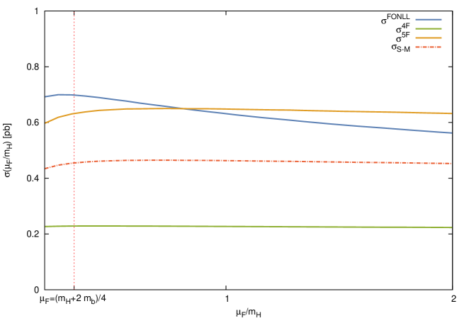
Figure 4: Renormalization (top) and factorization (bottom) scale dependence of the cross-sections shown in Fig. 3 with $m_{H}=125.09$ GeV. The preferred scale choice $\frac{m_{H}+2m_{b}}{4}$ is denoted by a vertical bar.

Finally, in Table 1 we collect our results with $m_{H}=125.09$ GeV and $\mu=m_{H}$ or $\mu=\frac{m_{H}+2m_{b}}{4}$. For comparison, in addition to the results shown in Figs. 3-4 we also show the best available calculation in the four-flavor scheme (NLO) and its Santander matching to the NNLO five-flavor result.

	$\sigma^{\rm(5F)}$ (pb)	$\sigma_{\rm LO}^{\rm(4F)}$ (pb)	$\sigma^{\rm FONLL}$ (pb)	$\sigma_{A}^{\rm S-M}$ (pb)	$\sigma^{\rm(4F)}$ (pb)	$\sigma^{\rm S-M}$
$\mu=m_{H}$	$0.65_{-0.03}^{+0.07}$	$0.22^{+0.25}_{-0.06}$	$0.63_{-0.01}^{+0.34}$	$0.55^{+0.20}_{-0.10}$	$0.26_{-0.10}^{+0.19}$	$0.56_{-0.13}^{+0.12}$
$\mu=(m_{H}+2m_{b})/4$	$0.61$	$0.41$	$0.82$	$0.56$	$0.42$	$0.57$

Table 1: The total cross-section computed for $m_{H}=125.09$ GeV in the five-flavor scheme at NNLO, the four-flavor scheme at LO, and matching the two with FONLL-A, or with Santander matching (denoted as $\sigma_{A}^{\rm S-M}$). The NLO four-flavor scheme result, and its Santander matching to the five-flavor scheme are also shown for comparisons. Results are given for $\mu=m_{H}$ (top row) and $\mu=(m_{H}+2m_{b})/4$ (bottom row). For $\mu=m_{H}$ we also show the uncertainty band obtained from scale variation (see text).

In summary, we have shown how to consistently match the four- and five-flavor scheme computations of Higgs production in bottom-quark fusion. We have found that a fully matched computation allows detailed quantitative comparisons between the computations in various schemes, unlike other more phenomenological approaches. However, for competitive precision phenomenology, the results presented in this paper should be upgraded to include the four-flavor scheme result up to NLO: indeed, the factorization scheme dependence of the mass corrections turns out to be comparable to their size. Such an upgrade is possible by using the scheme presented here, in its FONLL-B version, which requires an in principle straightforward, though in practice somewhat laborious extension of the techniques presented in this paper: this is the object of ongoing work.

References

[1]
Z. Kunszt, Associated Production of Heavy Higgs Boson with Top Quarks,
Nucl. Phys.B247 (1984) 339.
[2]
D. A. Dicus and S. Willenbrock, Higgs Boson Production from Heavy Quark
Fusion, Phys. Rev.D39 (1989) 751.
[3]
R. M. Barnett, H. E. Haber, and D. E. Soper, Ultraheavy Particle
Production from Heavy Partons at Hadron Colliders, Nucl. Phys.B306 (1988) 697.
[4]
D. Dicus, T. Stelzer, Z. Sullivan, and S. Willenbrock, Higgs boson
production in association with bottom quarks at next-to-leading order,
Phys. Rev.D59 (1999) 094016,
[hep-ph/9811492].
[5]
M. Spira, Higgs boson production and decay at the Tevatron, in Physics at Run II: Workshop on Supersymmetry / Higgs: Summary Meeting
Batavia, Illinois, November 19-21, 1998, 1998.
hep-ph/9810289.
[6]
D. L. Rainwater, M. Spira, and D. Zeppenfeld, Higgs boson production at
hadron colliders: Signal and background processes, in Physics at TeV
colliders. Proceedings, Euro Summer School, Les Houches, France, May 21-June
1, 2001, 2002.
hep-ph/0203187.
[7]
T. Plehn, Charged Higgs boson production in bottom gluon fusion, Phys. Rev.D67 (2003) 014018,
[hep-ph/0206121].
[8]
F. Maltoni, Z. Sullivan, and S. Willenbrock, Higgs-boson production via
bottom-quark fusion, Phys. Rev.D67 (2003) 093005,
[hep-ph/0301033].
[9]
F. Maltoni, G. Ridolfi, and M. Ubiali, b-initiated processes at the LHC:
a reappraisal, JHEP07 (2012) 022,
[arXiv:1203.6393]. [Erratum:
JHEP04,095(2013)].
[10]
M. Ubiali, Are bottom PDFs needed at the LHC?, PoSDIS2014
(2014) 037.
[11]
R. Harlander, M. Kramer, and M. Schumacher, Bottom-quark associated
Higgs-boson production: reconciling the four- and five-flavour scheme
approach, arXiv:1112.3478.
[12]
M. Cacciari, M. Greco, and P. Nason, The P(T) spectrum in heavy flavor
hadroproduction, JHEP05 (1998) 007,
[hep-ph/9803400].
[13]
S. Forte, E. Laenen, P. Nason, and J. Rojo, Heavy quarks in
deep-inelastic scattering, Nucl. Phys.B834 (2010) 116–162,
[arXiv:1001.2312].
[14]
S. J. Brodsky, P. Hoyer, C. Peterson, and N. Sakai, The Intrinsic Charm
of the Proton, Phys. Lett.B93 (1980) 451–455.
[15]
R. V. Harlander and W. B. Kilgore, Higgs boson production in bottom quark
fusion at next-to-next-to leading order, Phys. Rev.D68 (2003)
013001, [hep-ph/0304035].
[16]
S. Dittmaier, M. Kramer, 1, and M. Spira, Higgs radiation off bottom
quarks at the Tevatron and the CERN LHC, Phys. Rev.D70 (2004)
074010, [hep-ph/0309204].
[17]
S. Dawson, C. B. Jackson, L. Reina, and D. Wackeroth, Exclusive Higgs
boson production with bottom quarks at hadron colliders, Phys. Rev.D69 (2004) 074027, [hep-ph/0311067].
[18]
T. Han, J. Sayre, and S. Westhoff, Top-Quark Initiated Processes at
High-Energy Hadron Colliders, JHEP04 (2015) 145,
[arXiv:1411.2588].
[19]
M. A. G. Aivazis, J. C. Collins, F. I. Olness, and W.-K. Tung, Leptoproduction of heavy quarks. 2. A Unified QCD formulation of charged and
neutral current processes from fixed target to collider energies, Phys. Rev.D50 (1994) 3102–3118,
[hep-ph/9312319].
[20]
J. Rojo et al., “Chapter 22 in: J. R. Andersen et al., The SM and NLO
multileg working group: Summary report.” arXiv:1003.1241, 2010.
[21]
T. Gleisberg, S. Hoeche, F. Krauss, M. Schonherr, S. Schumann, F. Siegert, and
J. Winter, Event generation with SHERPA 1.1, JHEP02
(2009) 007, [arXiv:0811.4622].
[22]
M. Wiesemann, R. Frederix, S. Frixione, V. Hirschi, F. Maltoni, and
P. Torrielli, Higgs production in association with bottom quarks,
JHEP02 (2015) 132,
[arXiv:1409.5301].
[23]
F. Cascioli, P. Maierhofer, and S. Pozzorini, Scattering Amplitudes with
Open Loops, Phys. Rev. Lett.108 (2012) 111601,
[arXiv:1111.5206].
[24]NNPDF Collaboration, R. D. Ball et al., Parton distributions for
the LHC Run II, JHEP04 (2015) 040,
[arXiv:1410.8849].
[25]
A. Buckley, J. Ferrando, S. Lloyd, K. Nordström, B. Page, M. Rüfenacht,
M. Schönherr, and G. Watt, LHAPDF6: parton density access in the LHC
precision era, Eur. Phys. J.C75 (2015), no. 3 132,
[arXiv:1412.7420].
[26]
J. H. Kuhn, M. Steinhauser, and C. Sturm, Heavy Quark Masses from Sum
Rules in Four-Loop Approximation, Nucl. Phys.B778 (2007)
192–215, [hep-ph/0702103].
[27]
C. Buttar et al., Sect. 24 in: Les houches physics at TeV colliders 2005,
standard model and Higgs working group: Summary report, in Physics
at TeV colliders. Proceedings, Workshop, Les Houches, France, May 2-20,
2005, 2006.
hep-ph/0604120.
[28]LHC Higgs Cross Section Working Group Collaboration, S. Dittmaier et al.,
Handbook of LHC Higgs Cross Sections: 1. Inclusive Observables,
arXiv:1101.0593.