First-order phase transition and tricritical point in multiband $U(1)$ London superconductors

Abstract

The order of the superconducting phase transition is a classical problem. Single-component type-2 superconductors exhibit a continuous “inverted-XY” phase transition, as was first demonstrated for $U(1)$ lattice London superconductors by a celebrated duality mapping with subsequent backing by numerical simulations. Here we study this problem in multiband $U(1)$ London superconductors and find evidence that by contrast the model has a tricritical point. The superconducting phase transition becomes first-order when the Josephson length is sufficiently large compared to the magnetic field penetration length. We present evidence that the fluctuation-induced dipolar interaction between vortex loops makes the phase transition discontinuous. We discuss that this mechanism is also relevant for the phase transitions in multicomponent gauge theories with higher broken symmetry.

The problem of the order of the superconducting phase transition beyond mean-field approximation is more than 40 years old. In Halperin et al. (1974) it was observed that if phase fluctuations are neglected in the Ginzburg-Landau model, fluctuations of the vector potential make the superconducting phase transition first-order (see also Coleman and Weinberg (1973)). This scenario applies only for strongly type-1 superconductors, as was demonstrated by later works Thomas and Stone (1978); Peskin (1978); Dasgupta and Halperin (1981). These works considered a lattice London model, neglecting fluctuations of the modulus of the order parameter but taking into account phase fluctuations. It was demonstrated that the superconducting phase transition beyond mean-field approximation is caused by the proliferation of vortex loops with short-range interaction set by the magnetic field penetration length $\lambda$. For low temperatures only small vortex rings are thermally excited, while at $T_{c}$ the thermally excited vortex loops loose their line tension and extend throughout the entire system.

In Refs. Thomas and Stone (1978); Peskin (1978); Dasgupta and Halperin (1981) a duality mapping was established between the statistical problem of the normal state above $T_{c}$ in a superconductor and a statistical description of a superfluid state below $T_{c}$, such that the temperature axis is reversed, see also Olsson and Teitel (1998). Thus the phase transition in the lattice London superconductor is called the “inverted-3D XY” transition. The London limit approximation is justifiable for extreme type-2 superconductors. The question at what parameter values of the Ginzburg-Landau model the inverted-3D XY phase transition turns into first-order has subsequently been studied using various approaches. Some of the attempted analytical approaches Kleinert (1982) suggested that the continuous phase transition extends slightly into the region where the Ginzburg-Landau parameter $\kappa$ is smaller than $1$ (or, equivalently, in traditional units smaller than $1/\sqrt{2}$). However this approach was based on uncontrollable assumptions, and thus numerical simulations were required to address that question. Early numerical work were consistent with the existence of a tricritical point Bartholomew (1983), as well as one-loop renormalization-group calculations Herbut and Tešanović (1996). The largest-scale Monte Carlo simulation performed so far Mo et al. (2002) suggests that the continuous phase transition indeed extends slightly into the region of $\kappa<1$. All these works suggested that in London model (which corresponds to taking extremely type-2 limit) the phase transition is continuous.

Recently there has been a surge of interest to multicomponent $U(1)\times U(1)$ and $SU(2)$ generalizations of this problem in the context of multicomponent superconducting condensates Babaev (2004); Babaev et al. (2004); Herland et al. (2010) and of deconfined quantum criticality proposals where such Ginzburg-Landau models were argued to arise as an effective field theory Motrunich and Vishwanath (2004); Senthil et al. (2004); Sachdev (2008); Chen et al. (2013). Initially it was suggested that $SU(2)$ as well as $U(1)\times U(1)$ superconductors with equal phase stiffnesses possess a continuous phase transition from a state with fully broken symmetries to a normal state in a novel universality class Senthil et al. (2004); Motrunich and Vishwanath (2004, 2008), but later analysis revealed first-order phase transitions Kuklov et al. (2005, 2008a); Chen et al. (2013); Kuklov et al. (2006); Herland et al. (2010); Kuklov et al. (2008b); Kragset et al. (2006); Herland et al. (2013) in such systems. The flowgram method proposed in Kuklov et al. (2006) shows that the phase transition remains first order in the limit of infinitesimally small electric charge. First-order phase transitions were also found in $U(1)\times Z_{2}$ systems, where a $Z_{2}$ symmetry associated with broken time-reversal symmetry is caused by a frustrated intercomponent coupling Bojesen et al. (2014).

Most of the superconductors which are of great current interest are multiband superconductors Suhl et al. (1959); Moskalenko (1959); Leggett (1966). In the London limit multiband superconductors are described by several phases coupled by a Josephson interaction Leggett (1966). Here we consider the problem of the phase transition in a multi-component London superconductor with condensates $\psi_{a}=|\psi_{a}|\exp(i\theta^{(a)})$ ($a=1,2,...$), with constant $|\psi_{a}|$, described by the free-energy density

$$f= \frac{1}{2}\sum_{a}|\psi_{a}|^{2}(\nabla\theta^{(a)}+e\mathbf{A})^{2}+\frac{1}{2}\left(\nabla\times\mathbf{A}\right)^{2}$$

$$-\sum_{a>b}\eta_{ab}|\psi_{a}||\psi_{b}|\cos(\theta^{(a)}-\theta^{(b)}),$$ (1)

where $e$ is the electric charge coupling and $\eta_{ab}$ determines the strength of the Josephson phase-difference-locking term between bands $a$ and $b$. We are interested here in the case where the Josephson coupling breaks the symmetry explicitly to $U(1)$, and to restrict the parameter space we will consider $\eta_{ab}=\eta$. In Smiseth et al. (2005) a duality mapping was discussed for a class of $U(1)$ multi-band models. Namely, it was discussed that the dual version of the model is described by proliferation of a single kind of directed loops. That indicates that if the phase transition is continuous then it should be in the “inverted-3D XY” universality class. However it was established recently that intermediate-length-scale interaction in the directed-loops model can make the phase transition first-order Meier et al. (2015). Thus the origin of the phase transition in multi-band models requires a careful study.

We begin by examining the two-band case, then without loss of generality $\eta$ can be taken to be non-negative, such that in the ground state $\theta^{(1)}-\theta^{(2)}=0$. From the free energy two characteristic length scales can be identified: the first one is the London magnetic penetration depth $\lambda$ and the second one is the Josephson length $\xi_{J}$, the latter at which the system restores the ground state from small deviations in the phase difference. As previously mentioned, the London model is justified for strongly type-2 multiband superconductors, where the coherence lengths associated with the densities are much smaller than $\lambda$ and $\xi_{J}$. The Josephson length $\xi_{J}$ can be identified by writing $\theta^{(1)}(x)-\theta^{(2)}(x)=\delta(x)$, imposing the condition $\delta(0)=\delta_{0}$, and expanding the Josephson term. Then the system recovers ground state value of the phase difference according to the exponential law $\delta(x)=\delta_{0}\exp\left(-x/\xi_{J}\right)$ with $\xi_{J}=\sqrt{|\psi_{1}||\psi_{2}|/(\eta(|\psi_{1}|^{2}+|\psi_{2}|^{2}))}$. The standard expression for the magnetic field penetration depth is $\lambda=1/(e\sqrt{|\psi_{1}|^{2}+|\psi_{2}|^{2}})$.

When $\eta=0$, the model has $U(1)\times U(1)$ symmetry. As mentioned above, the phase diagram of such a system have been previously studied, in two dimensions Babaev (2004), three dimensions in an external field Babaev et al. (2004); Smørgrav et al. (2005a, b) and three-dimensional cases without an external field Kuklov et al. (2006); Herland et al. (2010). In three dimensions, at a low but non-zero value of the coupling constant $e$, the model exhibits a single first-order phase transition from the $U(1)\times U(1)$-state to the normal state. For large electric charges there are two phase transitions. The reason for occurrence of the second phase transition is the following: at a lower critical temperature a proliferation of bound states of vortices with winding in both phases takes place: i.e. vortices for which $\Delta\theta^{(1)}\equiv\oint_{\sigma}\nabla\theta^{(1)}=2\pi,\ \Delta\theta^{(2)}\equiv\oint_{\sigma}\nabla\theta^{(2)}=2\pi$ where the integration path $\sigma$ encloses two cores, such vortices are denoted by (1,1). The “elementary” vortices in the individual condensates are bound into these composite objects through the coupling to the vector potential. In the resulting state the individual phases $\theta^{(a)}$ are disordered but the phase difference is ordered Babaev (2004); Babaev et al. (2004); Smørgrav et al. (2005a); Kuklov et al. (2006); Herland et al. (2010). This state is called a metallic superfluid, paired state or super-counter-fluid. At elevated temperatures the transition into the normal state is driven by the proliferation of individual (also termed fractional) vortices $\Delta\theta^{(1)}\equiv\oint_{\sigma}\nabla\theta^{(1)}=2\pi,\ \Delta\theta^{(2)}\equiv\oint_{\sigma}\nabla\theta^{(2)}=0$, denoted by $(1,0)$ and $\Delta\theta^{(1)}\equiv\oint_{\sigma}\nabla\theta^{(1)}=0,\ \Delta\theta^{(2)}\equiv\oint_{\sigma}\nabla\theta^{(2)}=2\pi$, denoted by $(0,1)$. For the properties of the individual and composite vortices in this model see Babaev (2002, 2004).

It has been discussed that the existence of the paired states in multicomponent gauge theories could be related to first-order phase transitions Kuklov et al. (2006). Indeed, even at the level of mean-field analysis the direct $U(1)\times U(1)$ or $SU(2)$ phase transitions are first-order in the vicinity (on the phase diagram) of the paired state. However mean-field analysis is qualitatively wrong for this problem in general, failing to capture first order phase transition happening in the $e\to 0+$ limit. By contrast, the model (1) shares the same symmetry as single-component superconductors, indeed the Josephson coupling breaks the symmetry explicitly to $U(1)$.

By discretizing the model (1) onto a cubic grid of size $L$, rewriting the gradients with finite differences, the kinetic energy terms into XY-model cosines, and inserting the previously identified length scales, we obtain the lattice Hamiltonian for the two-band case

$$H=\sum_{i}\Bigg{[} \sum_{a}\sum_{\mu}-|\psi_{a}|^{2}\cos(\theta^{(a)}_{i+\hat{\mu}}-\theta^{(a)}_{i}+A_{i\mu})$$

$$+\frac{1}{2}\lambda^{2}(|\psi_{1}|^{2}+|\psi_{2}|^{2})\sum_{\mu}[\Delta\times\mathbf{A}]_{i\mu}^{2}+$$

$$-\frac{1}{\xi_{J}^{2}}\frac{|\psi_{1}|^{2}|\psi_{2}|^{2}}{|\psi_{1}|^{2}+|\psi_{2}|^{2}}\cos(\theta^{(1)}_{i}-\theta^{(2)}_{i})\Bigg{]},$$ (2)

where $i$ is a lattice site index, $\mu=x,y,z$ and $[\Delta\times\mathbf{A}]_{i\mu}=A_{i\mu^{\prime}}+A_{i+\hat{\mu}^{\prime},\mu^{\prime\prime}}-A_{i+\hat{\mu}^{\prime\prime},\mu^{\prime}}-A_{i\mu^{\prime\prime}}$ is the discrete lattice curl, where we have denoted $x^{\prime}=y$, $y^{\prime}=z$ and $z^{\prime}=x$. We simulate the temperature-driven phase transitions of the Hamiltonian (2) with a parallel tempering Metropolis Monte Carlo algorithm Swendsen and Wang (1986); Earl and Deem (2005); Newman and Barkema (1999) and use periodic boundary conditions. The trial moves consist of selecting a site at random and proposing new values for all five site degrees of freedom (two phases and three vector potential components). The phases are updated by drawing random numbers between 0 and $2\pi$, and the components of the vector potential are updated by adding (either positive or negative) random numbers to the old values. Parallel tempering swap trial moves between adjacent temperatures are attempted with a fixed frequency Earl and Deem (2005); Manousiouthakis and Deem (1999) of once every sweep. To collect data we perform simulations of at least $10^{6}$ sweeps and we perform the simulations with linearly distributed temperatures.

We begin by determining how a finite Josephson coupling term affects the maximal value of the heat capacity and the corresponding temperature. We consider the case of twin bands $|\psi_{1}|^{2}=|\psi_{2}|^{2}=1$ with $\lambda^{2}=0.2$ and vary $\eta$ over several orders of magnitude. Fig. 1 shows the maximal value of the calculated heat capacity as well as the corresponding temperature, taken to be the critical temperature for two system sizes. Each point on the curves corresponds to a simulation and the lines are guides to the eye (note however that the temperature curves overlap). The simulations have a fixed set of temperatures each, chosen manually to cover the heat capacity peak.

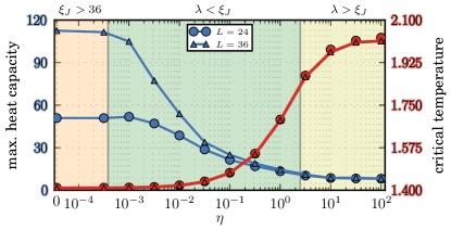
Figure 1: The maximum of the calculated heat capacity (left vertical axis, blue) and its corresponding critical temperature (right vertical axis, red) for $L=24$ (circles) and $L=36$ (triangles), with Josephson coupling $\eta$ varying over several orders of magnitude.

As is seen in Fig. 1, the heat capacity peak is larger in the region where the Josephson interaction is small. As the Josephson interaction is increased, the Josephson length becomes smaller as does the magnitude of the heat capacity peak. In the right-most region where the Josephson length is smaller than the magnetic penetration depth, the magnitude of heat capacity peak is not visibly different for the two system sizes. The critical temperature raises as the heat capacity peak diminishes and is not visibly affected by changing the system size. The behavior of the displayed quantities suggests that the left-most and right-most points of Fig. 1) represents two distinct physical regimes.

For the left-most point in Fig. 1 (with $\eta=0$) the symmetry of the system is $U(1)\times U(1)$, which, as previously mentioned, is known to have a first-order phase transition (Kuklov et al., 2005, 2006; Dahl et al., 2008). This, combined with the observation that the heat capacity maximum grows substantially with the system size in the region of finite and small $\eta$, suggests that the phase transition is of first-order also for finite $\eta$ in the region with $\lambda<\xi_{J}$. In the region of $\lambda>\xi_{J}$ however, any growth in the heat capacity maximum with system size is not visible in Fig. 1, suggesting there is a tricritical point and a continuous phase transition for $\lambda>\xi_{J}$.

We consider first the scaling properties for $\eta=10^{-3}$ (with $\xi_{J}\approx 23$) which is in the $\lambda<\xi_{J}$-region of Fig. 1. The internal energy histogram at the phase transition is seen in Fig. 2 a) to be bimodal, and the bimodality is enhanced by increasing the system size. The free-energy barrier $\Delta F=(\beta_{c})^{-1}\ln(P_{max}/P_{min})$ ($\beta_{c}$ is the inverse critical temperature and $P$ the energy distribution) is seen in Fig. 2 b) to be proportional to $L^{2}$ and the latent heat $\Delta H$ (i.e. the distance between the peaks) is seen in c) to not vanish, indicating a first-order phase transition Lee and Kosterlitz (1990, 1991). By contrast, we observed no bimodal features or tendencies for any system with $\lambda>\xi_{J}$.

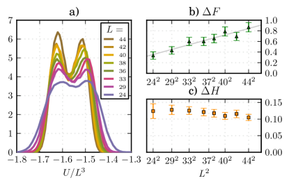
Figure 2: For $\eta=10^{-3}$ the scaling behavior of the energy histograms (normalized distributions of the internal energy per site $U/L^{3}$) at the phase transition is indicative of a first-order phase transition. The histograms for various lattice sizes are shown in a), the free-energy barrier $\Delta F$ is shown in b) and the latent heat $\Delta H$ in c).

We find that when the Josephson interaction is increased, the system size required for a bimodal energy distribution to develop also increases. This makes it computationally difficult to reproduce the scaling results of Fig. 2 for systems where the Josephson length is much smaller than the box length. To further test these phenomena we consider a three- and four-band models with $|\psi_{i}|^{2}=1$ with a Josephson coupling which locks all the phase differences to zero in the ground state. In such a system we find that the first-order phase transition becomes stronger and the measurement of bimodal energy distributions for $\xi_{J}\ll L$ is possible. In Fig. 3 is shown the first-order scaling of the energy histograms for a three-band model with $\eta=0.03$ such that $\xi_{J}\approx 3.3$ up to $L=44$, more that ten Josephson lengths. The results of Fig. 3 are $10^{6}$ sweep simulations with $\lambda^{2}=0.1$. In Fig. 4 is shown simulation results for a four-band model with an even stronger Josephson coupling of $\eta=0.07$, and $\lambda^{2}=0.075$. The four-band results are $2\cdot 10^{6}$ sweep simulations with sampling during the last $500000$ sweeps. With the growing number of components we find stronger signatures of the first order phase transitions.

Figure 3: First-order scaling of the energy histograms for the three-band model also hold when $\xi_{J}\ll L$, here $\xi_{J}=3.3$ with scaling up to $L=44$.

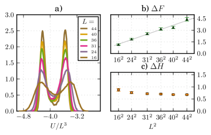
Figure 4: First-order scaling of the energy histograms is more pronounced for a four-band model.

Consider next the scaling properties for the two-band model at the point $\eta=10^{0.5}$ which is in the region of $\lambda>\xi_{J}$ in Fig. 1 (with $\xi_{J}\approx 0.40$). In Fig. 5 it is seen that the energy cumulant $V_{L}=1-\langle U^{4}\rangle/(3\langle U^{2}\rangle^{2})$ has for $\eta=10^{-3}$ a minimum that is persistent against scaling, as it should for a first-order transition Challa et al. (1986). For $\eta=10^{0.5}$ however, the energy cumulant has no distinct minimum, a behavior which is consistent with a continuous phase transition where the energy cumulant reaches the trivial limit of $2/3$ everywhere in the thermodynamic limit. Indeed, in the limit of strong interband coupling the system should recover the standard 3D inverted-XY phase transition like in a single-component model Peskin (1978); Dasgupta and Halperin (1981).

Figure 5: Scaling behavior of the heat capacity (left column) and energy cumulant (right) for $\eta=10^{-3}$ (with $\lambda<\xi_{J}$, blue lines) and $\eta=10^{0.5}$ (with $\lambda>\xi_{J}$, red lines), indicates a first-order and a continuous phase transition respectively. Shaded regions around curves correspond to estimated errors.

We interpret the results as suggestive to an emergent attractive interaction between vortex lines. It has been recently demonstrated that in a single-component directed-loops (${\bf j}$-current) model, a modification of the vortex interaction potential from short-range repulsive to short-range non-monotonic asymptotically attractive, causes a conversion of the inverted-XY transition to a first-order one Meier et al. (2015). The model under consideration here features fluctuation-induced attractive inter-vortex forces. Indeed, if the Josephson coupling is set to zero, a fractional vortex has a logarithmically divergent energy while co-directed individual vortices interact logarithmically at large distances. For a two-dimensional cross-section of a pair of fractional vortices in the two-component model with $|\psi_{1}|^{2}=|\psi_{2}|^{2}=|\psi|^{2}$ and phase winding in the first condensate, the interaction energy Babaev (2002, 2004) is:

$$E^{int}_{(1,0)+(1,0)} = \pi|\psi|^{2}\,\,\log\frac{R}{r}\,+\,\pi\,|\psi|^{2}K_{0}(r/\lambda).$$ (3)

The interaction between $(1,0)$- and $(0,1)$-vortices contains an attractive logarithmic part and a repulsive exponentially screened part:

$$E^{int}_{(1,0)+(0,1)} = -\pi|\psi|^{2}\,\log\frac{R}{r}\,+\,{\pi}|\psi|^{2}K_{0}(r/\lambda).$$ (4)

In the absence of fluctuations, a composite vortex line is an axially symmetric object with finite energy per unit length. The attractive and repulsive forces cancel in the small separation limit Babaev (2002, 2004), however at separations larger than $\lambda$ a pair of co-directed fractional vortices can be mapped onto an electric dipole. Due to the long-range nature of the dipolar interaction, the thermal splitting of composite vortices into fractional vortices will lead to long-range attractive, short-range repulsive interaction. When a non-zero Josephson coupling is included, the interaction between fractional vortices is changed to linearly attractive at distances larger than $\xi_{J}$ Babaev (2002). Then the splitting fluctuations of fractional vortices are largely confined within the range $\xi_{J}$. The Josephson coupling also changes the dipolar interactions: the phase difference mode becomes massive and dipolar forces become short-range with the range again set by $\xi_{J}$.

The results of our simulations suggest the scenario of a first-order phase transition originating in an attractive vortex interaction, i.e. in that case the superconducting phase transition beyond mean-field approximation is associated with proliferation of directed loops with induced dipolar attractive forces. These forces should tend to induce formation of polarized vortex clusters and phase separation. In the three-component case elementary vortices can be mapped onto Coulomb charges of different “colors” Smiseth et al. (2005). In that case the dipolar forces are stronger and we observe a more pronounced first-order phase transition. On the other hand we found no signatures of a first-order transition where the Josephson length is smaller than the magnetic field penetration length and the model can be approximated by single-species repulsively interacting directed loops. Note that a similar fluctuation-induced dipolar interaction between topological defects exists in gauge theories which break higher symmetry as well ($U(1)\times U(1)$ or $SU(2)$), where first-order phase transitions were also reported Kuklov et al. (2005, 2008a); Chen et al. (2013); Kuklov et al. (2006); Herland et al. (2010); Kuklov et al. (2008b); Herland et al. (2013). Indeed for the $U(1)\times U(1)$ models the composite vortices are the lowest-energy topological excitations for any non-zero value of electric charge. Also in the $SU(2)$ case one has composite vortices and Hopfions Babaev et al. (2002); Babaev (2009) which should have attractive interaction. If electric charge is decreased, the length scale at which the dipolar interaction sets in is increased, so in this scenario it requires a larger system to detect first order phase transition at low electric charge. Yet, the composite vortices are the lowest energy topological defects at any non-zero value of electric charge and cannot be a priori neglected. The energy of topological defects is indeed different in models that have global symmetry, such as $U(1)\times U(1)$ which can have composite vortices due to dissipationless drag interaction. There, in contrast to the gauge theories, despite the existence of a paired phase Kuklov and Svistunov (2003); Kuklov et al. (2004a), there is indeed a tricritical point and a continuous phase transition at low inter component coupling Kuklov et al. (2004b, 2006); Dahl et al. (2008).

In conclusion, we have reported that in the London limit $U(1)$ multiband superconductors can have a fluctuation-induced first-order phase transition in zero external field, in contrast to the inverted-XY phase transitions in single-band $U(1)$ London models Thomas and Stone (1978); Peskin (1978); Dasgupta and Halperin (1981). We argued that the mechanism responsible for driving the phase transition to first-order is fluctuation-induced dipolar interactions between composite vortices. The mechanism should also apply for other multicomponent gauge theories including theories with higher broken symmetry.

Appendix A Details of the numerical discretization

The system is discretized onto a square three-dimensional lattice $L\times L\times L$ with isotropic grid spacing $h$ and periodic boundary conditions imposed in all directions. Every site $i$ has the phases $\theta_{i}^{(1)}$, $\theta_{i}^{(2)}$ and the three components $A_{ix}$, $A_{iy}$ and $A_{iz}$ of the vector $(\mathbf{A})_{i}$. The phase gradients are discretized by the finite difference approximation $[\nabla\theta^{(a)}]_{i\mu}=(\theta^{(a)}_{i+\hat{\mu}}-\theta^{(a)}_{i})/h$ with $\mu=x,y,z$, so that the kinetic energy density on site $i$ can be written $\sum_{\mu}(\theta^{(a)}_{i+\hat{\mu}}-\theta^{(a)}_{i}+hA_{i\mu})^{2}/h^{2}$. The magnetic field energy density term on site $i$ is calculated from the definition of a curl as an infinitesimal circulation. Using the notation $x^{\prime}=y$, $y^{\prime}=z$ and $z^{\prime}=x$, we can write the circulation around the plaquette $P$ with corner in $i$, with area $h$ and normal $\hat{\mu}$ as $((\nabla\times\mathbf{A})\cdot\hat{\mathbf{\mu}})_{i}\approx(h^{-2}\oint_{P}\mathbf{A}\cdot d\mathbf{r})_{i}=h^{-2}(hA_{i\mu^{\prime}}+hA_{i+\hat{\mu}^{\prime},\mu^{\prime\prime}}-hA_{i+\hat{\mu}^{\prime\prime},\mu^{\prime}}-hA_{i\mu^{\prime\prime}})$. Denoting $A_{i\mu^{\prime}}+A_{i+\hat{\mu}^{\prime},\mu^{\prime\prime}}-A_{i+\hat{\mu}^{\prime\prime},\mu^{\prime}}-A_{i\mu^{\prime\prime}}=[\Delta\times\mathbf{A}]_{i\mu}$ we obtain $\lambda^{2}\left((\nabla\times\mathbf{A})^{2}\right)_{i}=\lambda^{2}\sum_{\mu}((\nabla\times\mathbf{A})\cdot\hat{\mathbf{\mu}})_{i}^{2}=(\lambda/h)^{2}\sum_{\mu}[\Delta\times h\mathbf{A}]_{i\mu}^{2}/h^{2}.$ We may furthermore rewrite the Josephson term as $\xi_{J}^{-2}\cos(\theta^{(1)}-\theta^{(2)})=(h/\xi_{J})^{2}\cos(\theta^{(1)}-\theta^{(2)})/h^{2}$.

Since all terms in the Hamiltonian contains the factor $1/h^{2}$, both length scales appear in the units of $h$, and we can absorb $h$ into $\mathbf{A}$, we may set $h=1$ without loss of generality. After rewriting the kinetic energy terms into cosine $XY$-terms ($\cos(x)\approx 1-x^{2}/2$) we obtain the Hamiltonian (2).

Appendix B Acknowledgements

The work was supported by the Swedish Research Council grants 642-2013-7837, 325-2009-7664. The work was supported in part by the National Science Foundation under Grant No. PHYS-1066293 and the hospitality of the Aspen Center for Physics. The computations were performed on resources provided by the Swedish National Infrastructure for Computing (SNIC) at National Supercomputer Center at Linköping, Sweden.

References

- Halperin et al. (1974) B. I. Halperin, T. C. Lubensky, and S.-k. Ma, Phys. Rev. Lett. 32, 292 (1974).
- Coleman and Weinberg (1973) S. Coleman and E. Weinberg, Phys. Rev. D 7, 1888 (1973).
- Thomas and Stone (1978) P. R. Thomas and M. Stone, Nuclear Physics B 144, 513 (1978).
- Peskin (1978) M. E. Peskin, Annals of Physics 113, 122 (1978).
- Dasgupta and Halperin (1981) C. Dasgupta and B. Halperin, Phys. Rev. Lett. 47, 1556 (1981).
- Olsson and Teitel (1998) P. Olsson and S. Teitel, Phys. Rev. Lett. 80, 1964 (1998).
- Kleinert (1982) H. Kleinert, Lettere Al Nuovo Cimento Series 2 35, 405 (1982).
- Bartholomew (1983) J. Bartholomew, Physical Review B 28, 5378 (1983).
- Herbut and Tešanović (1996) I. F. Herbut and Z. Tešanović, Phys. Rev. Lett. 76, 4588 (1996).
- Mo et al. (2002) S. Mo, J. Hove, and A. Sudbø, Phys. Rev. B 65, 104501 (2002).
- Babaev (2004) E. Babaev, “Phase diagram of planar U(1) U(1) superconductor . Condensation of vortices with fractional flux and a superfluid state,” (2004), cond-mat/0201547 .
- Babaev et al. (2004) E. Babaev, A. Sudbø, and N. Ashcroft, Nature 431, 666 (2004).
- Herland et al. (2010) E. Herland, E. Babaev, and A. Sudbø, Phys. Rev. B 82, 134511 (2010).
- Motrunich and Vishwanath (2004) O. I. Motrunich and A. Vishwanath, Phys. Rev. B 70, 075104 (2004).
- Senthil et al. (2004) T. Senthil, A. Vishwanath, L. Balents, S. Sachdev, and M. P. A. Fisher, Science 303, 1490 (2004), http://www.sciencemag.org/content/303/5663/1490.full.pdf .
- Sachdev (2008) S. Sachdev, Nature Physics 4, 173 (2008).
- Chen et al. (2013) K. Chen, Y. Huang, Y. Deng, A. Kuklov, N. Prokof’ev, and B. Svistunov, Physical review letters 110, 185701 (2013).
- Motrunich and Vishwanath (2008) O. I. Motrunich and A. Vishwanath, arXiv preprint arXiv:0805.1494 (2008).
- Kuklov et al. (2005) A. Kuklov, N. Prokof’ev, and B. Svistunov, “Ginzburg-landau-wilson aspect of deconfined criticality,” (2005), arXiv:cond-mat/0501052 .
- Kuklov et al. (2008a) A. Kuklov, M. Matsumoto, N. Prokof’ev, B. Svistunov, and M. Troyer, Phys. Rev. Lett. 101, 050405 (2008a).
- Kuklov et al. (2006) A. Kuklov, N. Prokof’ev, B. Svistunov, and M. Troyer, Annals of Physics 321, 1602 (2006), july 2006 Special Issue.
- Kuklov et al. (2008b) A. Kuklov, M. Matsumoto, N. Prokof’ev, B. Svistunov, and M. Troyer, “Comment on “comparative study of higgs transition in one-component and two-component lattice superconductor models”,” (2008b), arXiv:0805.2578 .
- Kragset et al. (2006) S. Kragset, E. Smørgrav, J. Hove, F. S. Nogueira, and A. Sudbø, Physical Review Letters 97, 247201 (2006), cond-mat/0609336 .
- Herland et al. (2013) E. V. Herland, T. A. Bojesen, E. Babaev, and A. Sudbø, Physical Review B 87, 134503 (2013).
- Bojesen et al. (2014) T. A. Bojesen, E. Babaev, and A. Sudbø, Phys. Rev. B 89, 104509 (2014).
- Suhl et al. (1959) H. Suhl, B. Matthias, and L. Walker, Phys. Rev. Lett. 3, 552 (1959).
- Moskalenko (1959) V. Moskalenko, Fiz. Metal. Metalloved 8, 2518 (1959).
- Leggett (1966) A. Leggett, Progress of Theoretical Physics 36, 901 (1966).
- Smiseth et al. (2005) J. Smiseth, E. Smørgrav, E. Babaev, and A. Sudbø, Physical Review B 71, 214509 (2005).
- Meier et al. (2015) H. Meier, E. Babaev, and M. Wallin, Physical Review B 91, 094508 (2015).
- Smørgrav et al. (2005a) E. Smørgrav, E. Babaev, J. Smiseth, and A. Sudbø, Physical review letters 95, 135301 (2005a).
- Smørgrav et al. (2005b) E. Smørgrav, J. Smiseth, E. Babaev, and A. Sudbø, Physical review letters 94, 96401 (2005b).
- Babaev (2002) E. Babaev, Phys. Rev. Lett. 89, 067001 (2002).
- Swendsen and Wang (1986) R. H. Swendsen and J.-S. Wang, Phys. Rev. Lett. 57, 2607 (1986).
- Earl and Deem (2005) D. J. Earl and M. W. Deem, Phys. Chem. Chem. Phys. 7, 3910 (2005).
- Newman and Barkema (1999) E. Newman and G. Barkema, Monte Carlo Methods in Statistical Physics (Clarendon Press, 1999).
- Manousiouthakis and Deem (1999) V. I. Manousiouthakis and M. W. Deem, The Journal of Chemical Physics 110 (1999).
- Dahl et al. (2008) E. Dahl, E. Babaev, S. Kragset, and A. Sudbø, Phys. Rev. B 77, 144519 (2008).
- Lee and Kosterlitz (1990) J. Lee and J. Kosterlitz, Phys. Rev. Lett. 65, 137 (1990).
- Lee and Kosterlitz (1991) J. Lee and J. Kosterlitz, Phys. Rev. B 43, 3265 (1991).
- Challa et al. (1986) M. Challa, D. Landau, and K. Binder, Phys. Rev. B 34, 1841 (1986).
- Babaev et al. (2002) E. Babaev, L. D. Faddeev, and A. J. Niemi, Phys. Rev. B 65, 100512 (2002), cond-mat/0106152 .
- Babaev (2009) E. Babaev, Physical Review B 79, 104506 (2009).
- Kuklov and Svistunov (2003) A. B. Kuklov and B. V. Svistunov, Phys. Rev. Lett. 90, 100401 (2003).
- Kuklov et al. (2004a) A. Kuklov, N. Prokof’ev, and B. Svistunov, Phys. Rev. Lett. 92, 050402 (2004a).
- Kuklov et al. (2004b) A. Kuklov, N. Prokof’ev, and B. Svistunov, Phys. Rev. Lett. 92, 030403 (2004b).