Vlasov tokamak equilibria with shearad toroidal flow and anisotropic pressure

Abstract

By choosing appropriate deformed Maxwellian ion and electron distribution functions depending on the two particle constants of motion, i.e. the energy and toroidal angular momentum, we reduce the Vlasov axisymmetric equilibrium problem for quasineutral plasmas to a transcendental Grad-Shafranov-like equation. This equation is then solved numerically under the Dirichlet boundary condition for an analytically prescribed boundary possessing a lower X-point to construct tokamak equilibria with toroidal sheared ion flow and anisotropic pressure. Depending on the deformation of the distribution functions these steady states can have toroidal current densities either peaked on the magnetic axis or hollow. These two kinds of equilibria may be regarded as a bifurcation in connection with symmetry properties of the distribution functions on the magnetic axis.

I Introduction

Kinetic equilibria may provide broader and more precise information than multifluid or MHD equilibria for axisymmetric plasmas governed by the well known Grad-Shafranov (GS) equation. Because solving self-consistently the kinetic equations is difficult, particularly in complicated geometries, the majority of kinetic equilibrium solutions have been restricted to one-dimensional configurations in plane geometry chan -myni . Of particular interest are equilibria with sheared flows related to electric fields which play a role in the transition to improved confinement regimes of magnetically confined plasmas as the L-H transition and the formation of Internal Transport Barriers. Construction of kinetic equilibria is crucially related to the particle constants of motion, upon which the distribution function depends. In the framework of Maxwell-Vlasov theory only two constants of motion are known for symmetric two-dimensional equilibria, i.e. the energy, $E$, and the momentum $C_{x3}$ conjugate to the ignorable coordinate $x_{3}$. Therefore for distribution functions of the form $f(E,C_{x3})$, only macroscopic flows and currents along the direction associated with $x_{3}$ can be derived, e.g., toroidal flows for axisymmetric plasmas. The creation of poloidal flows requiring additional constant(s) of motion remains an open question.

In the presence of magnetic fields kinetic equilibria constructed in the literature usually concern neutral non-flowing plasmas in connection with the choice of functionally identical electron and ion distribution functions in addition to the quasineutrality condition implying vanishing electric fields chan -belm . On physical grounds the assumption is oversimplifying because, in addition to the aforementioned importance of electric fields, it ignores the mass difference of ions and electrons. A more realistic treatment permitting finite electric fields consists in using only the quasineutrality to express the electrostatic potential, $\Phi$, in terms of the components of the vector potential involved myni -thro , e.g. for two-dimensional equilibria in plane geometry, $\Phi(x,y)$ can be expressed in terms of $A_{z}(x,y)$. In connection with the present study we also refer to a previous paper tass , in which it has been proved that the current on the magnetic axis of an axisymmetric Vlasov equilibrium vanishes if the gradient of the distribution function and the electric filed are taken equal to zero on that axis. However, for the translational symmetric two-dimensional configurations, quasineutral equilibria with non-vanishing current density were explicitly found in references schi -thro .

The aim of the present contribution is to construct Vlasov quasineutral equilibria in toroidal axisymmetric geometry. The major new ingredient compared with plane equilibria is toroidicity which plays an important role in tokamaks. A first step to the construction of such equilibria was made in tath2014 for deformed Maxwellians leading to GS-like equations describing either static equilibria or equilibria with rigid toroidal flow. However, complete construction of specific equilibrium configurations by solving the GS-like equations was not made in tath2014 . Here we select another form of exponentially deformed Maxwellians with exponent depending quadratically on the toroidal angular momentum. This choice amenable to analytic integrations in the velocity space results to more pertinent tokamak equilibria with sheared toroidal flows. The distribution functions chosen have finite gradients on the magnetic axis and provision is made so that the electric field vanishes thereon. This is important because otherwise the resulting $\bf E\times\bf B$ drift on axis would create unphysical perpendicular flows. Also, depending on the symmetry properties of the distribution functions on the magnetic axis determined by appropriate free parameters, derivation of equilibria with toroidal current densities either peaked on axis or hollow is possible. It is shown that the above described procedure leads to a GS-like equation with a transcendental right-hand side which is then solved numerically for a fixed diverted boundary. Up to the best of the authors knowledge such Vlasov tokamak equilibria in toroidal geometry are constructed for the first time.

The organization of the paper is as follows: In Sec. II we present the general setting of the equilibrium equations in the framework of Vlasov theory. In Sec. III making the aforementioned choice of distribution functions we derive the GS-like equation. In Sec. IV we examine the equilibrium properties by calculating macroscopic quantities as the toroidal current density, fluid velocities and pressure. Finally the main conclusions are summarized in Sec. V.

II General Development of the Kinetic Framework

We consider axisymmetric toroidal plasmas and employ cylindrical coordinates $(z,R,\phi)$, with z corresponding to the axis of symmetry and $\phi$ being the toroidal, ignorable angle. The coordinate system is illustrated in Figure 6.1 of reference frei . Axisymmetry means that any quantity depends solely on $z$ and $R$. The toroidicity relates to the scale factor $1/R$ appearing in the various equations, e.g. equation (16) for the magnetic field; also the differential operator in connection with Ampere’s law is the elliptic operator on the LHS of Eq. (19) in Sec. III while it is the Laplace operator in plane geometry. As already mentioned in Sec. I in axisymmetric plasmas only two constants of motion are known, the energy $E$ and the angular momentum $C$. Using convenient units by setting the magnetic permeability of vacuum equal to unity, we have for the ions

$$E_{i} = e\Phi(R,z)+\frac{M}{2}(v_{R}^{2}+v_{\phi}^{2}+v_{z}^{2})$$

$$C_{i} = MRv_{\phi}+eRA_{\phi}$$ (1)

while for the electrons we have

$$E_{e} = -e\Phi(R,z)+\frac{m}{2}(v_{R}^{2}+v_{\phi}^{2}+v_{z}^{2})$$

$$C_{e} = mRv_{\phi}-eRA_{\phi}$$ (2)

where $\Phi$ is the electrostatic potential, $A_{\phi}$ is the toroidal component of the vector potential, $M$ and $m$ are the masses of ions and electrons respectively, $v_{R},\;v_{\phi},\;v_{z}$ are the components of the particle velocities along the basis vectors of the cylindrical coordinate system. The charge $e$ is taken as the absolute value of the electron charge.

The solutions of the ion and electron Vlasov equations are given as

$$f_{i} = f_{i}(E_{i},C_{i})$$

$$f_{e} = f_{e}(E_{e},C_{e})$$ (3)

with a normalization of $f_{i},\;f_{e}$ equal to the total number of particles $N$ so that the densities are given by

$$n_{i} = \int f_{i}(E_{i},C_{i})d^{3}v$$

$$n_{e} = \int f_{e}(E_{e},C_{e})d^{3}v$$ (4)

The electric current density is given by

$$J_{\phi}=e\int v_{\phi}f_{i}(E_{i},C_{i})d^{3}v-e\int v_{\phi}f_{e}(E_{e},C_{e})d^{3}v$$ (5)

We assume quasineutrality through the whole plasma instead of Poisson equation for the electric potential. Also we demand that the electric field, ${\bf E}$, vanishes on axis. Otherwise, as already mentioned in Sec. I, the $R$ component of the electric field in combination with the purely toroidal magnetic field on axis would lead to an unphysical ${\bf E}\times{\bf B}$ drift parallel to the axis of symmetry. A similar condition of vanishing ${\bf E}$ on axis was adopted in tass for a near axis consideration of the Vlasov equation. This leads to

$$n_{i}=n_{e}$$ (6)

everywhere inside the plasma and in particular

$$\nabla n_{i}=\nabla n_{e}$$ (7)

on the magnetic axis. We introduce now $\Psi=RA_{\phi}$ as the poloidal flux around the magnetic axis, a function which labels the magnetic surfaces and can be taken equal to zero on the magnetic axis. Also, we compute explicitly both sides of Eqs. (6) and (7) using (II) to obtain

$$\int f_{i}(E_{i},C_{i})d^{3}v=\int f_{e}(E_{e},C_{e})d^{3}v$$ (8)

and

$$\nabla n_{i} = \int\left[e\frac{\partial f_{i}}{\partial E_{i}}\nabla\Phi\right.+e\frac{\partial f_{i}}{\partial C_{i}}\nabla\Psi+$$

$$+ \left.Mv_{\phi}\frac{\partial f_{i}}{\partial C_{i}}\nabla R\right]$$

$$\nabla n_{e} = \int\left[-e\frac{\partial f_{e}}{\partial E_{e}}\nabla\Phi\right.-e\frac{\partial f_{e}}{\partial C_{e}}\nabla\Psi+$$ (9)

$$+ \left.mv_{\phi}\frac{\partial f_{e}}{\partial C_{e}}\nabla R\right]$$

We see from Eq. (8) that the electrostatic potential will be, in general, a function of $\Psi$ and $R$ in contrast with the scale factor free two-dimensional case treated in references schi -thro . Similarly Eqs. (II) show that the gradient of the electrostatic potential does not necessarily vanish at the magnetic axis given by $\Psi=\nabla\Psi=\nabla\Phi=0$ because $\frac{\partial f_{i}}{\partial C_{i}}$ and $\frac{\partial f_{e}}{\partial C_{e}}$ cannot vanish unless the toroidal current vanishes also. This leads us to look for special choices for $f_{i},\;f_{e}$ which would allow us to have in general $J_{\phi}$ different from zero, while at the same time satisfy $\Psi=\nabla\Psi=\nabla\Phi=0$ on axis.

With this in mind we observe that in order to satisfy Eq. (7) at the magnetic axis, a sufficient condition would be that the equality of the last terms of Eqs. (II) is satisfied at $\Psi=0$. We thus choose

$$f_{i} = n_{0}\left(\frac{M\beta_{i}}{2\pi}\right)^{3/2}exp(-\beta_{i}E_{i})\times$$

$$\times \left[1+\alpha_{i}exp\left(\beta_{i}^{2}\frac{V_{i\phi}^{2}}{R_{n}^{2}}(C_{i}+\tilde{A})^{2}\right)\right]$$

$$f_{e} = n_{0}\left(\frac{m\beta_{e}}{2\pi}\right)^{3/2}exp(-\beta_{e}E_{e})\times$$

$$\times \left[1+\alpha_{e}exp\left(\beta_{e}^{2}\frac{V_{e\phi}^{2}}{R_{n}^{2}}(C_{e}+\tilde{B})^{2}\right)\right]$$

with $\beta_{s}=1/(kT_{s}),\;\;(s=i,e)$ where $E_{i},\;C_{i},\;E_{e},\;C_{e}$ are given by Eqs. (II), (II) and $0<\alpha_{i},\;\alpha_{e}\leq 1$ are constants. Also $V_{i\phi},\;V_{e\phi},\;R_{n}$ are constants to be determined below. The free parameters $\tilde{A}$ and $\tilde{B}$ are crucial in determining the equilibrium characteristics. Specifically, for $\tilde{A}=\tilde{B}=0$ the distribution functions become symmetric with respect to $v_{\phi}$ on the magnetic axis (where $\Psi=0$) resulting in vanishing toroidal current densities thereon and therefore hollow current density profiles. In contrast, peaked current density profiles are derived for $\tilde{A}\neq 0$ or/and $\tilde{B}\neq 0$, a choice which breaks the $v_{\phi}$- symmetry of $f_{i}$ and $f_{e}$ on axis. To derive peaked $J_{\phi}$ on axis and vanishing on the boundary as well as macroscopic ion flow we have chosen

$$\tilde{A}\beta_{i}\frac{V_{i\phi}}{R_{n}}:=A=-1\ \ \mbox{and}\ \ \tilde{B}\beta_{e}\frac{V_{e\phi}}{R_{n}}:=A=-1$$ (11)

Irrespective of the values of $\tilde{A}$ and $\tilde{B}$ the integrations in the velocity space can be performed analytically. The characteristics of both kinds of equilibria, peaked and hollow, will be presented in Sec. IV. However, since for $\tilde{A}\neq 0$ and $\tilde{B}\neq 0$ certain expressions become rather complicated, in the reminder of the report complete analytic results will be given only for $\tilde{A}=\tilde{B}=0$.

In order now to satisfy Eq. (7), as we have already stated, we impose equality of the last terms of Eqs. (II). This can be accomplished if we choose the following conditions to be satisfied

$$\beta_{i}MV_{i\phi}^{2}=\beta_{e}mV_{e\phi}^{2}\Longrightarrow V_{e\phi}=\sqrt{\frac{M\beta_{i}}{m\beta_{e}}}V_{i\phi}$$

$$\alpha_{e}=\sqrt{\frac{m\beta_{e}}{M\beta_{i}}}\alpha_{i}$$

$$R_{n}^{2}>2\beta_{i}MV_{i\phi}^{2}R_{max}^{2}$$ (12)

where $R_{max}$ is the maximum value of $R$, to be specified below. We set $\beta:=2\beta_{i}MV_{i\phi}^{2}=2\beta_{e}mV_{e\phi}^{2}$.

Using $f_{i},\;f_{e}$ in Eqs. (II) and then Eq. (6) we obtain

$$exp(-e(\beta_{i}+\beta_{e})\Phi)=F(R,\Psi):=\frac{F_{e}}{F_{i}}$$

$$F_{e} := 1+\frac{\alpha_{e}}{\sqrt{1-\beta(R^{2}/R_{n}^{2})}}exp\left(\frac{\beta_{e}^{2}V_{e\phi}^{2}e^{2}\Psi^{2}/R_{n}^{2}}{1-\beta(R^{2}/R_{n}^{2})}\right)$$

$$F_{i} := 1+\frac{\alpha_{i}}{\sqrt{1-\beta(R^{2}/R_{n}^{2})}}exp\left(\frac{\beta_{i}^{2}V_{i\phi}^{2}e^{2}\Psi^{2}/R_{n}^{2}}{1-\beta(R^{2}/R_{n}^{2})}\right)$$

Thus we verify that in general $\Phi=\Phi(R,\Psi)$. From this we find that

$$exp(-e\beta_{i}\Phi)=F^{\frac{\beta_{i}}{\beta_{i}+\beta_{e}}}$$

$$exp(e\beta_{e}\Phi)=F^{\frac{-\beta_{e}}{\beta_{i}+\beta_{e}}}$$ (14)

Computing the current density of Eq. (5) we obtain

$$J_{\phi} = en_{0}\alpha_{i}exp(-e\beta_{i}\Phi)\frac{2\beta_{i}V_{i\phi}^{2}eR\Psi/R_{n}^{2}}{[1-\beta(R^{2}/R_{n}^{2})]^{3/2}}\times$$ (15)

$$\times exp\left(\frac{\beta_{i}^{2}V_{i\phi}^{2}e^{2}\Psi^{2}/R_{n}^{2}}{1-\beta(R^{2}/R_{n}^{2})}\right)+$$

$$+ en_{0}\alpha_{e}exp(e\beta_{e}\Phi)\frac{2\beta_{e}V_{e\phi}^{2}eR\Psi/R_{n}^{2}}{[1-\beta(R^{2}/R_{n}^{2})]^{3/2}}\times$$

$$\times exp\left(\frac{\beta_{e}^{2}V_{e\phi}^{2}e^{2}\Psi^{2}/R_{n}^{2}}{1-\beta(R^{2}/R_{n}^{2})}\right)$$

where Eqs. (II) and (II) are used.

The magnetic field can be written as

$${\bf B}=\frac{I_{0}}{R}{\bf e}_{\phi}+\nabla\Psi\times\frac{{\bf e}_{\phi}}{R}$$ (16)

where $I_{0}/R$ is the magnitude of a vacuum toroidal field at some value of $R$. Projecting the curl of ${\bf B}$ on ${\bf e}_{\phi}$ and equating it with the current density we obtain the GS-like equation to be specified and solved numerically in Section III.

III The Grad-Shafranov-like equation

For ITER-like equilibria we have $R_{0}=6.2m$ for the major radius and $a=2m$ the minor radius and therefore the aspect ratio is $\epsilon_{0}=0.32$. Thus the maximum distance perpendicular to the axis of symmetry is found to be $R_{max}=R_{0}(1+\epsilon_{0})$. Introducing the normalized variables $\rho:=R/R_{0},\;\zeta:=z/R_{0}$ they range as $0.7\leq\rho\leq 1.2$ and $|\zeta|\leq 0.6$. Assigning to the temperatures the values $kT_{s}\simeq 10keV,\;(s=i,e)$, we find $\beta\simeq 0.021$. Thus we must have $R_{n}>R_{max}\sqrt{\beta}\simeq 1.2m$. We choose $R_{n}=2m$ and define $\rho_{n}:=R_{n}/R_{0}$. Also we take as typical values $n_{0}\simeq 10^{19}m^{-3}$ and $V_{i\phi}\simeq 10^{5}m/sec$.

From the restriction $0<\alpha_{i}\leq 1$ adopted it follows $\alpha_{e}\simeq 0.023\alpha_{i}$. We proceed now to a normalization of all the above involved quantities. In particular, the poloidal flux is normalized as $\Psi_{n}:=\Psi/\Psi_{0}$, where $\Psi_{0}:=R_{n}/(\beta_{i}V_{i\phi}e)\simeq 0.2Wb$. Then we have

$$F=\frac{1+\frac{\alpha_{e}}{\sqrt{1-\beta(\rho^{2}/\rho_{n}^{2})}}exp\left(\frac{\Psi_{n}^{2}}{1-\beta(\rho^{2}/\rho_{n}^{2})}\right)}{1+\frac{\alpha_{i}}{\sqrt{1-\beta(\rho^{2}/\rho_{n}^{2})}}exp\left(\frac{\Psi_{n}^{2}}{1-\beta(\rho^{2}/\rho_{n}^{2})}\right)}$$ (17)

with the form of Eqs. (II) remaining unaffected. Subsequently we obtain

$$J_{\phi} = [C_{i}\alpha_{i}exp(-e\beta_{i}\Phi)+C_{e}\alpha_{e}exp(e\beta_{e}\Phi)]\times$$ (18)

$$\times \frac{\beta(\rho^{2}/\rho_{n}^{2})\Psi_{n}}{[1-\beta(\rho^{2}/\rho_{n}^{2})]^{3/2}}exp\left(\frac{\Psi_{n}^{2}}{1-\beta(\rho^{2}/\rho_{n}^{2})}\right)$$

The numerical values of the constants are $C_{i}\simeq 7405$ and $C_{e}=(M/m)C_{i}$. The completely normalized GS-like equation turns out to be

$$\frac{\partial^{2}\Psi_{n}}{\partial\rho^{2}}-\frac{1}{\rho}\frac{\partial\Psi_{n}}{\partial\rho}+\frac{\partial^{2}\Psi_{n}}{\partial\zeta^{2}}=-J_{\phi}$$ (19)

where $\Phi(R,\Psi_{n})$ is determined by Eq. (II). It is noted that (19) holds for arbitrary values of $\tilde{A}$ and $\tilde{B}$.

IV Equilibria and equilibrium properties

First we define the fixed boundary coinciding with outermost magnetic surface as follows. The equation for the upper part of the bounding surface, which if taken to hold for the lower part as well would give a symmetric boundary, is

$$\rho_{b} = 1+\epsilon_{0}cos(\tau+\alpha sin(\tau))$$

$$\zeta_{b} = \zeta_{max}sin(\tau)$$ (20)

where $\zeta_{max}=\kappa\epsilon_{0}$ with $\delta=(1-\rho_{\delta})/\epsilon_{0}$, and $\alpha=sin^{-1}(\delta)$. Thus the following relations hold: $\rho_{\delta}=1-\delta\epsilon_{0}$ and $\theta_{\delta}=\pi-tan^{-1}(\kappa/\delta)$ (see Fig. 1) The parameter $\tau$ is any increasing function of the polar angle $\theta$, satisfying $\tau(0)=0$, $\tau(\pi)=\pi$ and $\tau(\theta_{\delta})=\pi/2$. In our model we take

$$\tau(\theta) = t_{0}\theta^{2}+t_{1}\theta^{n}$$

$$t_{0} = \frac{\theta_{\delta}^{n}-\frac{1}{2}\pi^{n}}{\pi\theta_{\delta}^{n}-\theta_{\delta}^{2}\pi^{n-1}}$$

$$t_{1} = \frac{-\theta_{\delta}^{2}+\frac{1}{2}\pi^{2}}{\pi\theta_{\delta}^{n}-\theta_{\delta}^{2}\pi^{n-1}}$$ (21)

with $n=8$. In order to complete the asymmetric bounding curve we specify now the lower part of it $(\zeta<0)$ as follows. The left lower branch of the curve is given by

$$\rho_{b} = 1+\epsilon_{0}cos(\theta)$$

$$\zeta_{b} = -[2p_{1}\epsilon_{0}(1+cos\theta)]^{1/2}$$

$$p_{1} = \frac{\zeta_{max}^{2}}{2\epsilon_{0}(1+cos\theta_{\delta})},\;\;\;\;(\pi\leq\theta\leq 2\pi-\theta_{\delta})$$ (22)

while the right lower branch of the curve is given by

$$\rho_{b} = 1+\epsilon_{0}cos(\theta)$$

$$\zeta_{b} = -[2p_{2}\epsilon_{0}(1-cos\theta)]^{1/2}$$

$$p_{2} = \frac{\zeta_{max}^{2}}{2\epsilon_{0}(1-cos\theta_{\delta})},\;\;\;\;(2\pi-\theta_{\delta}\leq\theta\leq 2\pi)$$ (23)

The divertor X-point for the asymmetric equilibrium is located at $\rho_{X}=1+\epsilon_{0}cos\theta_{\delta}=0.9139$ and $\zeta_{X}=-\zeta_{max}=-0.6105$.

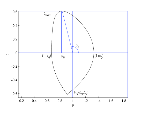
Figure 1: The boundary determined by the parametric Eqs. (20)-(23)

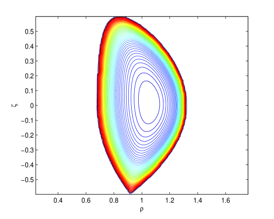
Figure 2: The equilibrium configuration in connection with the numerical solution of the GS-like equation [Eqs. (17)-(18)] for peaked toroidal current density $A=B=-1$ [Eq. (11)]. The magnetic surfaces are nearly the same for the respective equilibrium with hollow $J_{\phi}$ ($\tilde{A}=\tilde{B}=0$).

We adopt the numerical integration scheme described in detail in Sec. 4 of our previous paper kui1 using the nine point formula. Using the numerical algorithm associated with this formula for peaked toroidal current density ($A=B=-1$) we obtained the equilibrium shown in Fig. 2. The magnetic axis was found by the numerical procedure to be located at $(\rho_{a},\zeta_{a})=(1.0574,0.02)$. The numerical procedure converged to the actual solution of Fig. 2 after $N=2027$ iterations with a finite difference step size of $h=0.01$. We have taken $\alpha_{i}=0.0015$. At the boundary we have set $\Psi_{n}(b)=1.0$, while the numerical integration scheme turned out to give for the magnetic axis $\Psi_{n}(a)=0.0$. The configuration of Fig. 2 remains nearly unaffected when $J_{\phi}$ changes to hollow ($\tilde{A}=\tilde{B}=0$).

On the basis of the solution constructed we examined the characteristics for both equilibria with peaked and hollow $J_{\phi}$ by calculating the safety factor and certain equilibrium quantities as follows. For axisymmetric plasmas the safety factor can be put in the form

$$q(\Psi_{n})=\frac{1}{2\pi}\int_{0}^{2\pi}Q(\Psi_{n},\theta)d\theta$$ (24)

where

$$Q(\Psi_{n},\theta)=Q_{0}\frac{[(\rho-1)^{2}+\zeta^{2}]}{|(\rho-1)(\Psi_{n})_{,\rho}+\zeta(\Psi_{n})_{,\zeta}|}$$ (25)

and $Q_{0}\simeq 2.28$ is a dimensionless constant. The variation of the safety factor for peaked $J_{\phi}$ increasing monotonically from the magnetic axis to the plasma boundary is shown in Fig. 3. The profile of $J_{\phi}$ on the midplane $\zeta=0$ which vanishes on the boundary is shown in Fig. 4(above), while the respective hollow, current-hole like profile of $J_{\phi}$ is shown in Fig. 4(below). Since in the later case $J_{\phi}$ vanishes on axis the safety factor tends to infinity thereon and the equilibrium in the central region has negative magnetic shear. Current hole equilibria of this kind have been observed in JET hast and JT-60U fusu .

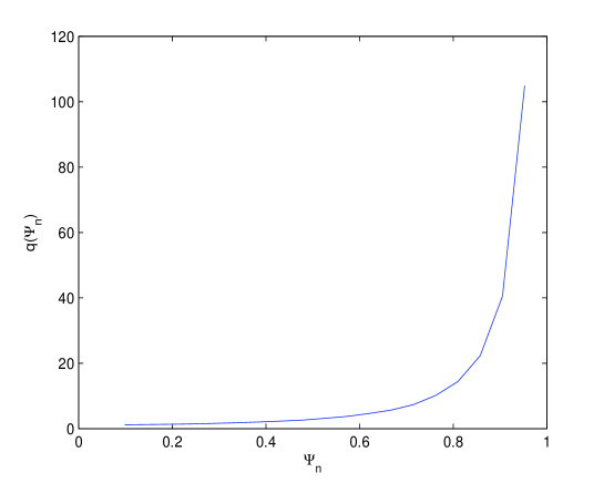
Figure 3: Variation of the safety factor for the equilibrium of Fig. 2 from the magnetic axis to the boundary for peaked on axis $J_{\phi}$. At the magnetic axis we have $q_{a}=1.17$.

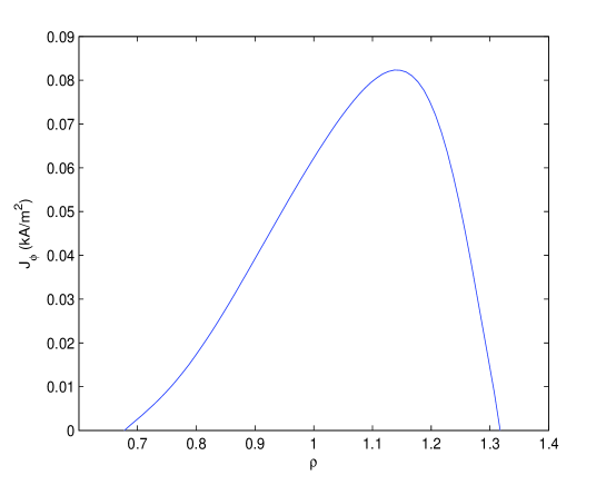
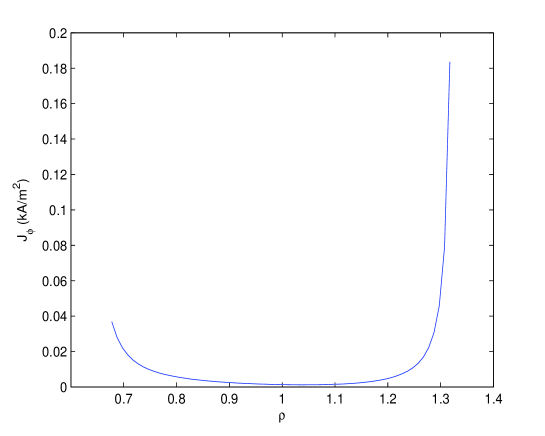
Figure 4: Peaked on axis toroidal current density for $A=B=-1$ in connection with the equilibrium of Fig. 2. (above) and respective hollow $J_{\phi}$ for $\tilde{A}=\tilde{B}=0$ (below).

The toroidal ion fluid velocity $U_{i\phi}$ is given by

$$U_{i\phi} = \frac{1}{n}\int\,v_{\phi}fd^{3}v$$ (26)

$$= \frac{\frac{V_{i\phi}\alpha_{i}(\rho/\rho_{n})\Psi_{n}}{[1-\beta(\rho^{2}/\rho_{n}^{2})]^{3/2}}exp\left(\frac{\Psi_{n}^{2}}{1-\beta(\rho^{2}/\rho_{n}^{2})}\right)}{1+\frac{\alpha_{i}}{\sqrt{1-\beta(\rho^{2}/\rho_{n}^{2})}}exp\left(\frac{\Psi_{n}^{2}}{1-\beta(\rho^{2}/\rho_{n}^{2})}\right)}$$

This for the two equilibria considered is plotted in Fig. 5. Note that the profile shapes are similar to the respective shapes of the current density profiles. Associated electric field profiles are given in Fig. 6.

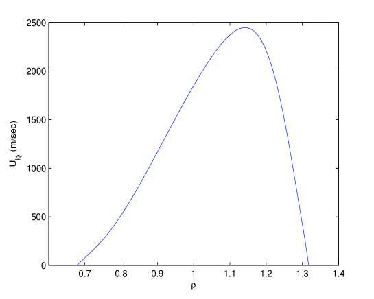
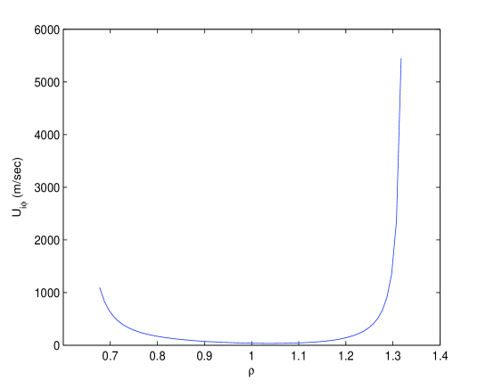
Figure 5: The ion fluid velocity profile on the midplane $z=0$ for the equilibrium with peaked $J_{\phi}$ (above) and hollow $J_{\phi}$ (below).

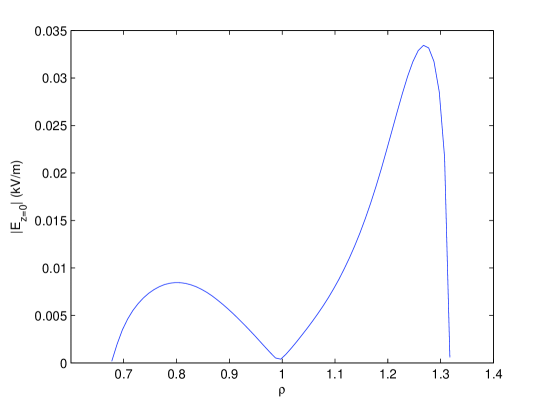
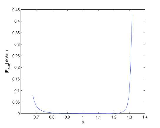
Figure 6: The electric field profile on the midplane $z=0$ for the equilibrium with peaked $J_{\phi}$ (above) and hollow $J_{\phi}$ (below).

According to frei (p. 14 therein) the total pressure tensor can be defined as

$$P_{kl} = P_{kl}^{i}+P_{kl}^{e}=$$

$$= M\int(v_{k}-U_{ik})(v_{l}-U_{il})d^{3}v+$$

$$+ m\int(v_{k}-U_{ek})(v_{l}-U_{el})d^{3}v,\;\;\;(k,l=r,\phi,z)$$

where $P_{kl}^{i}$, $P_{kl}^{e}$ are the pressure tensors of the ion and electron fluids and $U_{i\phi},\;U_{e\phi}$ are the ion and electron fluid velocities given by $U_{i\phi}=(1/n_{i})\int v_{\phi}f_{i}d^{3}v$ and $U_{e\phi}=(1/n_{e})\int v_{\phi}f_{e}d^{3}v$. In the limit of $V_{i\phi}\longrightarrow 0$ we recover the usual formula of $n_{0}k(T_{i}+T_{e})$ for the total pressure. For the distribution functions (II) the tensor becomes diagonal and anisotropic and we have $P_{rr}=P_{zz}:=P_{1}$ and $P_{\phi\phi}:=P_{2}$. Here

$$P_{1} := MI_{i}+mI_{e}=M\int v_{r}^{2}f_{i}d^{3}v+m\int v_{r}^{2}f_{e}d^{3}v$$

$$P_{2} = MJ_{i}+mJ_{e}=M\int(v_{\phi}-U_{i\phi})^{2}f_{i}d^{3}v+$$

$$+ m\int(v_{\phi}-U_{e\phi})^{2}f_{e}d^{3}v$$

Computing the integrals $I_{i},\;I_{e},\;J_{i},\;J_{e}$ we calcualted $P_{1}$, $P_{2}$ and the index of anisotropy

$$\omega:=\frac{|P_{2}-P_{1}|}{P_{1}}$$ (29)

The calculation though lengthy and tedious is straightforward. According to the results shown in Fig. 7, $P_{1}$ and $P_{2}$ decrease very weakly from the magnetic axis to the plasma boundary, irrespective of the shape of the current density profile.Similar is the behavior of the density variation given in Fig. 8 but the anisotropy index shown in Fig. 9 is different; the latter follows the respective variation of the current density profile. Apparently, such nearly flat pressure and density profiles are not representative for tokamaks. They just may be regarded as an approximation of the nearly flat pressure and density profiles observed during the L-H transition in the central region inside the edge pedestal at which the pressure drops sharply giving rise to the ELMs activity. This edge region can not be described by the equilibrium solutions constructed here; in particular, we had a difficulty to make $P_{1}$ and $P_{2}$ vanish on the boundary. This in addition to numerical reasons should be related with the fact that Vlasov theory involves particle orbits which, unlike fluid theories, are not compatible with a fixed boundary; in this sense Vlasov is not appropriate to describe fixed boundary equilibria in the region close to the boundary.

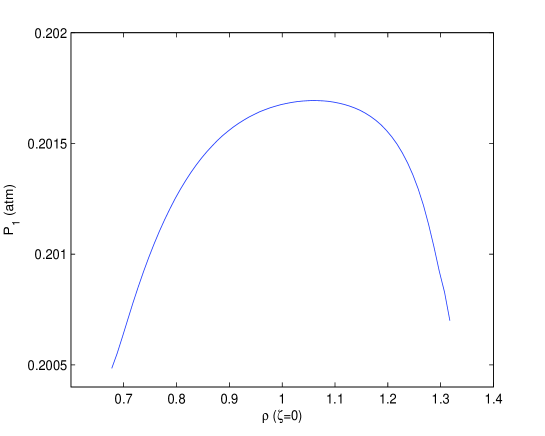
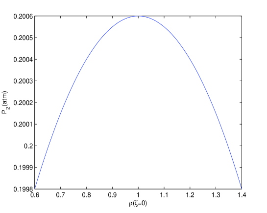
Figure 7: Profiles of the pressures $P_{1}$ and $P_{2}$ for the equilibrium with peaked $J_{\phi}$. Similar in shape are the respective pressure profiles with hollow $J_{\phi}$.

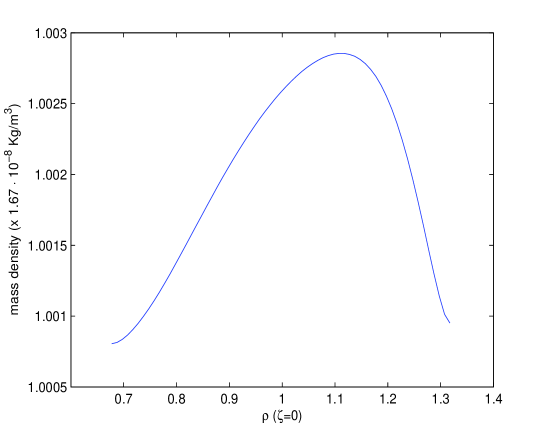
Figure 8: Density profile for the equilibrium with peaked $J_{\phi}$. Similar in shape is the density profile for the equilibrium with hollow $J_{\phi}$.

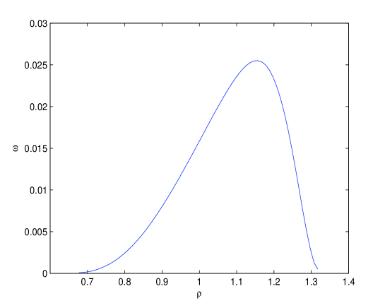
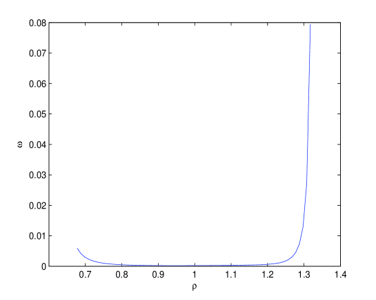
Figure 9: The pressure anisotropy index for the equilibrium with peaked $J_{\phi}$ (above) and hollow $J_{\phi}$ (below).

V Summary

In the framework of Maxwell-Vlasov theory we have derived a transcendental GS-like equation [Eqs. (17)-(18)] for quasineutral axisymmetric plasmas by selecting exponentially deformed Maxwellian ion and electron distribution functions depending on the two known constants of particle motion [Eqs. (10)]. Then we have solved this equation numerically for a tokamak pertinent fixed diverted plasma boundary. To avoid unphysical perpendicular drifts on axis the electric filed was provisioned to vanish thereon. Depending on the symmetry properties of the distribution functions in connection with the values of pertinent free parameters, we derived equlibria with toroidal current density profiles either peaked on axis or hollow. Both equilibria have nearly the same magnetic surfaces, sheared toroidal ion flow and diagonal anisotropic pressure tensor with different toroidal and poloidal elements. The profiles of the toroidal velocity and of the pressure isotropy index are similar to the respective profiles of the current density. However, the profiles of the pressure elements being nearly flat just may approximately represent respective experimental profiles in the central region developed during the L-H transition.

It is interesting to pursue obtaining other Vlasov equilibria with alternative choices of distribution functions, in particular distribution functions potentially creating more realistic pressure profiles. This may require numerical integrations in the velocity space which coupled with spatial integrations constitute a challenging problem. Also, since poloidal flows play a role in the transitions to improved confinement regimes in tokamaks it is desirable that these equilibria involve flows of arbitrary direction. However, as already mentioned in Sec. I, this remains a tough open problem requiring additional Vlasov constants of motion.

Aknowledgment

This work has been carried out within the framework of the EUROfusion Consortium and has received funding from (a) the National Programme for the Controlled Thermonuclear Fusion, Hellenic Republic, (b) Euratom research and training programme 2014-2018 under grant agreement No 633053. The views and opinions expressed herein do not necessarily reflect those of the European Commission.

References

- (1) P. J. Channell, Phys. Fluids 19, 1541 (1976).
- (2) S. M. Mahajan, Phys. Fluids B 1, 43 (1989).
- (3) N. Attico, F. Pegoraro, Phys. Plasmas 6, 767 (1999).
- (4) F. Mottez, Phys. Plasmas 10, 2501 (2003).
- (5) C. Montagna, F. Pegoraro, Phys. Plasmas 14, 042103 (2007).
- (6) C. R. Stark, T. Neukirch, Phys. Plasmas 19, 012115 (2012).
- (7) G. Belmont, N. Aunai, R. Smets, Phys. Plasmas 19 022108 (2012).
- (8) S. A. Lazerson, J. Plasma Phys. 77 31 (2011).
- (9) H. E. Mynick, W. M. Sharp, A. N. Kaufman, Phys, Fluids 22 1478 (1979).
- (10) K. Schindler, Physics of space plasma activity (Cambridge University Press, 2007)
- (11) G. N. Throumoulopoulos, H. Tasso, Analytic, quasineutral, two-dimensional Maxwell-Vlasov equilibria, arXiv:0909.1745v2 (2009).
- (12) H. Tasso, G. N. Throumoulopoulos, J. Phys. A 40, F631 (2007).
- (13) H. Tasso, G. N. Throumoulopoulos, Eur. Phys. J. D 68, 175 (2014).
- (14) J. P. Freidberg, in Ideal Magnetohydrodynamics (Plenum Press, 1987), pp. 14, 108.
- (15) Ap Kuiroukidis and G. N. Throumoulopoulos, J. Plasma Phys. 80, 27 (2014).
- (16) N. C. Hawkes, B. C. Stratton, T. Tala et al., Phys. Rev. Lett. 87, 115001 (2001).
- (17) T. Fujita T. Suzuki, T. Oikawa et al., Phys. Rev. Lett. 95, 075001 (2005).