Piecewise smooth systems near a
co-dimension 2 discontinuity manifold:
can one say what should happen?

Abstract.

We consider a piecewise smooth system in the neighborhood of a co-dimension 2 discontinuity manifold $\Sigma$ (intersection of two co-dimension 1 manifolds). Within the class of Filippov solutions, if $\Sigma$ is attractive, one should expect solution trajectories to slide on $\Sigma$. It is well known, however, that the classical Filippov convexification methodology does not render a uniquely defined sliding vector field on $\Sigma$. The situation is further complicated by the possibility that, regardless of how sliding on $\Sigma$ is taking place, during sliding motion a trajectory encounters so-called generic first order exit points, where $\Sigma$ ceases to be attractive.

In this work, we attempt to understand what behavior one should expect of a solution trajectory near $\Sigma$ when $\Sigma$ is attractive, what to expect when $\Sigma$ ceases to be attractive (at least, at generic exit points), and finally we also contrast and compare the behavior of some regularizations proposed in the literature, whereby the original piecewise smooth system is replaced –in a neighborhood of $\Sigma$– by a smooth differential system.

Through analysis and experiments in $\mathbb{R}^{3}$ and $\mathbb{R}^{4}$, we will confirm some known facts, and provide some important insight: (i) when $\Sigma$ is attractive, a solution trajectory indeed does remain near $\Sigma$, viz. sliding on $\Sigma$ is an appropriate idealization (of course, in general, one cannot predict which sliding vector field should be selected); (ii) when $\Sigma$ loses attractivity (at first order exit conditions), a typical solution trajectory leaves a neighborhood of $\Sigma$; (iii) there is no obvious way to regularize the system so that the regularized trajectory will remain near $\Sigma$ as long as $\Sigma$ is attractive, and so that it will be leaving (a neighborhood of) $\Sigma$ when $\Sigma$ looses attractivity.

We reach the above conclusions by considering exclusively the given piecewise smooth system, without superimposing any assumption on what kind of dynamics near $\Sigma$ (or sliding motion on $\Sigma$) should have been taking place. The only datum for us is the original piecewise smooth system, and the dynamics inherited by it.

1. Introduction

Consider the following piecewise smooth (PWS) system:

(1.1) $$\dot{x}=f(x)\ ,\,\ f(x)=f_{i}(x)\ ,\,\ x\in R_{i}\ ,\,i=1,2,3,4,$$

for $t\in[0,T]$, and where, for $i=1,2,3,4$, $R_{i}\subseteq\mathbb{R}^{n}$ are open, disjoint and connected sets, and $\mathbb{R}^{n}=\overline{\bigcup_{i}R_{i}}$. System (1.1) is subject to initial condition $x(0)=x_{0}$, prescribed in one of the regions $R_{i}$’s. In (1.1), for any $i=1,2,3,4$, each $f_{i}$ is smooth in $R_{i}$, so that there is a classical solution in each region $R_{i}$, but the solution is not properly defined on the boundaries of these regions. We assume that these regions are separated (locally) by an implicitely defined smooth manifold $\Sigma$ of co-dimension $2$. That is, we have

(1.2) $$\Sigma=\{x\in\mathbb{R}^{n}\ :\,h(x)=0\,,\quad h:\ \mathbb{R}^{n}\to\mathbb{R}^{2}\}\,,$$

and for all $x\in\Sigma$: $h(x)=\begin{bmatrix}h_{1}(x)\\ h_{2}(x)\end{bmatrix}$, $\nabla h_{j}(x)\neq 0$, $h_{j}\in{\mathcal{C}}^{k},\ k\geq 2$, $j=1,2$, and $\nabla h_{1}(x),\nabla h_{2}(x)$, are linearly independent on (and in a neighborhood of) $\Sigma$. It is useful to think of $\Sigma=\Sigma_{1}\cap\Sigma_{2}$, where $\Sigma_{1}=\{\ x:\ h_{1}(x)=0\}$, and $\Sigma_{2}=\{\ x:\ h_{2}(x)=0\}$, are co-dimension 1 manifolds. Finally, without loss of generality we will henceforth use the following labeling of the four regions $R_{i}$, $i=1,2,3,4$:

(1.3) $$\begin{split}&R_{1}:\quad\text{when}\quad h_{1}<0\ ,\,h_{2}<0\ ,\qquad R_{2}:\quad\text{when}\quad h_{1}<0\ ,\,h_{2}>0\ ,\\ &R_{3}:\quad\text{when}\quad h_{1}>0\ ,\,h_{2}<0\ ,\qquad R_{4}:\quad\text{when}\quad h_{1}>0\ ,\,h_{2}>0\ .\end{split}$$

For later use, we will also adopt the notation $\Sigma_{1,2}^{\pm}$ to denote the set of points $x\in\Sigma_{1}$ or $\Sigma_{2}$, for which we also have $h_{2}(x)\gtrless 0$ or $h_{1}(x)\gtrless 0$. E.g., $\Sigma_{1}^{+}=\{x\in\Sigma_{1}\,\,\ \text{and}\,\,\ h_{2}(x)>0\}$. Finally, we will denote with

(1.4) $$w^{i}_{j}(x)=\nabla h_{i}(x)^{\top}f_{j}(x)\ ,\,\,i=1,2,\ j=1,2,3,4\ ,$$

the projections of the vector fields in the normal directions to the manifolds.

For (1.1), a classical solution in general cannot exist on the boundaries of the given regions, and several concepts of generalized solution have been proposed during the years (see [4] for a beautiful exposition on different solutions concepts). We will restrict attention to Filippov solutions, [15], consisting of absolutely continuous functions whose derivative is in the convex hull of the neighboring vector fields almost everywhere.

1.1. Co-dimension 1

In the case of one single discontinuity manifold of co-dimension 1, Filippov methodology has provided a widely accepted mathematical framework to understand motion on the discontinuity surface.

Consider a discontinuity manifold $\Sigma=\{x\in\mathbb{R}^{n}:\ h(x)=0\ ,\,\ h:\mathbb{R}^{n}\to\mathbb{R}\ \}$, separating two regions $R_{1}$ (where $h(x)<0$) and $R_{2}$ (where $h(x)>0$), with respective vector fields $f_{1}$ and $f_{2}$. Assuming that $\Sigma$ is attractive, a condition that is satisfied when

$$\nabla h^{T}f_{1}>0\quad\text{and}\quad\nabla h^{T}f_{2}<0\ ,\,\ x\in\Sigma\ ,$$

then sliding motion on $\Sigma$ takes place with vector field

(1.5) $$f_{\text{F}}:=(1-\alpha)f_{1}+\alpha f_{2}\ ,\qquad\alpha=\frac{\nabla h^{T}f_{1}}{\nabla h^{T}(f_{1}-f_{2})}\ .$$

Filippov theory provides also first order exit conditions: if one of $f_{1}$ or $f_{2}$ (but not both) become tangent to $\Sigma$, then $\alpha=0$ or $1$, $\Sigma$ loses attractivity, and the solution trajectory generically will leave $\Sigma$ tangentially (and smoothly) to enter in $R_{1}$ with vector field $f_{1}$, or in $R_{2}$ with vector field $f_{2}$. Furthermore, it has been understood for a long time that the limiting behavior of the iterates obtained with Euler method near $\Sigma$ leads to the selection of the Filippov sliding vector field itself (e.g., see [26], Chapter 3, Section 1.1) whenever $\Sigma$ is attractive, and that the Euler iterates leave a neighborhood of $\Sigma$ when $\Sigma$ loses attractivity.

1.2. Co-dimension 2

However, when $\Sigma$ is of the form (1.2), an obvious lack of uniqueness (in general) arises in the construction of a Filippov vector field sliding on $\Sigma$. In fact, on $\Sigma$, Filippov methodology now leads to the requirement that the vector field satisfies the following (for positive values of $\lambda_{1},\dots,\lambda_{4}$):

(1.6) $$\begin{split}f_{\text{F}}&:=\lambda_{1}f_{1}+\lambda_{2}f_{2}+\lambda_{3}f_{3}+\lambda_{4}f_{4}\ ,\quad\text{where}\\ &\begin{bmatrix}w^{1}_{1}&w^{1}_{2}&w^{1}_{3}&w^{1}_{4}\\ w^{2}_{1}&w^{2}_{2}&w^{2}_{3}&w^{2}_{4}\\ 1&1&1&1\end{bmatrix}\begin{bmatrix}\lambda_{1}\\ \lambda_{2}\\ \lambda_{3}\\ \lambda_{4}\end{bmatrix}=\begin{bmatrix}0\\ 0\\ 1\end{bmatrix}\ ,\end{split}$$

which is clearly an underdetermined system of equations. Indeed, even when $\Sigma$ is attractive, in general (1.6) has a one parameter family of solutions and hence of possible Filippov sliding vector fields.

Remarks 1.1.

 

• Characterization of attractivity of $\Sigma$ in the present co-dimension 2 case is considerably more elaborate than in the case of co-dimension 1. We will assume that $\Sigma$ is either attractive by subsliding (see [10] ) or attractive by spiralling (see [7]), in the form recalled below in Definition 1.2.

• In the present case, the general lack of uniqueness is not resolved by considering the limiting behavior of the Euler iterates near $\Sigma$. In fact, as already noted in [15], the limit of the Euler iterates selects one specific element of the one-parameter family of Filippov solutions.

Definition 1.2.

$\Sigma$ (or a portion of it) is attractive upon sliding if it is reached in finite time by solution trajectories for any given nearby initial condition, and further there is sliding motion towards $\Sigma$ along at least one of the $\Sigma_{1,2}^{+}$. When there is sliding motion towards $\Sigma$ along all of the $\Sigma_{1,2}^{\pm}$’s then we say that $\Sigma$ is nodally attractive. $\Sigma$ (or portion of it) is attractive by spiralling if $\Sigma$ is reached in finite time by trajectories for any given nearby initial condition, and there is clockwise or counter clockwise motion around $\Sigma$ (and no sliding on $\Sigma_{1,2}^{\pm}$) for the functions $h_{1}(x)$ and $h_{2}(x)$.

When $\Sigma$ is attractive, in the literature there have been at least two systematic proposals to select the coefficients $\lambda_{i}$’s in (1.6), leading to sliding vector fields of Flilippov type on $\Sigma$: the bilinear and the moments vector fields. The former has been extensively studied, see [1, 2, 10, 17] for example, and it consists in choosing the sliding vector field in the form

(1.7) $$\begin{split}f_{B}&:=(1-\alpha)[(1-\beta)f_{1}+\beta f_{2}]+\alpha[(1-\beta)f_{3}+\beta f_{4}]\ ,\\ (\alpha,\beta):&\,\begin{bmatrix}w^{1}_{1}&w^{1}_{2}&w^{1}_{3}&w^{1}_{4}\\ w^{2}_{1}&w^{2}_{2}&w^{2}_{3}&w^{2}_{4}\end{bmatrix}\begin{bmatrix}(1-\alpha)(1-\beta)\\ (1-\alpha)\beta\\ \alpha(1-\beta)\\ \alpha\beta\end{bmatrix}=\begin{bmatrix}0\\ 0\end{bmatrix}\ .\end{split}$$

The moments method has been recently introduced in [9] and consists in solving the linear system in (1.6), by appending to it the extra relation

(1.8) $$\begin{bmatrix}d_{1}&-d_{2}&-d_{3}&d_{4}\end{bmatrix}\begin{bmatrix}\lambda_{1}\\ \lambda_{2}\\ \lambda_{3}\\ \lambda_{4}\end{bmatrix}=0\ ,\quad d_{i}=\|w_{i}\|_{2}\ ,\,\ i=1,2,3,4\ .$$

The two choices above generally lead to distinct solution trajectories, a chief difference between them being the behavior of the bilinear and moments trajectories at so-called generic tangential exit points. These were introduced in [10], and are values of $x\in\Sigma$, where one (and just one) of the sliding vector fields on $\Sigma_{1}^{\pm}$ or $\Sigma_{2}^{\pm}$ is itself tangent to $\Sigma$ (exit vector field). The moments vector field automatically aligns with the exit vector field, whereas the bilinear vector field does not.

An important question, and one which we will try to answer in this work is: what should happen to trajectories of (1.1) in a neighborhood of $\Sigma$, when $\Sigma$ loses attractivity (according to generic first order exit conditions)?

1.3. Regularize

If natura non facit saltum, then (1.1) is either a description of an innatural system or a wrong model. Probably, whenever it is set forth, it is neither innatural nor wrong, though it may be a little of both things, perhaps because the model should be complemented by some missing information (the 20 years old exposition of Seidman in [23] is still worthwhile reading). Regardless, the above 18th century motto suggests considering a regularized version of (1.1), by replacing it with a smooth differential system. Of course, we must assume that we do not have knowledge of where (1.1) comes from, if from anywhere at all, otherwise we should surely use this knowledge. However, in the absence of further insight, it is not obvious how one should globally regularize the system, and several possibilities for globally regularizing the system have been proposed in the literature.

Arguably, the most studied regularization techniques are what we may call the “singular perturbation” and “sigmoid blending” techniques. The paper [24] was the first seminal work on the singular perturbation approach, followed by the more recent works [18], as well as [13], [16], [17] and, in the context of gene regulatory networks, [20]. The first systematic exposition of blending was the beautiful work [1]. But, in the end, these techniques are all rather similar and amount to a regularization of the bilinear vector field. This can be done locally, just in a neighborhood of $\Sigma$, say using a cutoff function (as we do in Section 2), or more globally, perhaps through use of hyperbolic $\arctan$ functions to connect different vector fields.

In this work, we are exclusively concerned with local regularizations, hence those that alter the given problem only in a neighborhood of $\Sigma$. In this case, the above mentioned regularization proposals share some common traits, the most important ones being that, outside of a neighborhood of $\Sigma$, the regularized vector field effectively reduces to the original vector fields, and that the regularization depends on a small parameter (or several small parameters) in such a way that as the parameter(s) go to $0$, the neigborhood collapses onto $\Sigma$. The first fact is surely a reasonable property, since, away from $\Sigma$, there is a well defined smooth vector field depending on where the trajectory is, be it one of the original $f_{1,2,3,4}$ or one of the Filippov sliding vector fields on the surfaces $\Sigma_{1,2}$. The second fact may be a bit more controversial, since the regularized trajectory will typically select a specific sliding motion on $\Sigma$ (when $\Sigma$ is attractive), as the neighborhood collapses onto $\Sigma$; however, as it is well understood, and as we will also see, different regularizations do behave differently. As noted by Utkin ( [26] ), given that in a neighborhood of $\Sigma$ there are non-unique dynamics, the inherited dynamics on $\Sigma$ (sliding motion) does depend on the choice of regularization. But, this being the case, is there an appropriate way to evaluate different regularizations? To answer this question, we must first decide how we should evaluate dynamics.

1.4. Evaluate dynamics

The first observation is that when we evaluate the dynamics of (1.1) we should distinguish between the two cases (i) and (ii) below.

• The PWS smooth system (1.1) is just a “convenient” formalism: there is a “true” smooth system, defined globally, but it is simpler to replace it by a PWS one. For example, this is the case for problems arising in gene regulatory networks ([19], [5]). In these cases, one knows what is the desired behavior in a neighborhood of $\Sigma$: it is the behavior of the original problem! However, one must be careful in replacing the true system by (1.1), since it is not clear that the dynamics of the purely PWS system reflect the dynamics of the original problem; this was already noted in works such as [21] and [23] relative to a discontinuity surface of co-dimension 1. But, doesn’t this discrepancy mean that representing the original problem as a PWS one was not an appropriate modeling simplification in the first place?

• The problem arises as piecewise smooth problem, or we do not have sufficient knowledge of an underlying “true” problem (if any); for example, in bang-bang control, or in dry friction models. In our opinion, in these cases when there is no (knowledge of an) underlying “true” dynamics that one is trying to recover, the choices we make must be consistent with the PWS formulation. This is the case in which we are interested.

The above consideration (ii) leads us to restrict to the model (1.1) as the system we are given and it is this system that we will study. This realization motivates us (and it has motivated us for several years) to look at the global properties of the discontinuity surface, and to decide on what is appropriate based on whether or not the surface attracts the dynamics of the PWS system for initial conditions off the discontinuity surface itself. In our opinion, it is not easy to justify studying (1.1) by assuming a specific form of an underlying system from where (1.1) arises as some form of limiting process. In other words, whereas it is surely legitimate (and by no means trivial) to study the limiting behavior of a specific choice of regularized vector field defined in a neighborhood of $\Sigma$, this may actually have a restricted scope of applicability compared to (1.1). As already noted by Utkin (see [25, p.44]), once one has replaced (1.1) with a smoothed version of it, the stability of sliding motion on $\Sigma$ is inherited by that of the dynamics of the regularized field. But, is this consistent with the formulation (1.1)?

For the given PWS system (1.1), we believe that it is its dynamics near the discontinuity manifold that determines the appropriate behavior of a trajectory. This dynamics is what we will try to capture in this work. Moreover, our main interest is in the case when the discontinuity manifold transitions from being attractive to not attractive for the trajectories of the original discontinuous system: in this case, will (or should) a trajectory (even an ideal trajectory, sliding on the manifold) feel this loss of attractivity, and hence leave a neighborhood of $\Sigma$?

Therefore, without assuming any form of idealized motion on $\Sigma$, we can reformulate our main task as follows:

“how should we evaluate the dynamics of (1.1) in a neighborhood of $\Sigma$?”

In principle, one may want to do this by studying the dynamics of a regularized problem, and we have already mentioned some possibilities, such as sigmoid blending and singular perturbation techniques. E.g., see [1, 13, 16, 17, 18, 24]. We emphasize once more that these choices (as noted by Alexander and Seidman for blending, and by Teixeira et alia. for singular parturbation) remove the ambiguity of how sliding on $\Sigma$ occurs, but these choices are effectively modeling assumptions, and we should ask if they render a behavior of the dynamics on $\Sigma$ that is consistent with that of (1.1).

Other possibilities have also been set forth in the literature, see [1] for further references.

• Euler broken line approximation. This is simple to do, and it consists in replacing (1.1) by a Euler method approximation with constant stepsize, call it $\tau$. We have experimented extensively with this technique, see below. [The eventuality, of probability 0, that an Euler iterate lands exactly on a discontinuity surface can be handled in different ways; e.g., by randomly selecting one of the neighboring vector fields, or by retaining the last vector field used.]

• Hysteresis (or delay) approximation. This approach appears in [26] for a surface of co-dimension 1. For the case of $\Sigma$ of co-dimension 2, it has been studied first in [2] and then in [8], always in the case of nodally attractive $\Sigma$. The idea here is that one has a region $U_{\epsilon}$ around $\Sigma$ (called a chatterbox in [2]), and uses the same vector field, say $f_{1}$, not only in the region $R_{1}$, but until the boundary of $U_{\epsilon}$ in a different region is reached; at that point, a switch to the appropriate vector field in the new region is performed. The rationale for this approach is that one does not notice immediately that a discontinuity surface is reached, but there is a “delay” in appreciating this fact.

• Replacing (1.1) with a stochastic DE of Ito type: $\dot{x}=f_{i}(x)dt+\epsilon dw_{t}$. Again we note that there is zero probability of landing exactly on the discontinuity surface(s). The interesting feature of this approach is that it is bound to sample different vector fields around $\Sigma$. The disadvantage is that it makes quantitative predictions possible only in a statistical sense.

With the exception of (c), the other choices above effectively replace the original PWS with another deterministic dynamical system, possibly discrete (as in the case of Euler method). But, unfortunately, these new systems have their own dynamics, and it is unclear whether or not these are consistent with that of (1.1). See Section 4 for ample illustration of this fact. At the same time, each of the cases above has some distinguished features, that we will attempt to retain.

1.5. Proposal and Plan

Our proposal to evaluate the dynamics of (1.1) in a neighborhood of $\Sigma$ is to:

“consider the Euler iterates with random steps,”

with steps uniformly distributed about a reference stepsize. In other words, we want to retain the simplicity of looking at Euler iterates, but aim at retaining a certain amount of randomness in the process to avoid getting trapped by the purely Euler dynamics. Furthermore, in this work we will restrict to well-scaled vector fields $f_{i}$, $i=1,\dots,4$, with none of the $w^{i}_{j}$’s in (1.4) exceeding $1$ in absolute value. The reason for this is to avoid the numerical trajectory going too far away from $\Sigma$, and at the same time to attempt retaining the flavor of a hysteretical trajectory.

We will complement our experiments made with the above strategy, by also using other approaches. For example, Euler method with constant stepsizes, singular perturbation regularizations, and also numerical integration of (1.1) performed with variable stepsize integrators.

We emphasize that our goal is to reach some conclusions insofar as what should happen to a solution trajectory of (1.1) in a (small) neighborhood of $\Sigma$. We are not comparing methods, or different recipes of ideal sliding motion, but simply trying to evaluate the dynamics of (1.1) in the most plausible and honest way we can think of, without superimposing on (1.1) any extra modeling assumption.

Finally, one more caveat. Our examples are all of systems in $\mathbb{R}^{3}$ and $\mathbb{R}^{4}$, and the discontinuity surfaces $\Sigma_{1}$ and $\Sigma_{2}$ are planes; this makes it easier to visualize and understand things. Higher dimensional state space, and non-planar discontinuity surfaces, can surely bring new phenomena into play, but we have no reason to suspect that the basic picture that emerges in our study, with the dichotomy between attractivity and lack of attractivity of $\Sigma$, will be modified substantially.

The remainder of this work is structured as follows. In Section 2, we consider a prototypical regularization of the bilinear vector field (1.7), and give sufficient (and sharp) conditions guaranteeing that the regularized solution converges to a sliding solution on $\Sigma$ according to (1.7). In Section 3, we give some details of how we implemented the above mentioned proposal, particularly of what practical criteria we adopted to detect “exiting” from a neighborhood of $\Sigma$. In Section 4, we illustrate through several examples the different things that can happen, and their dependence on the adopted simulation choice.

2. Bilinear interpolant regularization: solutions behavior and fast slow dynamics

Space regularizations are often employed in literature as an analytical mean to model the switching mechanism of a discontinuous system, see [2, 13, 16, 17, 18, 24, 25]. Typically, these regularizations are one parameter families of vector fields with different time scales in a neighborhood of the sliding surface $\Sigma$, namely a slow dynamics tangent to $\Sigma$ and a fast one normal to $\Sigma$. In what follows, we consider regularizations for Filippov discontinuous systems as in (1.1), but other approaches are available in the literature for non-smooth systems that are not of Filippov’s type, for example control systems with nonlinear control, as in [25, 26]. When the regularization parameter goes to zero, the regularized solution converges to a solution of Filippov’s differential inclusion ([15, Theorem 1, §8]). It follows that, if $\Sigma$ is a codimension $1$ discontinuity surface, for any regularization that satisfies the assumptions of [15, Theorem $1$, $\S 8$], the corresponding solution will converge to the unique sliding Filippov solution on $\Sigma$ as the regularization parameter goes to zero. But if $\Sigma$ has codimension $k\geq 2$, then the ambiguity of Filippov’s selection will reflect also in the amibiguity of the limit of regularized solutions (in other words, the limit will depend on the chosen regularization).

Our goal in this section is to study the limiting behavior of the solutions of a certain regularization, namely the bilinear interpolant, or simply bilinear, regularization (2.2) below. This regularization (or a close relative) has often been employed and studied in the literature; see [1, 2, 22, 23, 13, 17, 16, 18]. More specifically, we will study when the solution of the bilinear regularization converges to the solution of a particular selection of the Filippov’s vector field: the sliding bilinear vector field (1.7). When $\Sigma$ is nodally attractive, this convergence has been shown in [1, Theorem 5.1], and -under the same assumption- in [13] it is shown that the bilinear regularized vector field converges to the bilinear sliding vector field. In what follows, we relax the hypothesis on attractivity of $\Sigma$, and simply assume that $\Sigma$ is attractive in finite time, i.e. all trajectories with initial conditions in a neighborhood of $\Sigma$ will reach $\Sigma$ in finite time. This can be achieved either upon sliding along $\Sigma_{1}$ and/or $\Sigma_{2}$ ($\Sigma$ is attractive upon sliding), or spiralling around $\Sigma$ ($\Sigma$ is spirally attractive); see Definition 1.2. For later reference, and under the stated attractivity assumptions of $\Sigma$, we note that the algebraic system (1.7) has a unique solution $(\alpha,\beta)$ in $(0,1)^{2}$.

For simplicity, we assume that $\Sigma$ is the intersection of the hyperplanes $\Sigma_{1}=\{x\in\mathbb{R}^{n}|x_{1}=0\}$ and $\Sigma_{2}=\{x\in\mathbb{R}^{n}|x_{2}=0\}$. Then, we consider the $\epsilon$-neighborhood $S$ of $\Sigma$: $S=\{x_{1},x_{2}:\ -\epsilon\leq x_{1},x_{2}\leq\epsilon\}$, and two smooth (at least $C^{1}$) monotone functions (the functions of course depend on $\epsilon$, but for notational simplicity this dependence on $\epsilon$ is omitted) $\alpha,\beta\ :\ \mathbb{R}\to[-1,1]$ interpolating at $\pm\epsilon$, as follows:

(2.1) $$\alpha(\epsilon)=\beta(\epsilon)=1,\,\ \alpha(-\epsilon)=\beta(-\epsilon)=0,\,\ \alpha^{\prime}(x_{1}),\beta^{\prime}(x_{2})>0,\text{ for }-\epsilon<x_{1},x_{2}<\epsilon\ .$$

We call bilinear regularization the following one parameter family of vector fields

(2.2) $$\begin{split}f_{\mathcal{B}}^{\epsilon}(x)=(1-\alpha(x_{1}))\left[(1-\beta(x_{2}))f_{1}(x)+\beta(x_{2})f_{2}(x)\right]+\\ \alpha(x_{1})(\left[(1-\beta(x_{2}))f_{3}(x)+\beta(x_{2})f_{4}(x)\right]\ .\end{split}$$

To be specific, in what follows, we have taken

(2.3) $$\alpha(x_{1})=\left\{\begin{matrix}1&x_{1}>\epsilon\\ \frac{1}{2}+\frac{x_{1}}{4\epsilon}(3-(\frac{x_{1}}{\epsilon})^{2})&x_{1}\in[-\epsilon,\epsilon]\\ 0&x_{1}<-\epsilon\end{matrix}\right.,\,\ \beta(x_{2})=\left\{\begin{matrix}1&x_{2}>\epsilon\\ \frac{1}{2}+\frac{x_{2}}{4\epsilon}(3-(\frac{x_{2}}{\epsilon})^{2})&x_{2}\in[-\epsilon,\epsilon],\\ 0&x_{2}<-\epsilon\end{matrix}\right.$$

but other choices of a $C^{1}$ monotone interpolant could be considered. Clearly, a choice of two different parameters for $\alpha$ and $\beta$, respectively $\epsilon_{\alpha}$ and $\epsilon_{\beta}$, could also be considered (e.g., see [22]), and this would be justified if, for example, it is known a priori that the trajectories of un underlying physical system approach the two surfaces $\Sigma_{1}$ and $\Sigma_{2}$ at different rates. Naturally, the choice of different parameters might lead to different qualitative behavior of the corresponding solutions, as we will see in Section 4.

Remark 2.1.

Often (e.g., see [1, 13, 18]), a simpler $C^{0}$ regularization is adopted, namely $\alpha(x_{1})=\frac{x_{1}+\epsilon}{2\epsilon}$, and similarly for $\beta(x_{2})$, possibly with different $\epsilon_{\alpha}$ and $\epsilon_{\beta}$. Proposition 2.6 is not meaningful in this case, whereas Proposition 2.7 holds with essentially the same proof. See also Remark 2.4.

Our goal is to study the behavior of solutions of $\dot{x}=f^{\epsilon}_{\mathcal{B}}(x)$ for $x\in S$, and to see when, for $\epsilon\to 0$, they converge to the sliding solution on $\Sigma$ with vector field $f_{B}$ as given in (1.7). In order to do so, we split $\dot{x}=f^{\epsilon}_{\mathcal{B}}(x)$ into fast and slow motions. For $(x_{1},x_{2})$ in $S$, we can rewrite (2.2) with respect to the variables $(\alpha,\beta,x_{3},\ldots,x_{n})$. For the sake of more compact notation, we let $y=(x_{3},\ldots,x_{n})$ and further $\dot{y}=g(\alpha,\beta,y)$. In these variables, the full system rewrites as

(2.4) $$\begin{split}\dot{\alpha}&=\frac{d\alpha}{dx_{1}}e_{1}^{T}f^{\epsilon}_{\mathcal{B}}(\alpha,\beta,y):=\frac{d\alpha}{dx_{1}}g_{1}(\alpha,\beta,y)\\ \dot{\beta}&=\frac{d\beta}{dx_{2}}e_{2}^{T}f^{\epsilon}_{\mathcal{B}}(\alpha,\beta,y):=\frac{d\beta}{dx_{2}}g_{2}(\alpha,\beta,y),\\ \dot{y}&=g(\alpha,\beta,y)\qquad\quad\end{split}$$

where $e_{i}$ is the standard $i$-th unit vector in $\mathbb{R}^{n}$, $i=1,2$. Notice that $\frac{d\alpha}{dx_{1}}$ and $\frac{d\beta}{dx_{2}}$ depend on $\epsilon$ and are strictly positive (inside $S$); from (2.3), they are equal to $\frac{3}{4\epsilon}(1-\frac{x_{i}^{2}}{\epsilon^{2}})$, with $i=1,2$. We refer to $\alpha$ and $\beta$ as the fast variables and to $y$ as the slow variable. We denote the solution of (2.4) as $(\alpha_{\epsilon}(\cdot),\beta_{\epsilon}(\cdot),y_{\epsilon}(\cdot))$.

Now, using (2.3), in (2.4), because of monotonicity of $\alpha$ and $\beta$, we can rewrite $x_{1}$ as a function of $\alpha$ and $x_{2}$ as a function of $\beta$. From (2.3), let $z=\frac{x_{1}}{\epsilon}$ and rewrite the first of (2.3), for $x_{1}\in[-\epsilon,\epsilon]$, as: $z^{3}-3z+4\alpha-2=0$. Using Vieta’s substitution $z=w+\frac{1}{w}$, we get the equation $w^{6}+(4\alpha-2)w^{3}+1=0$. Then $w^{3}=(1-2\alpha)\pm 2i\sqrt{\alpha-\alpha^{2}}$ and its third roots have modulus one, so that $z=w+\frac{1}{w}=\bar{w}+\frac{1}{\bar{w}}$ is real. Let $\varphi(\alpha)=Arg\left((1-2\alpha)+2i\sqrt{\alpha-\alpha^{2}}\right)$, then for $\alpha$ in [0,1], $\varphi(\alpha)$ is in $[0,\pi]$, and for $w(\alpha)=e^{i(\frac{\varphi(\alpha)}{3}+\frac{4}{3}\pi})$, the corresponding $z(\alpha)$ can be rewritten as $z(\alpha)=2\cos(\frac{\varphi(\alpha)}{3}+\frac{4}{3}\pi)$ and satisfies $z(0)=-1$ and $z(1)=1$, this $z(\alpha)$ is the function we are looking for. Same reasoning applies for $\beta$. Then system (2.4) rewrites as

(2.5) $$\begin{split}\epsilon\dot{\alpha}&=\frac{3}{4}\left(1-4\cos^{2}\left(\frac{\varphi(\alpha)}{3}+\frac{4}{3}\pi\right)\right)e_{1}^{T}f_{\mathcal{B}}(\alpha,\beta,y)\\ \epsilon\dot{\beta}&=\frac{3}{4}\left(1-4\cos^{2}\left(\frac{\varphi(\beta)}{3}+\frac{4}{3}\pi\right)\right)e_{2}^{T}f_{\mathcal{B}}(\alpha,\beta,y),\\ \dot{y}&=g(\alpha,\beta,y)\end{split}$$

with $\varphi(\gamma)=Arg\left((1-2\gamma)+2i\sqrt{\gamma-\gamma^{2}}\right)$. Notice that the function $\left(1-4\cos^{2}\left(\frac{\varphi(\gamma)}{3}+\frac{4}{3}\pi\right)\right)$ is strictly positive for $\gamma\in(0,1)$ and it is $0$ at $\gamma=0,1$. Following standard approaches for singularly perturbed systems, we set $\epsilon=0$ in (2.5) and obtain the following system

(2.6) $$\begin{split}0&=g_{1}(\alpha,\beta,y)\\ 0&=g_{2}(\alpha,\beta,y)\\ \dot{y}&=g(\alpha,\beta,y)\end{split}$$

Notice that solutions of (2.6) are sliding solutions on $\Sigma$ with bilinear vector field $f_{B}$ as in (1.7). Let $(\alpha^{*}(y),\beta^{*}(y))$ denote the solution of

(2.7) $$\begin{cases}g_{1}(\alpha^{*}(y),\beta^{*}(y),y)&=0\\ g_{2}(\alpha^{*}(y),\beta^{*}(y),y))&=0\end{cases}.$$

(Recall that, under the assumptions of attractivity by sliding or by spiralling, $(\alpha^{*}(y),\beta^{*}(y))$ is the unique solution of (2.7) in $[0,1]^{2}$).

Our goal in this section is twofold: to see if solutions of (2.4) converge to solutions of (2.6) as $\epsilon\to 0$ and to explore the behavior of solutions of (2.4) in the neighborhood of generic exit points.

2.1. Asymptotic behavior of the regularized problem for $\Sigma$ attractive in finite time

From (2.4), we introduce the time variable $\tau=\frac{3t}{4\epsilon}$ and consider the fast system

(2.8) $$\begin{split}\alpha^{\prime}=\left(1-4\cos^{2}\left(\frac{\varphi(\alpha)}{3}+\frac{4}{3}\pi\right)\right)g_{1}(\alpha,\beta,y)\\ \beta^{\prime}=\left(1-4\cos^{2}\left(\frac{\varphi(\beta)}{3}+\frac{4}{3}\pi\right)\right)g_{2}(\alpha,\beta,y),\end{split}$$

where the “prime” denotes differentiation with respect to $\tau$, and $y$ is considered as a vector of parameters. Notice that the solution $(\alpha^{*}(y),\beta^{*}(y))$ of (2.7) is an equilibrium of (2.8). We denote with $(\alpha(t,y),\beta(t,y))$ the solution of (2.8) with initial condition $(\alpha_{0},\beta_{0})$.

Remark 2.2.

In case we take different $\epsilon_{\alpha}$ and $\epsilon_{\beta}$ in (2.3), we can write $\epsilon_{\beta}=\eta\epsilon_{\alpha}$, perform the change of time variable $\tau=\frac{3t}{4\epsilon_{\alpha}}$, and obtain (similarly to (2.8)) the fast system

(2.9) $$\begin{split}\alpha^{\prime}=\left(1-4\cos^{2}\left(\frac{\varphi(\alpha)}{3}+\frac{4}{3}\pi\right)\right)g_{1}(\alpha,\beta,y)\\ \beta^{\prime}=\frac{1}{\eta}\left(1-4\cos^{2}\left(\frac{\varphi(\beta)}{3}+\frac{4}{3}\pi\right)\right)g_{2}(\alpha,\beta,y)\ .\end{split}$$

The following result by Artstein is a stronger version of a classical result in singular perturbation theory ([3, Theorem 2.1]).

Theorem 2.3.

Assume that

• the solution $(\alpha^{*}(y),\beta^{*}(y))$ of (2.7) is continuous in $y$;

• $(\alpha^{*}(y),\beta^{*}(y))$ is a locally asymptotically stable equilibrium of the fast system (2.8);

• the initial condition $(\alpha_{0},\beta_{0},y_{0})$ of (2.4) is such that the $\omega$-limit set of $(\alpha(t,y_{0}),\beta(t,y_{0}))$, is $(\alpha^{*}(y_{0}),\beta^{*}(y_{0}))$;

• the problem $\dot{y}=g(\alpha^{*}(y),\beta^{*}(y),y)$, $y(0)=y_{0}$, has a unique solution, denote it as $y_{0}(t)$.

Then, the solution of (2.4) with initial condition $(\alpha_{0},\beta_{0},y_{0})$, is such that as $\epsilon\to 0$:

• $y(\cdot)$ converges to $y_{0}(\cdot)$, uniformly in time on intervals of the form $[0,T]$;

• $(\alpha(t),\beta(t))$ converges to $(\alpha^{*}(y_{0}(t)),\beta^{*}(y_{0}(t)))$ uniformly in time on intervals of the form $[\delta,T]$, $\delta>0$.

∎

Therefore, when conditions (i)-(iv) of Theorem 2.3 are verified, the solution of the regular system converges to the sliding solution with bilinear vector field (1.7).

Remark 2.4.

If we used (see Remark 2.1) the $C^{0}$ regularization $\alpha(x_{1})=\frac{x_{1}+\epsilon}{2\epsilon}$, $\beta(x_{2})=\frac{x_{2}+\epsilon}{2\epsilon}$, and let $\tau=\frac{t}{2\epsilon}$, then we would have obtained the system

(2.10) $$\begin{split}\alpha^{\prime}=g_{1}(\alpha,\beta,y)\\ \beta^{\prime}=g_{2}(\alpha,\beta,y)\end{split}$$

instead of (2.8). Now, (2.10) is precisely the “dummy” system of [17] and [16]. However, (2.8) is not orbitally equivalent to (2.10). As we will see in Proposition 2.7, under appropriate conditions of attractivity of $\Sigma$, $(\alpha^{*}(y),\beta^{*}(y))$ is an asymptotically stable equilibrium for both (2.8) and (2.10). However, condition $(iii)$ in Theorem 2.3, implies that the limiting behavior of the solution of (2.4), depends also on the basin of attraction of $(\alpha^{*}(y),\beta^{*}(y))$ and this, in general, is not the same for the two systems. As an illustration of this, see Example 4.2 in Section 4. System (2.8) is the system we need to study in order to understand the limiting behavior of the regularized solution in the case of the $C^{1}$ regularization (2.3). Moreover, we note that if we had used the $C^{0}$ regularization with different parameters $\epsilon_{\alpha}$ and $\epsilon_{\beta}$, namely $\alpha(x_{1})=\frac{x_{1}+\epsilon_{\alpha}}{2\epsilon_{\alpha}}$ and $\beta(x_{2})=\frac{x_{2}+\epsilon_{\beta}}{2\epsilon_{\beta}}$, then we would obtain a system not orbitally equivalent to (2.10).

In what follows, we first assume that $\Sigma$ is attractive in finite time (upon sliding or spirally) and we want to verify if and when (i), (ii) and (iii) are satisfied. This in turn will imply that solutions of the regularized problem converge to the sliding solution on $\Sigma$ with vector field $f_{B}$ as given in (1.7). The following hold, both when $\Sigma$ is attractive upon sliding or spirally.

• System (2.8) has a unique equilibrium $(\alpha^{*}(y),\beta^{*}(y))$ in $(0,1)^{2}$.

• The functions $\alpha^{*}(y),\beta^{*}(y)$ are smooth functions of $y$. (For $\Sigma$ attractive upon sliding, this is in [10, Theorem 8], and the case of $\Sigma$ spirally attractive is analogous.) Notice that this point (b) implies (iv) of Theorem 2.3.

Remark 2.5.

We emphasize that the assumption that $\Sigma$ is attractive in finite time is sufficient but not necessary for the uniqueness of $(\alpha^{*}(y),\beta^{*}(y))$; e.g., see [10]. As we will see in Section 4, this in turn will impact the behavior of the regularized solution, that might remain close to $\Sigma$ even when $\Sigma$ is not attractive.

In Proposition 2.6 and Proposition 2.7, we study the dynamics of (2.8) to verify asymptotic stability of $(\alpha^{*},\beta^{*})$.

Proposition 2.6.

The phase space of (2.8) is the square $Q=[0,1]^{2}$. Moreover, the boundary of $Q$, denoted as $\partial Q$, is an invariant set for all values of $y$. The vertices of $Q$ are equilibria. If any of the sliding vector fields $f_{\Sigma_{1,2}}^{\pm}$ is well defined (i.e., if there is sliding on any of $\Sigma_{1,2}^{\pm}$), the corresponding value of $(\alpha(\bar{y}),\beta(\bar{y}))$ in (1.7) is an equilibrium of (2.8) for $y=\bar{y}$.

Proof.

For $\alpha=0,1$, or $\beta=0,1$, it must be $x_{1}=-\epsilon,\epsilon$ or $x_{2}=-\epsilon,\epsilon$, and hence $\alpha^{\prime}=0$ or $\beta^{\prime}=0$. Then, for all $y$, the boundary of $Q$ is invariant under the flow of (2.8). It also follows that the vertices of $Q$ are equilibria of (2.8). Notice that the corresponding values of $g_{1}$ and $g_{2}$ at the equilibria are $(w^{1}_{1},w^{2}_{1})$ for $(0,0)$, $(w^{1}_{3},w^{2}_{3})$ for $(1,0)$, $(w^{1}_{2},w^{2}_{2})$ for $(0,1)$, and $(w^{1}_{4},w^{2}_{4})$ for $(1,1)$, where the $w^{i}_{j}$’s are defined in (1.7).

In addition to the vertices of $Q$, other equilibria of (2.8) might belong to $\partial Q$, as follows.

• If, for $y=\bar{y}$, there is sliding on ${\Sigma_{2}^{-}}$, then there exists $\beta^{-}(\bar{y})$ such that $g_{2}(0,\beta^{-}(\bar{y}),\bar{y})=0$ and $(0,\beta^{-}(\bar{y}))$ is an equilibrium of (2.8). The vector field (1.7) for $(\alpha,\beta)=(0,\beta^{-}(\bar{y}))$ is $f_{\Sigma_{2}^{-}}(\bar{y})$.

• If, for $y=\bar{y}$, there is sliding on ${\Sigma_{2}^{+}}$ then there exists $\beta^{+}(\bar{y})$ such that $g_{2}(1,\beta^{+}(\bar{y}),\bar{y})=0$ and $(1,\beta^{+}(\bar{y}))$ is an equilibrium of (2.8). The vector field (1.7) for $(\alpha,\beta)=(0,\beta^{+}(\bar{y}))$ is $f_{\Sigma_{2}^{+}}(\bar{y})$.

• If, for $y=\bar{y}$, there is sliding on ${\Sigma_{1}^{-}}$ for $y=\bar{y}$, then there exists $\alpha^{-}(\bar{y})$ such that $g_{1}(\alpha^{-}(\bar{y}),0,\bar{y})=0$ and $(\alpha^{-}(\bar{y}),0)$ is an equilibrium of (2.8). The vector field (1.7) for $(\alpha,\beta)=(\alpha^{-}(\bar{y}),0)$ is $f_{\Sigma_{1}^{-}}(\bar{y})$.

• If, for $y=\bar{y}$, there is sliding on ${\Sigma_{1}^{+}}$ for $y=\bar{y}$, then there exists $\alpha^{+}(\bar{y})$ such that $g_{2}(\alpha^{+}(\bar{y}),1,\bar{y})=0$ and $(\alpha^{+}(\bar{y}),1)$ is an equilibrium of (2.8). The vector field (1.7) for $(\alpha,\beta)=(\alpha^{+}(\bar{y}),1)$ is $f_{\Sigma_{1}^{+}}(\bar{y})$.

∎

In Proposition 2.7 we give sufficient conditions for $(\alpha^{*},\beta^{*})$ to be locally asymptotically stable.

Proposition 2.7.

Assume that $\Sigma$ is attractive in finite time upon sliding along at least two of the $\Sigma_{1,2}^{\pm}$, and that there is attractive sliding along these codimension 1 surfaces. Then $(\alpha^{*}(y),\beta^{*}(y))$ is exponentially asymptotically stable for (2.8).

Proof.

We prove the result for a particular configuration of vector fields in a neighborhood of $\Sigma$. The proof for all the other configurations is analogous. We consider the case in Figure 1, where $\Sigma$ is attractive upon sliding along $\Sigma_{1,2}^{+}$, as characterized by the signs of the $w^{i}_{j}$’s in Table 1, where the $w^{i}_{j}$’s are defined in (1.4).

Table 1.

	$i=1$	$i=2$	$i=3$	$i=4$
$w^{1}_{i}$	$+$	$+$	$+$	$-$
$w^{2}_{i}$	$-$	$-$	$+$	$-$

Figure 1. Proposition 2.7. Reference configuration under which $\Sigma$ is attractive in finite time.

$\Sigma$ attractive implies that (2.4) has a unique equilibrium $(\alpha^{*},\beta^{*})\in(0,1)^{2}$. To study the stability of $(\alpha^{*},\beta^{*})$ we consider the Jacobian matrix of (2.8), evaluated at $(\alpha^{*},\beta^{*})$, that is we look at the eigenvalues of

(2.11) $$\begin{split}J&=\begin{pmatrix}\left(1-4\cos^{2}(\frac{\varphi(\alpha)}{3}+\frac{4}{3}\pi)\right)\frac{\partial g_{1}}{\partial\alpha}(\alpha^{*},\beta^{*})&\left(1-4\cos^{2}(\frac{\varphi(\alpha)}{3}+\frac{4}{3}\pi)\right)\frac{\partial g_{1}}{\partial\beta}(\alpha^{*},\beta^{*})\\ \left(1-4\cos^{2}(\frac{\varphi(\beta)}{3}+\frac{4}{3}\pi)\right)\frac{\partial g_{2}}{\partial\alpha}(\alpha^{*},\beta^{*})&\left(1-4\cos^{2}(\frac{\varphi(\beta)}{3}+\frac{4}{3}\pi)\right)\frac{\partial g_{2}}{\partial\beta}(\alpha^{*},\beta^{*})\end{pmatrix}=\\ &\begin{pmatrix}1-4\cos^{2}(\frac{\varphi(\alpha)}{3}+\frac{4}{3}\pi)&0\\ 0&1-4\cos^{2}(\frac{\varphi(\beta)}{3}+\frac{4}{3}\pi)\end{pmatrix}\,\tilde{J}\ ,\,\ \tilde{J}:=\begin{pmatrix}\frac{\partial g_{1}}{\partial\alpha}(\alpha^{*},\beta^{*})&\frac{\partial g_{1}}{\partial\beta}(\alpha^{*},\beta^{*})\\ \frac{\partial g_{2}}{\partial\alpha}(\alpha^{*},\beta^{*})&\frac{\partial g_{2}}{\partial\beta}(\alpha^{*},\beta^{*})\end{pmatrix}\ .\end{split}$$

Then, as in the proof of [10, Theorem 8], it follows that $\text{det}(\tilde{J})>0$, and hence $\text{det}(J)>0$. We now show that $\text{trace}(J)$ is negative. We write explicitly the diagonal elements of $\tilde{J}$

$$\begin{split}\frac{\partial g_{1}}{\partial\alpha}(\alpha^{*},\beta^{*})=-(1-\beta^{*})w^{1}_{1}-\beta^{*}w^{1}_{2}+(1-\beta^{*})w^{1}_{3}+\beta^{*}w^{1}_{4}\\ \frac{\partial g_{2}}{\partial\beta}(\alpha^{*},\beta^{*})=-(1-\alpha^{*})w^{2}_{1}+(1-\alpha^{*})w^{2}_{2}-\alpha^{*}w^{2}_{3}+\alpha^{*}w^{2}_{4}.\end{split}$$

and the equilibrium $(\alpha^{*},\beta^{*})=\left(\frac{C_{1}(\beta^{*})}{C_{1}(\beta^{*})-C_{2}(\beta^{*})},\frac{L_{1}(\alpha^{*})}{L_{1}(\alpha^{*})-L_{2}(\alpha^{*})}\right)$, where $C_{1}(\beta^{*})=(1-\beta^{*})w^{1}_{1}+\beta^{*}w^{1}_{2}$, $C_{2}(\beta^{*})=(1-\beta^{*})w^{1}_{3}+\beta^{*}w^{1}_{4}$, $L_{1}(\alpha^{*})=(1-\alpha^{*})w^{2}_{1}+\alpha^{*}w^{2}_{3}$, $L_{2}(\alpha^{*})=(1-\alpha^{*})w^{2}_{2}+\alpha^{*}w^{2}_{4}$. Notice that $0\leq\alpha^{*}\leq 1$ together with $C_{1}(\beta^{*})>0$ (see Table 1) implies that $\frac{\partial g_{1}}{\partial\alpha}(\alpha^{*},\beta^{*})<0$. Similarly, $0\leq\beta^{*}\leq 1$ together with $L_{2}(\alpha^{*})<0$ implies $\frac{\partial g_{2}}{\partial\beta}(\alpha^{*},\beta^{*})<0$. This together with $\left(1-4\cos^{2}(\frac{\varphi(\gamma)}{3}+\frac{4}{3}\pi)\right)>0$, gives the sought result. ∎

The assumptions in Propositions 2.7 exclude the case of $\Sigma$ spirally attractive and $\Sigma$ attractive upon sliding on just one of the $\Sigma_{1,2}^{\pm}$. For each of these cases, examples can be given where the equilibrium $(\alpha^{*},\beta^{*})$ of (2.8) is unstable even if $\Sigma$ is attractive. See Example 4.3 in Section 4, where, with $\epsilon_{\beta}=10\epsilon_{\alpha}$, the equilibrium $(\alpha^{*},\beta^{*})$ of the fast system is unstable while $\Sigma$ is attractive.

2.2. Behavior of the regularized solution in the neighborhood of exit points

Here, we are interested in studying how solutions of (2.4) behave when $\Sigma$ looses attractivity. Assume first that $\Sigma$ is attractive upon sliding. We will focus on the case when $\Sigma$ looses attractivity at so-called potential tangential exit points and at potential non-tangential exit points, defined next.

Definition 2.8.

Let $\bar{x}$ be a point on $\Sigma$. We say that $\bar{x}$ is a potential tangential exit point if, at $\bar{x}$, one of the vector fields $f_{\Sigma_{1,2}}^{\pm}$ is tangent to $\Sigma$ (and hence it belongs to the Filippov convex combination). We say that $\bar{x}$ is a potential non-tangential exit point if, at $\bar{x}$, one of the vector fields $f_{j}(x)$ is tangent either to $\Sigma_{1}$ or to $\Sigma_{2}$ and it points away from $\Sigma$.

Simplification: $\Sigma$ is a curve. For simplicity, below we restrict to the case $n=3$, so that, in our case of $\Sigma=\{x_{1}=x_{2}=0\}$, $\Sigma$ is a (portion of the) $x_{3}$-axis. (Of course, in general, when the co-dimension 2 discontinuity manifold $\Sigma$ is immersed in $\mathbb{R}^{n}$, with $n\geq 3$, we expect that exit points themselves will lie on a (union of disjoint) $(n-3)$-dimensional manifold(s) of codimension 3. With the understanding that exit points are now lying on these manifolds, our description below still qualitatively holds). Also, we consider only first order phenomena i.e., only potential tangential (respectively, non-tangential) exit points $\bar{x}$, such that the derivative with respect to time (evaluated along the trajectory) of $f_{\Sigma_{1,2}}^{\pm}(\bar{x})$ (respectively, $f_{j}(\bar{x})$, $j=1,\dots,4$) is different from zero. As a consequence, for us exit points are isolated points on $\Sigma$. In this case of $n=3$, and insofar as the behavior of the regularized solution in the neighborhood of tangential and non-tangential exit points, the following phenomena can arise.

2.2.1. Tangential exit points

What occurs in this case depends on the number of equilibria of (2.8).

Suppose that the regularized solution enters the neighborhood of a tangential exit point $\bar{x}=(0,0,\bar{x}_{3})$, and without loss of generality let $f_{\Sigma_{1}^{+}}(\bar{x})$ be the vector field tangent to $\Sigma$, and let $\Sigma$ be attractive for $x_{3}<\bar{x}_{3}$. Then either $(a)$ or $(b)$ below can happen.

• $(\alpha^{*}(\bar{x}_{3}),\beta^{*}(\bar{x}_{3}))=(\alpha^{+}(\bar{x}_{3}),1)$ and the regularized solution exits the neighborhood of $\Sigma$ to enter a neighborhood of $\Sigma_{1}^{+}$;

• $(\alpha^{*}(\bar{x}_{3}),\beta^{*}(\bar{x}_{3}))\neq(\alpha^{+}(\bar{x}_{3}),1)$ and these are the only solutions of (2.7) for $y=x_{3}=\bar{x}_{3}$; a first order analysis guarantees that the solution that at $\bar{x}_{3}$ is equal to $(\alpha^{+}(\bar{x}_{3}),1)$ is in the interior of $[0,1]^{2}$ for $x_{3}$ in a right neighborhood of $\bar{x}_{3}$. Nonetheless, $(\alpha^{*}(x_{3}(t)),\beta^{*}(x_{3}(t)))$ retains its asymptotic stability. It follows that the regularized solution remains close to $\Sigma$ and for $\epsilon\to 0$ it will converge to the solution of the bilinear vector field on $\Sigma$, still well defined even though $\Sigma$ is not locally attractive anymore. Eventually the regularized solution $x(t)$ will leave a neighborhood of $\Sigma$ if one of the two following phenomena takes place:

  • the equilibrium of (2.8) reaches a fold bifurcation value;

  • $(\alpha^{*}(x(t)),\beta^{*}(x(t)))$ is on the boundary of $Q$ for $t=\hat{t}$, and this can happen only if one of the vector fields $f_{\Sigma_{1,2}}^{\pm}(x(\hat{t}))$ is tangent to $\Sigma$, say $f_{\Sigma_{2}}^{+}$.

  In case (ii), the regularized solution will leave the neighborhood of $\Sigma$ to enter a neighborhood of $\Sigma_{2}^{+}$. But, in case (i) it is not generally possible to predict how the regularized solution will leave a neighborhood of $\Sigma$.

The phenomena (a) and (b) above do not depend on $\frac{d\alpha}{dx_{1}}$ and $\frac{d\beta}{dx_{2}}$ in (2.8), but only on the solution of the algebraic part in (2.6). Hence any choice of functions $\alpha$ and $\beta$ in (2.2) that satisfies (2.1) will lead to the same phenomena.

2.2.2. Non tangential exit points

Suppose that the regularized solution enters the neighborhood of a non-tangential exit point, $\bar{x}=(0,0,\bar{x}_{3})$. In this case, although there is only one solution of (2.6), different things can happen depending on the functions $\frac{d\alpha}{dx_{1}}$ and $\frac{d\beta}{dx_{2}}$ in (2.8).

Suppose that $f_{1}$ is the vector field verifying the conditions for non tangential exit. Then $(\alpha^{*}(\bar{x}_{3}),\beta^{*}(\bar{x}_{3}))$ is still the only equilibrium of (2.8) in the interior of $[0,1]^{2}$ and it is asymptotically stable. However, the equilibrium $(0,0)$ undergoes a bifurcation at $x_{3}=\bar{x}_{3}$ and, for $x_{3}>\bar{x}_{3}$, there is a neighborhood of $(0,0)$ in $Q$ such that all solutions in that neighborhood are attracted to $(0,0)$.

As far as the regularized solution, (i) or (ii) below may occur.

• The regularized solution $x(t)$ might remain close to $\Sigma$, in agreement with Theorem 2.3.

• The regularized solution will leave a neighborhood of $\Sigma$ to enter $R_{1}$, if the corresponding solution of (2.8) enters the neighborhood of solutions that reach $(0,0)$.

In other words, the behavior of the regularized solution depends on the possible bifurcations of $(\alpha^{*},\beta^{*})$ and of $(0,0)$. Moreover, we can choose the functions $\alpha$ and $\beta$ so that the terms $\frac{d\alpha}{dx_{1}}$ and $\frac{d\beta}{dx_{2}}$ will make either one of (i) or (ii) above take place. See Example 4.2 in Section 4 for an illustration of this fact.

2.2.3. Exit point in the case of spiral dynamics

We consider the case of $\Sigma$ spirally attractive and, based on the results in [7], we propose the following definition of potential spiral exit point.

Definition 2.9.

Let $\bar{x}\in\Sigma$ and assume that there is spiral dynamics around $\Sigma$. We say that $\bar{x}$ is a potential spiral exit point if $\bar{x}$ is such that

$$\frac{w^{2}_{1}(\bar{x})w^{1}_{3}(\bar{x})w^{2}_{4}(\bar{x})w^{1}_{2}(\bar{x})}{w^{1}_{1}(\bar{x})w^{2}_{3}(\bar{x})w^{1}_{4}(\bar{x})w^{2}_{2}(\bar{x})}=1\ .$$

Again, we are only concerned with first order phenomena, i.e., phenomena such that the derivative with respect to time of the quantity on the left hand side in Definition 2.9 evaluated at $x(t)=\bar{x}$, is different from zero.

The equilibrium $(\alpha^{*},\beta^{*})$ of (2.8) is always unique and well defined in $(0,1)^{2}$ for all $x_{3}\in\mathbb{R}$ as long as there is spiral dynamics around $\Sigma$. The attractivity of $\Sigma$ though, does not imply the stability of the equilibrium. On the other hand, $(\alpha^{*},\beta^{*})$ might be stable when $\Sigma$ is not attractive. As an illustration of both phenomena, see Example 4.3. Furthermore, when the equilibrium of (2.8) is unstable and the trajectories of (2.8) reach (possibly in finite time) one of the equilibria on the boundary of $Q$, it is the local dynamics around $\Sigma$ that determines the behavior of the regularized solution. This is well illustrated in Example 4.3, Figure 10, for $\epsilon_{\beta}=10\epsilon{\alpha}$.

Based upon the above described situation insofar as different behaviors of the regularized solution, it is natural to ask how should the solution of the original discontinuous system (1.1) behave once a potential first order exit point is reached, and how we should infer this. We discuss this aspect in the next section.

3. Numerical simulations for the discontinuous system

Frequently, Euler’s method has been used as a mean to approximate the behavior of solutions of (1.1) in a neighborhood of the discontinuity surface. In [15] (proof of Theorem 1, page 77), Filippov showed that the solutions obtained with Euler’s method converge to one of the solutions of Filippov’s inclusion when the discretization stepsize goes to zero. In [1], Alexander and Seidman –in the case of a nodally attractive codimension 2 discontinuity surface $\Sigma$– consider a chattering trajectory $x_{\epsilon}$ that evolves in an $\epsilon$-neighborhood of $\Sigma$. The trajectory $x_{\epsilon}$ is obtained by considering the Euler approximation of the solution, and the fact that $\Sigma$ is nodally attractive guarantees that –for a sufficiently small stepsize $\tau$– the Euler’s approximations remain in an $\epsilon$-neighborhood of $\Sigma$. Alexander and Seidman in [1] show that every possible Filippov sliding vector field on $\Sigma$ is realizable; i.e., given a solution $\bar{x}(t)$ of Filippov’s differential inclusion, there exists a chattering trajectory $x_{\epsilon}$ that converges uniformly in $t$ to $\bar{x}$ in a given time interval.

3.1. Discretization

We also use Euler’s method as a tool to understand how the solutions of (1.1) should behave in a neighborhood of the codimension $2$ discontinuity surface $\Sigma$. However, we propose to do this in a new way, which enables us to make (statistical) inferences on the expected behavior of a trajectory.

First, we evolve by Euler’s method several initial conditions in a neighborhood of $\Sigma$. Second, in order to mimic the non ideal behavior of a physical system, at each step $k$, we use a random stepsize $\tau_{k}$ such that $\tau\leq\tau_{k}\leq 2\tau$, where $\tau$ is a fixed reference value. In case one of the computed approximations falls on a discontinuity surface, we take a random perturbation of size of machine precision, so that the perturbed value belongs to one of the regions $R_{j}$’s. Therefore, for each initial condition $x_{0}$, chosen in a $\tau$-neighborhood of $\Sigma$, we generate the following approximate solution

(3.1) $$x_{k+1}=\left\{\begin{matrix}x_{k}+\tau_{k}f_{j}(x_{k}),&x_{k}\in R_{j},\\ x_{k}+\delta_{k}+\tau_{k}f_{j}(x_{k}+\delta_{k}),&x_{k}\in\Sigma,\Sigma_{1,2},\end{matrix}\right.$$

where $\delta_{k}>0$ is a random perturbation the same size of machine precision. We perform two types of experiments with the scheme (3.1).

• We generate 100 (or more) random initial conditions in a $\tau$-neighborhood of $\Sigma$, and evolve each of them according to (3.1) on a given time interval of interest. We further monitor, see below, exit points for each trajectory, and perform statistics on these.

• For a given (randomly generated) initial condition in a $\tau$-neighborhood of $\Sigma$, we generate 100 trajectories according to (3.1), on a given time interval of interest. Of course, becase of the randomnes in the stepsize selection process, these will give approximations at different times. Thus, we further interpolate linearly the given trajectories on a fixed temporal grid with spacing $\tau$, that is at times $0,\tau,2\tau,\dots\$. Finally, we compute an average trajectory by averaging the obtained 100 approximations on the fixed grid. We also compute exit points, etc., with respect to this average trajectory.

3.2. Construction of the experiments

As previously remarked, our experiments are all in $\mathbb{R}^{3}$ or $\mathbb{R}^{4}$, and with discontinuity surfaces given by $h_{1}(x)=x_{1}$ and $h_{2}(x)=x_{2}$. Moreover, we choose the vector fields so that:

• All but one of the $w^{i}_{j}$’s are constant and they are in absolute value less than $1$. The non-constant $w^{i}_{j}$ is a function of the slow variables $x_{3},\ldots,x_{n}$ and it is chosen in such a way that $\Sigma$ changes from locally attractive in finite time to non attractive;
  

• No vector field in the Filippov differential inclusion has equilibria (or more complicated invariant sets) on $\Sigma$.

3.3. Exits

An important aspect of our simulations will be to monitor if a Euler approximation $\{x_{k}\}_{k\in\mathbb{N}}$ of (1.1), computed as in (3.1), leaves a neighborhood of $\Sigma$ when $\Sigma$ loses attractivity. To perform this task, we reasoned as follows. (The choices below are appropriate for the vector fields we chose, see Section 3.2).

• Exit on a codimension $1$ surface [Tangential Exits]. Suppose that $\Sigma$ loses attractivity at a tangential exit point for which $f_{\Sigma_{1}^{+}}$ becomes tangent to $\Sigma$. We monitor the function $h_{2}$ and declare that the numerical solution leaves a neighborhood of $\Sigma$ by checking that $h_{2}(x_{k})>10\tau$. When this is the case, we define as “exit point” the value $\bar{x}=\frac{x_{\bar{k}}+x_{\bar{k}+1}}{2}$, where the index $\bar{k}$ is the first index $\bar{k}$ for which $h_{2}(x_{\bar{k}})>1.5\tau$ together with $h_{2}(x_{j})>\tau$ for all $j\geq\bar{k}$. Note that we do this both for the 100 trajectories generated by (3.1) with different initial condition, as well as for the average trajectory.

• Exit in one of the $R_{j}$’s [Non Tangential Exits]. Suppose, for example, that the non-tangential exit is into the region $R_{1}$. We observe that, at the non-tangential exit point, $f_{1}$ is tangent either to $\Sigma_{1}$ or to $\Sigma_{2}$, while pointing away from $\Sigma$. This implies the existence of repulsive siding along $\Sigma_{1}$ or $\Sigma_{2}$ with sliding vector field $f_{1}$ at the non-tangential exit point. Hence, we still need to detect first the exit on a codimension 1 sliding surface, which we do as in (a).

• Exit from spiral case. As long as $\Sigma$ is spirally attractive, motion around $\Sigma$ now repeatedly takes the trajectory inside all of the regions $R_{1},\dots,R_{4}$. To decide if the trajectory leaves a neighborhood of $\Sigma$ (when the spiral motion ceases to be attractive), we monitor the 2-norm of the vector $(h_{1},h_{2})$ for the last computed numerical value in $R_{4}$, before the solution enters the neighboring region $R_{2}$ (clockwise motions around $\Sigma$) or $R_{3}$ (counterclockwise motion). We do this for the trajectories associated to different initial conditions, and declare an exit when the $2$-norm of $(h_{1},h_{2})$ becomes strictly monotone increasing.

3.4. Summary and limitations

As we report in the next section, based upon our experiments with Euler method with random stepsizes, we can thus summarize our findings.

• All computed solutions remain in a $O(\tau)$-neighborhood of $\Sigma$ as long as $\Sigma$ is attractive. This confirms that, on an ideal system, sliding should be taking place along $\Sigma$.

• All computed solutions move away from $\Sigma$ when they reach a sufficiently small neighborhood of a potential exit point.

There are important caveats to our results.

• If the discontinuous dynamical system is the “idealization” of a known smooth system, the approach described above may be misleading if we want to understand what happens to the solutions of the original system. For example, if the original system is given by (2.2), as the regularization parameter goes to zero, one may obtain a limiting behavior which differs from the behavior of the discontinuous system. What this means is that in this case the discontinuous model (1.1) is not a good model; as an example of this, see [21].

• Another class of systems that does not fit our analysis is given by control systems with non linear controls for which the Filippov convex combination would not contain all the neighboring values of the vector fields, and hence our Euler’s approximations of (1.1) are not sufficient to understand the behavior of solutions (see [26] for a general theory).

4. Numerical experiments

This section presents results of numerical simulations on several examples in $\mathbb{R}^{3}$ and $\mathbb{R}^{4}$. On each example, we compare the results of different experiments carried out with some of the following strategies.

• Random Euler. This refers to the approximation of (1.1) computed with Euler method with random stepsizes as discussed in Section 3.

• Deterministic Euler. This is the fixed stepsize implementation of Euler method directly on (1.1) (see item (a) at p. 1.4).

• Regularized integration. This refers to the approximation of the bilinear regularized vector field as proposed in Section 2, by integrating the regularized system with the Matlab built in functions ode45, and/orode23s, and/or ode15s. All of these are variable stepsize integrators, where local error control is enforced by a combination of relative and absolute error tolerances (Reltol and Abstol). (It is surely possible that different solvers may perform somewhat differently than those we have used, but we have no reason to suspect that a different solver will alter the outcome of our observations below.)

• Unregularized integration. This refers to the approximation of (1.1) computed (as a discontinuous system) with the Matlab built in functions ode45 and/or ode23s and/or ode15s.

The most noteworthy aspects confirmed by our numerical experiments are the following. The numerical solution computed with “Random Euler” remains close to $\Sigma$ as long as $\Sigma$ is locally attractive, and instead leaves any small neighborhood of $\Sigma$ when $\Sigma$ looses attractivity. On the other hand, the approximations computed by the “Regularized integration” might remain in a neighborhood of $\Sigma$ even when $\Sigma$ is not attractive in agreement with the dynamics of (2.8). Also, “Deterministic Euler” is not a foolproof option, since it superimposes its own dynamics to the true dynamics of the underlying problem. Finally, “Unregularized integration” may just fail when requiring stringent values of the error tolerances, and also occasionally producing totally erroneous approximations, and cannot be taken as a trustworthy indicator of what should happen in our context.

For our experiments, we will adopt the simplifications discussed in Section 3. As already anticipated in Section 3: the examples are in $\mathbb{R}^{3}$ and $\mathbb{R}^{4}$, the discontinuity surfaces are $\Sigma_{j}=\{x\in\mathbb{R}^{n},\,\,x_{j}=0\}$, $j=1,2$ and the $w^{i}_{j}$’s are all constants except for one of them that depends on $x\in\Sigma$. Moreover, with the exception of Example 4.4, in all the examples below the Filippov vector field is uniquely defined. This is not a restriction for our scopes, since the behavior of solutions (whether or not for the regularized system) at potential exit points remains ambiguous, as we will see below.

Example 4.1 ($\Sigma$ looses attractivity through a potential tangential exit point).

Consider the following vector fields

(4.1) $$\begin{split}f_{1}=\begin{pmatrix}\frac{1}{4}\\ 2-\frac{0.9}{4}-x_{3}^{2}-x_{4}^{2}\\ -\frac{2}{5}x_{3}+x_{4}\\ -\frac{2}{5}x_{3}+\frac{4}{5}x_{4}\end{pmatrix},\,\ f_{2}=\begin{pmatrix}1\\ -0.3\\ -\frac{2}{5}x_{3}+x_{4}\\ -\frac{2}{5}x_{3}+\frac{4}{5}x_{4}\end{pmatrix},\\ f_{3}=\begin{pmatrix}-1\\ 0.9\\ -\frac{2}{5}x_{3}+x_{4}\\ -\frac{2}{5}x_{3}+\frac{4}{5}x_{4}\end{pmatrix},\quad\,\ f_{4}=\begin{pmatrix}-0.25\\ -0.15\\ -\frac{2}{5}x_{3}+x_{4}\\ -\frac{2}{5}x_{3}+\frac{4}{5}x_{4}\end{pmatrix}\ .\end{split}$$

$\Sigma$ is the $(x_{3},x_{4})$ plane and on it there is the unique vector field $\dot{x}=\begin{pmatrix}0\\ 0\\ -\frac{2}{5}x_{3}+x_{4}\\ -\frac{2}{5}x_{3}+\frac{4}{5}x_{4}\end{pmatrix}$. The circle $\gamma=\{(x_{3},x_{4}):\,\ x_{3}^{2}+x_{4}^{2}=2\}$ is a curve of potential tangential exit points on $\Sigma$. The region inside $\gamma$ is attractive upon sliding. It is attractive upon sliding along $\Sigma_{1,2}^{\pm}$ for $x_{3}^{2}+x_{4}^{2}\leq 2-\frac{0.9}{4}$ and it is attractive upon sliding along $\Sigma_{1}^{\pm}$ and $\Sigma_{2}^{+}$ for $2-\frac{0.9}{4}<x_{3}^{2}+x_{4}^{2}<2$, (see [11] for theoretical studies of an attractive co-dimension $2$ surface $\Sigma$ when one of the $w^{i}_{j}$’s is zero). Outside $\gamma$, $f_{\Sigma_{1}^{-}}$ points away from $\Sigma$ so that $\Sigma$ is not attractive. All solutions with initial condition inside $\gamma$ will eventually meet $\gamma$. We expect trajectories of (1.1) to leave $\Sigma$ when they reach $\gamma$ and to start sliding along $\Sigma_{1}^{-}$ in direction opposite to $\Sigma$. This behavior is well illustrated in the right plot of Figure 2, where we depict the average solution computed with “Random Euler” with $\tau=10^{-6}$. Next, we report on four more experiments.

• Random Euler. We computed the average exit point for an ensamble of $100$ initial conditions with $x_{1}$ and $x_{2}$ uniformly distributed in $[-\tau,\tau]^{2}$ and $x_{3}^{2}+x_{4}^{2}=1.7$. We compute the exit point for every solution as described in Section 3. For $\tau=10^{-6}$, we obtain the average exit point $\bar{x}\simeq 2.0865$ with standard deviation $\simeq 0.0202$. In the left plot in Figure 2, we plot the average trajectory obtained with stepsize $\tau=10^{-6}$. The exit point for the average trajectory is $\bar{x}\simeq 2.08$.

• Regularized Integration. For the regularized vector field (2.2), we take $\alpha$ and $\beta$ as in (2.3). The corresponding fast system (2.8) has a unique asymptotically stable equilibrium in $(0,1)^{2}$, a stable node, up to $x_{3}^{2}+x_{4}^{2}=\bar{\rho}\simeq 2.225$. The curve $x_{3}^{2}+x_{4}^{2}=\bar{\rho}$ is a curve of saddle node bifurcation values for the fast system and for $x_{3}^{2}+x_{4}^{2}>\bar{\rho}$ there are no equilibria in $(0,1)^{2}$. (For this example, the behavior of (2.8) does not change by choosing different functions $\alpha$ and $\beta$ in (2.3), as long as they satisfy conditions (2.1)). The behavior of the solution of the regularized system is well illustrated in the right plot in Figure 2. The solution of the regular problem is computed with the Matlab function ode23s and RelTol=AbsTol=$10^{-9}$. The continuous line in the plot is the first component of the solution, while the dashed line is the second component. They are both plotted in function of $z=x_{3}^{2}+x_{4}^{2}$.

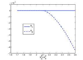
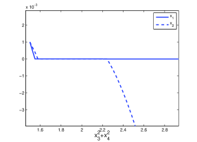
  Figure 2. Example 4.1. Left: Average trajectory obtained with Random Euler and $\tau=10^{-6}$. Right: Regularized Integration, with $\epsilon_{1}=\epsilon_{2}=10^{-5}$ and initial condition $[10^{-3}\,\ 10^{-3}\,\ 0\,\ \sqrt{1.5}]$.

• We also computed the solution of (1.1) with “Deterministic Euler” and fixed stepsize $\tau=10^{-3}$, and initial condition $(10^{-4},10^{-4},0,\sqrt{1.7})$. First, we get rid of the transient and then plot the first two components of the approximation in Figure 3. None of the elements of the sequence generated by the forward Euler’s map is on $\Sigma_{1}$ or $\Sigma_{2}$ and hence the computed solution is always in one of the $R_{j}$’s and the selection of the vector field is straightforward. As it is clear from the plot, we do not recover the dynamics of the original system. The periodic orbit in the $(x_{1},x_{2})$ plane is spurious and is generated by forward Euler’s own dynamics. The periodic orbit survives past the curve of potential tangential exit points and indeed the third and fourth component of the plotted solution are such that $1.5\leq x_{3}^{2}+x_{4}^{2}\leq 30.817$. Notice also that the computed solution is trapped in a neighborhood of $\Sigma$ outside $\gamma$, when $\Sigma$ is not attractive . Periodic motion persists also for smaller values of $\tau$, though the orbit shrinks to the origin as $\tau\to 0$.

• Unregularized integration. Here, this approach works well for relaxed values of the tolerances. To witness, the numerical solution computed with ode23s and RelTol$=$AbsTol=$10^{-7}$, stays close to $\Sigma$ up to $x_{3}^{2}+x_{4}^{2}\simeq 2.0014$. It then leaves $\Sigma$ to slide on $\Sigma_{1}^{-}$. With lower values of RelTol and AbsTol, the integrator takes more than half an hour in the time interval $[0,0.5]$. The integrator ode45 shows a similar behavior.

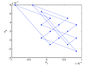
Figure 3. Example 4.1. Numerical solution computed with “Deterministic Euler” and constant stepsize $\tau=10^{-3}$.

Example 4.2 ($\Sigma$ looses attractivity through a non tangential potential exit point).

The vector fields are

(4.2) $$f_{1}=\begin{pmatrix}(3-x_{3})/5\\ -1/5\\ 1\end{pmatrix},\,\ f_{2}=\begin{pmatrix}1/5\\ -1/5\\ 1\end{pmatrix},\,\ f_{3}=\begin{pmatrix}1/5\\ 2/5\\ 1\end{pmatrix},\,\ f_{4}=\begin{pmatrix}-1\\ -1/5\\ 1\end{pmatrix},$$

and $\Sigma$ is the $x_{3}$-axis, with uniquely defined sliding vector field $\dot{x}_{3}=1$. $\Sigma$ is attractive through sliding along $\Sigma_{1}^{+}$ and $\Sigma_{2}^{+}$ for $x_{3}<3$. At $x_{3}=3$, $f_{1}$ is tangent to $\Sigma_{1}$ and points away from $\Sigma$ so that the point $(0,0,3)$ is a potential non tangential exit point. When $x_{3}>3$, the vector field $f_{1}$ points away both from $\Sigma_{1}$ and $\Sigma_{2}$ and we expect the solution of (1.1) to move away from $\Sigma$ and to enter $R_{1}$.

• Random Euler. This behaves qualitatively as we expect. We take $100$ initial conditions uniformly distributed in $[-\tau,\tau]^{2}$. With $\tau=10^{-4}$, the average “exit point” is $\bar{x}=2.9854$ with standard deviation $x_{s}=0.0122$. With $\tau=10^{-5}$, we obtain $\bar{x}=2.9923$, $x_{s}=0.0046$. The average trajectory obtained with stepsize $\tau=10^{-5}$ is plotted in Figure 4. The exit point for the trajectory is $\bar{x}\simeq 2.9944$.

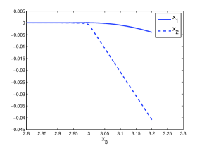
  Figure 4. System (4.2). Average trajectory computed with Random Euler and stepsize $\tau=10^{-5}.$

  

• Regularized Integration. For the regularized vector field (2.2), we take $\alpha$ and $\beta$ as in (2.3), but we make different choices for the parameter $\epsilon$. We use two different parameters for $\alpha$ and $\beta$, namely $\epsilon_{\alpha}=\epsilon_{\beta}=10^{-6}$ and $\epsilon_{\alpha}=10^{-6}$, $\epsilon_{\beta}=10^{-5}$. The corresponding fast systems (2.8) and (2.9) are not orbitally equivalent and, as a consequence of this, the behavior of the regularized solutions differs as well. We first consider the regularized system for $\epsilon_{\alpha}=\epsilon_{\beta}$. In this case, $(\alpha^{*}(x_{3}),\beta^{*}(x_{3}))$ is an asymptotically stable equilibrium of (2.8) in $(0,1)^{2}$ for $x_{3}<\bar{x}_{3}\simeq 3.3853$. For $x_{3}=\bar{x}_{3}$, the eigenvalues of the Jacobian matrix of (2.8) at the equilibrium cross the imaginary axis and $(\alpha^{*}(x_{3}),\beta^{*}(x_{3}))$ undergoes a subcritical Hopf bifurcation. In Figure 5, on the left, we plot both the stable equilibrium and the unstable periodic orbit for (2.8) and $x_{3}=3.8$. The periodic orbit separates the solutions that converge to the equilibrium $(\alpha^{*},\beta^{*})$ from the solutions that reach (possibly in finite time) the boundary of $[0,1]^{2}$. Notice that, if the initial condition of (2.4) satisfies (iii) of Theorem 2.3, then b) in Theorem 2.3 follows, and the regularized solution remains in a neighborhood of $\Sigma$ as long as $(\alpha^{*}(x_{3}),\beta^{*}(x_{3}))$ is attractive. As a consequence of this reasoning, for $\epsilon$ sufficiently small, we expect the solution of (2.4) to remain close to $\Sigma$ up to $x_{3}=\bar{x}_{3}$. For $x_{3}>\bar{x}_{3}$, all solutions inside $(0,1)^{2}$ reach the boundary of the square, and we expect the regularized solution to move away from $\Sigma$. This is well illustrated in the left plot of Figure 7. The equilibrium of (2.10) undergoes a subcritical Hopf bifurcation at $x_{3}=\hat{x}_{3}\simeq 3.4476$. For $x_{3}>\hat{x}_{3}$, all solutions leave the square $[0,1]^{2}$. In the right plot of Figure 5, we show the unstable periodic orbit together with the stable equilibrium for (2.10) with $x_{3}=3.447$.

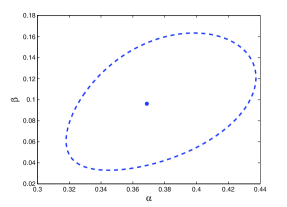
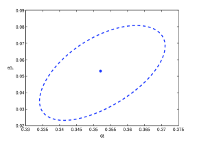
  Figure 5. Example 4.2. Left: unstable periodic orbit and equilibrium $(\alpha^{*},\beta^{*})$ of (2.8) for $x_{3}=3.8$. Right: unstable periodic orbit and equilibrium of (2.10) for $x_{3}=3.447$.

  

  

  With the second set of parameter values, $\epsilon_{\alpha}=10^{-5}$ and $\epsilon_{\beta}=10^{-6}$, the dynamics of (2.9) is similar, but the bifurcation values are different. The equilibrium $(\alpha^{*}(x_{3}),\beta^{*}(x_{3}))$ of (2.9) is stable up to $x_{3}=\bar{x}_{3}\simeq 3.2296$ and at $x_{3}=\bar{x}_{3}$ it undergoes a subcritical Hopf bifurcation. In the left plot of Figure 6 we plot both the unstable periodic orbit and the stable equilibrium of (2.9) for $\epsilon_{\alpha}=10^{-6}$, $\epsilon_{\beta}=10^{-5}$ and $x_{3}=3.22$. We also integrate the fast system backward in time for $x_{3}=3.21$ from an initial condition in a neighborhood of the equilibrium. There is no periodic orbit in this case, since the backward solution meets the boundary of $[0,1]^{2}$ in finite time. The star in the plot marks the equilibrium $(\alpha^{-},0)$ of the fast system. This is the sliding vector field on $\Sigma_{1}^{-}$.

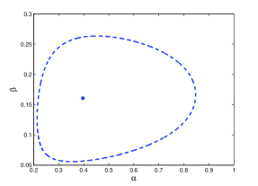
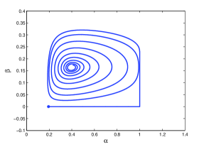
  Figure 6. Example 4.2. Left Plot: unstable periodic orbit and stable equilibrium for the fast system (2.9), $\epsilon_{\alpha}=10^{-6}$, $\epsilon_{\beta}=10^{-5}$ and $x_{3}=3.22$. Right plot: backward trajectory for the fast system for $x_{3}=3.21$.

  

  

  On the left of Figure 7, we plot the numerical solution obtained integrating the regularized problem (2.2), $\dot{x}=f_{B}^{\epsilon}(x)$, with ode23s and RelTol=AbsTol$=10^{-12}$ for $\epsilon_{\alpha}=\epsilon_{\beta}=10^{-6}$. The continuous line is the first component of the solution, while the dotted line is the second component. They are plotted against the third component. The solution stays close to $\Sigma$ up to $x_{3}\simeq 3.39$ and then it enters $R_{1}$. This is in agreement with the singular perturbation analysis. For the second set of parameters, $\epsilon_{\alpha}=10^{-6}$, $\epsilon_{\beta}=10^{-5}$, the numerical solution obtained with ode23s remains close to $\Sigma$ up to $x_{3}\simeq 3.369$, and this is not in agreement with the singular perturbation analysis. The numerical solution obtained with ode15s is even less accurate and exits at $x_{3}\simeq 3.485$. We integrated the problem also with lower values of $\epsilon_{\beta}$, while still having $\epsilon_{\alpha}=\frac{\epsilon_{\beta}}{10}$ so that the corresponding fast systems are all equivalent. The numerical approximations are even less reliable, and indeed the computed exit values increase as $\epsilon_{\beta}$ decreases. On the other hand, the numerical solution computed with ode45 behave more reliable leaves $\Sigma$ to enter $R_{1}$ for $x_{3}\simeq 3.238$, as we can see from the right plot in Figure 7.

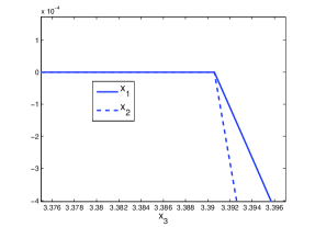
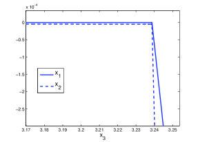
  Figure 7. Example 4.2. Solution of the regularized system (2.2) with ode45. Left: $\epsilon_{\alpha}=\epsilon_{\beta}=10^{-6}$. Right: $\epsilon_{\alpha}=10^{-6}$ and $\epsilon_{\beta}=10^{-5}$.

Example 4.3 (Spiral dynamics around $\Sigma$).

In this example the vector fields are

(4.3) $$f_{1}=\begin{pmatrix}\frac{1}{3}\\ -\frac{x_{3}}{3}\\ 1\end{pmatrix},\,\ f_{2}=\begin{pmatrix}-\frac{2}{3}\\ -1\\ 1\end{pmatrix},\,\ f_{3}=\begin{pmatrix}\frac{1}{3}\\ \frac{2}{3}\\ 1\end{pmatrix},\,\ f_{4}=\begin{pmatrix}-\frac{1}{3}\\ 1\\ 1\end{pmatrix}.$$

$\Sigma$ is the $x_{3}$-axis, with uniquely defined Filippov sliding motion $\dot{x}_{3}=1$, and there is spiral like dynamics around $\Sigma$. For $x_{3}<1$, $\Sigma$ is attractive in finite time while, for $x_{3}>1$, $\Sigma$ is not locally attractive.

• Random Euler. Approximations computed with “Random Euler” move away from $\Sigma$ for $x_{3}>1$. In Figure 8 we show the average trajectory computed with $\tau=10^{-5}$ and initial condition $(10^{-6},10^{-6},0.5)$.

  Figure 8. Example 4.3. Average trajectory obtained with Random Euler and $\tau=10^{-5}$.

  For a statistical estimate of the exit point, we consider an ensamble of $100$ initial conditions with the first two components uniformly distributed in $[-\tau,\tau]^{2}$. For $\tau=10^{-5}$, the mean value of $x_{3}$ at the exit point is $\bar{x}_{3}\simeq 0.94777$, with standard deviation $\simeq 0.04297$. For $\tau=10^{-6}$, the mean value of $x_{3}$ at the exit point is $\bar{x}_{3}\simeq 0.97910$ and the standard deviation is $\simeq 0.00529$. In Figure 9, on the left, we plot a trajectory of (1.1) obtained with Random Euler and stepsize $\tau=10^{-6}$. On the right of Figure 9 we plot the $2$-norm of the vector $(h_{1},h_{2})$ (for us, this is the vector $(x_{1},x_{2})$) in function of $x_{3}$. The “X” in the plot marks the estimated exit point.

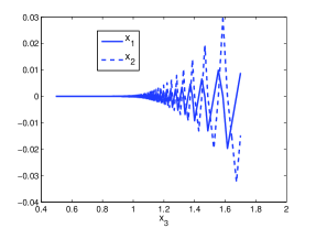
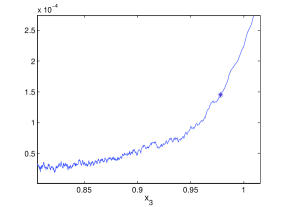
  Figure 9. Example 4.3. Left: a solution of (4.3) obtained with Random Euler and $\tau=10^{-5}$. Right: norm of the vector $(h_{1},h_{2})$ in function of $x_{3}$ for this trajecytory.

• Regularized Integration. Next, consider integrating the regularized vector field (2.2) with $\alpha$ and $\beta$ as in (2.3) and two different sets of parameters. We first consider $\epsilon_{\alpha}=\epsilon_{\beta}=10^{-4}$. For these parameters values, the equilibrium $(\alpha^{*},\beta^{*})$ of the fast system (2.8) is stable up to $x_{3}\simeq 1.41798$, then the eigenvalues of the Jacobian matrix at the equilibrium cross the imaginary axis. We compute the solution of the regularized system with initial condition $(10^{-4},10^{-4},0)$ in the time interval $[0,2]$ (so that $0\leq x_{3}\leq 2$) with ode23s, ode15s and ode45 with RelTol=AbsTol$=10^{-12}$. The computed solutions show different behavior: the numerical solution computed with ode23s and ode15s remain in a small neighborhood of $\Sigma$ for the whole time interval $[0,2]$, while the solution computed with ode45 moves away from $\Sigma$ for $x_{3}\simeq 1.5$ as it is seen from the left plot of Figure 10. The average stepsize used by the stiff integrators is $O(10^{-2})$, while the one used by the explicit integrator is $O(10^{-4})$. We then consider a second set of parameters $\epsilon_{\alpha}=10^{-4}$ and $\epsilon_{\beta}=10^{-3}$. The equilibrium $(\alpha^{*},\beta^{*})$ of the corresponding fast system (2.9) is unstable when $x_{3}>0$. On the right of Figure 10 we plot the approximation computed with ode23s (the approximation computed with ode45 behaves in a similar way).

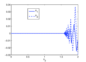
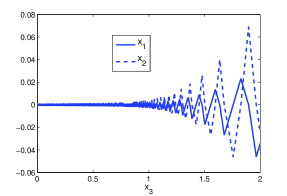
  Figure 10. Example 4.3. Regularized integration with ode23s. Left: $\epsilon_{\alpha}=\epsilon_{\beta}=10^{-4}$. Right: $\epsilon_{\alpha}=10^{-4}$ and $\epsilon_{\beta}=10^{-3}$.

• Unregularized integration. The numerical solution obtained with the stiff Matlab integrator ode23s, with RelTol$={\tt AbsTol}=10^{-7}$, stays close to $\Sigma$ up to $x_{3}=1$ and then it leaves $\Sigma$ to enter one of the $R_{j}$’s. For lower values of RelTol, the integrator takes more than half an hour in the time interval $[0,1]$. The numerical solution obtained with ode15s and RelTol=AbsTol=$10^{-6}$ is very inaccurate as it is evident from the plot in Figure 11. Lower tolerances do not produce better results.

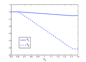
  Figure 11. Example 4.3. Unregularized integration with ode15s and RelTol=AbsTol=$10^{-6}$.

  

Example 4.4 (Filippov’s vector field on $\Sigma$ is ambiguous).

We consider the following vector fields

(4.4) $$\begin{split}f_{1}=\begin{pmatrix}\frac{1}{2}\\ 1\\ -x_{3}+\frac{1}{2}x_{4}\\ x_{4}\end{pmatrix},\qquad\qquad f_{2}=\begin{pmatrix}1\\ \frac{1}{2}\\ -x_{3}+\frac{1}{2}x_{4}\\ x_{4}\end{pmatrix}\\ f_{3}=\begin{pmatrix}-(x_{3}-3)^{2}-(x_{4}-3)^{2}+5\\ 1\\ -x_{3}+28x_{4}\\ x_{4}\end{pmatrix},\,\ f_{4}=\begin{pmatrix}-1\\ -1\\ -x_{3}+4x_{4}\\ x_{4}\end{pmatrix},\end{split}$$

and $\Sigma$ is the $(x_{3},x_{4})$ plane. The circle $\gamma=\{x\in\mathbb{R}^{4},(x_{3}-3)^{2}+(x_{4}-3)^{2}=4\}$ (see Figure 12), divides $\Sigma$ in two regions. Outside $\gamma$, $\Sigma$ is attractive upon sliding along $\Sigma_{1}^{+}$ and $\Sigma_{2}^{+}$. For all points on $\gamma$, the vector field $f_{\Sigma_{2}}^{+}$ is tangent to $\Sigma$ and, inside $\gamma$, it points away from $\Sigma$, so that $\Sigma$ is not attractive from inside  $\gamma$. We would expect the solution of (1.1) to leave $\Sigma$ once it reaches $\gamma$. Note that there is a family of Filippov sliding vector fields on $\Sigma$, namely: $\dot{x}_{1}=\dot{x}_{2}=0$, $\dot{x}_{3}=-x_{3}+(16-13\lambda)x_{4}$, $\dot{x}_{4}=x_{4}$, with $0\leq\lambda\leq\frac{2}{7}$.

• Random Euler. The ambiguity of a Filippov sliding vector field is clearly reflected in the numerical solutions computed with Random Euler. In Figure 12 we plot the $x_{3}$ and $x_{4}$ components of $1000$ trajectories computed with $\tau=10^{-2}$, and same initial condition $(10^{-2},10^{-2},3,0.9)$. The dotted circle in the plot is the curve $\gamma$. The two bold darker lines are two sample trajectories. The shaded region is obtained by plotting all $1000$ trajectories. The plot suggests that the choice of random stepsizes covers the region obtained by choosing one of the possible vector fields in Filippov’s differential inclusion.

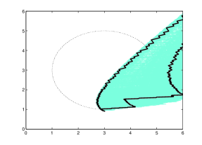
  Figure 12. Example 4.4: plot in the plane $(x_{3},x_{4})$ of $1000$ approximations obtained with Random Euler and $\tau=10^{-2}$, and initial condition $(10^{-2},10^{-2},3,0.9)$.

  

  For completeness, in Figure 13 we plot in function of time the first and second component of the average trajectory computed with Random Euler with $\tau=10^{-5}$. At $t\simeq 0.1067$, the third and fourth components of the average trajectory are on $\gamma$ and indeed the plotted solution leaves $\Sigma$ and starts sliding on $\Sigma_{2}^{+}$ at $t\simeq 0.12$.

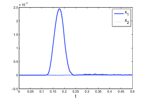
  Figure 13. Example 4.4. First and second component of the numerical solution computed with Random Euler with $\tau=10^{-5}$.

  

• Regularized Integration. Here, the computed approximations of the regularized system move away from $\Sigma$ once they reach $\gamma$. We note that $\gamma$ is a curve of saddle-node bifurcation values for (2.8) for any parameter value $\epsilon_{\alpha}$ and/or $\epsilon_{\beta}$. On $\gamma$, $(\alpha^{*},\beta^{*})=(1,0.5)$ is a double root of (2.7), while inside $\gamma$ there is no solution of (2.7).

5. Conclusions

In this work we have been interested in studying the behavior of solutions of piecewise smooth systems in the neighborhood of a co-dimension $2$ discontinuity surface $\Sigma$, intersection of two co-dimension $1$ discontinuity surfaces. It has long been accepted that if solution trajectories cannot leave $\Sigma$ ($\Sigma$ is attractive), some form of sliding motion on $\Sigma$ should be taking place. Precisely which sliding motion has been the subject of much investigation, but it has not been our concern in this paper. Our chief interest in this work has been trying to understand what should happen when $\Sigma$ loses attractivity (at generic first order exit points). To our knowledge, this type of study had not been carried out before.

We took the point of view that the piecewise smooth system (1.1) was the only information at our disposal, and treated this model with its own mathematical dignity. Naturally, if (1.1) arose as a simplified model for some other known differential system, then this original system should ultimately guide the search for appropriate dynamics near $\Sigma$, and it may well be that the dynamics of this “true” system are not matched by those of (1.1). If this is the case, we should legitimately question the validity of the model (1.1) in the first place. On the other hand, in the absence of knowledge of an underlying “true” system, when (1.1) is the only datum we have, then we believe that we should try to modify this model so that the dynamics of the modified system match those of (1.1).

To obtain information on the dynamics of (1.1), we proposed use of a simple Euler method with random steps, uniformly chosen with respect to a reference, small, stepsize. Our study unambiguously show that: (i) when $\Sigma$ is attractive, solution trajectories remain near $\Sigma$ (thereby validating an idealized sliding motion on $\Sigma$); (ii) when $\Sigma$ loses attractivity, solution trajectories leave a neighborhood of $\Sigma$.

Several other possibilities have also been considered in this work: regularization techniques, plain and simple Euler method with fixed stepsize, and direct numerical integration of (1.1) with sophisticated off-the-shelf solvers for differential equations. None of these options satisfactorily resolved the dynamics of (1.1), and often produced misleading behavior. Ultimately, this occurred because each of these choices either superimposed its own dynamics on those of (1.1) (as Euler method and regularization techniques do, further producing different behaviors depending on how the regularization is made), or just failed to produce reliable answers in too many cases (this was the case with directly solving (1.1) with existing software, where the outcome dramatically dependend on the solver used, or on the tolerances values, or both).

Unfortunately, our conclusions are not fully satisfactory either. Our analysis tells us that is the dynamics of (1.1) around $\Sigma$ that must be used to tell us what should happen in a neighborhood of $\Sigma$, but we know of no general foolproof mean to regularize the system so that the regularized trajectory will be following the dynamics of (1.1). Perhaps, and –again– as long as the model (1.1) is appropriate, the most reliable and practically efficient way to proceed is to accept some form of idealized sliding motion on $\Sigma$ as long as $\Sigma$ is attractive, while also demanding that a sliding trajectory leaves $\Sigma$ when the latter loses its attractivity. The construction of appropriate sliding vector fields fulfilling these requests remains an outstanding and challenging task.

References

- [1] J.C. Alexander and T. Seidman, Sliding modes in intersecting switching surfaces, I: Blending. Houston J. Math., 24:545–569, 1998.
- [2] J.C. Alexander and T. Seidman, Sliding modes in intersecting switching surfaces, II: Hysteresis. Houston J. Math., 25:185–211, 1999.
- [3] Z. Artstein, On singularly perturbed ordinary differential equations with measure-valued limits Mathematics Bohemica, 2: 27-31, 2001.
- [4] J. Cortes, Discontinuous Dynamical Systems: A tutorial on solutions, nonsmooth analysis, and stability IEEE Control Systems Magazine, 28-3:36–73, 2008.
- [5] N. Del Buono, C. Elia and L. Lopez On the equivalence between the sigmoidal approach and Utkin’s approach for models of gene regulatory networks SIAM J. Applied Dynamical Systems, 13-3 (2014), pp. 1270-1292.
- [6] M. di Bernardo, C.J. Budd, A.R. Champneys, and P. Kowalczyk, Piecewise-smooth Dynamical Systems. Theory and Applications. Applied Mathematical Sciences 163. Springer-Verlag, Berlin, 2008.
- [7] L. Dieci, Sliding motion on the intersection of two manifolds: Spirally attractive case. Communications in Nonlinear Science and Numerical Simulation, 26 (2015), pp. 65-74
- [8] L. Dieci, and F. Difonzo, A Comparison of Filippov sliding vector fields in co-dimension . Journal of Computational and Applied Mathematics, 262 (2014), 161-179. Corrigendum in Journal of Computational and Applied Mathematics, 272 (2014), pp. 273-273.
- [9] L. Dieci, and F. Difonzo, The Moments sliding vector field on the intersection of two manifolds. Journal of Dynamics and Differential Equations, to appear, 2015. DOI 10.1007/s10884-015-9439-9
- [10] L. Dieci, C. Elia, and L. Lopez, A Filippov sliding vector field on an attracting co-dimension 2 discontinuity surface, and a limited loss-of-attractivity analysis. J. Differential Equations, 254, (2013), pp. 1800–1832.
- [11] L. Dieci, C. Elia, and L. Lopez, Sharp sufficient attractivity conditions for sliding on a co-dimension 2 discontinuity surface. Mathematics and Computers in Simulations 110-1, (2015), pp. 3–14.
- [12] L. Dieci, C. Elia, and L. Lopez, Uniqueness of Filippov sliding vector field on the intersection of two surfaces in and implications for stability of periodic orbits. J. Nonlin. Science, to appear JNLS-D-14-00195.1 (2015), DOI: 10.1007/s00332-015-9265-6.
- [13] L. Dieci and N. Guglielmi Regularizing piecewise smooth differential systems: co-dimension 2 discontinuity surface. J. Dynamics and Differential Equations, 25:1, 71–94, 2013.
- [14] A. Dontchev and F. Lempio, Difference methods for differential inclusions: a survey. SIAM REVIEW, 34, No. 2, (1992), pp. 263-294.
- [15] A.F. Filippov, Differential Equations with Discontinuous Right-Hand Sides. Mathematics and Its Applications, Kluwer Academic, Dordrecht, 1988.
- [16] N. Guglielmi and E. Hairer Classification of hidden dynamics in discontinuous dynamical systems SIADS, in press.
- [17] M. Jeffrey, Dynamics at a switching intersection: hierarchy, isonomy, and multiple sliding, SIAM J. Applied Dyn. Systems, 13:1082-1105, 2014.
- [18] J. Llibre, P. R. Silva, and M. A. Teixeira, Regularization of discontinuous vector fields on via singular perturbation. J. Dynam. Differential Equations, 19:309–331, 2007.
- [19] A. Machina, R. Edwards, and P. van den Driessche, Singular dynamics in gene network models SIAM J. Appl. Dyn. Syst., 12 (1): 95–125, 2013.
- [20] E. Plahte, and S. Kjóglum, Analysis and generic properties of gene regulatory networks with graded response functions Physica D, 201 (1): 150–176, 2005.
- [21] A. Polynikis, S.J. Hogan, and M. di Bernardo, Comparing different ODE modelling approaches for gene regulatory networks, Journal of Theoretical Biology, 261(4): 511–530, 2009.
- [22] T. Seidman, Some limit results for relays. Proc.s of World Congress of Nonlinear Analysts, Volume 1. Ed. V. Lakshmikantham, De Gruyter publisher (1996), pp. 787–796.
- [23] T. Seidman, The residue of model reduction. The residue of model reduction, In Hybrid Systems III. Verification and Control, Lecture Notes in Comp. Sci. 1066; R. Alur, T.A. Henzinger, E.D. Sontag, eds. pp. 201-207, Springer-Verlag, Berlin (1996).
- [24] J. Sotomayor and Teixeira M.A., Regularization of discontinuous vector field. In International Conference on Differential Equations, pp. 207–223, 1996.
- [25] V.I. Utkin, Sliding Modes and Their Application in Variable Structure Systems. MIR Publisher, Moskow, 1978.
- [26] V.I. Utkin, Sliding Mode in Control and Optimization. Springer, Berlin, 1992.