Gene expression dynamics with stochastic bursts:
exact results for a coarse-grained model

Abstract

We present a theoretical framework to analyze the dynamics of gene expression with stochastic bursts. Beginning with an individual-based model which fully accounts for the messenger RNA (mRNA) and protein populations, we propose a novel expansion of the master equation for the joint process. The resulting coarse-grained model reduces the dimensionality of the system, describing only the protein population while fully accounting for the effects of discrete and fluctuating mRNA population. Closed form expressions for the stationary distribution of the protein population and mean first-passage times of the coarse-grained model are derived and large-scale Monte Carlo simulations show that the analysis accurately describes the individual-based process accounting for mRNA population, in contrast to the failure of commonly proposed diffusion-type models.

Intrinsic noise originating from the discreteness of interacting particles plays an important role in genetic expression: it diversifies the distribution of protein population, promotes transition between different cellular phenotypes on a population level, and in turn enhances organisms’ ability to adapt to changing environments without the need of genetic mutation Kaern et al. (2005). There are two primary sources of intrinsic noise in the context of gene expression: transcriptional noise from the stochastic transition between active and repressed states of DNA transcription, and translational noise from the relatively fast action of mRNA to produce the proteins Kaern et al. (2005); Walczak et al. (2011). Both steps result in bursts of protein production which are experimentally observed Ozbudak et al. (2002); Blake et al. (2003).

Many stochastic models have been proposed to model gene circuits Kepler and Elston (2001); Hornos et al. (2005); Walczak et al. (2005); Warren and ten Wolde (2005); Wang et al. (2010a, b); Assaf et al. (2011); Strasser et al. (2012); Zhou et al. (2012); Lu et al. (2014) but only a few studies quantitatively account for the effects of bursting noise Thattai and van Oudenaarden (2001); Friedman et al. (2006); Assaf et al. (2011); Strasser et al. (2012). To our knowledge, current theoretical investigation of the dynamical properties of such bursting processes is limited to stationary properties of the protein distribution on the population level Thattai and van Oudenaarden (2001); Friedman et al. (2006).

This Letter presents a new mathematical framework to analyze bursting noise in gene expression. Starting from an individual-based model including both mRNA and protein populations we construct a novel coarse-grained process describing only the protein population dynamics that fully accounts for the discreteness effects and fluctuations in the mRNA population. When the mRNA degrades at a much shorter time scale, the approximating process converges to currently proposed bursting models Thattai and van Oudenaarden (2001); Friedman et al. (2006). In our process-based framework, mean first-passage times in a autoregulated gene circuit with stochastic bursts can be formulated and calculated.

We present analytic solutions along with computational verification from large-scale Monte-Carlo simulations. A key conclusion is that the conventional diffusion approximation of the master equation fails to accurately estimate switching times of the individual-based model.

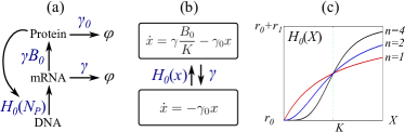
Figure 1: Schematic diagrams of (a) the individual-based model and (b) the piecewise deterministic Markov process model (3). (c) Hill functions with Hill coeffcients $n=1,2,4$.

A simple individual-based model of autoregulated gene expression including both the mRNA and protein populations contains four reaction steps Thattai and van Oudenaarden (2001); Walczak et al. (2011) as summarized in Fig. 1(a): synthesis of mRNA’s (transcription, $\phi\xrightarrow{H_{0}\left(N_{\rm P}\right)}{\rm mRNA}$), production of the protein (translation, ${\rm mRNA}\xrightarrow{\gamma B_{0}}{\rm mRNA}+{\rm Protein}$), and degradation of both the mRNA’s and proteins (${\rm mRNA}\xrightarrow{\gamma}\phi$ and ${\rm Protein}\xrightarrow{\gamma_{0}}$). In the first step $N_{\rm P}$ is the random number of available proteins and in this autoregulated genetic circuit, the population of proteins regulates the transcription rate. The Hill function $H_{0}(X):=r_{0}+r_{1}X^{n}/(K^{n}+X^{n})$ with the Hill coefficient $n$ approximates the autoregulated transcription rate when the gene switches between on and off states on a much shorter time scale Walczak et al. (2011).

We refer to the process in Fig. 1(a) as the individual-based (IB) model. Although the IB model provides a detail description of both the mRNA and protein populations, it is generally difficult to analyze theoretically except for linear cases Shahrezaei and Swain (2008); Kumar et al. (2014). Single-species models describing only the protein populations are often adopted, especially for more complicated genetic circuits Wang et al. (2010b); Zhou et al. (2012); Wang et al. (2010a); Lu et al. (2014). However, fluctuations in the mRNA population are an important dynamical factor Assaf et al. (2011); Strasser et al. (2012) and our objective is to construct a coarse-grained model describing only the protein population accounting for contributions from fluctuation in the mRNA population.

Generally mRNA’s degrade much faster than proteins. In the model organism Escherichia coli for example, the mean lifetime of the mRNA is about $2\min$ while protein lifetimes are $45\sim 60\min$ Thattai and van Oudenaarden (2001). As a consequence, a large number of proteins is produced in a relatively short period of time—a phenomenon termed translational bursting. In addition, due to small system size (the volume of E. coli are $\sim 10^{-18}{\rm m}^{3}$), the onset of the transcription and the lifetime of the synthesized mRNA are observed in a stochastic manner Cai et al. (2006).

Motivated by the observation of translational bursting, we propose a novel expansion to approximate the master equation of the IB process in Fig. 1(a). First, we notice that in the IB model, for any given mRNA number $m$, the protein population $N_{P}(t)$ is a birth-death processes with constant birth rate $m\gamma B_{0}$ and constant per capita death rate $\gamma_{0}$. Therefore, it is convenient to expand the process describing the protein dynamics conditioning on the mRNA population: each “state” of the system is labeled by the mRNA number $m$. The transition rate from state $m$ to $m+1$ mRNA molecules is the autoregulated transcription rate $H_{0}(N_{P})$, and the transition rate from state $m+1$ to $m$ mRNA molecules is the mRNA degradation rate $\gamma$. Within each state of the system we perform a Kramers–Moyal expansion of the birth-death process van Kampen (2007); Kurtz (1971) with respect to the system size $K\gg 1$. In the lowest order approximation only the advection terms describing the mean-field dynamics are retained Kurtz (1970). Formally letting the protein concentration be $x:=N_{\text{P}}/K\geq 0$ and the number of mRNA molecules be $m\in\left\{0,1,2,\ldots\right\}$, in each state the protein density evolves according to the deterministic equation

$$\dot{x}(t)=m\gamma\frac{B_{0}}{K}-\gamma_{0}x,$$ (1)

with transition rates between different states

$$m\xrightarrow{H(x)}m+1\text{ and }m\xrightarrow{\gamma}m-1$$ (2)

where $H(x):=H_{0}(Kx)$ is the scaled Hill-function.

Next we note that the mean lifetime of the mRNA is $\mathcal{O}(1/\gamma)$ and in the fast-degrading mRNA limit $\gamma\gg 1$, most of the time the system has either $m=0$ or $m=1$. We therefore neglect states $m\geq 2$ and formulate a closed forward equation for $p_{m}(x,t)$, the joint probability density that the system presents $m\in\left\{0,1\right\}$ mRNA molecules and protein density $x$ at time $t$:

$$\frac{\partial}{\partial t}\left(\begin{array}[]{c}p_{1}(x,t)\\ p_{0}(x,t)\\ \end{array}\right)=L^{\dagger}\left(\begin{array}[]{cc}p_{1}(x,t)\\ p_{0}(x,t)\\ \end{array}\right),$$ (3)

where the forward operator is defined to be

$$L^{\dagger}:=\left(\begin{array}[]{cc}-\gamma-\partial_{x}\left(\gamma b-\gamma_{0}x\right)&H(x)\\ \gamma&-H(x)+\gamma_{0}\partial_{x}x\\ \end{array}\right)$$ (4)

where we have defined $b:=B_{0}/K$ to be a dimensionless parameter characterizing the strength of the bursts. We shall refer to (3) as the piecewise deterministic Markov process (PDMP; schematic diagram Fig. 1(b)) and remark that the process in $x$ alone is non-Markovian.

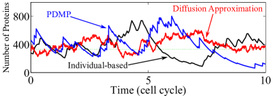
Figure 2: Sample paths of the models. Dotted green line denotes 165 molecules which separates low and high protein abundance mode.

To proceed with our analytic investigation, an infinitely fast-degrading mRNA limit $\gamma\rightarrow\infty$ is taken. Although in such a limit the mean duration when the system stays in $m=1$ state is $1/\gamma\rightarrow 0$, the protein concentration in $m=1$ state increases with a rate $b\gamma\rightarrow\infty$, preserving exponentially distributed random burst with an average burst strength $b$. In this limit the process stays in $m=0$ state almost surely (i.e. $p_{1}(x,t)\rightarrow 0\ \forall t$), and the probability distribution $p_{0}$ satisfies a closed and second-order differential equation

$$\left(1+b\partial_{x}\right)\partial_{t}p_{0}=-\partial_{x}\left[-x+bH(x)-b\gamma_{0}\partial_{x}x\right]p_{0}.$$ (5)

The stationary probability distribution is obtained by direct integration:

$$p_{\rm stat}(x)=\frac{{\cal N}}{\gamma_{0}x}\,\exp\left\{\frac{-x}{b}+\int^{x}{\frac{H(\xi)d\xi}{\gamma_{0}\xi}}\right\}$$ (6)

where $\cal N$ is the normalization factor. Substituting the explicit form of the Hill function we find the analytic expression for the stationary distribution

$$p_{\rm stat}(x)=\frac{\cal N}{\gamma_{0}}e^{-\frac{x}{b}}x^{\frac{r_{0}}{\gamma_{0}}-1}\left(x^{n}+1^{n}\right)^{\frac{r_{1}}{n\gamma_{0}}}.$$ (7)

We remark that in the limit $\gamma\rightarrow\infty$ the PDMP model reduces to the bursting model described by a continuous master equation, and that this result confirms Friedman et al. (2006).

In some parameter regimes the stationary distribution (7) exhibits bi-stability Horsthemke and Lefever (2006) and can be adopted to model a biological switch Friedman et al. (2006); Assaf et al. (2011). Our formulation (3) can be used to derive the mean switching time (MST) between two modes of gene expression in a straightforward way Doering (1986). We begin by deriving the mean first-exit time to leave a domain $(x_{1},x_{2})$ where $0<x_{1}<x_{2}<\infty$.

If the initial protein concentration is $x\in(x_{1},x_{2})$ and the initial number of mRNA is $m$, then the mean time to exit the domain $T_{m}(x)$ satisfies the inhomogeneous equation van Kampen (2007)

$$-\left(\begin{array}[]{cc}1\\ 1\\ \end{array}\right)=L\left(\begin{array}[]{cc}T_{1}(x,t)\\ T_{0}(x,t)\\ \end{array}\right),$$ (8)

where the generator $L$ is the adjoint of the forward operator in (4),

$$L=\left(\begin{array}[]{cc}-\gamma+\left(\gamma b-\gamma_{0}x\right)\partial_{x}&\gamma\\ H(x)&-H(x)-\gamma_{0}x\partial_{x}\\ \end{array}\right)$$ (9)

with boundary conditions

$$T_{1}(x_{2})=0,\,T_{0}(x_{1})=0.$$ (10)

The physical meaning of the boundary conditions is clear: when the system starts with the state $m=1$—a state with fast production of proteins—at upper boundary $x_{2}$, and when the state $m=0$—a state with only degrading proteins—at lower boundary $x_{1}$, immediately the flow leaves the domain $(x_{1},x_{2})$.

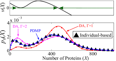
Figure 3: Top panel: Drift of the mean-field dynamics $\dot{x}=bH(x)-\gamma_{0}x$ showing a single fixed point. Bottom panel: Stationary probability distributions of individual-based model, piecewise deterministic Markov process (PDMP), and the diffusion approximations (DA). Solid lines are analytic solutions. Discrete markers represent numerically measured probability distributions from Monte Carlo simulations.

Taking the limit $\gamma\rightarrow\infty$ we deduce a closed second-order differential equation for $T_{0}$,

$$-T^{\prime\prime}_{0}-\left[\frac{H}{f}-\frac{1}{b}+\frac{H}{x}\left(\frac{x}{H}\right)^{\prime}\right]T^{\prime}_{0}=\frac{1}{b\gamma_{0}x}+\frac{H^{\prime}}{\gamma_{0}xH}$$ (11)

where prime denote derivative with respect to $x$. The boundary conditions for (11) follow from (10):

$$T_{0}\left(x_{1}\right)=0,1=H\left(x_{2}\right)T_{0}\left(x_{2}\right)+\gamma_{0}x_{2}T_{0}^{\prime}\left(x_{2}\right).$$ (12)

We remark that while formally deriving the backward equations of the bursting models Thattai and van Oudenaarden (2001); Friedman et al. (2006) considering only the protein concentration is possible, imposing the correct boundary conditions (12) is not trivial.

The solution (derived in the Supplemental Material) is

$$T_{0}(x)=C\int_{x_{1}}^{x}e^{-M(y)}dy+\int_{x_{1}}^{x}e^{-M(y)}V(y)dy,$$ (13)

where the auxiliary functions $M(x)$ and $V(x)$ and the constant $C$ are

$$M(x):={} \int^{x}\left[\frac{H(y)}{f(y)}-\frac{1}{b}+\frac{d}{dy}\left(\ln\frac{y}{H(y)}\right)\right]dy,$$ (14)

$$V(x):={} \int^{x}\left(\frac{-1}{b\gamma_{0}y}+\frac{-1}{\gamma_{0}yH(y)}\frac{dH(y)}{dy}\right)e^{M(y)}dy,$$ (15)

$$C\equiv\left[-V(x_{2})e^{-M(x_{2})}f(x_{2})-H(x_{2})\int_{x_{1}}^{x_{2}}V(y)e^{-M(y)}dy+1\right]\left[f(x_{2})e^{-M(x_{2})}+H(x_{2})\int_{x_{1}}^{x_{2}}e^{-M(y)}dy\right]^{-1}.$$ (16)

This solution is a generalization of results in Masoliver et al. (1986); Doering (1987).

When the system exhibits bi-modality, the mean switching times between two modes of protein expression can be obtained by taking appropriate limits of (13). First, we define a critical density $x_{c}$ separating the low and high protein abundance modes, then take $x_{1}\rightarrow 0$ and $x_{2}\rightarrow x_{c}$ for the low mode, and $x_{1}\rightarrow x_{c}$ and $x_{2}\rightarrow\infty$ for the high mode. Careful analysis is needed because (11) is singular at $x=0$ (and is presented in the Supplemental Material). The analytic expressions for the mean switching times (MSTs) are

$$T_{\rm low\rightarrow high}\equiv{} \int_{0}^{x}e^{-M(y)}V(y)dy+C_{2},$$ (17)

$$T_{\rm high\rightarrow low}\equiv{} \int_{x_{c}}^{x}e^{-M(y)}\left[V(y)-V(\infty)\right]dy,$$ (18)

where the constant $C_{2}$ is

$$C_{2}:=\frac{1-x_{c}V(x_{c})e^{-M(x_{c})}}{H(x_{c})}-\int_{0}^{x_{c}}e^{-M(y)}V(y)dy.$$ (19)

We now turn to the diffusion approximation (DA) of the IB process. To our knowledge there is no standard way to derive DA models for general bursting kernels. In the Supplemental Material we present the straightforward Kramers–Moyal expansion van Kampen (2007); Kurtz (1971) of the master equation of the IB process in the limit $\gamma\rightarrow\infty$ yielding the Itô stochastic differential equation

$$dX_{t}=\left[bH(X_{t})-\gamma_{0}X_{t}\right]dt+\sqrt{\Gamma b^{2}H\left(x\right)}\,dW_{t}$$ (20)

where $X_{t}$ is the random population density of the proteins, $W_{t}$ is the standard Wiener process and the scaling factor $\Gamma=2$. An alternative and phenomenological construction the diffusion approximation is to insert the mean and variance of the bursting kernel in the individual-based process (see Supplemental Material) which yields (20) with the scaling factor $\Gamma=1$. To avoid leaking probabilities to negative densities, we put a reflective boundary at the origin $x=0$. Analytic expressions for the stationary distribution and the mean switching times of the diffusion equation are derived by standard analysis van Kampen (2007) and presented in the Supplemental Material.

We performed numerical simulations to measure the stationary distributions and the mean switching times (MST) in all three models to verify the theoretical analysis. For the IB model, exact sample paths are generated by standard continuous time Markov chain simulations Schwartz (2008). For the PDMP model, kinetic Monte Carlo simulations can be constructed by generating exact random waiting times to the next transition events . In the limit $\gamma\rightarrow\infty$, we adopted a previously proposed algorithm Bokes et al. (2013). For the diffusion approximations we construct a standard Euler–Maruyama integrator of (20).

The parameters were chosen to be in a biologically relevant regime Friedman et al. (2006); Thattai and van Oudenaarden (2001); Taniguchi et al. (2011): $K=200$, $n=4$, $B_{0}=40$, $r_{0}=2$, $r_{1}=10$, $\gamma=30$, while $\gamma_{0}:=1$ is chosen to normalize the unit of the time by a natural cell cycle.

Fig. 3 presents the stationary probability distributions of the IB, PDMP, and DA models. Note that the low-mode is noise induced and does not exist in the mean-field dynamics (top panel of Fig 3). While the PDMP model captures the stationary distribution of the IB model extremely well, directly expanding the IB stochastic bursting model by Kramers–Moyal expansion (DA with $\Gamma=2$) qualitatively captures the stationary distribution, and the phenomenological DA model with $\Gamma=1$ failed to capture the stability of the low mode.

Fig. 4 presents the MST between low and high protein-abundance modes in all three models. Again, the PDMP model well estimates the mean switching times of the IB model, and both the DA models fail by a large amount. When the state is initially below $x_{c}$, both the DA models under-estimate the transition time because the bursting kernels of the DA model have a thinner (Gaussian) tail compared to to the geometric (for the derivation see Supplemental Material) bursting kernel of the IB model. When the initial state is above $x_{c}$, the DA model with $\Gamma=1$ over-estimate the MST because the the approximation does not capture the high probabilities of low-density bursts, and the DA model with $\Gamma=2$ underestimate the MST because the approximation fail to capture that the bursting kernel is always positive.

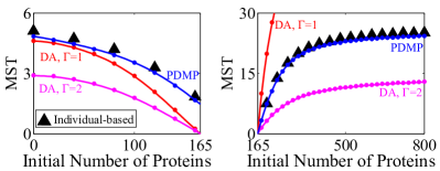
Figure 4: Mean switching times (MST) of the individual-based model, piecewise deterministic Markov process (PDMP), and the diffusion approximations (DA). Solid lines are analytic predictions, and discrete markers are measured from Monte Carlo simulations. Left panel: $T_{\rm low\rightarrow high}$; Right panel: $T_{\rm high\rightarrow low}$. $x_{c}:=165/K$.

The PDMP approximation works well even for models with a strong noise strength. In our example, the low-mode is of an order of $100$ protein molecules, and the noise strength (per each burst) is of order $40$ protein molecules. In addition, the PDMP approximation performs well even though an infinitely-fast degrading mRNA limit $\gamma\rightarrow\infty$ is taken and consequently almost surely there is no mRNA presented in the system. Meanwhile we observe an average $0.3188$ mRNA in the stationary state of the IB model.

The PDMP model can be easily generalized. For example, finite population and lifetime of mRNA can be considered by generalize (3) to include $p_{m}$ with $m\in\left\{0,1,2,\ldots\right\}$. The transcriptional bursting can be included by considering multiple stages of the gene. Higher dimensional genetic circuit can be investigated by including more states of the system Lin and Galla (2015). These generalizations merit future investigations.

We conclude that bursting originating from the discreteness of the fast-living mRNA molecules and the stochastic transcription events is the dominating noise in individual-based autoregulated gene expression model. Diffusion approximations are no longer adequate to analyze the dynamical properties of bursting systems while the novel expansion described here faithfully captures the dynamical properties of the individual-based model in a biologically realistic parameter regime and serves as a new analytic tool to investigate more complex models with bursting noise.

Acknowledgement. YTL was supported by the visitor program at MPI-PKS and EPSRC (grant reference EP/K037145/1). CRD was supported in part by US-NSF Awards PHY-1205219 and DMS-1515161, and as Simons (Foundation) Fellow in Theoretical Physics.

References

- Kaern et al. (2005) M. Kaern, T. C. Elston, W. J. Blake, and J. J. Collins, Nature Rev. Genet. 6, 451 (2005).
- Walczak et al. (2011) A. M. Walczak, A. Mugler, and C. H. Wiggins, Methods in molecular biology 880, 273 (2011).
- Ozbudak et al. (2002) E. M. Ozbudak, M. Thattai, I. Kurtser, A. D. Grossman, and A. van Oudenaarden, Nature Genet. 31, 69 (2002).
- Blake et al. (2003) W. J. Blake, M. Kaern, C. R. Cantor, and J. J. Collins, Nature 422, 633 (2003).
- Kepler and Elston (2001) T. B. Kepler and T. C. Elston, Biophys. J 81, 3116 (2001).
- Hornos et al. (2005) J. E. M. Hornos, D. Schultz, G. C. P. Innocentini, J. Wang, A. M. Walczak, J. N. Onuchic, and P. G. Wolynes, Phys. Rev. E 72, 051907 (2005).
- Walczak et al. (2005) A. M. Walczak, M. Sasai, and P. G. Wolynes, Biophys. J. 88, 828 (2005).
- Warren and ten Wolde (2005) P. B. Warren and P. R. ten Wolde, J. Phys. Chem. B 109, 6812 (2005).
- Wang et al. (2010a) J. Wang, L. Xu., E. Wang, and S. Huang, Biophys. J. 99, 29 (2010a).
- Wang et al. (2010b) J. Wang, K. Zhang, L. Xu, and E. Wang, Proc. Natl. Acad. Sci. U.S.A. 108, 8257 (2010b).
- Assaf et al. (2011) M. Assaf, E. Roberts, and Z. Luthey-Schulten, Physical Review Letters 106, 248102 (2011), pRL.
- Strasser et al. (2012) M. Strasser, F. J. Theis, and C. Marr, Biophys. J 102, 19 (2012).
- Zhou et al. (2012) J. X. Zhou, M. D. S. Aliyu, E. Aurell, and S. Huang, J. R. Soc. Interface 9, 3539 (2012).
- Lu et al. (2014) M. Lu, J. Onuchic, and E. Ben-Jacob, Phys. Rev. Lett. 113, 078102 (2014).
- Thattai and van Oudenaarden (2001) M. Thattai and A. van Oudenaarden, Proc. Natl. Acad. Sci. U.S.A. 98, 8614 (2001).
- Friedman et al. (2006) N. Friedman, L. Cai, and X. S. Xie, Phys. Rev. Lett. 97, 168302 (2006).
- Shahrezaei and Swain (2008) V. Shahrezaei and P. S. Swain, Proc. Natl. Acad. Sci. U.S.A. 105, 17256 (2008).
- Kumar et al. (2014) N. Kumar, T. Platini, and R. V. Kulkarni, Phys. Rev. Lett 113, 268105 (2014).
- Cai et al. (2006) L. Cai, N. Friedman, and X. S. Xie, Nature 440, 358 (2006).
- van Kampen (2007) N. G. van Kampen, “Stochastic processes in physics and chemistry,” (North-Holland, Amsterdam, 2007).
- Kurtz (1971) T. G. Kurtz, J. Appl. Probab. 8, 344 (1971).
- Kurtz (1970) T. G. Kurtz, J. Appl. Probab. 7, 49 (1970).
- Note (1) Notation: the differential operator acts as a total differential including the probability distributions outside the matrix.
- Horsthemke and Lefever (2006) W. Horsthemke and R. Lefever, “Noise induced transitions: Theory and applications in physics, chemistry, and biology,” (Springer, Berlin-Heidelberg, 2006).
- Doering (1986) C. R. Doering, Phys. Rev. A 34, 2564 (1986).
- Masoliver et al. (1986) J. Masoliver, K. Lindenberg, and B. J. West, Phys. Rev. A 34, 2351 (1986).
- Doering (1987) C. R. Doering, Phys. Rev. A 35, 3166 (1987).
- Schwartz (2008) R. Schwartz, Biological modeling and simulation : a survey of practical models, algorithms, and numerical methods (MIT Press, Cambridge, Mass., 2008).
- Note (2) The waiting times can be generated by deriving the survival functions of each state Masoliver et al. (1986) and utilizing the inverse transform sampling.
- Bokes et al. (2013) P. Bokes, J. King, A. T. A. Wood, and M. Loose, Bull. Math. Biol. 75, 351 (2013).
- Taniguchi et al. (2011) Y. Taniguchi, P. J. Choi, G. W. Li, H. Y. Chen, M. Babu, J. Hearn, A. Emili, and X. S. Xie, Science 329, 533 (2011).
- Lin and Galla (2015) Y. T. Lin and T. Galla, arXiv:1508.00608 [q-bio.MN] (2015), submitted.