A massively parallel multi-level approach to a domain decomposition method for the optical flow estimation with varying illumination

Abstract

We consider a variational method to solve the optical flow problem with varying illumination. We apply an adaptive control of the regularization parameter which allows us to preserve the edges and fine features of the computed flow. To reduce the complexity of the estimation for high resolution images and the time of computations, we implement a multi-level parallel approach based on the domain decomposition with the Schwarz overlapping method. The second level of parallelism uses the massively parallel solver MUMPS. We perform some numerical simulations to show the efficiency of our approach and to validate it on classical and real-world image sequences.

Introduction

In the last decades, the estimation of the optical flow has become a popular and central problem in computer vision ([16], [7], [17], [1]). It is involved, for example, in almost all the movies and pictures compression processes, or in the obstacle detection in the new smart cars and in robotics. The modelling and the detection of the motion in a scene involve numerous difficulties (e.g. the aperture problem, occlusions, …[16]). Among such difficulties, for the optical flow estimation, one with growing importance is the cost of the method in term of computation time (and the storage), which rises with the increasing resolution of the images due the technological devices progress. Up to now, there exist numerous methods for the optical flow estimation among which the Partial Differential Equations and particularly, the variational methods turn to be very efficient. They offer a complete framework which consists of mathematically founded continuous models, and a large number of numerical methods ([16], [7], [17], [1]). They allow to cope with the ill-posedness of the optical flow problem, due to the aperture problem [7], by including a large range of regularization procedures. In this article, we consider a variational method based on the linear Horn and Schunck approach [10] but with a variable regularization parameter. This method introduced in [4] is proved to be an efficient approach to solve the optical flow problem in the sense that it is edge preserving and low cost (in term of degrees of freedom) [3].

A large part of the research works in the literature deals with the determination of optical flow under an assumption of constant illumination. This assumption is not satisfied in general and becomes a source of inaccurate estimation and serious limitations in many applications. Besides, modelling a varying illumination is quite complex and increases the ill-posed character of the problem. In this article, following Gennert and Negahdaripour [8], we assume given an a priori law for the illumination variations and we introduce a supplementary variable, which models the illumination, in the system of equations. We show that the obtained partial differential equations system solved in the framework of the adaptive variational approach [4] is an efficient and innovative method for the optical flow estimation with varying illumination.

A classical criticism against the variational methods is their "complexity" and their potential time consuming character, particularly when using unstructured meshes and finite element method discretization. The main contribution of this article is to propose and to validate an efficient massively parallel multi-level solver using domain decomposition method to solve the optical flow problem with varying illumination, following the variational adaptive approach proposed in [4]. We obtain the optical flow with an accurate estimation and a significant reduction of the time of computations. We validate our method on a classical benchmark and two real-world image sequences.

In Section 1, we recall the Horn and Schunck model for the optical flow estimation and we give the system of equations to solve in the case where we allow illumination variations. In Section 2, we briefly recall the finite element method and we will rewrite the discrete optical flow system. We also define the adaptive strategy and give the resulting algorithm. In Section 3, we will consider the domain decomposition method with overlapping and the additive Schwarz method used to solve the algebraic problem. The Section 4 concerns the numerical simulations. We present some results obtained with our method, in particular, we give in detail the optical flow estimation for the so-called RubberWhale sequence to show the performances of the approach. We also perform the analysis of the computation time of the massively parallel algorithm. Finally, we will present two examples of the computation of the optical flow for real-world sequences.

1 Optical flow problem

We consider a sequence of two successive frames where $\Omega\subset\mathbb{R}^{2}$ is the image domain. The intensity of a pixel $(x,y)$ at an instant $t$ is defined by the function

I: $$\Omega\times[0,T]$$

As it is usually done [2], we use a convolution with a Gaussian kernel $K_{\sigma}$ of standard deviation $\sigma$ to work with smoothed images. We define the smoothed image sequence by

$$f(x,y,t)=(K_{\sigma}\star I)(x,y,t).$$

The optical flow $\textbf{u}=(u_{1},u_{2})$ represents the vector field describing the motion of each pixel in the sequence. Following Horn and Schunck [10], we first consider the brightness constancy assumption. It means that the brightness intensity stays the same between two successive frames,

$$f(x,y,t)=f(x+u_{1},y+u_{2},t+1)$$ (1)

which is equivalent to say that the variation in time is null

$$\frac{\partial f}{\partial t}(x,y,t)=0.$$

Since the displacements are supposed to be small, we can assume that $f$ is $\mathcal{C}^{1}(\left[0,\infty\right[;\mathbb{R})$. So by using a first order Taylor expansion, we obtain the fundamental constraint of the optical flow

$$\frac{\partial f}{\partial t}+\frac{\partial f}{\partial x}\frac{\partial x}{\partial t}+\frac{\partial f}{\partial y}\frac{\partial y}{\partial t}=0.$$ (2)

The time derivatives of $x$ and $y$ represent the component $u_{1}$ and $u_{2}$ of the optical flow. Hence, with the notation $f_{*}=\frac{\partial f}{\partial*}$ the equation (2) becomes

$$f_{x}u_{1}+f_{y}u_{2}+f_{t}=0.$$ (3)

In this way, we have to determine two unknowns $u_{1}$ and $u_{2}$ with only one equation. This is the so-called aperture problem illustated in the figure 1. In the example $1$, in a local neighborhood we can only detect the vertical motion. In the example $2$, it is only the horizontal motion that we can find. The example $3$ is the only one where we can detect a diagonal motion.

Figure 1: Representation of the aperture problem.

To go through this ill-posedness, Lucas and Kanade [12] assume that the motion is constant in a neighborhood of size $\rho$. Contrary to this local assumption, Horn and Schunck propose [10] a global approach to overcome the aperture problem. They introduce a regularization parameter $\alpha$ which acts as a penalizer and leads to a smoother flow field (the bigger $\alpha$ is, the smoother the flow is). The idea of Bruhn and Weickert [7] is, to combine both methods and minimize the functional

$$\int_{\Omega}K_{\rho}\star(f_{x}u_{1}+f_{y}u_{2}+f_{t})^{2}+\alpha(|\nabla u_{1}|^{2}+|\nabla u_{2}|^{2})dxdy$$ (4)

where $K_{\rho}$ is a Gaussian deviation of parameter $\rho$ and $\alpha$ is a constant regularization parameter.

On real-world images, the assumption of the brightness constancy is no longer verified. Occlusions, shadows or glints don’t meet this constraint. Hence, the estimation of the previous model is not accurate so we need to consider another assumption. Different approaches were proposed to model illumination variations, such as the assmption of the constancy of the gradient amplitude [6] or, in the case of color images, we can cite the work with variables less sensitive to such illumination changes [13]. In this article, following Gennert and Negahdaripour [8], we consider a varying illumination obeying an affine transformation. This assumption, even covering a wide range of applications, might appear as a strong one. Moreover, it introduces a supplementary unknown, enforcing the ill-posedness of the optical flow estimation. To balance such potential shortcomings, we couple this modelling with an adaptive control of the regularization of the parameter associated to the new unknown. In this article, we restrict ourselves to smooth variations, keeping the parameter large enough. The assumption allowing a linear motion of the brightness intensity between the two images becomes

$$f(x+u_{1},y+u_{2},t+1)=M(x,y,t)f(x,y,t)+T(x,y,t)$$

where $M$ is the multiplier and $T$ is the translator. In our case, we suppose that the translator is negligible. The smaller the displacement is, the closer to $1$ $M$ is. In this way, we can set

$$M=1+\delta m$$ (5)

where $\delta m$ tends to zero when the displacement is very small. That gives the new equation of the optical flow

$$f_{x}u_{1}+f_{y}u_{2}+f_{t}-fm_{t}=0$$ (6)

where $m_{t}$ is the derivative of $M$. For more details, we refer the reader to [8]. The optical flow problem allowing varying illumination consists finally of minimizing the functional

$$\int_{\Omega}K_{\rho}\star(f_{x}u_{1}+f_{y}u_{2}+f_{t}-m_{t}f)^{2}+\alpha(|\nabla u_{1}|^{2}+|\nabla u_{2}|^{2})+\lambda|\nabla m_{t}|^{2}dxdy.$$ (7)

According to Euler-Lagrange equations, we have the system

$$-\text{div}(\Lambda\nabla\textbf{U})+A_{\rho}\textbf{U}=\textbf{F}\text{ in }\Omega$$ (8)

$$\frac{\partial\textbf{U}}{\partial n}=0\text{ on }\partial\Omega$$

with

$$\Lambda=\begin{bmatrix}\alpha\\ \alpha\\ \lambda\end{bmatrix}\text{, }\textbf{U}=\begin{bmatrix}u_{1}\\ u_{2}\\ m_{t}\end{bmatrix}\text{, }A_{\rho}=\begin{bmatrix}K_{\rho}\star(f_{x})^{2}&K_{\rho}\star(f_{x}f_{y})&-K_{\rho}\star(f_{x}f)\\ K_{\rho}\star(f_{y}f_{x})&K_{\rho}\star(f_{y})^{2}&-K_{\rho}\star(f_{y}f)\\ -K_{\rho}\star(ff_{x})&-K_{\rho}\star(ff_{y})&K_{\rho}\star(f)^{2}\end{bmatrix}$$

and

$$\textbf{F}=\begin{bmatrix}-K_{\rho}\star(f_{x}f_{t})\\ -K_{\rho}\star(f_{y}f_{t})\\ K_{\rho}\star(ff_{t})\end{bmatrix}.$$

It is well known that taking $\alpha$ and $\lambda$ constant, even well chosen, leads to undesired oversmoothing and blurs the edges of an image. Thus, following the idea of ([4], [3]), we will consider the general setting where $\alpha$ and $\lambda$ are discontinuous and piecewise constant functions in order to prevent these smoothing effects. Indeed, as proved in [3], choosing a small value of $\alpha$ in regions where there are edges gives sharper edges, then an improved restitution of the motion and its segmentation. We refer to [3] for more details. In particular, we assume given $\displaystyle\Omega=\mathop{\cup}_{i}\Omega_{i}$, $\alpha=(\alpha_{i})_{i\in I}$, $\lambda=(\lambda_{i})_{i\in I}$, and $\alpha_{m}$, the non-negative minimal value of $\alpha_{\ell}$. Then, we have the following theorem.

Theorem 1.1

The problem (8) has a unique solution in $H^{1}(\Omega)$.

The well-posedness is obtained from the Lax-Milgram lemma. By assuming that $\Omega$ is Lipschitz, we can work in the Hilbert space $H^{1}(\Omega)$. We define the norm

$$\|\textbf{U}\|_{\rho,\Lambda}^{2}=\|\Lambda^{\frac{1}{2}}\nabla\textbf{U}\|_{L^{2}(\Omega)}^{2}+\|\textbf{A}_{\rho}^{\frac{1}{2}}\textbf{U}\|_{L^{2}(\Omega)}^{2}$$

where $\|\textbf{A}_{\rho}^{\frac{1}{2}}\textbf{U}\|_{L^{2}(\Omega)}^{2}=(A_{\rho}\textbf{U},\textbf{U})$. Let denote $\beta_{M}=\max(\alpha_{M},\lambda_{M})$ and
$\beta_{m}=\min(\alpha_{m},\lambda_{m})$, a straightforward extension of ([3], proposition 2.7) gives the following proposition.

Proposition 1.1

Let U be a solution of (6). There exists $C>0$ independent of $\alpha$ such that for $\textbf{U}_{\Lambda}$, the solution of the optical flow problem where the regularization is a piecewise constant function, the following inequalities hold

$$\|\textbf{U}_{\Lambda}\|_{\rho,\Lambda}\leq C\|A_{\rho}^{\frac{1}{2}}\textbf{U}\|_{L^{2}(\Omega)}.$$ (9)

and

$$\|\textbf{U}-\textbf{U}_{\Lambda}\|_{\rho,\Lambda}\leq C\left(\frac{\beta_{M}}{\beta_{m}}\right)^{\frac{1}{2}}\|\alpha^{\frac{1}{2}}\nabla\textbf{U}_{\Lambda}\|_{L^{2}(\Omega)}.$$ (10)

From now on, we denote U in place of $\textbf{U}_{\Lambda}$ for brevity.

2 Finite elements implementation

2.1 Variational form

In order to solve the system (8), we use the finite element method. To do so, we need to write this equation under its variational form. We multiply the first equation of (8) by a test function $\boldsymbol{\varphi}$, we integrate over $\Omega$ and by using the Green formula on the first integral, we have

$$\int_{\Omega}\Lambda\nabla\textbf{U}\nabla\boldsymbol{\varphi}d\textbf{x}+\int_{\Omega}\textbf{A}_{\rho}\textbf{U}\boldsymbol{\varphi}d\textbf{x}=\int_{\Omega}\textbf{F}\boldsymbol{\varphi}d\textbf{x},\qquad\forall\boldsymbol{\varphi}\in\mathcal{(}H^{1}(\Omega))^{3}.$$ (11)

2.2 Discretization

We consider a regular triangular mesh $\mathcal{T}_{h}$ (figure 2). The estimation consists of solving a linear problem on each cell of the mesh.

Figure 2: Representation of the initial mesh $\mathcal{T}_{h}$. Each square represents a pixel of the image and consists of two triangles.

We define the space of approximations by

$$\mathcal{V}_{h}=\{\mathbf{V}_{h}\in C(\bar{\Omega}),\quad\mathbf{V}_{h}|_{K}\in P_{1}(K)^{3}\}$$

where $P_{1}(K)$ is the space of the linear functions on $K\in\mathcal{T}_{h}$. If we set $A_{\rho,h}$ a finite element approximation of $A_{\rho}$, the discrete problem of the optical flow states

$$\left\{\begin{tabular}[]{l}\text{Find $\mathbf{U}_{h}\in\mathcal{V}_{h}^{3}$, such that}\\ \text{$\displaystyle\int_{\mathcal{T}_{h}}\Lambda\nabla\mathbf{U}_{h}\cdot\nabla\mathbf{V}_{h}dxdy+\int_{\mathcal{T}_{h}}\mathbf{V}_{h}^{T}\textbf{A}_{\rho,h}\mathbf{U}_{h}dxdy=\int_{\mathcal{T}_{h}}\mathbf{F}_{h}\cdot\mathbf{V}_{h}dxdy,\quad\forall\mathbf{V}_{h}\in\mathcal{V}_{h}^{3}$.}\end{tabular}\right.$$ (12)

We can show, by using the Lax-Milgram lemma that this weak formulation admits a unique solution.

2.3 Adaptive regularization

In this part, we are interested in controlling the parameter $\alpha$. The regularization parameter is now considered as a piecewise constant function. This local choice of $\alpha$ is based on an a posteriori strategy analysis and was proposed by Belhachmi and Hecht [4]. The choice of the regularization is motivated by the fact that a small value is usefull to correctly approximate the Neumann boundary conditions on the edges of objects. However, it increases the maximum value of the optical flow. So, in order to have a better estimation, we prefer a large regularization. The local choice of $\alpha$ allows to decrease its value on regions where we need a small $\alpha$ and keep a large value in the rest of the image. In our case, we have the additional unknown $m_{t}$ with its regularization parameter $\lambda$ and in a first time, we keep this parameter constant.
Since we want to locally choose the regularization parameter, we will have a large ratio $\frac{\alpha_{M}}{\alpha_{m}}$, so we will use the inequality (10) in the error indicator. The control of the regularization is done through an error indicator which is given for each element $K\in\mathcal{T}_{h}$ by

$$\eta_{K}=\Lambda_{K}^{-\frac{1}{2}}h_{K}\|\textbf{F}_{h}+\text{div}(\Lambda_{K}\nabla\textbf{U}_{\Lambda,h})+A_{\rho,h}\textbf{U}_{\Lambda,h}\|_{L^{2}(K)^{2}}+\frac{1}{2}\sum_{e\in\varepsilon_{K}}\Lambda_{e}^{-\frac{1}{2}}h_{e}^{\frac{1}{2}}\|[\Lambda\nabla\textbf{U}_{\Lambda,h}\cdot\textbf{n}_{e}]_{e}\|_{L^{2}(e)^{2}}$$ (13)

where $\varepsilon_{K}$ represents the set of all edges $e$ of $K$. The diameter of $K$ is noted $h_{K}$ and the diameter of an edge $e$ is $h_{e}$. $\textbf{n}_{e}$ represents the normal vector from $e$, $\Lambda_{e}$ is the maximum between the $\Lambda$ of the two neighbors of an edge, and $[.]_{e}$ represents the jump over the edge $e$ which means the difference between the outside and inside values. The error indicator $\eta_{K}$ describes the finite element error and the model error. On the potential set of discontinuities, this value is large because $\nabla U_{\Lambda,h}$ is large. In fact, when the brightness is abruptly changing in an area, it means that we are close to an edge for the optical flow. So, to improve the solution, we decrease $\alpha$ from the two first components of $\Lambda$ and the third component $\lambda$ stays constant. The decreasing formula for $\alpha$ is given by

$$\alpha_{K}^{n+1}=\max\left(\frac{\alpha_{K}^{n}}{1+\kappa\max\left(\frac{\eta_{K}}{\|\eta_{K}\|_{\infty}}-\eta,0\right)},\alpha_{th}\right)$$

where $\kappa$ is an arbitrary control parameter and $\alpha_{th}$ is a threshold. In this way, if the relative error (measured with $\eta_{K}$) is greater than a given value $\eta$ we reduce in $K$, the value of $\alpha$. On the other hand, if it is less than $\eta$ the denominator is equal to one and so $\alpha$ remains unchanged. This local and adaptive control of $\alpha$ is implemented with the algorithm

1. Compute of a first approximation $\textbf{U}_{\alpha}^{0}$ of the optical flow. This estimation is done on a cartesian grid $T_{h}^{0}$ where we have one cell per pixel. Define $i=0$.

2. $i=i+1$. Build an adapted mesh $T_{h}^{i}$ with the metric error indicator.

3. Update of $\alpha_{i}(x,y)$ on $T_{h}^{i}$.

4. Go to step 2.

The convergence of this algorithm when the mesh size goes to zero is proved in [3].

3 Domain Decomposition

3.1 Image decomposition

In the case where we want to estimate the optical flow between two large images, we have implemented a domain decomposition. Indeed, as we have seen on the figure 2, if we have large number of pixels on the picture, we have a large number of triangles in the mesh. In the finite element method, the resolution consists of solving a large system with a large number of degrees of freedom. The aim is that every Central Processing Unit (CPU) computes the optical flow of one part of the image (see figure 3). So, the number of linear systems to solve is reduced by a factor equivalent to the number of CPU used. The domain decomposition method allows us to obtain performances which are difficult to reach with classical variational methods and even worse with the adaptive process to control the parameter $\alpha$.

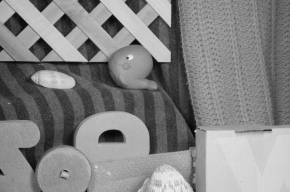
Figure 3: Decomposition of an image for four CPU.

Each CPU communicates the computed flow on the common boundary to his neighbor. So the more CPU we have, the more important the communication time is. More, the estimation of the optical flow is very sensitive at the boundary. For these reasons we want to optimize the number of pixels at the boundary of each part of the image. This is why we look for the largest ratio $\frac{\text{area}}{\text{perimeter}}$ where area is the total number of pixels in the sub-domain and perimeter is the number of pixels on the boundary. In the figure 4, we propose an example of a $48\times 48$ grid and a decomposition for twelve CPU. We give the different values of this ratio with respect to every possible splittings. Because the grid is squared in this example, the ratio is the same for the symmetric decompositions. Finally, we can see that the ratio is better if we split the image in $4\times 3$ (or $3\times 4$).

Figure 4: Evolution of the ratio on a $48\times 48$ grid and twelve CPU.

Since the optical flow estimation is sensitive at the boundaries, we use an additive Schwarz method to improve the estimation on the interfaces. This method requires an overlapping between the subdomains.

3.2 Model decomposition

We note $\Omega_{i}$ the part of the image corresponding to the $\text{CPU}_{i}$ and $\mathcal{J}_{i}$ the set of all indexes $j$ which are neighbors to $i$. We define $\Sigma_{i,j}=\Omega_{i}\cap\Omega_{j}$ and $\Gamma_{i,j}=\partial\Sigma_{i,j}\backslash\partial\Omega_{j}$ (See figure 5).

Figure 5: Example of notations for CPU $i=2$.

By using the additive Schwarz method to find an estimation $\textbf{U}_{i}$ of the optical flow in the part $\Omega_{i}$, the problem related to (8) is

$$-\text{div}(\Lambda^{k}\nabla\textbf{U}^{k}_{i})+A_{\rho}\textbf{U}^{k}_{i}=\textbf{F}\text{ in }\Omega_{i}$$

$$\frac{\partial\textbf{U}^{k}_{i}}{\partial n}=0\text{ on }\partial\Omega_{i}\backslash\Gamma_{i,j},\ \forall j\in\mathcal{J}_{i}$$ (14)

$$\textbf{U}^{k}_{i}=\textbf{U}^{k-1}_{j}\text{ on }\Gamma_{i,j},\ \forall j\in\mathcal{J}_{i}.$$

Thanks to this method the sequences $(\textbf{U}_{i}^{k})$ converge to $\textbf{U}_{|_{\Omega_{i}}}$. The rate of convergence increases with respect to the size of $\Sigma_{i,j}$. Another convergent method presented by P.-L. Lions [11] exists with the Robin boundaries conditions.

3.3 Multi-level parallel method

To solve the system with the finite element method we use the sofware FreeFem++ [9]. The default solver of this software for linear systems is UMFPACK (Unsymmetric MultiFrontal method) which allows to use non-symmetric matrices. The drawback of this library is that it can only solve problems smaller than 4GB. It means that we can’t treat parts larger than about $500\times 500$ pixels per CPU so we need to cut the whole image enough in the case of large images. This implies to have a large number of CPU which is not always the case depending on the machine we work with.

To overcome this issue, we use the MUMPS (MUltifrontal Massively Parallel sparse direct Solver) library which allows the resolution of sparse linear problems in parallel. The advantage of this solver is that it is not limited by the size of the problem, so we are able to use high definition sequences. It also ensures, to some extent, the scalability (see figure 13). However, it enforces to apply an LU decomposition to the matrix which can be long if this one is large (see figure 15). Combining the domain decomposition method with the use of the MUMPS library (see figure 6), we can reduce the computation time of the high definition sequence estimation.

Figure 6: Decomposition of an image for four groups of CPU.

The image is split in the same way as above according to the maximal ratio between the perimeter and the area of the part. The number of the group in which belongs the $\text{CPU}_{i}$ is given by

$$\text{group}(\text{CPU}_{i})=i\%(\text{nbPart})$$

where the binary operator $a\%b$ states for the remainder of the division of $a$ by $b$ and nbPart is the number of parts in the split image. The rest of the implementation is the same that the domain decomposition without MUMPS except that we act on a group instead of a single CPU.

4 Numerical Results

To test our algorithms, we use the RubberWhale sequence (figure 7) given by the Middleburry website at www.vision.middleburry.edu/flow/.

Figure 7: Frames 10 and 11 of the RubberWhale sequence.

Following their convention, we represent the estimated vector field thanks to a color map (figure 8) which assigns a color to each vector with respect to its orientation and its norm.

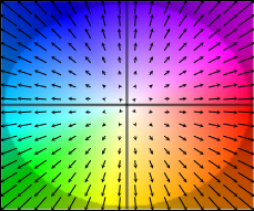
Figure 8: Vector field and its corresponding color map.

To validate our implementation, we compare our results with the exact solution also provided by Middelburry (figure 9).

Figure 9: Ground truth solution of the RubberWhale sequence.

For optical flow problems, the accuracy of the method is usually evaluated by computing the Average Angular Error (AAE) given by

$$AAE=acos\frac{u_{1,h}u_{1,e}+u_{2,h}u_{2,e}+1}{\sqrt{(u_{1,h}^{2}+u_{2,h}^{2}+1)(u_{1,e}^{2}+u_{2,e}^{2}+1)}}$$

and the Endpoint Error (EE) given by

$$EE=\sqrt{(u_{1,h}-u_{1,e})^{2}+(u_{2,h}-u_{2,e})^{2}}$$

where $\textbf{u}_{h}=(u_{1,h},u_{2,h})$ is an approximation of the vector field and $\textbf{u}_{e}=(u_{1,e},u_{2,e})$ represents the exact optical flow. Using the resolution of the system (7), our algorithm reaches an average angular error equals to 20.89 and an endpoint error equals to 0.38. In the litterature, the best angular errors go from 1 to 15 and the endpoint errors from 0.07 to 0.39 for the equivalent evaluation test case called Army (see the evaluation table at http://vision.middlebury.edu/flow/eval/results/results-a1.php). There are two reasons to explain that our error is large compared to these values. First, we recall that FreeFem++ [9] uses unstructured meshes and the computation of the angular error is not invariant with respect to the choice of the mesh. The other reason is that, even if we obtain a good approximation of the vector field direction (see the results presented bellow), due to the large value of the regularization in the non-egde areas, we under-estimate the vector norms. There exists some iterative strategy to improve this value but since we are principally interested in improving the computational time and in the adaptation of the regularization parameter, we don’t use it. To validate the domain decomposition, we need to verify the convergence of the Schwarz method which means that

$$\mid\textbf{U}^{k}-\textbf{U}^{k+1}\mid\underset{k\to\infty}{\longrightarrow}0.$$

We have split the image in four parts and tested the impact of the size of the overlap by using three different values, see figure 10.

Figure 10: Convergence of the Schwarz method for three different overlaps.

We can see that the Schwarz method has a fast convergence and that the speed of convergence increases with the size of the overlap. However, if the overlap is large, the time of the construction of the matrix $A$, which is the longest part of the code, is large too. Hence, we need to choose the size of the overlap considering an optimal ratio between the rate of convergence and the speed of computation time. Therefore, we choose an overlap of five pixels in the following tests.

Figure 11: Computation time with respect to the overlap.

There exist other methods without overlapping which may be theoretically faster [11]. In a forthcoming work, we will consider this class of methods. However, as we have seen, an overlap of 5 pixels is enough, so for large images the additional time can be neglected. On the figure 12, we present the evolution of the estimation according to the iterations of the Schwarz method. We can see that since the third iteration, we already have a good estimation of the solution at the interfaces.

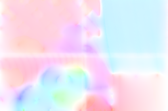
Figure 12: Results for a 2x2 separation, one image per iteration of Schwarz and with an overlap of five pixels.

In order to test the implementation of the multi-level parallelism, we have launched the same test case for different splittings of the image (2, 4 and 8 parts) and different numbers of CPU Per Part (CPP). In all cases, we have done ten iterations of the Schwarz method and we have kept an overlap of five pixels. On the figure 13, we present the improvement of the computation times.

Figure 13: Computation times of different configurations of the multi-level parallelism.

To understand the low efficiency of the multi-level implementation in the case where we use 32 CPU and split with 4 parts, we first represent on the figure 14 the communication times obtained in the different cases.

Figure 14: Communication times with respect to the number of CPU and the splitting (does not include the intern communications due to the MUMPS solver).

The increase of the communication times is not enough to explain the result obtained. Indeed, in every parallel implementations, the communication times increase with respect to the number of CPU used but it is usually balanced with the time saved in the computations. So, in order to give more details, we present in the figure 15 the times of the two main parts of the computation: the construction of the mass matrix and the LU factorization with the resolution part. We can see that adding more CPU to a part slightly increases the time of construction of the mass matrix. However, it allows to decrease the time of the LU factorization. On our architecture, if we split the images into several parts, the main part of the computation is the mass matrix construction. If we use a large number of CPU per part, we reduce the difference between the time saved in the LU decomposition and the time lost in the matrix construction. More, we increase the communication times and the MUMPS parallel solver doesn’t balance that.

Figure 15: Detailed computations times.

To evaluate the accuracy of the computed flow in the case of varying illumination, we use the RubberWhale test case where we have modified the first frame by increasing the brightness intensity (see figure 16). Since we haven’t modified the motion between the two pictures, the exact solution is the same that in the previous test case.

Figure 16: Modified first frame of the RubberWhale sequence for the varying illumination test case.

On the figure 17, we present the result obtained with and without the treatment of the brightness variation. On the right hand side, we can see that the solution without treatment is not well estimated. On the other hand, the model which uses the modified assumption (6) allowing the brightness variation gives a much accurate optical flow still well oriented.

Figure 17: Left: Estimation with (right) and without (left) treatment of the varying illumination. The images were split in four parts.

The next test (figure 18) consists of evaluating the efficiency of the adaptive regularization. The adaptation steps are done with the Schwartz iterations. We obtain a better definition of the edges.

Figure 18: Estimated optical flow after ten iterations of adaptation (result for a 2x2 separation).

On the figure 19, we can see that the adaptive regularization is still working for the test with non-constant brightness. In this case, the edges are even better defined.

Figure 19: Estimated optical flow after ten iterations of adaptation for the test with varying illumination (results for a 2x2 separation).

Finally, on the figures 20 and 21, we have used two sequences of real images provided by the Centre d’études et d’expertise sur les risques, l’environnement, la mobilité et l’aménagement (Cerema). These pictures present two main interests. First, the high resolution. We have $2028\times 1098$ pixels for the highway sequence and $1524\times 1092$ pixels for the wall sequence which corresponds to a vector field of about two billions of pixels to determine. The second interest is that the brightness and the texture are natural.

The highway sequence presents a non-constant brightness with a more complex texture and a lot of occlusions as the white lines on the road or the large motion of the car. We can see on the figure 20, the difference between the model with and without the varying illumination. On the left hand side, we have the solution without treatment. Again, we see that this is not correctly estimated because of the variation of the natural lighting. On the right, despite the occlusion areas which could be improved with a large displacement algorithm, we obtain a better approximation.

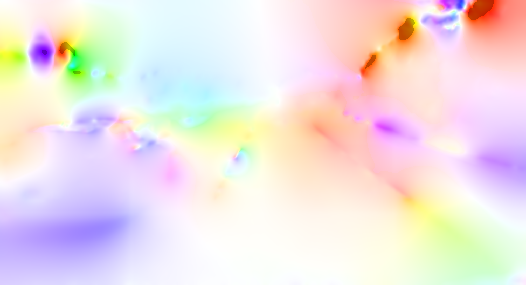
Figure 20: Up: Test case of the Highway sequence given by the Cerema. Bottom: Optical flow estimation obtained with (right) and without (left) treatment of the varying illumination. The images were divided in sixteen parts.

The figure 21 represents a wall of a tunnel. On this sequence the motion to estimate is linear. The challenge is to deal with irregular textures. This figure shows that our method is still efficient in this case. Indeed, the solution is quite smooth and linear except for the white square (bottom right) which may be improved by using a large displacement algorithm. This approach will be implemented in a further work.

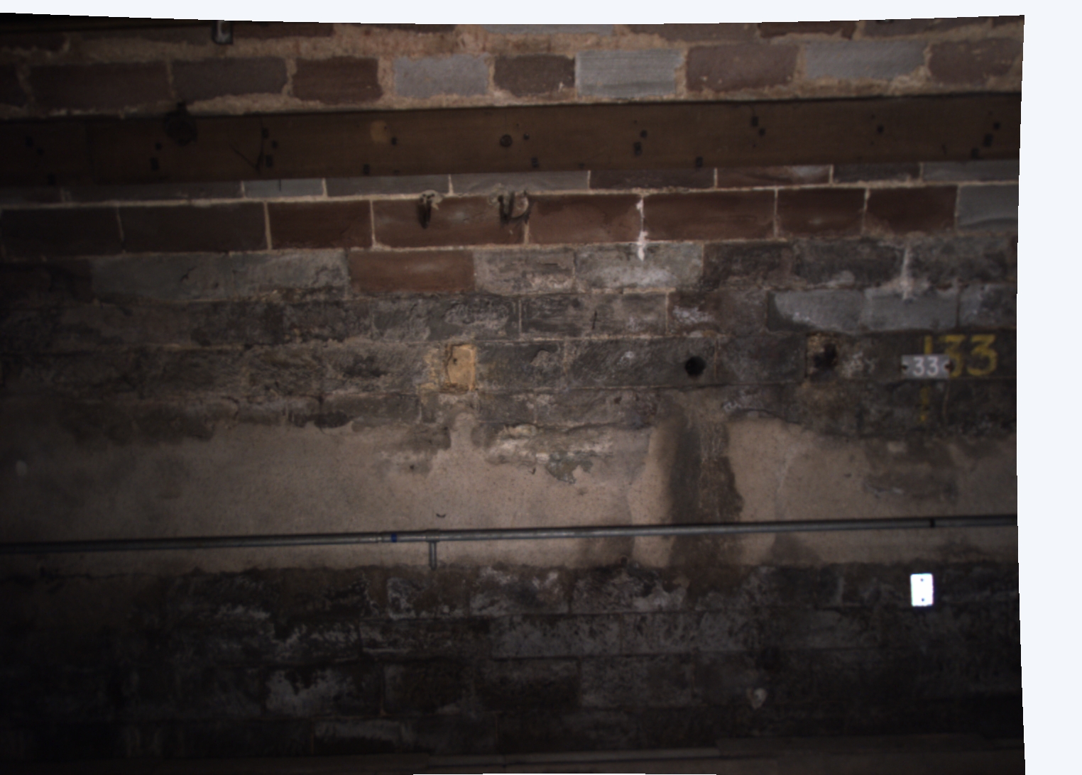
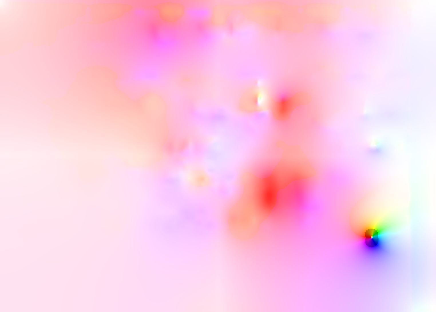
Figure 21: Up: Test case of the Wall sequence given by the Cerema. Bottom: Optical flow estimation obtained with (right) and without (left) treatment of the varying illumination. The images were divided in sixteen parts.

In the figure 22, we give the computation times obtained with the two high definition tests. We recall that the pictures have about two billions of pixels and were not reduced. As in the previous cases, we perform ten iterations of the Schwarz algorithm.

Figure 22: Computation times of the high definition tests for different splittings.

Conclusion

In this article we have used the finite element method to solve the optical flow problem with varying illumination. Thanks to the additive Schwarz method, we have implemented the domain decomposition in order to parallelize the computations. We have shown that this method is an efficient way to decrease the computation time and to handle high resolution sequences. We have also used a second level of parallelism in order to reduce the execution time even more and we have shown that such a massively parallel approach yields to an important gain of time.

The finite element method has also permitted to use an adaptive strategy of the regularization parameter, hence to efficiently combine the quality of the optical flow estimation with a method that preserves the edges and the fine features of the computed flow.

Acknowledgments: The authors would like to thank the Centre d’etudes et d’expertise sur les risques, l’environnement, la mobilité et l’aménagement (Direction territoriale Est, laboratoire de Strasbourg) for their suggestions and their data.

References

- [1] G. Aubert, R. Deriche, and P. Kornprobst. Computing optical flow via variational techniques. SIAM Journal on Applied Mathematics, 60(1):156–182, 1999.
- [2] J.L. Barron, D.J. Fleet, and S.S. Beauchemin. Performance of optical flow techniques. International Journal of Computer Vision, 12(1):43–77, 1994.
- [3] Z. Belhachmi and F. Hecht. An adaptive approach for segmentation and tv denoising in the optic flow estimation. to appear.
- [4] Z. Belhachmi and F. Hecht. Control of the effects of regularization on variational optic flow computations. Journal of Mathematical Imaging and Vision, 40(1):1–19, 2011.
- [5] T. Brox, A. Bruhn, N. Papenberg, and J. Weickert. High accuracy optical flow estimation based on a theory for warping. In Tomás Pajdla and Jiří Matas, editors, Computer Vision - ECCV 2004, volume 3024 of Lecture Notes in Computer Science, pages 25–36. Springer Berlin Heidelberg, 2004.
- [6] A. Bruhn. Variational optic flow computation: Accurate modelling and efficient numerics. PhD thesis, Université de Saarland, 2006.
- [7] A. Bruhn, J. Weickert, and C. Schnörr. Lucas/kanade meets horn/schunck: Combining local and global optic flow methods. International Journal of Computer Vision, 61(3):211–231, 2005.
- [8] M. Gennert and S. Negahdaripour. Relaxing the brightness constancy assumption in computing optical flow. 1987.
- [9] F. Hecht. New development in freefem++. J. Numer. Math., 20(3-4):251–265, 2012.
- [10] B. Horn and B. Schunck. Determining optical flow. Artificial Intelligence, 17(1):185 – 203, 1981.
- [11] P.-L. Lions. On the schwarz alterning method. iii: A variant for nonoverlapping subdomains. In Third internationnal symposium on domain decomposition methods for partial differential equations, volume 6, pages 202–223. SIAM Philadelphia, PA, 1990.
- [12] B. D. Lucas and T. Kanade. An iterative image registration technique with an application to stereo vision. In Proceedings of the 7th International Joint Conference on Artificial Intelligence - Volume 2, IJCAI’81, pages 674–679, San Francisco, CA, USA, 1981. Morgan Kaufmann Publishers Inc.
- [13] Y. Mileva, A. Bruhn, and J. Weickert. Illumination-robust variational optical flow with photometric invariants. In FredA. Hamprecht, Christoph Schnörr, and Bernd Jähne, editors, Pattern Recognition, volume 4713 of Lecture Notes in Computer Science, pages 152–162. Springer Berlin Heidelberg, 2007.
- [14] E. Mémin and P. Pérez. A multigrid approach to hierarchical motion estimation. In Proc. Int. Conf. on Computer Vision, ICCV’98, pages 933–938, Bombay, India, January 1998.
- [15] P. Ruhnau, T. Kohlberger, C. Schnörr, and H. Nobach. Variational optical flow estimation for particle image velocimetry. Experiments in Fluids, 38(1):21–32, 2005.
- [16] J. Weickert, A. Bruhn, N. Papenberg, and T. Brox. Variational optic flow computation: From continuous models to algorithms. In International Workshop on Computer Vision and Image Analysis (ed. L. Alvarez), IWCVIA’03, Las Palmas de Gran Canaria, 2003.
- [17] J. Weickert and C. Schnörr. Variational optic flow computation with a spatio-temporal smoothness constraint. Journal of Mathematical Imaging and Vision, 14(3):245–255, 2001.
- [18] H. Zimmer, A. Bruhn, J. Weickert, L. Valgaerts, A. Salgado, B. Rosenhahn, and H.-P. Seidel. Complementary optic flow. In Energy Minimization Methods in Computer Vision and Pattern Recognition, volume 5681, pages 207–220. Springer, 2009.