Asymmetric supernova remnants generated by Galactic, massive runaway stars

Abstract

After the death of a runaway massive star, its supernova shock wave interacts with the bow shocks produced by its defunct progenitor, and may lose energy, momentum, and its spherical symmetry before expanding into the local interstellar medium (ISM). We investigate whether the initial mass and space velocity of these progenitors can be associated with asymmetric supernova remnants. We run hydrodynamical models of supernovae exploding in the pre-shaped medium of moving Galactic core-collapse progenitors. We find that bow shocks that accumulate more than about $1.5\,\rm M_{\odot}$ generate asymmetric remnants. The shock wave first collides with these bow shocks $160-750\,\rm yr$ after the supernova, and the collision lasts until $830-4900\,\rm yr$. The shock wave is then located $1.35-5\,\rm pc$ from the center of the explosion, and it expands freely into the ISM, whereas in the opposite direction it is channelled into the region of undisturbed wind material. This applies to an initially $20\,\rm M_{\odot}$ progenitor moving with velocity $20\,\rm km\,\rm s^{-1}$ and to our initially $40\,\rm M_{\odot}$ progenitor. These remnants generate mixing of ISM gas, stellar wind and supernova ejecta that is particularly important upstream from the center of the explosion. Their lightcurves are dominated by emission from optically-thin cooling and by X-ray emission of the shocked ISM gas. We find that these remnants are likely to be observed in the [Oiii] $\lambda\,5007$ spectral line emission or in the soft energy-band of X-rays. Finally, we discuss our results in the context of observed Galactic supernova remnants such as 3C391 and the Cygnus Loop.

1 Introduction

Massive stars are rare but crucial to understand the cycle of matter in the interstellar medium (ISM) of galaxies (Langer, 2012). Significantly influenced by their rotation (Langer et al., 1999; van Marle et al., 2008; Chita et al., 2008), bulk motion (Brighenti & D’Ercole, 1995a, b) or by the presence of a companion (Stevens et al., 1992), their strong winds shape their surroundings and chemically augment their ambient medium (Vink, 2006). Some of these stars explode as luminous supernovae which release ejecta interacting with their pre-shaped environment (Borkowski et al., 1992; Vink et al., 1996, 1997; van Veelen et al., 2009). This event gives birth to supernova remnants replenishing the ISM with momentum and kinetic energy up to about $120\,\rm pc$ from the center of the explosion (Badenes et al., 2010).

Supernovae have been noticed in ancient Asia with the naked eye, e.g. the guest-star recorded in AD185 by chinese astronomers (Green & Stephenson, 2003), whereas the first supernova remnant has been identified spectroscopically almost two millennia later (Baade, 1938). Nowadays, surveys provide us with observations of Galactic supernova remnants, e.g. in gamma-rays (Abdo et al., 2010), X-ray (Pannuti et al., 2014), the infrared (Reach et al., 2006) or in submillimeter (van Dishoeck et al., 1993). Catalogues of remnants visible in the radio waveband in the northern and southern hemisphere are available in Kothes et al. (2006) and Whiteoak & Green (1996), respectively. An exhaustive catalogue of the known Galactic supernova remnants was compiled by Green (2009). These abundant observations reveal a diversity of complex morphologies such as shells, annuli, cylinders, rings and bipolar structures (cf. Gaensler, 1999).

The shape of young supernova remnants depends (i) on the geometry of the supernova explosion and (ii) on the (an)isotropy of their ambient medium (Vink, 2012). They therefore exhibit a wide range of morphologies that can be used to constrain their progenitors and/or ambient medium properties. The distribution of circumstellar matter depends on the progenitor properties (Bedogni & D’Ercole, 1988; Ciotti & D’Ercole, 1989; Dwarkadas, 2005, 2007) and the presence of ISM structures, e.g. borders of neighbouring diffuse nebulae or filaments that affect the propagation of the supernova ejecta. Models of remnants developing in a pre-existing wind cavity are shown in Tenorio-Tagle et al. (1990, 1991), and demonstrate that mixing of material happens in the former wind bubble. Multi-dimensional models of the formation of knots by wind-wind collision around Cassiopeia A are shown in Pérez-Rendón et al. (2009) and the effects of this fragmented Wolf-Rayet shell on the rebrightening of young remnants is explored in van Veelen et al. (2009). Supernova remnants developing through an edge of a dense region, e.g. a molecular cloud, give rise to champagne flows (Tenorio-Tagle et al., 1985). If the supernova happens near a denser region, the reverse shock is reflected towards the center of the explosion and a hot region of shocked material forms (Ferreira & de Jager, 2008). A strong magnetization of the ISM can induce a collimation of the supernova ejecta engendering elongated remnants (Rozyczka & Tenorio-Tagle, 1995).

Particularly, the bow shocks produced by runaway massive stars are an ideal site for the generation of an anisotropic circumstellar distribution. This is likely to happen in the Galactic plane, where most of the massive stars which are both in the field and classified as runaway are found (Gies, 1987; Blaauw, 1993; Huthoff & Kaper, 2002). A few of them are identified as evolved massive stars and three of them are red supergiants with detected bow shocks, i.e. Betelgeuse (Noriega-Crespo et al., 1997; Decin et al., 2012), $\mu$ Cep (Cox et al., 2012) and IRC$-$10414 (Gvaramadze et al., 2014). Consequently, and because these stars will explode as core-collapse supernova, their circumstellar medium is of prime interest in the study of aspherical supernova remnants.

The circumstellar medium of Galactic runaway red supergiant stars is numerically studied in Brighenti & D’Ercole (1995a, b) as an attempt to explain non-spherical supernova remnants. The works by van Marle et al. (2011) and Decin et al. (2012) tailor models to Betelgeuse’s bow shock and estimate in the context of recent observations (Cox et al., 2012) how the drag force on dust grains modifies the evolution of its contact discontinuity. The effects of the mass loss and space velocity on the shape and luminosity of bow shocks around red supergiant stars is investigated in Meyer et al. (2014, hereafter Paper  I). The repercussions of a weak ISM magnetic field on the damping of instabilities in the bow shocks of Betelgeuse is presented in van Marle et al. (2014). The stabilizing role of photoionization by an external source of radiation on the bow shock of IRC$-$10414 is shown in Meyer et al. (2014). The above cited models can be understood as investigations of the circumstellar medium of Galactic runaway core-collapse progenitors near their pre-supernova phase.

After the supernova explosion, the forward shock of the blastwave interacts with the free-streaming stellar wind (Chevalier & Liang, 1989; Chevalier, 1982). Supernovae showing evidence of interaction with circumstellar structures are commonly denoted as Type IIn and their corresponding lightcurves provide information on the progenitor and properties of its close surroundings (Schlegel, 1990; Filippenko, 1997; van Marle et al., 2010). About $10$$-$$100\,\rm yr$ after the explosion, the shock wave collides with the bow shock along the direction of motion of its progenitor, whereas it expands in a cavity of wind material in the opposite direction (Borkowski et al., 1992).

In this spirit, Rozyczka et al. (1993) model supernovae in oval bubbles generated by moving progenitors. They neglect the progenitor stellar evolution but demonstrate that elongated jet-like structures of size of about $10\,\rm pc$ form when the shock wave expands into the wind bubble. A model interpreting the cool jet-like [Oiii] $\lambda\,5007$ feature found in the Crab nebula (Blandford et al., 1983) as a shock wave channelled into the trail produced by its progenitor’s motion is presented in Cox et al. (1991).  Brighenti & D’Ercole (1994) show that if the runaway progenitor evolves beyond the main-sequence phase, the supernova explosion happens out of the main-sequence wind bubble, and the subsequent remnant develops as an outflow upstream from the direction of motion of the progenitor.

In this work, we aim to determine the degree of anisotropy of supernova remnants generated by runaway core-collapse progenitors moving through the Galactic plane. We model the circumstellar medium from near the pre-supernova phase of a representative sample of the most common runaway massive stars (Eldridge et al., 2011). We calculate one-dimensional hydrodynamic models of the supernova ejecta interacting with the stellar wind and use them as initial conditions for two-dimensional simulations of the supernova remnants. Finally, we discuss the emitting properties of the most aspherical of these remnants.

This project is different from previous studies (Brighenti & D’Ercole, 1994) because (i) we use self-consistent stellar evolution models, (ii) we consider both optically-thin cooling and heating along with thermal conduction, (iii) we trace the mixing between ISM, stellar wind and supernovae ejecta inside the remnants and (iv) our grid of models explores a broader space of parameters than works tailored to a particular supernova remnant, e.g. Kepler’s supernova remnant (Borkowski et al., 1992; Velázquez et al., 2006; Chiotellis et al., 2012; Toledo-Roy et al., 2014) or Tycho’s supernova remnant (Vigh et al., 2011). We neglect the magnetization, inhomogenity and turbulence of the ISM and ignore the cooling in the shock wave induced by the production of Galactic cosmic rays (Orlando et al., 2012; Schure & Bell, 2013). We assume that the supernova explosions do not have any intrinsic anisotropy. Furthermore, we assume than no pulsar wind nebula remains inside the supernova remnants and modifies the reflection of the reverse shock towards the center of the explosion (Bucciantini et al., 2003).

This paper is structured as follows. We begin Section 2 by discussing our numerical methods and initial parameters. The modelling of the circumstellar medium of our progenitors is shown in Section 3. We describe the calculations of supernova remnants developing inside and beyond their progenitors’ bow shock in Sections 4 and 5, respectively. Section 6 discusses and compares our models of aspherical remnants with observations. We conclude in Section 7.

2 Method and initial parameters

In this section, we review the numerical methods used to model the circumstellar medium of our progenitors and we present the procedure to set up supernova blastwaves.

2.1 Modelling the circumstellar medium

We perfom two-dimensional simulations using the code pluto (Mignone et al., 2007, 2012) to model the circumstellar medium of moving core-collapse supernova progenitors. We solve the equations of hydrodynamics in a cylindrical computational domain $(O;R,z)$ of origin $O$, which is coincident with the location of the runaway star and has rotational symmetry about $R=0$. A uniform grid of $N_{\rm R}\times N_{\rm z}$ grid cells is mapped onto a domain of size $[0,R_{\rm max}]\times[z_{\rm min},z_{\rm max}]$, respectively. We define $\mn@boldsymbol{\hat{R}}$ and $\mn@boldsymbol{\hat{z}}$ as the unit vectors of the axis $OR$ and $Oz$, respectively. The grid spatial resolution is $\mathit{\Delta}=R_{\rm max}/N_{\rm R}$. Following the method of Comerón & Kaper (1998), we release the stellar wind on a circle of radius $20$ grid cells centered on the origin and compute the wind-ISM interaction in the frame of reference of the moving progenitor.

We model the circumstellar medium of initially $10$, $20$ and $40\,\rm M_{\odot}$ stars moving with space velocity ranging from $v_{\star}=20$ to $70\,\rm km\,\rm s^{-1}$. The (time-dependent) stellar wind properties are taken from stellar evolution models (Brott et al., 2011). We consider a homogeneous ISM with a hydrogen number density $n_{\rm H}=0.57\,\rm cm^{-3}$ (Wolfire et al., 2003), i.e. we assume that the stars are exiled from their parent cluster and move in the low-density ISM. We set the ISM temperature to $T_{\rm ISM}\approx\,8000\,\rm K$ and include gain/losses by optically-thin radiative cooling assuming that the gas has solar metallicity (sections 2.3 and 2.4 of Paper I). All our bow shock models include electronic thermal conduction (Spitzer, 1962; Cowie & McKee, 1977).

We start our models at $t_{\rm start}\approx t_{\rm psn}-32\,t_{\rm cross}$, where $t_{\rm psn}$ is the time at the end of the stellar evolution model. The time interval $32\,t_{\rm cross}$ is sufficient to simulate these bow shocks getting rid of any switch-on effects arising during their development, where $t_{\rm cross}=R(0)/v_{\star}$ is the crossing-time and $R(0)$ is the stand-off distance of the bow shock (Baranov, Krasnobaev & Kulikovskii, 1971). The calculation of each bow shock model is followed until the end of the stellar evolution model, at $t_{\rm end}$. Note that our initially $10$ and $20\,\rm M_{\odot}$ progenitors explode as a red supergiant (Paper I). We run these models with the same underlying assumptions as in Paper I, especially considering that the stellar radiation field is not trapped by the bow shock (Weaver et al., 1977). Moreover, we assume that the evolutionary model of our initially $40\,M_{\odot}$ progenitor, that does not go all the way up to the pre-supernova phase, is sufficient to approximate the mass distribution at the time of the supernova explosion. Our stellar evolution models are described in section 2.2 of Paper I and the wind properties at $t_{\rm psn}$ are shown in Table 1.

Table 1: Wind properties at the end of the used stellar evolution models, at $t_{\rm psn}$. $M_{\star}\,(\rm M_{\odot})$ is the initial mass of each star, $\dot{M}\,(\rm M_{\odot}\,\rm yr^{-1})$ their mass loss and $v_{\rm wind}\,(\mathrm{km}\,\mathrm{s}^{-1})$ their wind velocity at a distance of $0.01\,\rm pc$ from the star, respectively. $T_{\rm eff}\,(\rm K)$ is the effective temperature of the stars (Brott et al., 2011).

$M_{\star}\,(\rm M_{\odot})$	$\dot{M}\,(\rm M_{\odot}\,\rm yr^{-1})$	$v_{\rm wind}\,(\mathrm{km}\,\mathrm{s}^{-1})$	$T_{\rm eff}\,(\rm K)$
$20$	$10^{-6.11}$	$16$	$3.2\times 10^{3}$
$40$	$10^{-4.79}$	$11$	$3.2\times 10^{3}$
$70$	$10^{-4.48}$	$50$	$5.8\times 10^{3}$

Our models of the circumstellar medium from near the pre-supernova phase are named with the prefix PSN followed by the initial mass of the progenitor $M_{\star}$ (first two digits, in $\mathrm{M}_{\odot}$) and its space velocity $v_{\star}$ (two last digits, in $\mathrm{km}\,\mathrm{s}^{-1}$). We adopt grid dimensions such that it includes the wake of the bow shocks produced during about $v_{\star}10t_{\rm cross}$ (our Table 2) in order to properly model the expansion of the shock wave through the tail of the bow shock up to times of the order of $10^{4}\,\rm yr$. The stellar wind is distinguished from the ISM material using a scalar $Q_{1}(\mn@boldsymbol{r})$ passively advected with the gas, where $\mn@boldsymbol{r}$ is the position vector of a grid cell. Its value is set to $Q_{1}(\mn@boldsymbol{r})=1$ for the wind material and to $Q_{1}(\mn@boldsymbol{r})=0$ for the ISM gas. Our cooling curves and numerical methods are extensively detailed in section 2 of Paper  I. Results are presented in Section 3.

Table 2: Input parameters used in our simulations of the bow shocks generated by supernova progenitors. Parameters $z_{\mathrm{min}}$ and $R_{\mathrm{max}}$ are the limits of the domain along the $x$-axis and $y$-axis (in $\mathrm{pc}$), respectively. $N_{\mathrm{R}}$ and $N_{\mathrm{z}}$ are the number of cells discretising the corresponding directions and $\it\Delta$ is the grid resolution (in $\mathrm{pc}\,\mathrm{{cell}^{-1}}$). The simulations start at a time $t_{\rm start}$ (in $\mathrm{Myr}$) after the star’s birth and are run until the end of the used stellar evolution models, at $\,t_{\rm psn}$ (in $\mathrm{Myr}$).

${\rm{Model}}$	$M_{\star}\,(\rm M_{\odot})$	$v_{\star}\,(\mathrm{km}\,\mathrm{s}^{-1})$	$z_{\mathrm{min}}\,(\mathrm{pc})$	$R_{\mathrm{max}}\,(\mathrm{pc})$	$N_{\rm R}$	$N_{\rm z}$	$\mathit{\Delta}\,(\mathrm{pc}\,\mathrm{cell}^{-1})$	$t_{\mathrm{start}}\,(\mathrm{Myr})$	$t_{\mathrm{psn}}\,(\mathrm{Myr})$
PSN1020	$10$	$20$	$-6.0$	$7.0$	$1225$	$1400$	$5.71\times 10^{-3}$	$23.7$	$24.7$
PSN1040	$10$	$40$	$-2.1$	$2.0$	$1143$	$1600$	$1.75\times 10^{-3}$	$24.5$	$24.7$
PSN1070	$10$	$70$	$-0.9$	$0.8$	$950$	$1425$	$8.42\times 10^{-4}$	$24.6$	$24.7$
PSN2020	$20$	$20$	$-30.0$	$35.0$	$2333$	$2333$	$1.49\times 10^{-2}$	$6.63$	$9.05$
PSN2040	$20$	$40$	$-9.0$	$8.0$	$600$	$1200$	$1.33\times 10^{-2}$	$8.65$	$9.05$
PSN2070	$20$	$70$	$-4.5$	$4.0$	$1067$	$1600$	$3.75\times 10^{-3}$	$8.70$	$9.05$
PSN4020	$40$	$20$	$-90.0$	$100.0$	$1500$	$1575$	$6.00\times 10^{-2}$	$0.0$	$4.5$
PSN4040	$40$	$40$	$-36.0$	$30.0$	$1500$	$2100$	$2.00\times 10^{-2}$	$2.00$	$4.5$
PSN4070	$40$	$70$	$-30.0$	$20.0$	$1000$	$2000$	$2.00\times 10^{-2}$	$3.50$	$4.5$

2.2 Setting up the supernova shock wave

We perform one-dimensional hydrodynamical simulations of the shock wave expanding into the stellar wind. The blastwave is characterized by its energy fixed to $E_{\rm ej}=10^{51}\,\rm erg$ and by the mass of the ejecta $M_{\rm ej}$. The latter is estimated as,

$$M_{\rm ej}=M_{\star}-\int_{t_{0}}^{t_{\rm psn}}\dot{M}(t)dt-M_{\rm co},$$ (1)

where $t_{0}$ and $t_{\rm psn}$ are the time at the beginning and the end of the used stellar evolution model, respectively. Note that we assume $M_{\rm ej}$ for our $40\,\rm M_{\odot}$ progenitor, because we ignore its post-main-sequence evolution. The quantity $M_{\rm co}=2\,\rm M_{\odot}$ in Eq. (1) is the assumed mass of the residual compact object left after the supernova (our Table 3).

Table 3: Simulations parameters used in our simulations of supernovae interacting with the unperturbed stellar wind. Parameter $M_{\rm ej}$ is the mass of the ejecta (in $\mathrm{M}_{\odot}$) and $r_{\mathrm{max}}$ is the size of the one-dimensional spherically symmetric domain (in $\rm pc$). The simulations are started at $t=0.04\,\mathrm{yr}$. The last column indicates the time at the end of our simulations, $t_{\mathrm{sncsm}}$ (in $\mathrm{yr}$).

${\rm{Model}}$	$M_{\mathrm{ej}}\,(\mathrm{M}_{\odot})$	$r_{\mathrm{max}}\,(\mathrm{pc})$	$t_{\mathrm{sncsm}}\,(\mathrm{yr})$
SNCSM 1020	$7.7$	$0.30$	$40$
SNCSM 1040	$7.7$	$0.20$	$13.5$
SNCSM 1070	$7.7$	$0.13$	$15$
SNCSM 2020	$17.7$	$0.90$	$40$
SNCSM 2040	$17.7$	$0.50$	$25$
SNCSM 2070	$17.7$	$0.25$	$20$
SNCSM 4020	$20$	$3.00$	$400$
SNCSM 4040	$20$	$1.50$	$200$
SNCSM 4070	$20$	$0.90$	$180$

We set up the supernova using the method detailed in Whalen et al. (2008) and in van Veelen et al. (2009). It assumes that the blastwave density profile $\rho(r)$ is a radial piece-wise function of the distance $r$ to the center of the explosion in the region $[0,r_{\rm max}]$, where $r_{\rm max}$ is the radius of the shock wave when we start the simulations. Under these assumption, the ejecta density profile is,

$$\rho(r)=\begin{cases}\rho_{\rm core}(r)&\text{if $r\leq r_{\rm core}$ },\\ \rho_{\rm max}(r)&\text{if $r_{\rm core}<r<r_{\rm max}$},\\ \rho_{\rm csm}(r)&\text{if $r\geq r_{\rm max}$},\\ \end{cases}$$ (2)

where,

$$\rho_{\rm core}(r)=\frac{1}{4\pi n}\frac{(10E_{\rm ej}^{n-5})^{-3/2}}{(3M_{\rm ej}^{n-3})^{-5/2}}t_{\rm max}^{-3},$$ (3)

is constant up to the inner core of radius $r_{\rm core}$ and,

$$\rho_{\rm max}(r)=\frac{1}{4\pi n}\frac{(10E_{\rm ej}^{n-5})^{(n-3)/2}}{(3M_{\rm ej}^{n-3})^{(n-5)/2}}\bigg{(}\frac{r}{t_{\rm max}}\bigg{)}^{-n},$$ (4)

is a steeply decreasing function of inner radius $r_{\rm core}$ and external radius $r_{\rm max}$ (Truelove & McKee, 1999). The power law index $n$ of Eq. (3)$-$(4) is set to the usual value $n=11$ for core-collapse supernovae (Chevalier, 1982). In relation (2), $\rho_{\rm cms}$ is the freely-expanding wind profile measured from the simulations along the symmetry axis $Oz$, in the direction of motion of the progenitor ($z\geq 0$). We use it as initial condition in the [$r_{\rm max}$,$r_{\rm sncsm}$] of the domain, where $r_{\rm sncsm}<R(0)$ is outer border of the domain.

The ejecta obey a homologous expansion, i.e. the velocity profile $v(r)$ is,

$$v(r)=\frac{r}{t},\,\mathrm{if}\,t>{\color[rgb]{0,0,0}t_{\rm max}},$$ (5)

where $t$ is the time after the supernova explosion. The ejecta velocity at $r_{\rm core}$ is therefore,

$$v_{\rm core}=\bigg{(}\frac{10(n-5)E_{\rm ej}}{3(n-3)M_{\rm ej}}\bigg{)}^{1/2},$$ (6)

(Truelove & McKee, 1999). The choice of $r_{\rm max}$ is free, as long as a mass of stellar wind smaller than $M_{\rm ej}$ is enclosed in $[r_{\rm max},r_{\rm sncsm}]$. We determined its $r_{\rm max}$ using the numerical procedure described in Whalen et al. (2008). We start the simulation at $t_{\rm max}=r_{\rm max}/v_{\rm max}$, where $v_{\rm max}$ is set to $30000\,\rm km\,\rm s^{-1}$ (van Veelen et al., 2009).

We choose a uniform grid of resolution $\Delta\leq 10^{-4}\,\rm{pc}\,\rm{cell}^{-1}$ and follow the expansion of the shock wave until slightly before it reaches the reverse shock of the bow shocks produced by our progenitors. These models are labelled with the prefix SNCSM (our Table 3). Additionally, we use a second passive scalar $Q_{2}(\mn@boldsymbol{r})$ to distinguish the ejecta from the stellar wind. We carry out these one-dimensional calculations using a uniform spherically symmetric grid. We use a finite volume method with the Harten-Lax-van Leer approximate Riemann solver, and integrate the Euler equations with a second order, unsplit, time-marching algorithm. Dissipative processes are computed using our cooling curve for fully ionized gas. Results are presented in Section 4.

2.3 Modelling the supernova remnants

In order to resolve both the early interaction between the blastwave interacting with the circumstellar medium and the old supernova remnant, we adopt a mapping strategy. We run two-dimensional hydrodynamical simulations of the shock waves interacting with the bow shocks using a squared computational domain of size about $4R(0)$ which is supplied with a uniform rectilinear grid. These models are labelled with the prefix YSNR. The above-described one-dimensional simulations of the ejecta interacting with the stellar wind are mapped into a circle of radius $r_{\rm max}<R(0)$ centered on the origin $O$ of the domain. We run these simulations starting at $t_{\rm sncsm}$ until the shock wave has passed through the forward shock of the bow shock and reaches a distance of about $2R(0)$ in the direction of motion of the progenitor, at $t_{\rm ysnr}$ (our Table 4).

The remnants at $t_{\rm ysnr}$ are mapped a second time onto a larger computational domain which includes both the entire pre-calculated circumstellar medium and the calculations of the young supernova remnants (our Tables 2 and 4). The regions of this domain which overlap neither the bow shock nor the remnant are filled with unperturbed ISM gas. We start the simulations at time $t_{\rm ysnr}$ and follow edge of the domain in the $-\mn@boldsymbol{\hat{z}}$ direction, at $t_{\rm osnr}$. These simulations are labelled with the prefix OSNR (our Table 5). Results are presented in Section 5.

Table 4: Input parameters used in our simulations of the supernova blastwaves interacting with the bow shocks of our progenitors. As input we use the solution of the shock waves interacting with the stellar winds (our Table 3). The grid parameters are similar as in our Table 2. Our simulations start at $t_{\mathrm{sncsm}}$ (our Table 2) shortly before that the shock wave interacts with the bow shock and the models are run until $t_{\mathrm{ysnr}}$ (in $\mathrm{yr})$ once the shock wave has gone through it.

${\rm{Model}}$	${\rm{Input}}$	$z_{\mathrm{min}}\,(\mathrm{pc})$	$R_{\mathrm{max}}\,(\mathrm{pc})$	$N_{\rm R}$	$N_{\rm z}$	$\it\Delta\,(\mathrm{pc}\,\mathrm{cell}^{-1})$	$t_{\mathrm{sncsm}}\,(\mathrm{yr})$	$t_{\mathrm{ysnr}}\,(\mathrm{yr})$
YSNR1020	SNCSM1020	$-2.0$	$2.0$	$1000$	$2000$	$2.0\times 10^{-3}$	$40$	$264$
YSNR1040	SNCSM1040	$-1.3$	$1.3$	$1000$	$2000$	$1.3\times 10^{-3}$	$13.5$	$150$
YSNR1070	SNCSM1070	$-0.7$	$0.7$	$1000$	$2000$	$4.0\times 10^{-4}$	$15$	$60$
YSNR2020	SNCSM2020	$-8.0$	$8.0$	$1000$	$2000$	$8.0\times 10^{-3}$	$40$	$2400$
YSNR2040	SNCSM2040	$-2.0$	$2.0$	$1000$	$2000$	$2.0\times 10^{-3}$	$20$	$450$
YSNR2070	SNCSM2070	$-1.0$	$1.0$	$1000$	$2000$	$1.0\times 10^{-3}$	$25$	$170$
YSNR4020	SNCSM4020	$-25$	$25$	$1000$	$2000$	$2.5\times 10^{-2}$	$400$	$4900$
YSNR4040	SNCSM4040	$-7.0$	$7.0$	$1500$	$3000$	$4.7\times 10^{-3}$	$200$	$1360$
YSNR4070	SNCSM4070	$-4.0$	$4.0$	$1500$	$3000$	$2.7\times 10^{-3}$	$180$	$830$

Table 5: Input parameters used in our simulations of the supernova blastwaves interacting with the tails of the bow shocks generated by our progenitors. As input we use the solution of the shock waves interacting with the bow shocks (our Table 4). The grid parameters are similar as in our Table 2. Our simulations start at $t_{\mathrm{ysnr}}$ (our Table 4) and the models are run until $t_{\mathrm{osnr}}$ (in $\mathrm{yr})$.

${\rm{Model}}$	${\rm{Input}}$	$z_{\mathrm{min}}\,(\mathrm{pc})$	$R_{\mathrm{max}}\,(\mathrm{pc})$	$N_{\rm R}$	$N_{\rm z}$	$\it\Delta\,(\mathrm{pc}\,\mathrm{cell}^{-1})$	$t_{\mathrm{ysnr}}\,(\mathrm{yr})$	$t_{\mathrm{osnr}}\,(\mathrm{yr})$
OSNR1020	YSNR1020	$-6.0$	$6.0$	$500$	$1000$	$1.2\times 10^{-2}$	$264$	$1500$
OSNR1040	YSNR1040	$-2.1$	$2.1$	$500$	$1000$	$4.2\times 10^{-3}$	$150$	$1300$
OSNR1070	YSNR1070	$-0.9$	$0.9$	$500$	$1000$	$4.0\times 10^{-4}$	$60$	$1300$
OSNR2020	YSNR2020	$-30.0$	$25.0$	$1000$	$2000$	$9.0\times 10^{-2}$	$2400$	$21100$
OSNR2040	YSNR2040	$-9.0$	$9.0$	$1000$	$2000$	$2.5\times 10^{-3}$	$450$	$15000$
OSNR2070	YSNR2070	$-4.5$	$4.5$	$1000$	$2000$	$9.0\times 10^{-3}$	$170$	$10000$
OSNR4020	YSNR4020	$-90.0$	$70.$	$1000$	$1714$	$7.0\times 10^{-2}$	$4900$	$49500$
OSNR4040	YSNR4040	$-35.0$	$25.0$	$1000$	$2200$	$2.5\times 10^{-2}$	$1360$	$14000$
OSNR4070	YSNR4070	$-30.0$	$15.0$	$700$	$2333$	$2.1\times 10^{-2}$	$830$	$10500$

3 The pre-supernova phase

In Fig. 1 we show the gas density fields in our bow shocks from near the pre-supernova phase in the models PSN1020 (initially $10\,\rm M_{\odot}$ star, $v_{\star}=20\,\rm km\,\rm s^{-1}$, Fig. 1a), PSN1040 (initially $10\,\rm M_{\odot}$ star, $v_{\star}=40\,\rm km\,\rm s^{-1}$, Fig. 1b) and PSN1070 (initially $10\,\rm M_{\odot}$ star, $v_{\star}=70\,\rm km\,\rm s^{-1}$, Fig. 1c). Figs. 2 and 3 show the same, but for our $20$ and $40\,M_{\odot}$ stars. The figures plot the density at a time $t_{\rm psn}$ and do not show all of the computational domain. In Figs. 1, 2 and 3 the overplotted solid black line is the contact discontinuity, i.e. the border between the wind and ISM gas where the value of the passive scalar $Q_{1}(\mn@boldsymbol{r})=1/2$.

The bow shocks of our $10$ and $20\,\rm M_{\odot}$ stars have morphologies consistent with previous studies (van Marle et al., 2011; Mohamed et al., 2012, Paper  I). Their overall shape is rather stable if $v_{\star}\leq v_{\rm w}$ (Dgani et al., 1996) and the flow inside the bow shocks is laminar (Fig. 1a). The bow shocks are unstable and exhibit Rayleigh-Taylor and/or Kelvin-Helmholtz instabilities for $v_{\star}\geq v_{\rm w}$ because of the large density difference between the dense red supergiant wind and the ISM gas (Figs. 1b,c and 2a,b). For high-mass stars moving with large space velocities, e.g. the models with $M_{\star}\geq 20\,\rm M_{\odot}$ and $v_{\star}\geq 40\,\rm km\,\rm s^{-1}$, the shocked layers develop non-linear thin-shell instabilities (Vishniac, 1994; Garcia-Segura et al., 1996; Blondin & Koerwer, 1998) and induce a strong mixing in the wakes of the bow shocks (Fig. 2c).

The stellar motion displaces the position of the star from the center of the cavity of unshocked wind material (Brighenti & D’Ercole, 1995a, b), and this displacement is larger for velocities $v_{\star}\geq 20\,\rm km\,\rm s^{-1}$ (Fig. 2a). The bow shocks which have the most pronounced tunnels of low-density gas are produced either by our initially $20\,\rm M_{\odot}$ star moving with $20\,\rm km\,\rm s^{-1}$ or by our initially $40\,\rm M_{\odot}$ star (Fig. 2a and 3a-c). In the region downstream from the progenitor, the reverse shock, which forms the walls of the cavity, has a rather smooth appearance for $v_{\star}\leq 20\,\rm km\,\rm s^{-1}$ (Fig. 2a) but it is ragged for $v_{\star}\geq 40\,\rm km\,\rm s^{-1}$ (Fig. 3c). Finally, note that the model PSN2020 has a double bow shock due to the final increase of the mass loss that ends the red supergiant phase. This structure is called a Napoleon’s hat and it develops when the bow shock from a new mass-loss event goes through the one generated by the previous evolutionary phase (Wang et al., 1993; Mackey et al., 2012).

The stand-off distance $R(0)$ and the mass $M$ trapped in the bow shocks upstream from the star ($z\geq 0$) are summarised in Table 6. The more massive bow shocks are the biggest ones, e.g. our bow shock model PSN4020 has the largest stand-off distance $R(0)\approx 5\,\rm pc$ and has accumulated about $116\,\rm M_{\odot}$ of shocked gas. They are generated by high-mass stars moving with small space velocities, i.e. $M_{\star}\geq 20\,\rm M_{\odot}$ and $v_{\star}\leq 40\,\rm km\,\rm s^{-1}$ (Figs. 2a-3ab). In Fig. 4 we show the average density profiles in our simulations of our $10$ (Fig. 4a), $20$ (Fig. 4b) and $40\,\rm M_{\odot}$ models (Fig. 4c), that we use as initial conditions for our one-dimensional simulations of the supernova shock waves interacting with their surroundings, see Eqs. (2)$-$(3). Fig. 4 illustrates that the most massive bow shocks have the largest $R(0)$, i.e. they are the most voluminous and are reached by the shock wave about $R(0)/v(r)\approx 10^{3}\rm yr$ after the explosion (Section 4).

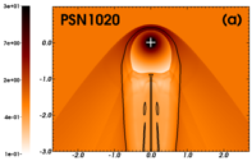
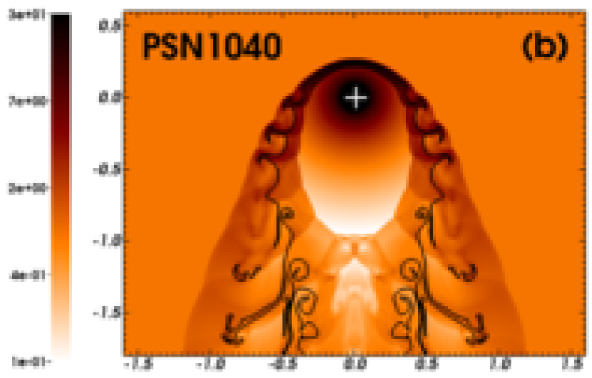
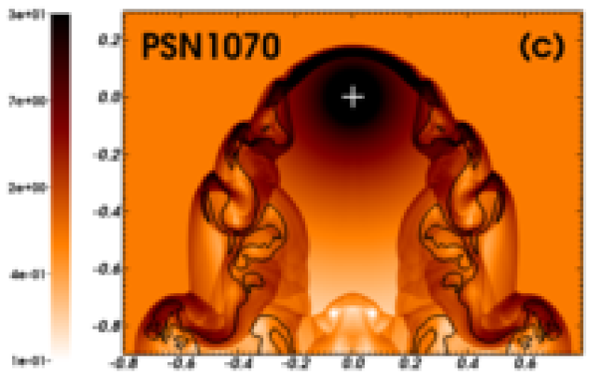
Figure 1: Grid of stellar wind bow shocks from the pre-supernova phase of our initially $10\,\rm M_{\odot}$ progenitor as a function of its space velocity with respect to the ISM, with velocity $v_{\star}=20$ (a), $40$ (b) and $70\,\mathrm{km}\,\mathrm{s}^{-1}$ (c). The nomenclature of the models follows Table 2. The bow shocks are shown at $t_{\rm psn}$. The gas number density is shown with a density range from $10^{-1}$ to $30.0\,\mathrm{cm}^{-3}$ in the logarithmic scale. The white cross marks the position of the star. The solid black contour traces the boundary between wind and ISM material $Q_{1}(\mn@boldsymbol{r})=1/2$. The $x$-axis represents the radial direction and the $y$-axis the direction of stellar motion (in $\mathrm{pc}$). Only part of the computational domain is shown in the figures.

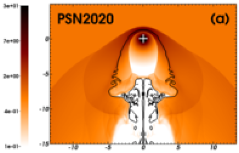
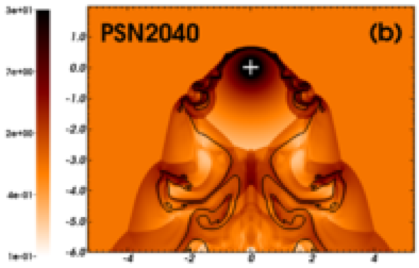
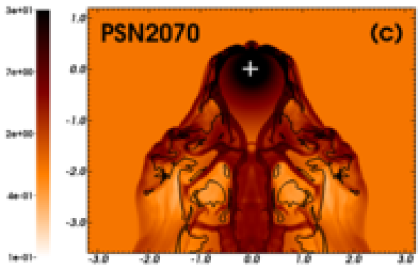
Figure 2: As Fig. 1, with our initially $20\,\rm M_{\odot}$ progenitor. Note the Napoleon’s hat structure of the bow shock in panel (a).

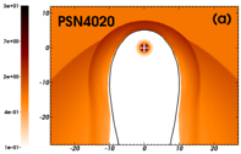
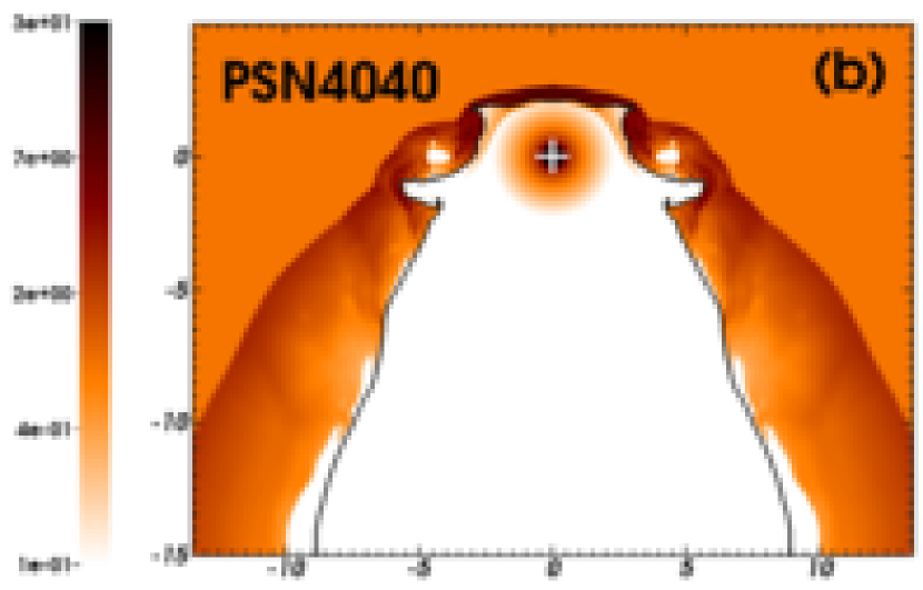
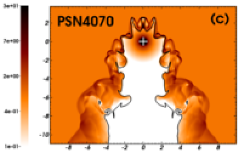
Figure 3: As Fig. 1, with our initially $40\,\rm M_{\odot}$ progenitor.

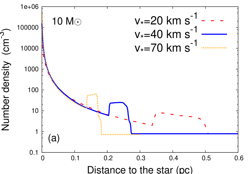
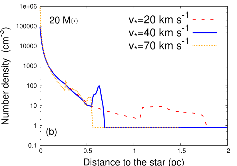
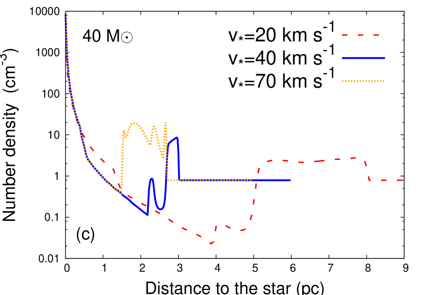
Figure 4: Gas number density profiles (in $\rm cm^{-3}$) taken along the direction of motion of our initially $10$ (a), $20$ (b) and $40\,\rm M_{\odot}$ (c) progenitors at $t_{\rm psn}$.

Table 6: Gas mass $M\,(\rm M_{\odot})$ in the region of the bow shocks that is upstream from the progenitor ($z\geq 0$) and stand-off distance at the contact discontinuity (in $\mathrm{pc}$) measured in our simulations of the circumstellar medium from near the pre-supernova phase, at a time $t_{\rm psn}$.

${\rm{Model}}$	$M\,(\rm M_{\odot})$	$R(0)\,(\rm pc)$
PSN1020	$0.06$	$0.42$
PSN1040	$0.03$	$0.25$
PSN1070	$0.01$	$0.17$
PSN2020	$3.87$	$1.35$
PSN2040	$1.10$	$0.64$
PSN2070	$0.75$	$0.55$
PSN4020	$116.00$	$5.00$
PSN4040	$9.40$	$2.70$
PSN4070	$1.65$	$1.55$

4 The young supernova remnant

This section presents our simulations of the supernova blastwaves interacting with their circumstellar medium until the shock wave reaches the outer layer of its surrounding bow shock. Spherical remnants are distinguished from asymmetric remnants as a function of their progenitors’ properties.

4.1 The ejecta-stellar-wind interaction

In Fig. 5 we show a typical interaction between a supernova shock wave and the surrounding stellar wind, before the shock wave collides with the bow shock. We plot the gas number density (solid blue line) and temperature (dashed red line) profiles in our model SNCSM1020 at a time about $22\,\rm yr$ after the supernova explosion. It assumes a release of $M_{\rm ej}=7.7\,M_{\odot}$ of ejecta together with a kinetic energy of $E_{\rm ej}=10^{51}\,\rm erg$ (our Table 3). The structure is composed of 4 distinct regions: the expanding ejecta profile, itself made of two regions, the core and the envelope (Truelove & McKee, 1999), the shell of swept up shocked ejecta and shocked wind material, and finally the undisturbed circumstellar material (Chevalier, 1982).

The shell is bordered by two shocks, a reverse shock that is the interface between ejecta and shocked ejecta, and a forward shock constituting the border between shocked wind and undisturbed freely-expanding stellar wind (Chiotellis et al., 2012). The core of the ejecta ($r<0.08\,\rm pc$) has a very low temperature because its thermal pressure is initially null (Whalen et al., 2008; van Veelen et al., 2009). The temperature slightly increases up to a few tens of degrees in the envelope of ejecta ($0.08\leq r\leq 0.16\,\rm pc$) because (i) we use a homologous velocity profile which results in increasing the thermal pressure close to the high-velocity shock wave and (ii) the decreasing density $\rho_{\rm max}\propto r^{-11}$ increases the temperature $T\propto p/\rho$. At radii $r\approx 0.16\,\rm pc$ is the hot ($T\approx 10^{6}\,\rm K$) and dense ($n\gg 10^{3}\,\rm cm^{-3}$) gas. This region between the shell and the shock wave is hot because it is shock-heated by the blastwave and it has not yet cooled. All our models have a similar behaviour.

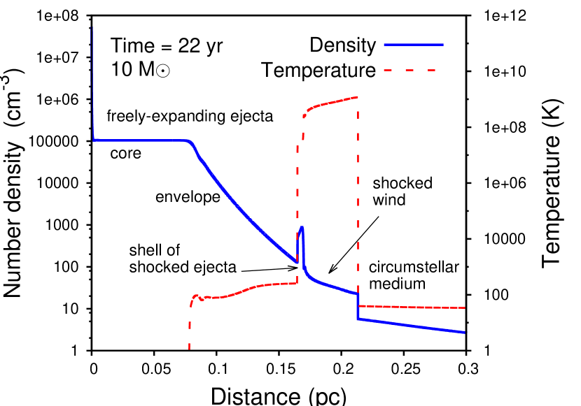
Figure 5: Total number density (solid blue line, in $\rm cm^{-3}$) and temperature (dashed red line, in $\rm km\,\rm s^{-1}$) profiles of the supernova ejecta interacting with the circumstellar medium of our initially $10\,\rm M_{\odot}$ progenitor. Profiles are shown at about $22\,\rm yr$ after the supernova explosion. The distinct regions composing the supernova remnant are indicated on the figure. The substructure of the shocked ejecta follows the nomenclature in Truelove & McKee (1999).

4.2 The shock wave interacting with the bow shock

The supernova interacting with the bow shock generated by the $10\,\rm M_{\odot}$ star moving with $v_{\star}=40\,\rm km\,\rm s^{-1}$ is illustrated in Fig. 6. We show the density field in our simulation YSNR1040, composed of a shock wave interacting with its circumstellar medium (our model SNCSM1040). The density stratification is shown at times $t_{\rm sncsm}\approx 152\,\rm yr$ (Fig. 6a), $154$, $162$, $168$, $192$ and $t_{\rm ysnr}\approx 246\,\rm yr$ (Fig. 6f) after the explosion, respectively. Note that the part of the computational domain plotted in Fig. 6f is larger than in Figs. 6a-e. Corresponding cross-sections measured in these density fields along the $Oz$ axis are shown in Fig. 7.

At a time $t_{\rm sncsm}\approx 152\,\rm yr$ the solution SNCSM1040 is mapped on the model PSN1040 shortly before the supernova remnant shock wave reaches the reverse shock of the bow shock (Fig. 6a). The organisation of the remnant is similar to the situation depicted in fig. 5 of Velázquez et al. (2006). From the origin to larger radius, the curve (a) of Fig. 7 plots the initial plateau of density $\rho_{\rm core}(r)\approx 10^{5}\rm cm^{-3}$, the steep profile $\rho_{\rm max}(r)\propto r^{-n}$, the shell of swept-up ejecta at about $0.16\,\rm pc$ (cf. Fig. 5), the shock wave progressing in the freely-expanding wind, the red-supergiant bow shock from about $0.21$ to about $0.27\,\rm pc$, and the unperturbed ISM.

In Fig. 6b the shock wave collides with the reverse shock of the bow shock and begins to interact with the dense ($n\approx\,25\rm cm^{-3}$) shocked wind. The interaction starts at the stagnation point because this is the part of the bow shock with the smallest radius (Borkowski et al., 1992). The blastwave decelerates and loses its spherical symmetry, the shock wave penetrates the reverse shock of the bow shock at a time $154\,\rm yr$ with velocity $v\approx 6700\,\rm km\,\rm s^{-1}$ whereas it hits its forward shock $8\,\rm yr$ later with velocity $v\approx 4500\,\rm km\,\rm s^{-1}$. At $162\,\rm yr$, the shell of shocked ejecta merges with the former post-shock region at the reverse shock of the bow shock, and its material is compressed to $n\approx\,85\,\rm cm^{-3}$ (curve (c) of Fig. 7).

In Fig. 6c the shock wave has totally penetrated the bow shock, both a reflected and a transmitted shock wave form at both the ends of the bow shock. In Fig. 6d the transmitted shock at the former forward shock starts expanding into the undisturbed ISM. As sketched in fig. 3 of Borkowski et al. (1992), a bump emerges beyond the bow shock and it reaches about $0.32\,\rm pc$ at a time $168\,\rm yr$ after the explosion (curve (d) of Fig. 7). It expands and enlarges laterally as the shock wave, that is no longer restrained by the material of the bow shock, penetrates the undisturbed ISM, accelerates and progressively recovers its spherical symmetry (Fig. 6e, see also Fig. 1 of Brighenti & D’Ercole, 1994).

At a time $246\,\rm yr$, the shock wave has recovered its sphericity (Fig. 6f). Note that the shock wave is slightly constricted in the cavity of unshocked wind as it expands downstream from the direction of motion of the progenitor. This anisotropy is a function of the circumstellar density distribution at the pre-supernova phase and governs the long term evolution of the supernova remnant (Section 4.3). The curve (f) of Fig. 7 shows the density structure composed of the plateau whose density has diminished to $\rho_{\rm core}\approx 600\,\rm cm^{-3}$, the twice shocked ejecta, the twice shocked stellar wind, twice shocked ISM, shocked ISM and finally the unperturbed ISM (c.f. Borkowski et al., 1992). These regions are not clearly discernible because of the mixing at work provoked by the multiple reflections and refractions proliferating through the remnant (curve (f) of Fig. 7). We underline that our one-dimensional, spherically-symmetric calculations do not allow us to model the Rayleigh-Taylor instabilities triggered at the interface between supernova ejecta and uniformly-expanding stellar wind (Chevalier et al., 1992). These instabilities may affect the propagation of the shock wave through the bow shock.

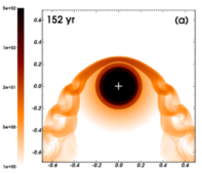
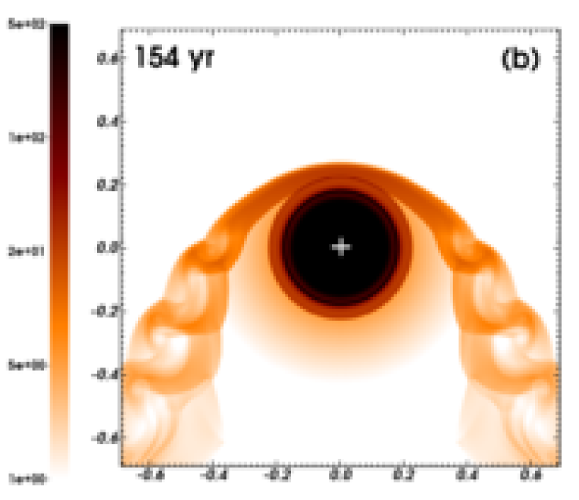
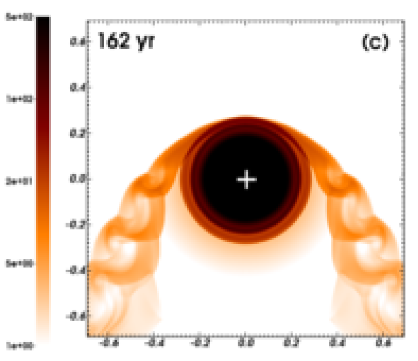
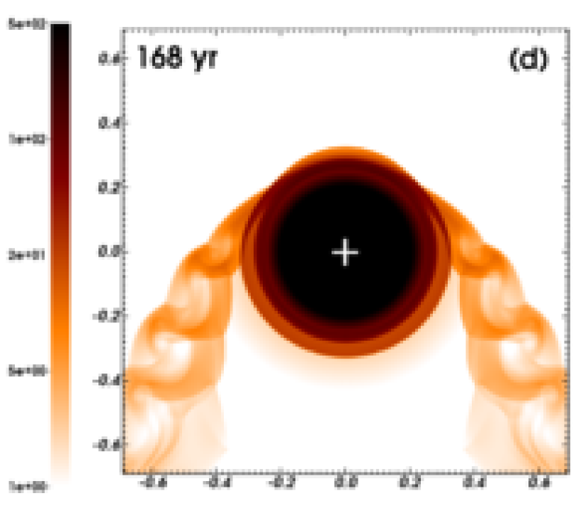
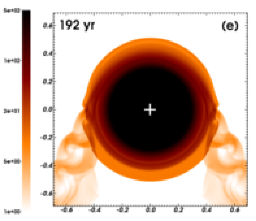
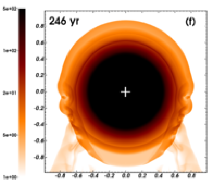
Figure 6: Time sequence of a supernova interacting with the bow shock generated by our initially $10\,\rm M_{\odot}$ progenitor moving with velocity $40\,\rm km\,\rm s^{-1}$. The figures correspond to times $t_{\rm sncsm}$ (a) up to about $t_{\rm ysnr}$ (f). The gas number density is shown with a density range from $1.0$ to $5\times 10^{2}\,\mathrm{cm}^{-3}$ on a logarithmic scale. The white cross marks the center of the explosion. The $x$-axis represents the radial direction and the $y$-axis the direction of stellar motion (in $\mathrm{pc}$). Only part of the computational domain is shown in the figures. Note that the panel (f) shows the supernova remnant at larger scale than in panels (a-e).

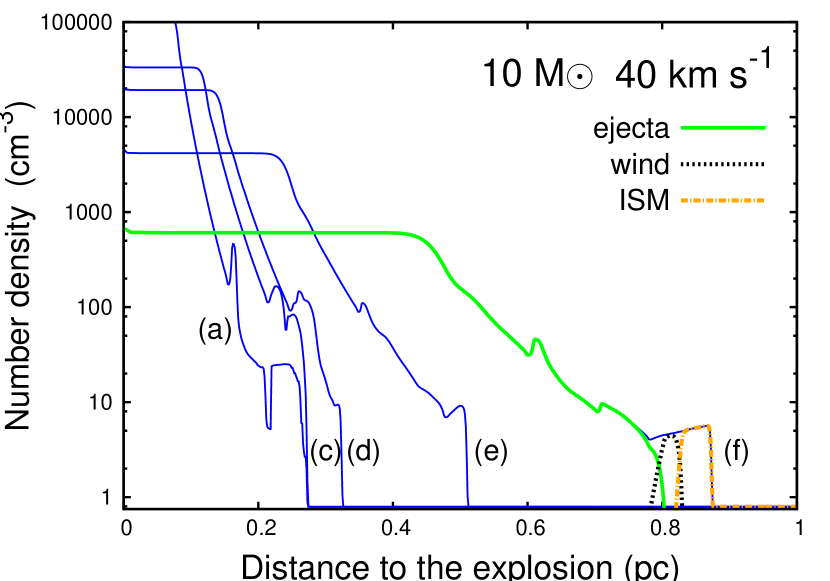
Figure 7: Cross-sections taken along the direction of motion of the progenitor through the number density field of the supernova blastwave interacting with the $z\geq 0$ region of the bow shock produced by our initially $10\,\rm M_{\odot}$ progenitor moving with velocity $40\,\rm km\,\rm s^{-1}$ (Fig. 6a-f). Note that the cross-section from Fig. 6b is omitted in the figure because it is very similar the curve (a). The respective proportion of the supernova ejecta (solid green), stellar wind (dotted black) and ISM material (dashed orange) are indicated for the curve (f).

4.3 Spherical and aspherical supernova remnants

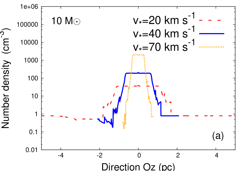
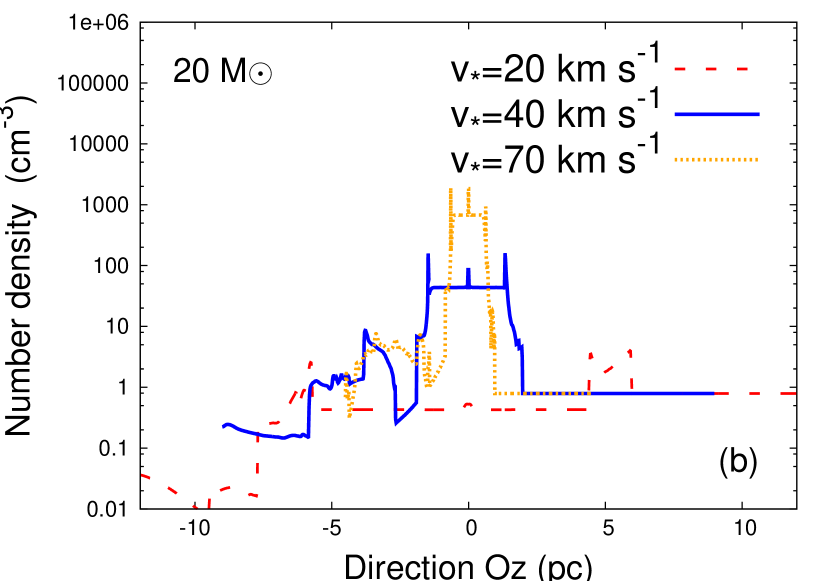
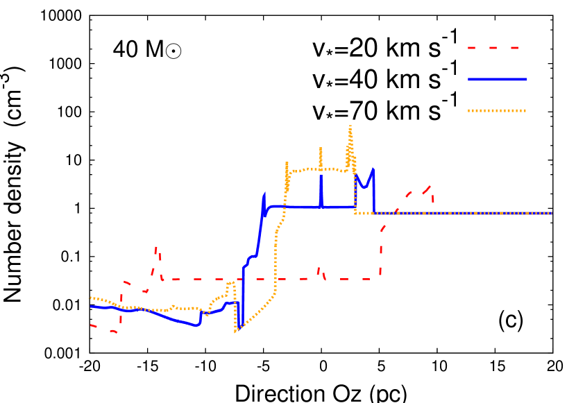
Figure 8: Density profiles (in $\rm cm^{-3}$) of our supernova remnants taken along the direction of motion of our initially $10$ (a), $20$ (b) and $40\,\rm M_{\odot}$ (c) progenitors, taken when the supernova shock wave has reached a distance of about $2R(0)$ in the direction of motion of the progenitors, at $t_{\rm ysnr}$.

In Fig. 8 we represent the density profiles of our models of supernova remnants at a time $t_{\rm ysnr}$, taken along the direction of motion of the progenitors. The models produced by our $10\,M_{\odot}$ progenitor conserve their symmetry after the shock waves collide with the bow shocks, e.g. our model YSNR1020 has a plateau of density $n\approx 10^{2}\,\rm cm^{-3}$ at $|z|\leq\,1.7\,\rm pc$, whereas its density distribution in both directions beyond the shock wave is about the ISM ambient medium density. Here, the shock wave expansion is barely disturbed by the light bow shocks (our Table 6) and the remnants grow quasi-spherically (Fig. 6).

The remnant generated by our $20\,\rm M_{\odot}$ star moving with $v_{\star}=20\,\rm km\,\rm s^{-1}$ is aspherical, in that it has a cavity of $n\approx 10^{-2}\,\rm cm^{-3}$ at $z<-8\,\rm pc$ (red curve in Fig. 8b). This is much less pronounced for models with a larger $v_{\star}$, i.e. our models YSNR2040 and YSNR2070, see blue and yellow curves in Fig. 8b. They have a rather spherical density distribution, and only a bulge of swept-up wind material in the direction $+\mn@boldsymbol{\hat{z}}$ distinguishes them from a spherically symmetric structure. A small accumulation of swept-up gas that could slightly decelerate the shock wave forms in the direction $-\mn@boldsymbol{\hat{z}}$, i.e., these models do form a pronounced wind cavity (Fig. 8bc).

The supernova remnants of our $40\,\rm M_{\odot}$ progenitor are all strongly anisotropic, e.g. our model with velocity $v_{\star}=70\,\rm km\,\rm s^{-1}$ has a dense shell of density $n\approx 10^{2}\,\rm cm^{-3}$ along the direction $+\mn@boldsymbol{\hat{z}}$ and a cavity of density $n\approx 10^{-2}\,\rm cm^{-3}$ in the opposite direction (Fig. 8c). On the basis of Table 6 and according to the above discussion, we find that the bow shocks of runaway stars that we simulate and which accumulate more than about $1.5\,\rm M_{\odot}$ generate asymmetric supernova remnants. We measure from our simulations that the collision between the shock waves and these dense bow shocks, located at $R(0)\approx\,1.35-5\,\rm pc$ from the center of the explosion, begins about $160-750\,\rm yr$ and ends about $830-4900\,\rm yr$ after the supernova, respectively. In the next section, we continue our study focusing on the asymmetric models only, i.e. generated either by our $20\,\rm M_{\odot}$ progenitor moving with $v_{\star}=20\,\rm km\,\rm s^{-1}$ or produced by our $40\,\rm M_{\odot}$ star.

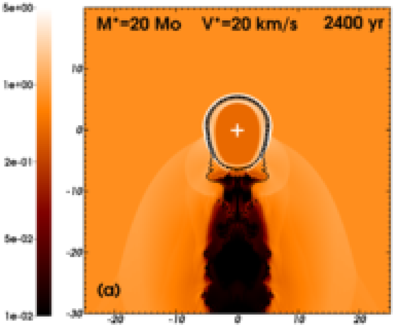
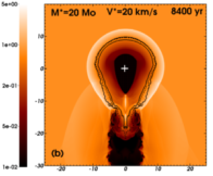
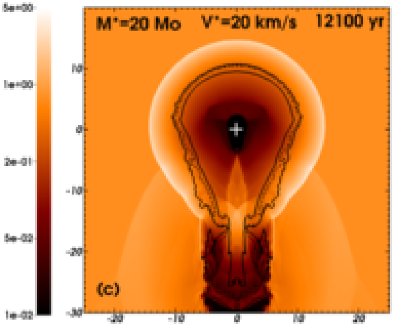
Figure 9: Time sequence of the evolution of the supernova remnant generated by our initially $20\,\rm M_{\odot}$ progenitor moving with velocity $20\,\rm km\,\rm s^{-1}$. The figures are shown at a time $t_{\rm ysnr}$ (a), at an intermediate time (b) and at the end of the simulation, at a time $t_{\rm osnr}$ (c). The gas number density is shown with a density range from $10^{-2}$ to $5.0\,\mathrm{cm}^{-3}$ on the logarithmic scale. The color scale is reversed compare to Fig. 1 to 3. The cross marks the center of the explosion. Note the Napoleon’s hat structure of the unperturbed circumstellar medium in panel (a). The solid black contours trace the boundary between stellar wind material and either the supernova ejecta or ISM gas $Q_{1}(\mn@boldsymbol{r})=1/2$. The dotted black contour is the discontinuity between supernova ejecta and wind material $Q_{2}(\mn@boldsymbol{r})=1/2$. The nomenclature of the models follows our Table 5. The $x$-axis represents the radial direction and the $y$-axis the direction of stellar motion (in $\mathrm{pc}$). Only part of the computational domain is shown in the figures.

5 The old supernova remnant phase

In this section we detail the interaction between supernova ejecta and pre-shaped circumstellar medium once the expanding front has passed through the bow shock. We focus on our four models of supernova remnants whose solutions strongly deviate from sphericity.

5.1 Physical characteristics of the remnants

5.1.1 Asymmetric structures…

We show the gas density fields in the old supernova remnant produced by our $20\,\rm M_{\odot}$ progenitor moving with velocity $v_{\star}=20\,\rm km\,\rm s^{-1}$ in Fig. 17. Figs. 10, 11 and 12 are similar, but showing our $40\,\rm M_{\odot}$ progenitor moving with velocity $v_{\star}=20$, $40$ and $v_{\star}=70\,\rm km\,\rm s^{-1}$, respectively. In each of these figures, panel (a) corresponds to a time $t_{\rm ysnr}$ (our Table 4), panel (b) shows the shock wave expanding into the wind cavity and panel (c) shows the remnant at $t_{\rm osnr}$ when the simulation ends (our Table 5). The figures do not show the full computational domain. In Figs. 17 to 12, the overplotted solid black line is the border between the wind and ISM gas where the value of the passive scalar $Q_{1}(\mn@boldsymbol{r})=1/2$, and the dashed black line is the discontinuity between the ejecta and the other materials where $Q_{2}(\mn@boldsymbol{r})=1/2$.

At a time $t_{\rm ysnr}$, the shock wave is already asymmetric because its unusually dense surroundings (see our Table 6) strongly restrain it from expanding into the direction normal to the direction of motion of the progenitor (panels (a) of Figs. 17 to 12). As an example, the forward shock in our model OSNR2020 at a time $2400\,\rm yr$ has reached about $5.8\,\rm pc$ and $6\,\rm pc$ along the $+\mn@boldsymbol{\hat{R}}$ and $+\mn@boldsymbol{\hat{z}}$ directions, respectively, whereas it expands to about $-7.9\,\rm pc$ along the $-\mn@boldsymbol{\hat{z}}$ direction. This asymmetry of the shock wave is particularly pronounced in our simulation OSNR4020 whose pre-shaped circumstellar medium contains the most massive bow shock with a mass of $116\,\rm M_{\odot}$ (Fig. 10ab).

At times larger than $t_{\rm ysnr}$, the shock wave freely expands into the undisturbed ISM in the $+\mn@boldsymbol{\hat{R}}$ and $+\mn@boldsymbol{\hat{z}}$ directions because it has entirely overtaken its circumstellar structure (Brighenti & D’Ercole, 1994), see Figs. 10-12bc. It progressively recovers its sphericity, but this takes longer in our simulations with slowly moving progenitors because the mass in their bow shock is larger (Fig. 10c and 12c). The penetration of the shock wave through the wake of the bow shock results in its chanelling into the tubular cavity of unshocked stellar wind (Blandford et al., 1983). The constant cross-sectional area of the cavity continues to impose large temperature and pressure jumps at the post-shock region of the shock wave, which prevents it from decelerating and which collimates the ejecta as a tubular/jet-like extension to the spherical region of shocked ejecta (Cox et al., 1991).

5.1.2 … of angle-dependent physical properties

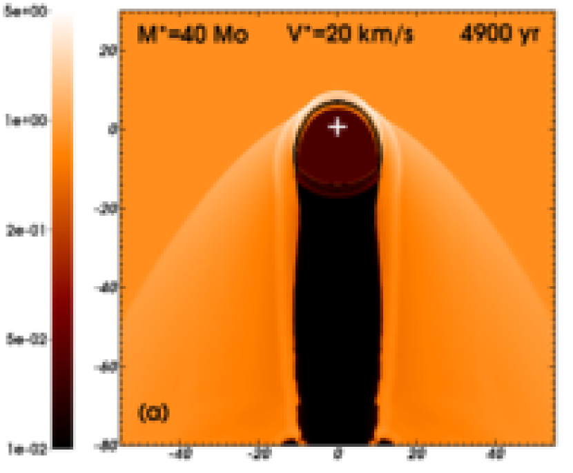
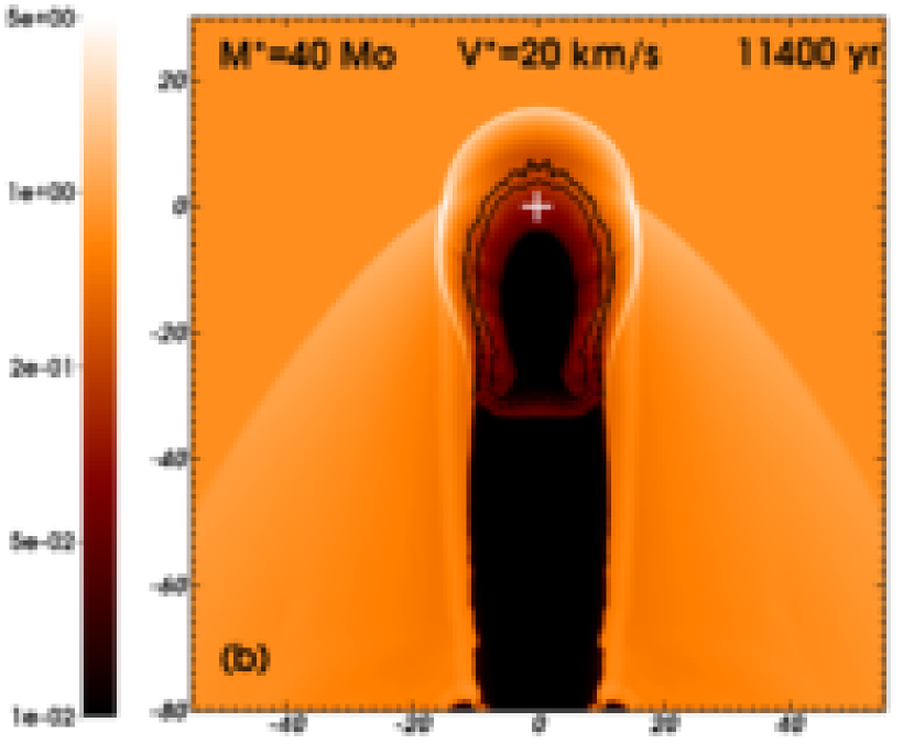
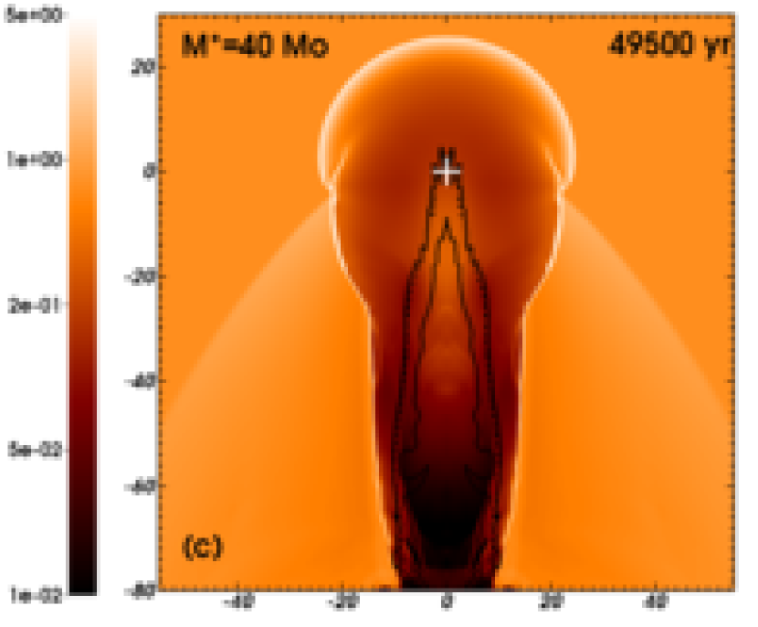
Figure 10: As Fig. 17, with our initially $40\,\rm M_{\odot}$ progenitor.

Fig. 13 plots the spatio-temporal evolution of the shock front measured in our apsherical remnants along the $+\mn@boldsymbol{\hat{z}}$ and $-\mn@boldsymbol{\hat{z}}$ directions. The shock wave typically expands into the ISM at velocities of the order of a few hundred $\rm km\,\rm s^{-1}$ whereas it propagates inside the trail of the bow shock with a velocity of the order of a few thousands $\rm km\,\rm s^{-1}$. E.g. at a time $4500\,\rm yr$ after the explosion, the model OSNR2020 has a shock wave velocity of $564$ and $1578\,\rm km\,\rm s^{-1}$ at $8.73$ and $13.03\,\rm pc$ from the center of the explosion in the direction along and opposite of the progenitor’s motion, respectively. The deceleration of the shock wave is more important for our slowly moving progenitors which induce the strongest anisotropy in their circumstellar medium (Fig. 13a-b), whereas the ejecta velocity is larger after the collision with the lighter bow shocks of our fast-moving progenitors (Fig. 13d and our Tab. 6).

Because the blastwave expand in non-uniform medium (Ferreira & de Jager, 2008), a wave created during the collision with the dense bow shock is reflected towards the center of the explosion and shocks back the unperturbed supernova ejecta (see Fig 17a-c). This mechanism generates a hot region of ejecta which progressively fills the entire cavity of the remnants, e.g. the shocked ejecta of our model OSNR2020 has $n\approx 3\,\rm cm^{-3}$ and $T\approx 10^{6}\,\rm K$ (Fig. 17bc). Simultaneously, the collimated shock wave continues expanding downstream from the center of the explosion. It hits the tunnel’s side, i.e., the walls of the wind cavity, which post-shock density increases up to about $30\,\rm cm^{-3}$ in model OSNR4020 and cools to less than $10^{5}\,\rm K$. The shocked walls produce strong optical line emission (Cox et al., 1991, see also Section 5.3).

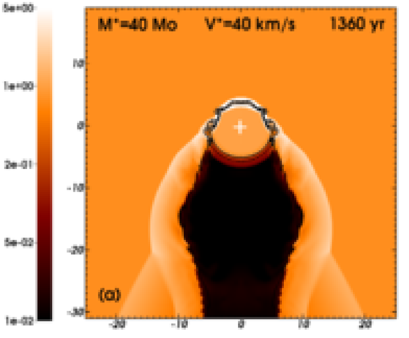
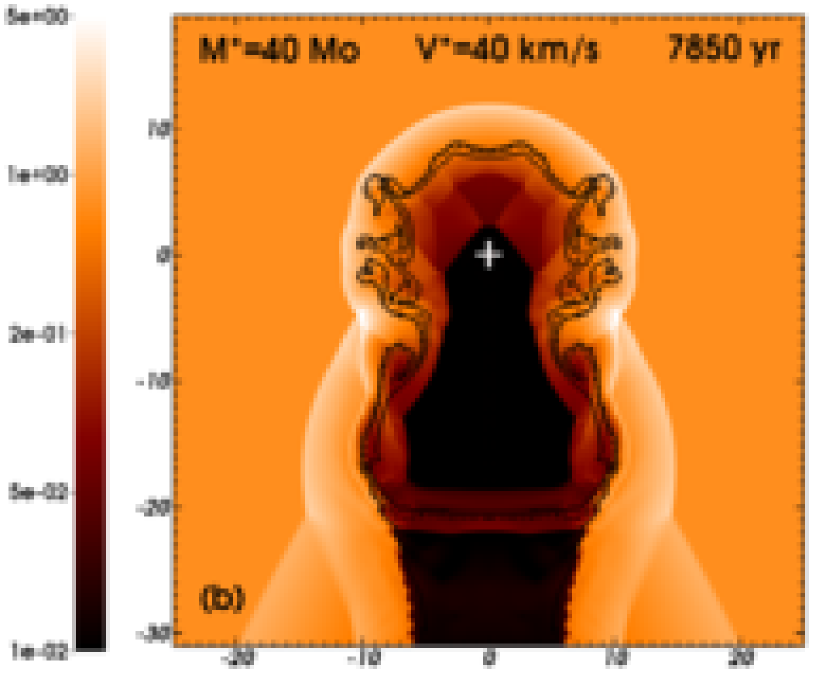
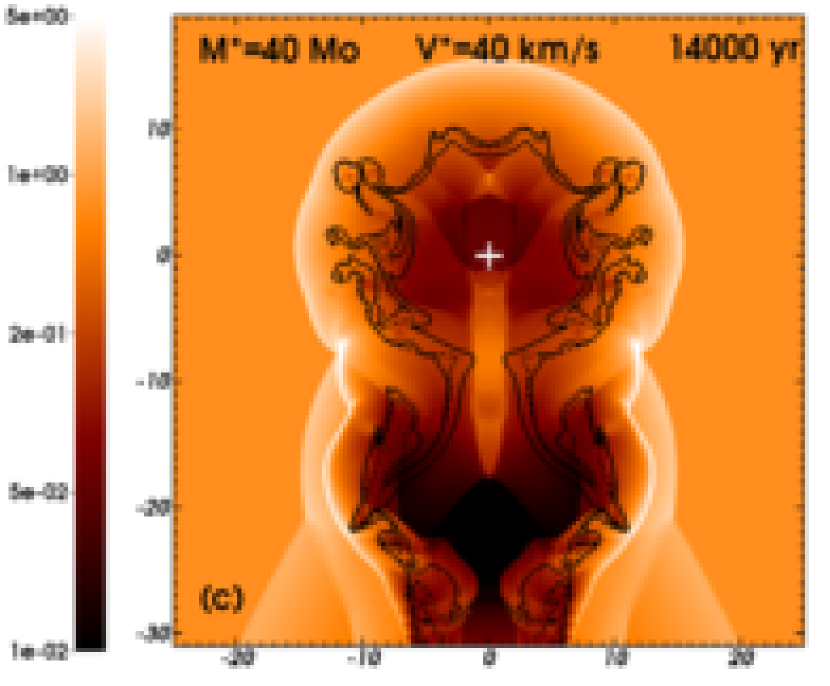
Figure 11: As Fig. 10, with space velocity $v_{\star}=40\,\rm km\,\rm s^{-1}$.

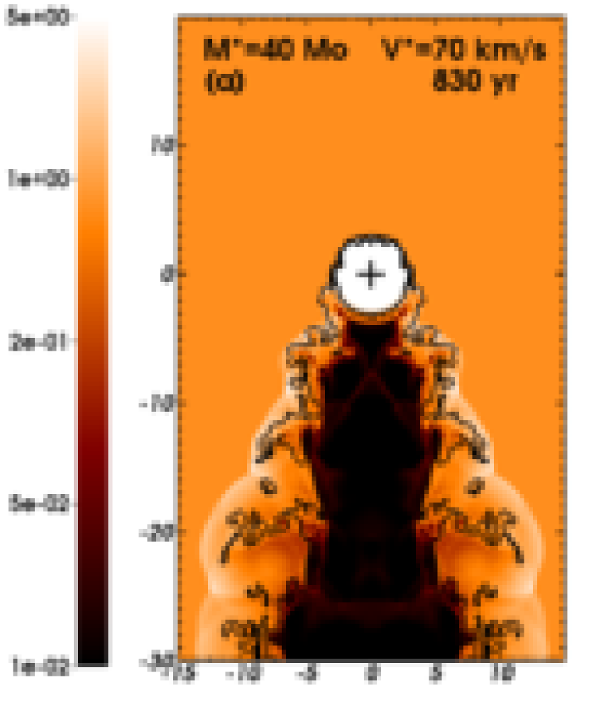
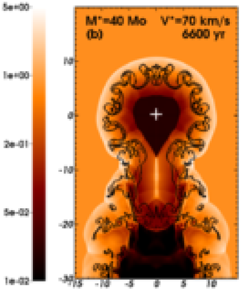
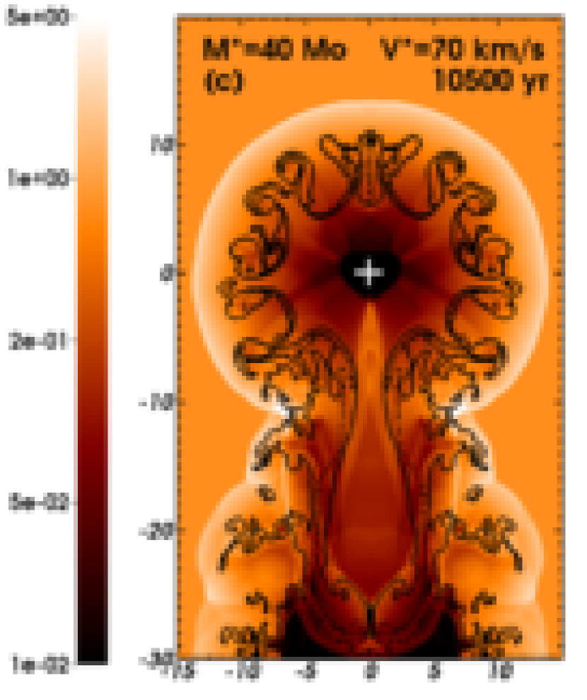
Figure 12: As Fig. 10, with space velocity $v_{\star}=70\,\rm km\,\rm s^{-1}$.

A transmitted wave penetrates the shocked wind material in the bow shock (Brighenti & D’Ercole, 1994) while a second wave is reflected towards the center of the tunnel. After the passage of the shock wave through the interface that separates the tunnel from the bow shock, its cross-sectional area is locally constricted and accelerates the flow. It is about $1500\,\rm km\,\rm s^{-1}$ at a time $4200\,\rm yr$, about $2750\,\rm km\,\rm s^{-1}$ at a time $8000\,\rm yr$ and decelerates down to $1450\,\rm km\,\rm s^{-1}$ when the shock wave expands further in the tunnel at a time $12000\,\rm yr$ in our simulation OSNR2020 (Fig. 13). The same happens when the reflected waves collide at the center of the tunnel (Fig. 13a-b). At a time $t_{\rm ysnr}$ almost the whole interior of the remnant is shocked by the reflected shock wave, and these multiple reflections induce a strong mixing of ejecta, wind and ISM (see the overlapping of the lines where $Q_{1}(\mn@boldsymbol{r})=Q_{2}(\mn@boldsymbol{r})=1/2$). The Rayleigh-Taylor instabilities developing upstream from the center of the explosion (see, e.g. Fig. 12c) have an origin similar to the ones described in Chevalier et al. (1992), but take place at the interface with the shocked ISM gas. Additionally, the interaction with the thin layer of stellar wind material elongates them up to close to the forward shock (Kane et al., 1999).

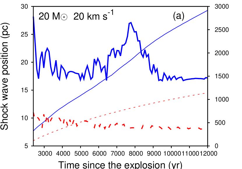
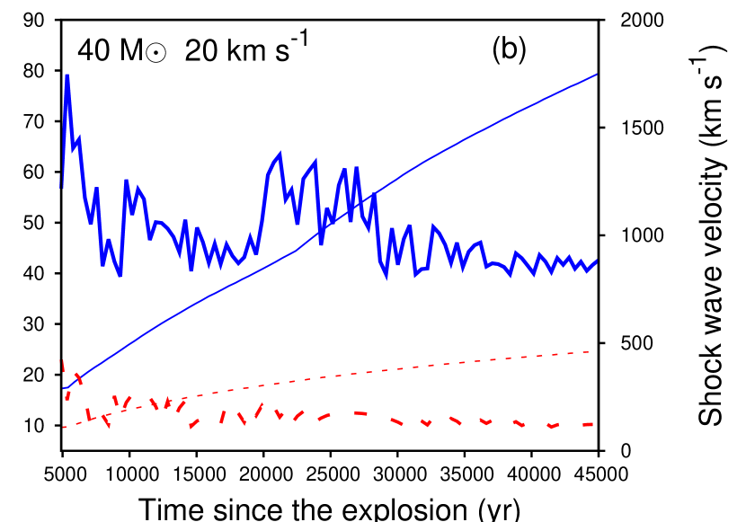
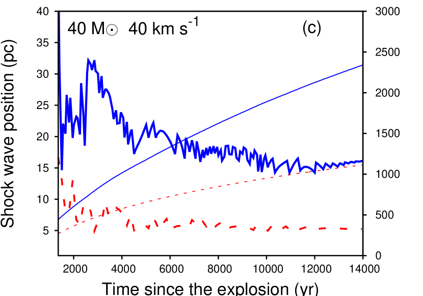
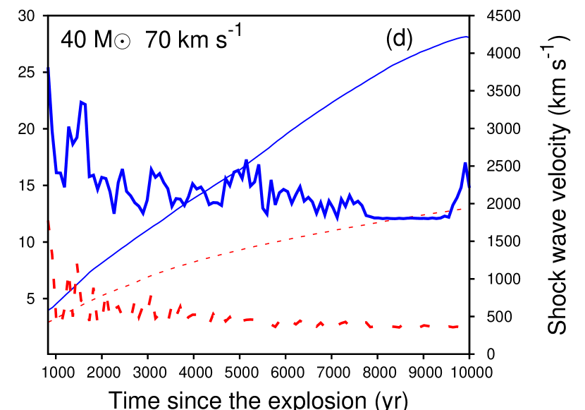
Figure 13: Time evolution of the shock waves of our aspherical supernova remnant models. The figure plots the shock wave position (thin lines, in $\rm pc$) and velocity (thick lines, in $\rm km\,\rm s^{-1}$), measured along the direction of motion of the progenitor, both upstream (dashed red lines, $+\mn@boldsymbol{\hat{z}}$ direction) and downstream (solid blue lines, $-\mn@boldsymbol{\hat{z}}$ direction) from the center of the explosion, respectively. The figure represents the expansion from $t_{\rm ysnr}$ up to the end of the simulation at $t_{\rm osnr}$ (in $\rm yr$) of the remnants generated by our initially $20\,\rm M_{\odot}$ progenitor moving with velocity $20\,\rm km\,\rm s^{-1}$ (a), our initially $40\,\rm M_{\odot}$ progenitor moving with velocity $20$ (b), $40$ (c) and $70\,\rm km\,\rm s^{-1}$ (d), respectively.

The stars end their lives as core-collapse supernovae and the explosion can produce a runaway neutron star (Lyne & Lorimer, 1994). Assuming a typical velocity of the compact object of about $400\,\rm km\,\rm s^{-1}$ (Hobbs et al., 2005), one finds that it could not be further than about $4.84,\,19.8,\,5.6$ and $4.2\,\rm pc$ from the center of the explosion in our simulations at $t_{\rm osnr}$ (Figs. 17c, 10c,  11c and 12c). Consequently, we suggest that our remnants host a neutron star of mass $M_{\rm co}\approx 2\,\rm M_{\odot}$ in the region close to the center of the explosion, i.e. out of the chimney-like extension of channelled ejecta.

5.2 Remnants luminosity

We plot the luminosities (in $\rm erg\,\rm s^{-1}$) of the aspherical supernova remmants as a function of time (in $\rm yr$) in Fig. 14. The bolometric luminosity by optically-thin radiation, $\it L$ (red thin line with triangles), is estimated with the used cooling curve, integrating the energy emitted per unit time and per unit volume over the whole remnant. Similarly, we plot the contribution $L_{\rm ISM}$ from the hot ISM gas ($T>10^{7}\,\rm K$, blue solid line) where radiative losses are mostly due to Bremsstrahlung and from the warm ISM gas ($T\leq 10^{7}\,\rm K$, blue thin dashed lines) where the emission are principally caused by cooling from Helium and metals together with O oxygen forbidden lines emission (see Section 2.4 of Paper I) and the contribution $L_{\rm ej}$ from the ejecta (orange dotted line). We discriminate the various contributions of the luminosity $L$ on the basis of the passive scalars $Q_{1}(\mn@boldsymbol{r})$ and $Q_{2}(\mn@boldsymbol{r})$ advected with the fluid. They allow us to time-dependently trace the proportions of ISM gas, wind and supernova ejecta in the remnants (see section 3.4.1 and Eq. (18) of Paper I). The X-ray luminosity, $L_{\rm X}$, is calculated for gas temperatures $10^{5}\leq T\leq 1.58\times 10^{8}\,\rm K$, with emission coefficients interpolated from tables generated with the xspec software (Arnaud, 1996) with solar metalicity and chemical abundances from Asplund et al. (2009), as in Mackey et al. (2015).

The total luminosity $L$ is first dominated by the hot ($T\geq 10^{7}\,\rm K$) emission from the shocked gas before becoming dominated by emission from the warm ISM gas of temperature $T\leq 10^{7}\,\rm K$ at a time about $8000\,\rm yr$ (see thick solid blue line in Fig. 14a-d) because the post-shock temperature at the shock wave decreases during the adiabatic expansion of the blastwave. The cooling from the metals is stronger at $T\approx 10^{6}\,\rm K$ than at $T\geq 10^{7}\,\rm K$ (Fig.4a of Paper I), so $L$ increases at larger times.

$L$ increases as a function of time from $t_{\rm ysnr}$ up to the end of our simulation. The reflection of the shock wave towards the center of the explosion produces a growing hot, dense region that is upstream from the center of the explosion and augments the luminosity. The emission is influenced by the size of the bow shock at the pre-supernova phase which decreases with $v_{\star}$ (Paper I) and governs the reflection of the shock wave towards the center of the explosion. $L$ monotonically increases by less than one order of magnitude over a timescale of about $10^{4}\,\rm yr$, e.g. in our model OSNR4070 $L\approx 1.2\times 10^{36}\,\rm erg\,\rm s^{-1}$ at $t\approx 10^{3}\,\rm yr$ and $L\approx 9.5\times 10^{36}\,\rm erg\,\rm s^{-1}$ at a time $10^{4}\,\rm yr$ (Fig. 14d).

$L_{\rm ej}$ is smaller than $L_{\rm ISM}$ by a factor of a few at $t_{\rm ysnr}$, e.g. just after the end of the shock wave-bow shock collision, $L\approx 8.0\times 10^{35}$ and $L_{\rm ej}\approx 3.0\times 10^{35}\,\rm erg\,\rm s^{-1}$ in model OSNR4070 (Fig. 14d). It monotonically decreases with time as the shocked ejecta expands and its density decreases such that its emission finally becomes a negligible fraction of $L$ (Fig. 14a-d). The contribution from the wind material is negligible compared to the bolometric luminosity. It is not shown in Fig. 14 since it does not influence $L$ at all.

The total X-ray emission, $L_{\rm X}$, is calculated as the emission from photons at energies $0.1$-$50\,\rm keV$. Not surprisingly, this is slightly smaller than the component of $L_{\rm ISM}$ from the gas with $T\leq 10^{7}\,\rm K$ and follows the same trend as $L$ (Fig. 14a-d). The soft X-ray emission, i.e. from photons in the $0.5$-$1.0\,\rm keV$ energy band, is fainter than $L_{\rm X}$ by less than an order of magnitude and has a similar behaviour as a function of time except for our older and larger supernova remnant OSNR4040 (Fig. 14b). The hard X-ray emission in the $2.0$-$5.0\,\rm keV$ energy band is fainter than $L_{\rm X}$ by about an order of magnitude at $t_{\rm ysnr}$. It decreases as a function of time (Brighenti & D’Ercole, 1994) because the emission of very energetic X-ray photons ceases as the remnant expands and cools. Consequently, our old remnants are more likely to be observed in the soft energy band of X-ray emission.

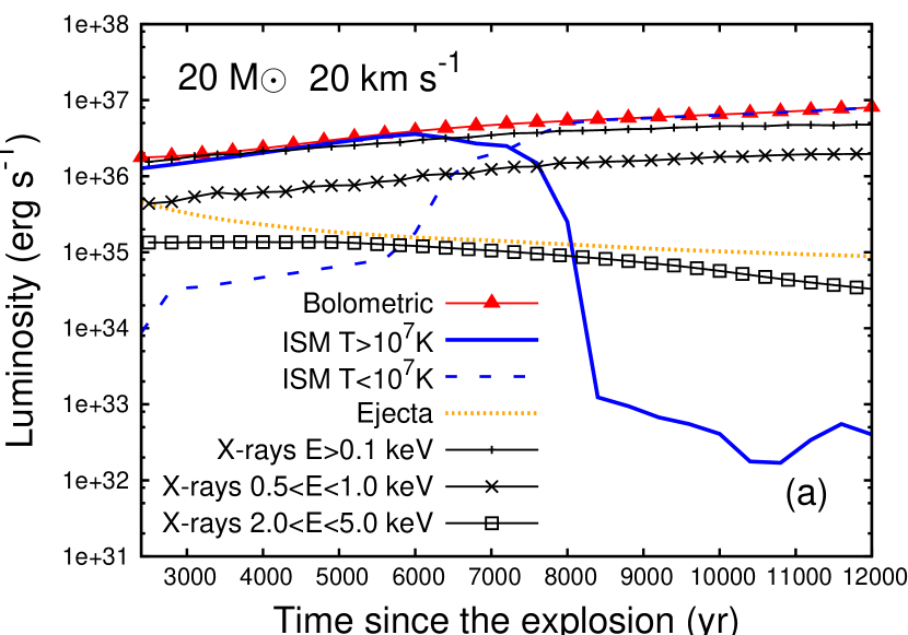
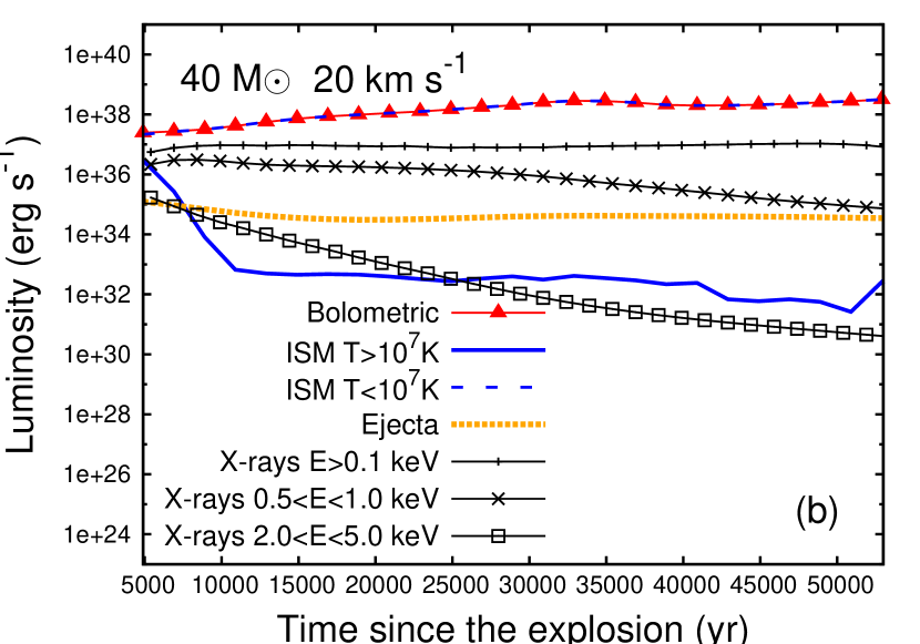
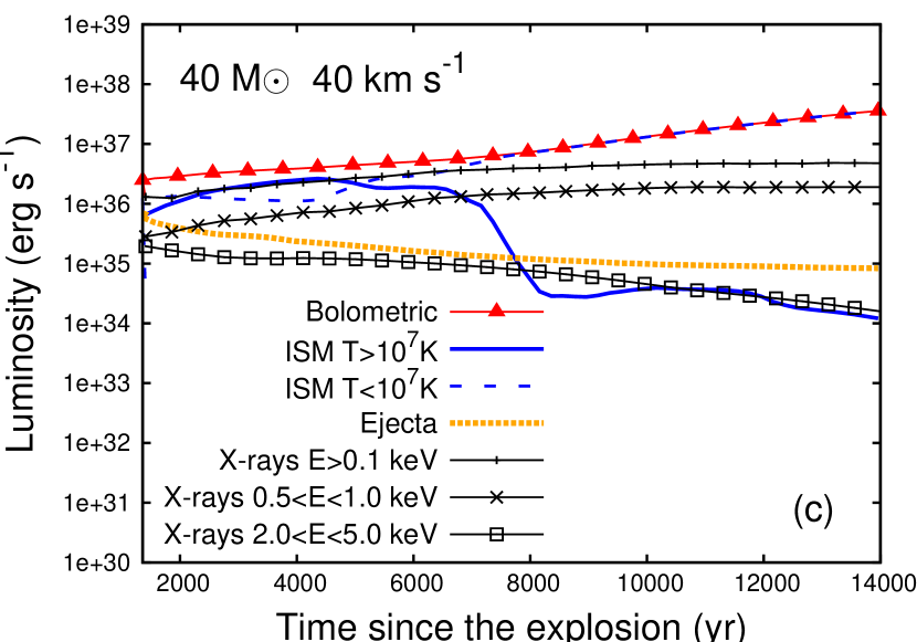
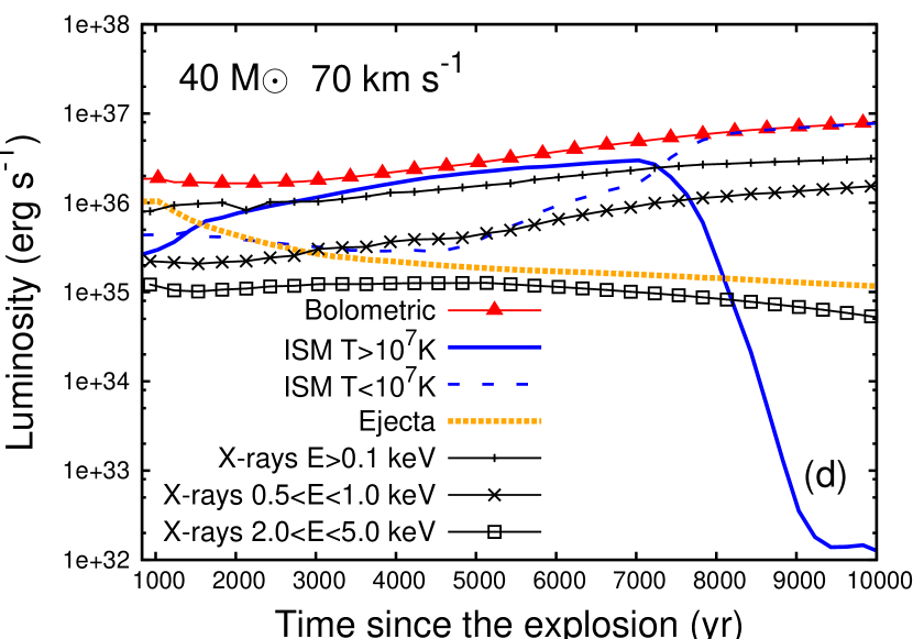
Figure 14: Lightcurves of our old apherical supernova remnants. We show the luminosities (in $\rm erg\,\rm s^{-1}$) during the time interval [$t_{\rm ysnr}$,$t_{\rm osnr}$] (in $\rm yr$) of our aspherical supernova remnants generated by our initially $20\,\rm M_{\odot}$ progenitor moving with velocity $20\,\rm km\,\rm s^{-1}$ (a), our initially $40\,\rm M_{\odot}$ progenitor moving with velocity $20$ (b), $40$ (c) and $70\,\rm km\,\rm s^{-1}$ (d), respectively. The figures distinguish between the bolometric (total) luminosity from the gas (red thin line with triangles), the contribution from the hot ISM gas ($T>10^{7}\,\rm K$, blue solid line), from the warm ISM gas ($T\leq 10^{7}\,\rm K$, blue thin dashed lines) and the contribution from the ejecta (orange dotted line). The black lines are the X-ray luminosity calculated at photons energies $E>0.1\,\rm keV$ ($T>1.2\times 10^{6}\,\rm K$, dashed line), in the soft energy band $0.5$-$1.0\,\rm keV$ ($5.8\times 10^{6}<T<1.2\times 10^{7}\,\rm K$, crossed line) and hard energy band $2.0$-$5.0\,\rm keV$ ($2.3\times 10^{7}<T<5.8\times 10^{7}\,\rm K$, squared line), respectively.

5.3 Emission maps

In Fig. 15 we show synthetic emission maps corresponding to the time $t_{\rm osnr}$ of the supernova remnants generated by our $20\,M_{\odot}$ progenitor moving with $v_{\star}=20\,\rm km\,\rm s^{-1}$ (panels a,d) and by our $40\,\rm M_{\odot}$ progenitor moving with $v_{\star}=20$ (panels b,e) and $40\,\rm km\,\rm s^{-1}$ (panels c,f), respectively. Fig. 16 is similar for our $40\,\rm M_{\odot}$ progenitor moving with $v_{\star}=70\,\rm km\,\rm s^{-1}$. The left-hand side of each panel plots the H$\alpha$ surface brightness (blue) whereas the right-hand side shows the [Oiii] $\lambda\,5007$ surface brightness (green). The left-hand side of each bottom panel plots the hard X-ray surface brightness (red) and the right-hand side shows the soft X-ray surface brightness (grey). The spectral line emission coefficients are taken from the prescriptions by Osterbrock & Bochkarev (1989) and Dopita (1973) for H$\alpha$ and [Oiii] $\lambda\,5007$, respectively, with solar oxygen abundance (Lodders, 2003) and imposing a cut-off temperature at $10^{6}\,\rm K$ (cf. Cox et al., 1991) when oxygen becomes further ionized (Sutherland & Dopita, 1993).

The region of maximum H$\alpha$ surface brightness is located downstream from the center of the explosion. This happens because the H$\alpha$ emissivity, $j_{\rm H\alpha}\propto T^{-0.9}$, is very faint in the region of hot shocked ejecta (Fig. 15a-c). The simulation with the slowly moving $40\,\rm M_{\odot}$ progenitor has an emissivity peak along the walls of the wind cavity (Fig. 15b) because effective cooling of the gas makes the the post-shock region cool ($T\gtrsim\,10^{4}\,\rm K$) and dense (up to $n\approx 50\,\rm cm^{-3}$). In the other simulations, the emission originates from the outer layers of the bow shocks because the walls of their less massive bow shocks allow a faster and deeper penetration of the shock wave into the shocked wind material (Fig. 16). Our predicted maximum H$\alpha$ emission is above the diffuse emission sensitivity limit of the SuperCOSMOS H-alpha Survey (SHS Parker et al., 2005) of $1.1$$-$$2.8\times 10^{-17}\,\mathrm{erg}\,\mathrm{s}^{-1}\,\mathrm{cm}^{-2}\,\mathrm{arcsec}^{-2}$, e.g. our model OSNR4040 has a maximum emission larger than $9\times 10^{-16}\,\mathrm{erg}\,\mathrm{s}^{-1}\,\mathrm{cm}^{-2}\,\mathrm{arcsec}^{-2}$ (Fig. 15b), and could be compared with data from these surveys.

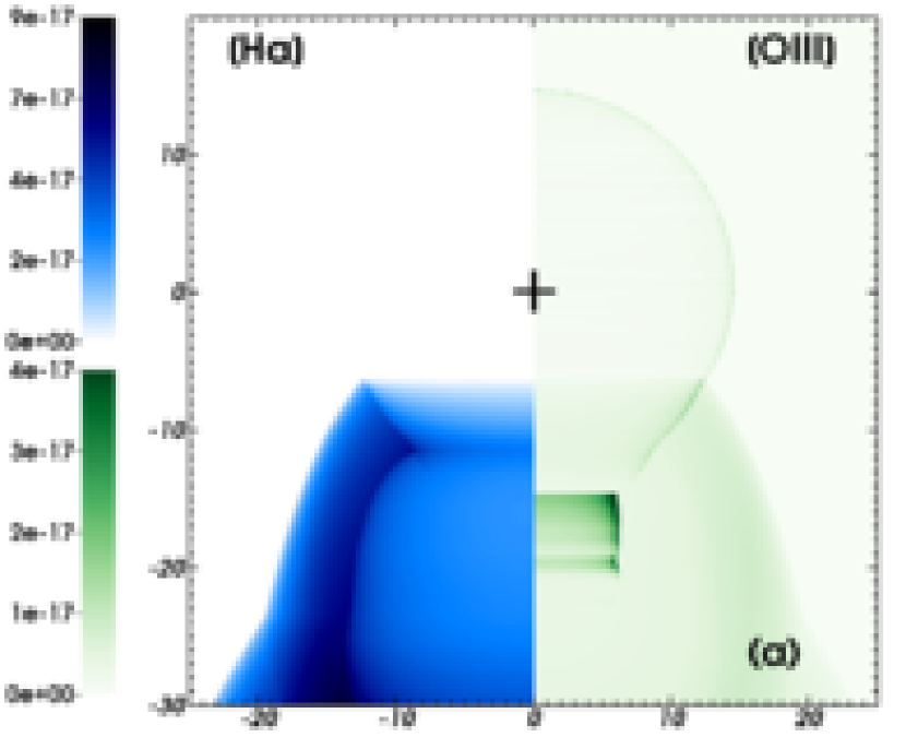
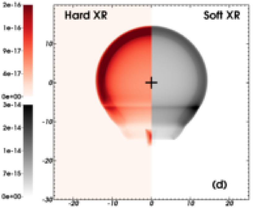
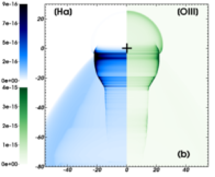
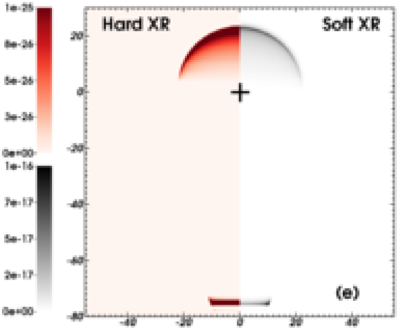
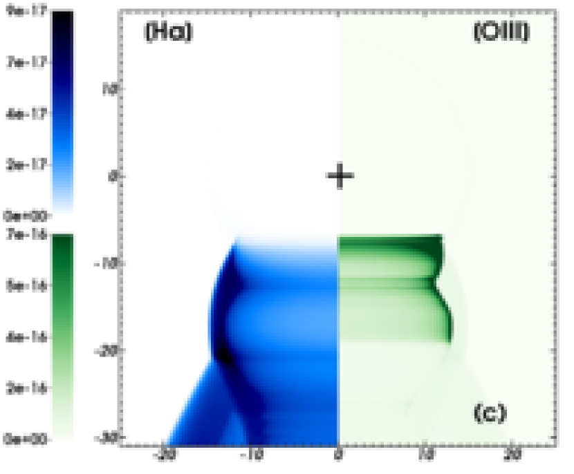
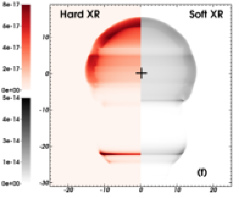
Figure 15: Synthetic emission maps of our models OSNR2020 at a time $12100\,\rm yr$ (a,d), OSNR4020 at time $49500\,\rm yr$ (b,e) and OSNR4040 at a time $14000\,\rm yr$ (c,f), plotted on the linear scale in units of $\rm erg\,\rm s^{-1}\,\rm cm^{-2}\,\rm arcsec^{-2}$. The left-hand part of the figures show the H$\alpha$ surface brightness (blue) and the right-hand part the [Oiii] surface brightness (green), respectively. The black crosses mark the center of the explosion. The panels d-f show the projected X-ray emission maps in the hard ($2.0$-$5.0\,\rm keV$  corresponding to $2.3\times 10^{7}<T<5.8\times 10^{7}\,\rm K$, left-hand part) and soft ($0.5$-$1.0\,\rm keV$ corresponding to $5.8\times 10^{6}<T<1.2\times 10^{7}\,\rm K$, right-hand part) X-ray bands for the same models. The $x$-axis represents the radial direction and the $y$-axis the direction of stellar motion (in $\mathrm{pc}$). Only part of the computational domain is shown in the figures.

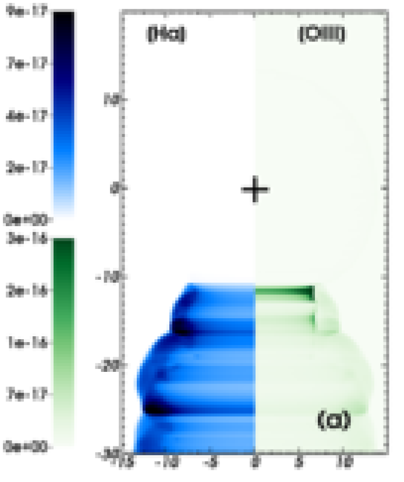
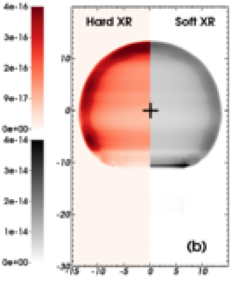
Figure 16: As Fig. 15, with an initially $40\,\rm M_{\odot}$ progenitor moving with space velocity $v_{\star}=70\,\rm km\,\rm s^{-1}$. The H$\alpha$ and [Oiii] $\lambda\,5007$ surface brightnesses are plotted in the left-hand panel, the projected hard and soft X-ray emissivity in the right-hand panel.

The [Oiii] maximum surface brightness of our models originates from the dense ($n\approx 2$$-$$10\,\rm cm^{-3}$) and warm ($T\leq 10^{6}\,\rm K$) post-shock region behind the shock wave. It is located at the walls of the cavity and produces a ringed/tubular structure (Fig. 15a-c and 16a). It is generally not coincident with the projected H$\alpha$ emission because the [Oiii] emissivity has a different dependence on the temperature, i.e. $j_{\rm{[O{{\sc III}}]}}\,\propto\,e^{-1/T}/T^{1/2}$. However, the simulation OSNR4020 with a heavy bow shock have its [Oiii] maximum surface brightness all along the walls of the wind tunnel and it is coincident with the region of maximum H$\alpha$ emission, i.e. the behaviour of the emissivities with respect to the large compression of the gas in the walls ($\propto n^{2}$) overwhelms that of the gas temperature (Fig. 15b).

The X-ray emission originates from the hot gas with $10^{5}\leq T\leq\,10^{8}\rm K$, i.e. from near the shock wave expanding into the unperturbed ISM. The maximum surface brightness comes from the hot region of doubly shocked gas upstream from the center of the explosion, and from the post-shock region at the channelled shock wave (Figs. 15d-f, 16b). The hard X-ray surface brightness is several orders of magnitude fainter than the projected soft X-ray emission, because the gas is not hot enough at $t_{\rm osnr}$ (Fig. 14). The emitting region in soft X-rays is peaked in the post-shock region at the shock wave whereas the hard X-ray come from a broader region of shocked gas which outer border is the shock wave (Fig. 15f). Note also the anti-correlation between the surface brightness in X-ray (hot region from near the forward shock) and in [Oiii] (colder and denser walls) in our remnants generated by a fast-moving ($v_{\star}\geq 40\,\rm km\,\rm s^{-1}$) progenitor (Fig. 15b,e;c,f).

6 Discussion

We here discuss our results in the light of precedent studies and pronounce on the best manner to observe aspherical supernova remnants generated by massive Galactic runaway stars. Finally, we examine our models in the context of recent observations.

6.1 Comparison with previous works

We tested that the code pluto (Mignone et al., 2007, 2012) reproduced the one-dimensional models of core-collapse supernovae interacting with their surroundings in Whalen et al. (2008) and van Veelen et al. (2009) using a uniform, spherically symmetric grid. Our numerical method (Paper I) is different from that in Whalen et al. (2008) because (i) they utilise a finite-difference scheme coupled to a network of chemical reactions following the non-equilibrium rates of the species composing the gas and (ii) their algorithm includes artificial viscosity (zeus code, see Stone & Norman, 1992).

We ran tests with their cooling curve (MacDonald & Bailey, 1981) and with a cooling curve for collisional ionization equilibrium medium (see details in section 2.4 of Paper I). We find no notable differences, mostly because they are similar in the high temperature regime ($T\geq 10^{5}\,\rm K$) that is relevant for the supernova-wind interaction (Fig. 5). We extend this method to two-dimensional, cylindrically symmetric tests of a supernova shock wave expanding into a homogeneous ISM to ensure that the sphericity of the shock wave is conserved throughout its expansion. We notice that the solution behaves well with respect to the symmetry axis $Oz$.

Models of an off-centered explosion in a wind-driven cavity are available in Rozyczka et al. (1993). Their model produces a parsec-scale jet-like feature as do our aspherical models (Figs. 17c to 12c) but they neglect the progenitor’s stellar evolution, assume a different microphysics, and correspond to a totally different point of the parameter space ($n=10^{6}\,\rm cm^{-3}$). Our description of the supernova shock wave interacting with its pre-shaped bow shock is consistent with the works tailored to the Kepler’s supernova remnant; see section 5.2 of Borkowski et al. (1992) but also Velázquez et al. (2006); Toledo-Roy et al. (2014).

The tunnel of unshocked wind that channels the shock wave, e.g. in our model OSNR4020 (Fig. 17a), is morphologically and structurally consistent with the model of the red supergiant progenitor of the Crab nebula in Cox et al. (1991), assuming a diluted ambient medium and a larger space velocity ($n=0.25\,\rm cm^{-3}$, $v_{\star}=69.5\,\rm km\,\rm s^{-1}$). Notice that the simulations with fast-moving stars or post-main-sequence high-mass-loss events have a tunnel with clumpy walls (Fig. 17a and 12a) which do not prevent the tunneling of the shock, in contrast to the suggestion by Cox et al. (1991).

The growth and overall shape of our aspherical remnants are in accordance with Brighenti & D’Ercole (1994). Our model OSNR2020 is morphologically consistent with their model 1 ($v_{\star}=17\,\rm km\,\rm s^{-1}$, $n=1\,\rm cm^{-3}$). They assumed a comparable mass loss ($\dot{M}=10^{-5}\,\rm M_{\odot}\,\rm yr^{-1}$) but a twice larger wind velocity ($v_{\rm w}=20\,\rm km\,\rm s^{-1}$) during the red supergiant phase which lastes about $7\times 10^{5}\,\rm yr$. Identical remarks arise comparing their model 3 and our simulation OSNR4070 (Fig. 12a-c). Because our models include thermal conduction, the region of shocked wind in the bow shock from the main-sequence phase is larger and the tunnel in our simulation OSNR4020 narrower than in their model 4 and allows a more efficient channeling of the shock wave (Fig. 10a-c). More details about the effects of heat conduction in our remnants is given in Appendix A.

As a conclusion, for overlapping parameters our results agree well with previous models of supernova remnants produced by runaway progenitors. We extend the parameter space with a representative sample of models tailored to the Galactic plane, whose progenitor’s wind properties are taken from self-consistently pre-calculated stellar evolution models (Brott et al., 2011).

6.2 Comparison with observations

6.2.1 General remarks and comparison approach

Comparing our simulations with observations is not a straightforward task. Even though this paper explores a representative sample of Galactic, massive, runaway stars, our remnants can only develop asymmetries when the isotropic shock wave interacts in reality with a dense bow shock, whereas other mechanisms can also induce asymmetries. They can originate from an intrinsically anisotropic explosion (Blondin et al., 1996), the rotation of the progenitor (Langer et al., 1999), the magnetization of the ISM (Rozyczka & Tenorio-Tagle, 1995) or the presence of a neighbouring circumstellar structure (Ferreira & de Jager, 2008). Consequently, we hereby simply attempt to establish a qualitative discussion between the density fields in our models and observations available in the literature.

Supernova remnants are often observed in radio wavelengths (Green, 2009), e.g. at about $325$, $843$ or $1400\,\rm Mhz$. This emission arises from bremsstrahlung (proportional to $n_{e}^{2}$, where $n_{e}$ is electron number density ), synchrotron radiation (proportional to $n_{e}B$, where $B$ is the field strength), and maser emission (tracing very dense ISM regions). Our discussion is limited to a simple comparison between such published measures and the density fields in our hydrodynamical simulations. Additionally, because Galactic SNRs usually have poorly constrained distances (and hence sizes and masses), we discuss morphological similarities even though it may not be clear whether or not our model parameters are appropriate to a given observed remnant.

6.2.2 Observations from maser emission such as in 3C391: explosions in a dense medium, runaway progenitors or both ?

Brighenti & D’Ercole (1994) and Eldridge et al. (2011) already justified the relevance of studying runaway O stars in the understanding of supernova remnants and gamma-rays bursts. Particularly, they underline the difficulty of interpreting the shape of incomplete and/or inhomogeneous arc-like supernova remnants because the overdensities upstream from the center of the explosion can also arise from pre-existing dense regions (see, e.g. Orlando et al., 2008). The presence of OH maser emission originating from the shock front can discriminate between these scenarios (Frail et al., 1996; Yusef-Zadeh et al., 2003), and led to the classification of about $20$ Galactic arced remnants such as G31.9+0.0 or G189.1+3.0 as running into a dense cloud.

Examining the necessary conditions to produce OH $1720\,\rm{\color[rgb]{0,0,0}Mhz}$ ($T\approx 50$-$125\,\rm K$, $n_{\rm medium}\approx 10^{5}\,\rm cm^{-3}$, OH column density $N_{\rm OH}\approx 10^{16}\,\rm cm^{-2}$, see Lockett et al. 1999) one finds that such high densities are not reached in our models. However, according to the Rankine-Hugoniot jump relations it may be the case in the post-shock region if the shock propagates in a medium of pre-shock density $n_{\rm medium}/4\approx 2.5\times 10^{4}\,\rm cm^{-3}$ such as a starless dense core, a molecular cloud or a contracting ISM filament (Kaufman & Kaufman, 2009). Assuming a temperature of $T\approx 50\,\rm K$, the medium sound speed is $c_{\rm s}\approx 0.65\,\rm km\,\rm s^{-1}$ so any star moving with velocity $v_{\star}\approx 5c_{\rm s}\approx 3.25\,\rm km\,\rm s^{-1}$ would have an hypersonic motion and produce a bow shock. Consequently, if OH maser emission is not likely to be detected from bow shocks in the field, it naturally arises from the surroundings of runaway stars in a dense medium. Moreover, if the star explodes in such an environment, additional constraints may be necessary in order to distinguish between maser emission produced because of the runaway nature of the progenitor, emission originating from an expanding shock wave, or both.

Particularly, 3C391 was originally believed to be the archetypal remnant from a moving progenitor (Brighenti & D’Ercole, 1994) but is now known to be associated with OH maser emission (Frail et al., 1996) together with molecular line emission. The Infrared Spatial Observatory (ISO) revealed, among other, CO, HC$\rm O^{+}$ line emission (see Reach & Rho, 1999, and references therein) whereas Neufeld et al. (2014) reported recent infrared analysis of the $\rm H_{2}$ and $\rm H_{2}$O line emission. However, as mentioned above, nothing indicates whether this emission originates from the shock wave colliding with a wind bubble produced by the progenitor or from the shock wave running into its dense surrounding medium. Modelling the explosion of a supernova from a runaway progenitor with $n_{\rm medium}\gg 1\,\rm cm^{-3}$ is conceivable but beyond the scope of the present investigation and left for a follow-up study. Considering the past evolution of supernova progenitors in the modelling of their remnants will help to discriminate between these two situations. Further investigations, e.g. tailored to 3C391, may provide more severe constraints on its circumstellar medium at the pre-supernova phase and help to understand its formation scenario.

6.2.3 Bilateral supernova remnants

Our simulations PSN4020 and PSN4040 produce approximately cylindrical wind-blown cavities with dense walls. The interaction of the supernova with this circumstellar medium, in our models OSNR4020 and OSNR4040 (Figs. 10 and 11) produces the conditions required for a bilateral supernova remnant, i.e. a cylindrical cavity with dense, shocked gas on the boundaries. A previous study identified the material composing the bilateral structures of the remnant G296.5+10.0 as shocked pre-supernova wind (Manchester, 1987) and the presence of a neutron star in between the opposed arcs is reported in Zavlin et al. (1998). It constrains the stellar remnant to be a $1.4\,\rm M_{\odot}$ neutron star, so its progenitor had initial mass below about $25\,\rm M_{\odot}$ (Woosley et al., 2002). It is similar to our slowly moving model of an initially $40\,\rm M_{\odot}$ at time $11400\,\rm yr$ after the explosion, when the shock wave hits the very dense walls of the wind tunnel (Fig. 10b). Our understanding of the bilateral character of this remnant as a result of its progenitor’s supersonic motion only is valid if one considers a lower initial mass progenitor moving in a medium dense enough to form heavy cavity walls resistant to the shock wave. Note that this result is consistent with fig. 6D of Orlando et al. (2007).

However, alternative explanations have been proposed for the fomation of bilateral remnants like G327.6+14.6 or G3.8-0.3. A strong axisymmetric background ISM magnetic field (not included in our simulations) has also been suggested to be responsible for the bilateral character of some Galactic supernova remnants (Gaensler, 1998). It would indeed make their shape more elongated as long as the field is strong enough (Rozyczka & Tenorio-Tagle, 1995) and produce X-ray and/or radio synchrotron emission from the opposed arcs (Velázquez et al., 2004; Petruk et al., 2009; Schneiter et al., 2010).

6.2.4 The jet/tubular-like extension shaped by the motion of the progenitor

Our Galactic, slowly moving, initially $20\,\rm M_{\odot}$ progenitor produces a supernova remnant whose outer region strongly emits in [O iii]. The remnant generated by our slowly moving, initially $40\,\rm M_{\odot}$ progenitor has an [O iii] jet-like feature that has a H$\alpha$ counterpart (Fig. 15) generated by ejecta channelled with velocity about $1000\,\rm km\,\rm s^{-1}$ into the wind tunnel of the bow shock (Fig. 13b). Those tubular/jet-like features (Figs. 15-16) are reminiscent of the chimney discovered in [Oiii] in the Crab nebula (Blandford et al., 1983) modeled in Cox et al. (1991). This morphological resemblance mostly arises because of the similar stellar evolution history and space velocity $v_{\star}\approx 30\,\rm km\,\rm s^{-1}$ in both simulations.

Nevertheless, further investigations and detailed comparison would have to take into account the youth of the Crab nebula ($\approx 1000\,\rm yr$) and its location in the high latitude, low-density ISM of the Galaxy. In our simulations with larger $v_{\star}$, those jet-like extensions become an [O iii] tubular structure that is thinner and closer to the throttling separating the surroundings of the center of the explosion from the trail of the bow shock. Supernovae exploding in a wind cavity could hence form tunnels or barrel-like shapes, however, alternative quite convincing demonstration, e.g. based on asymmetric explosions have already been proposed (WB49, González-Casanova et al., 2014).

6.2.5 An alternative explanation for the Cygnus loop nebula ?

G074.0-8.5, also called the Cygnus loop, is a supernova remnant for which X-ray observations, e.g. with ROSAT (Aschenbach & Leahy, 1999) reveal a characteristic overall drop-like morphology. An early interpretation of this shape is a champagne blowout from the edge of a molecular cloud (Tenorio-Tagle et al., 1985). Recent X-ray data favours a model with an explosion into a pre-shaped cavity and whose ejecta have recently impacted the imperfect walls.  Uchida et al. (2009) supports this model and derives the remnant’s age to be about $10000\,\rm yr$, its radius to be $12$-$17\,\rm pc$ and its initial progenitor’s mass to be $12$-$15\,\rm M_{\odot}$, which is consistent with our model OSNR2020 (Fig. 15d).

Moreover, some southern optical filaments have a measured expansion velocity of a few hundred $\rm km\,\rm s^{-1}$ (Medina et al., 2014) as in our simulation OSNR2020 (Fig. 13a). In our picture, the south blowout region of the remnant is the low-density wake behind the progenitor in which the gas is the hottest ($>10^{6}\,\rm K$), as noted in Aschenbach & Leahy (1999). Nevertheless, our models predict that the soft and hard X-rays emission should be limb-brightened, whereas the observations have a filled morphology. This may be explained by the presence of a neutron star (Katsuda et al., 2012) that is not taken into account in our models. Future simulations, investigating the plerionic nature of the Cygnus loop nebula will allow us to assess this interpretation.

6.2.6 Distinguishing remnants from moving progenitors and remnants with ISM-induced anisotropy.

Distinguishing whether a one-sided supernova remnant is produced thanks to the motion of its progenitor or because of its surroundings’ inhomogeneity is difficult since both situations can happen together. As discussed above, the OH emission can trace the presence of a molecular cloud, but is not sufficient to exclude the presence of an hypothetical bow shock. A couple of additional comments can be given.

1. In the situation of a runaway supernova progenitor, the cavity that channels the subsequent shock wave left behind its bow shock may produce a more collimated remnant than in the case of an interaction with a dense cloud. This phenomenon could be enhanced by the presence of a background ISM magnetic field which elongates the pre-shaped tunnel, reducing the instabilities affecting its walls and consequently favoring the channeling.

2. If a runaway massive star sheds (an) heavy envelope(s) throughout its evolution, e.g. via a luminous blue variable event or a Wolf-Rayet phase, the passage of the shock wave through these expelled shell(s) will fragment them. Their temperature will increase by shock heating before cooling down, inducing an X-ray rebrightning of the formed foculli. Such a mixed-morphology supernova remnant generated by a blown bow shock would have an incomplete arc-like radio envelope around a central region containing X-ray-emitting clumps.

3. The situation becomes more complicated when the explosion happens at the interface between two different phases of the ISM. If a runaway progenitor leaves a molecular cloud, the tubular extension produced by the channeled shock wave will be directed towards the center of the cloud. If the progenitor enters the cloud, the imprint of the last mass-loss events of the moving star onto the border of the cloud will produce a characteristic hole. A famous (nonetheless extragalactic) example of such a phenomenon is the structure that overhangs the remnant of SN1987a in the Large Magellanic Cloud (Wang et al., 1993).

7 Conclusion

In this paper, we present a grid of hydrodynamical models of asymmetric supernova remnants generated by a representative sample of Galactic runaway massive stars whose circumstellar medium during the main-sequence and red supergiant phases is studied in Meyer et al. (2014). We compute the bow shocks generated by our progenitors from near the pre-supernova phase and model the collision between the supernova shock waves and the circumstellar medium which result in the generation of supernova remnants. The progenitors’ initial masses range from $10$ to $40\,\rm M_{\odot}$ and they move with space velocities ranging from $20$ to $70\,\rm km\,\rm s^{-1}$. Our models include both optically-thin cooling and photoheating of the gas. Electronic thermal conduction is included in the calculations of the circumstellar medium and in the simulations of the supernova remnants.

We stress that the stellar motion of a core-collapse supernova progenitor can be responsible for the deviations from sphericity of its subsequent remnant. We show that the bow shocks trapping at least $1.5\,\rm M_{\odot}$ of ISM gas are likely to generate aspherical supernova remnants. They correspond to high mass and/or slowly moving stars (Brighenti & D’Ercole, 1994; Meyer et al., 2014). At the ISM number density that we consider, they are produced either by our initially $20\,M_{\odot}$ star moving with space velocity of about $20\,\rm km\,\rm s^{-1}$ or by our initially $40\,\rm M_{\odot}$ runaway star. These mass-accumulating bow shocks generate a dense bulge of shocked ISM gas upstream from the direction of motion of the star whereas a cavity of low-density wind material forms in the opposite direction and extends as a tunnel of unshocked wind material into the trail of the bow shock.

After the supernova explosion, the shock wave expansion is strongly influenced by the anisotropy of its circumstellar medium. It collides with the overdense part of the bow shock whereas it expands freely at velocities of the order of $1000\,\rm km\,\rm s^{-1}$ in the opposite direction, channelled by the pre-shaped tunnel of unshocked wind material (cf. observations of RCW86 in Vink et al., 1997). The mass of shocked ISM trapped in the bow shock decelerates the shock wave, which continues to penetrate the unperturbed ISM after the collision with velocity of the order of $100\,\rm km\,\rm s^{-1}$.

As the shock wave evolves in a non-uniform medium, it is partly reflected towards the center of the explosion (Ferreira & de Jager, 2008) after the collision with a dense bow shock. It induces mixing of supernova ejecta, stellar wind and ISM gas that is particularly important for fast-moving progenitors. This reflected wave shocks the zone around the center of the explosion, reheating the gas, which subsequently cools below $10^{7}\,\rm K$ because of the adiabatic expansion of the blastwave. Its luminosity increases, dominated by thermal Bremsstrahlung and soft X-ray emission originating from the shocked ISM that is upstream from the center of the explosion. The emission from the ejecta or from the progenitor’s wind material does not contribute significantly to the remnants’ total luminosity once the bow shock is overtaken by the supernova shock wave.

Our Galactic aspherical supernova remnants have an [Oiii] $\lambda\,5007$ surface brightness larger than their projected H$\alpha$ emission, i.e. the [Oiii] is more appropriate line to search for Galactic supernova remnants. Their [Oiii] surface brightness is maximum in the post-shock region of the shock wave. It is concentrated along the walls of the tunnel of wind material. The region of maximum H$\alpha$ emission is downstream from the direction of motion of the progenitor. It originates from the outer part of shocked ISM material in the trail of the progenitor’s bow shock. In the case of our slowly moving initially $40\,\rm M_{\odot}$ progenitor, it mainly comes from the region where the shock wave interacts with the walls of the tunnel, i.e. the ejecta forms an [O iii] tubular-like feature that has an H$\alpha$ counterpart. Moreover, we find that our remnants are brighter in soft X-ray emission originating from near the shock wave than in hard X-ray emission coming from the post-shock region at the shock wave.

Supernova remnants generated by runaway progenitors naturally show structures highly deviating from sphericity. Particularly, our models of remnants generated by high-mass, slowly moving progenitors have morphologies consistent, e.g. with the bilateral character of observed barrel-like Galactic supernova remnants such as G296.5+10.0 or with the morphology of the Cygnus loop nebula. However, other mechanisms are at work in the shaping of supernova remnants. Forthcoming work will investigate the effects of an ISM magnetic field on the evolution of our remnants, in order to quantitatively appreciate its consequences on the remnants’ dynamics and emission signatures.

Appendix A The effects of thermal conduction

In this Appendix we discuss the effects of thermal conduction on the shape and internal structures of our circumstellar nebulae, before and after the supernova explosion.

A.1 The effects of thermal conduction on the pre-shaped cirumstellar medium

In the situation of our slowly-moving stars ($v_{\star}=20\,\rm km\,\rm s^{-1}$), we have an off-centered explosion inside the wind-bubble generated during the main-sequence phase of the moving star (Brighenti & D’Ercole, 1994). The effects of thermal conduction mainly arise from the structural differences it induces in the bow shock, which consist in the circumstellar medium of the star at the pre-supernova phase (see our model PSN4020 in Fig. 17a). The high effective temperatures of our main-sequence, massive stars produce a heat flux which timescale $\propto T^{-7/2}$ (Orlando et al., 2005, Paper I) is much faster than both the dynamical advection timescale of the stellar wind and ISM gas in the bow shock and cooling by optically-thin radiative processes timescale. It transports large amount of the gas internal energy from the reverse shock of the bow shock towards the contact discontinuity that slightly enlarges the bow shock in the direction of motion of the star. Moreover, it damps the instabilities developing at the reverse shock, i.e. the walls of the tunnel, and reorganises its internal structure (see discussion in section 3.3 of Paper I).

In the case of our fast-moving stars ($v_{\star}\geq 40\,\rm km\,\rm s^{-1}$), we have an off-centered explosion outside the wind-bubble generated during the main-sequence phase of the moving star and the supernova explosion consequently takes place in a pre-shaped circumstellar medium where any information relative to the main-sequence wind bubble is located behind the star (Brighenti & D’Ercole, 1994). The effects of thermal conduction mainly arise from the instabilities that develop in the bow shock produced during the post-main sequence phase of the stellar evolution. Since the seeds and the growth of the Kelvin-Helmholtz and Rayleigh-Taylor instabilities partly depend on density distribution at the end of the main-sequence phase, the effects of thermal conduction consist in changing the shape of the instabilities at the apex of these bow shocks (see our model PSN4070 in Fig. 17b). Note that only the morphology of the eddies at a given time differ, the developing instability remains of the same kind, i.e. a thin-shell-related instability (Vishniac, 1994; Blondin & Koerwer, 1998).

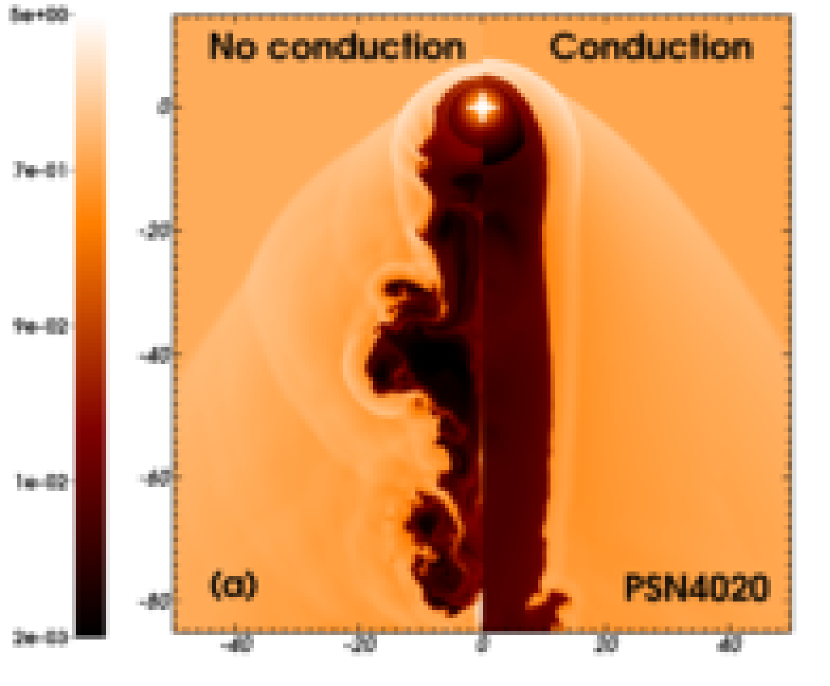
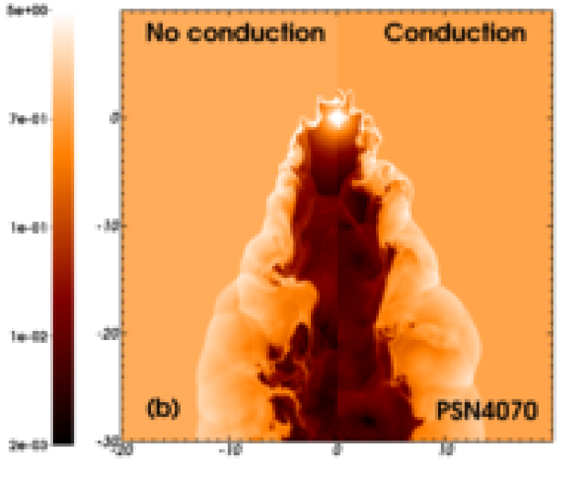
Figure 17: Effects of heat conduction on the pre-supernova circumstellar medium of our initially $40\,\rm M_{\odot}$ progenitor moving with velocity $20\,\rm km\,\rm s^{-1}$ (a) and $70\,\rm km\,\rm s^{-1}$ (b). The figure shows the gas number density field of simulations carried out without (left-hand part of the panels) and with heat conduction (right-hand part of the panels) with a density range from about $10^{-3}$ to $5.0\,\mathrm{cm}^{-3}$ on the logarithmic scale, at a time $t_{\rm osnr}$. The white cross marks the position of the runaway star.

A.2 The effects of thermal conduction on the old supernova remnants

In the situation of our slowly-moving supernova progenitors, the remnant is affected by thermal conduction in the sense that the channeled supernova shock wave interacting with the walls of the cavity encounters a more irregular and clumpy medium (Fig. 18a). It changes neither the shape of the outflow along the direction of the progenitor nor the global remnant’ morphology, however, it may generate ring-like emission artefacts, e.g. by projection effect. Note that heat conduction is in its turn sensitive to the ISM magnetisation which makes it anisotropic (Balsara et al., 2008) as it has been shown in several studies devoted to old supernova remnants (Velázquez et al., 2004; Balsara et al., 2008).

In the case of our fast-moving supernova progenitors, the absence of thermal transfers (i) slightly modify, as discussed above, the shape of the eddies constituting the pre-supernova circumstellar medium distribution and (ii) allows the ejecta interacting with the bow shock to cool independently of the rest of the gas during the radiative phase of the remnant. Consequently, the fingers of the developing Rayleigh-Taylor instabilities become denser (Fig. 18b).

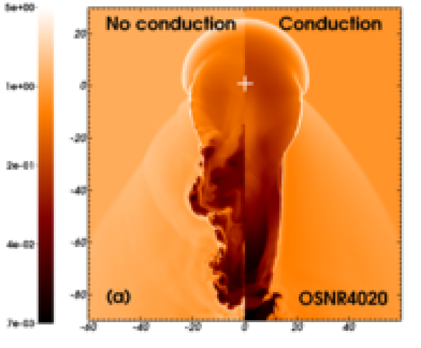
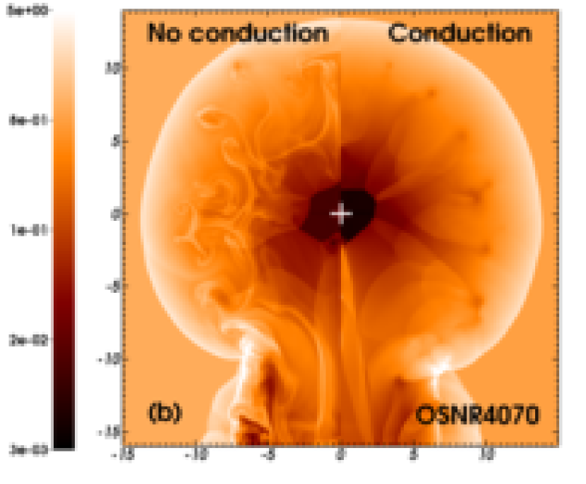
Figure 18: Effects of heat conduction on the old supernova remnant generated by our initially $40\,\rm M_{\odot}$ progenitor moving with velocity $20\,\rm km\,\rm s^{-1}$ (a) and $70\,\rm km\,\rm s^{-1}$ (b). The figure shows the gas number density field of simulations carried out without (left-hand part of the panels) and with heat conduction (right-hand part of the panels) with a density range from about $10^{-3}$ to $5.0\,\mathrm{cm}^{-3}$ on the logarithmic scale, at a time $t_{\rm osnr}$. The white cross marks the center of the explosion.

References

- Abdo et al. (2010) Abdo A. A., Ackermann M., Ajello M., 2010, ApJ, 722, 1303
- Arnaud (1996) Arnaud K. A., 1996, in Jacoby G. H., Barnes J., eds, Astronomical Data Analysis Software and Systems V Vol. 101 of Astronomical Society of the Pacific Conference Series, XSPEC: The First Ten Years. p. 17
- Aschenbach & Leahy (1999) Aschenbach B., Leahy D. A., 1999, A&A, 341, 602
- Asplund et al. (2009) Asplund M., Grevesse N., Sauval A. J., Scott P., 2009, ARA&A, 47, 481
- Baade (1938) Baade W., 1938, ApJ, 88, 285
- Badenes et al. (2010) Badenes C., Maoz D., Draine B. T., 2010, MNRAS, 407, 1301
- Balsara et al. (2008) Balsara D. S., Bendinelli A. J., Tilley D. A., Massari A. R., Howk J. C., 2008, MNRAS, 386, 642
- Balsara et al. (2008) Balsara D. S., Tilley D. A., Howk J. C., 2008, MNRAS, 386, 627
- Baranov et al. (1971) Baranov V. B., Krasnobaev K. V., Kulikovskii A. G., 1971, Soviet Physics Doklady, 15, 791
- Bedogni & D’Ercole (1988) Bedogni R., D’Ercole A., 1988, A&A, 190, 320
- Blaauw (1993) Blaauw A., 1993, in Cassinelli J. P., Churchwell E. B., eds, Massive Stars: Their Lives in the Interstellar Medium Vol. 35 of Astronomical Society of the Pacific Conference Series, Massive Runaway Stars. p. 207
- Blandford et al. (1983) Blandford R. D., Kennel C. F., McKee C. F., Ostriker J. P., 1983, Nature, 301, 586
- Blondin & Koerwer (1998) Blondin J. M., Koerwer J. F., 1998, New Ast., 3, 571
- Blondin et al. (1996) Blondin J. M., Lundqvist P., Chevalier R. A., 1996, ApJ, 472, 257
- Borkowski et al. (1992) Borkowski K. J., Blondin J. M., Sarazin C. L., 1992, ApJ, 400, 222