Modeling sympathetic cooling of molecules by ultracold atoms

Abstract

We model sympathetic cooling of ground-state CaF molecules by ultracold Li and Rb atoms. The molecules are moving in a microwave trap, while the atoms are trapped magnetically. We calculate the differential elastic cross sections for CaF-Li and CaF-Rb collisions, using model Lennard-Jones potentials adjusted to give typical values for the s-wave scattering length. Together with trajectory calculations, these differential cross sections are used to simulate the cooling of the molecules, the heating of the atoms, and the loss of atoms from the trap. We show that a hard-sphere collision model based on an energy-dependent momentum transport cross section accurately predicts the molecule cooling rate but underestimates the rates of atom heating and loss. Our simulations suggest that Rb is a more effective coolant than Li for ground-state molecules, and that the cooling dynamics are less sensitive to the exact value of the s-wave scattering length when Rb is used. Using realistic experimental parameters, we find that molecules can be sympathetically cooled to 100 $\mu$K in about 10 s. By applying evaporative cooling to the atoms, the cooling rate can be increased and the final temperature of the molecules can be reduced to 1 $\mu$K within 30 s.

I Introduction

Ultracold molecules are important for several applications in physics and chemistry. Cold molecules have already been used to test theories that extend the Standard Model of particle physics, for example by measuring the electron’s electric dipole moment Hudson et al. (2011); J. Baron et al. (2014) (The ACME Collaboration) or searching for changes in the fundamental constants Hudson et al. (2006); Truppe et al. (2013). The precision of those measurements can be improved by cooling the molecules to far lower temperatures Tarbutt et al. (2009, 2013). A lattice of ultracold polar molecules makes a well-controlled many-body quantum system where each particle interacts with all others through the long-range dipole-dipole interaction. This array can be used as a model system to study other strongly-interacting many-body quantum systems whose complexity is far too high to simulate on a computer Micheli et al. (2006). Ultracold polar molecules offer several advantages for storing and processing quantum information DeMille (2002); André et al. (2006), notably strong coupling to microwave photons and, through dipole-dipole interactions, to one another. The availability of ultracold molecules will also open up opportunities for studying and controlling chemical reaction dynamics in a whole new regime Krems (2008).

Some species of ultracold polar molecules can be produced by association of ultracold atoms, either by photoassociation Deiglmayr et al. (2008); Shimasaki et al. (2015) or by magnetoassociation through a Feshbach resonance Ni et al. (2008); Takekoshi et al. (2014); Molony et al. (2014). Often though, the molecules of interest cannot be formed this way, and then more direct cooling methods are needed. Molecules have been magnetically trapped at temperatures of about 0.5 K by buffer-gas cooling with cryogenic helium Weinstein et al. (1998); Tsikata et al. (2010). Molecules in supersonic beams have been decelerated to rest and then trapped electrically and magnetically, typically with temperatures in the range 1-50 mK Bethlem et al. (2000); Sawyer et al. (2007). Recently, laser cooling has been applied to SrF Shuman et al. (2010); Barry et al. (2012), YO Hummon et al. (2013) and CaF Zhelyazkova et al. (2014), and a magneto-optical trap of SrF has been demonstrated, producing molecules at a temperature of a few mK and a density of 4000 cm^-3 Barry et al. (2014); McCarron et al. (2015). It is likely that higher densities will be reached using more efficient loading methods, and lower temperatures may be reached if sub-Doppler cooling mechanisms are effective.

A promising method to cool molecules to lower temperatures is sympathetic cooling through collisions with ultracold atoms. The main difficulty with this approach is that static electric and magnetic traps can only confine molecules in weak-field seeking states, but the lowest-energy state is always high-field-seeking. It follows that inelastic collisions can heat the molecules or can transfer them from trapped to untrapped states. This observation has motivated experimental Parazzoli et al. (2011) and theoretical work Parazzoli et al. (2011); Lara et al. (2007); Wallis and Hutson (2009); González-Martínez and Hutson (2011); Wallis et al. (2011); Tscherbul et al. (2011); González-Martínez and Hutson (2013) to search for atom-molecule systems where the ratio of elastic to inelastic collision cross sections is large. However, for most systems of interest, this ratio is too small for sympathetic cooling to work well. Notable exceptions are the Mg + NH system Wallis and Hutson (2009), and the use of ultracold hydrogen as a coolant González-Martínez and Hutson (2013), but the experimental realization of those systems is exceptionally challenging. An alternative approach is to use a dynamic trap, which could be an alternating current (ac) trap, an optical dipole trap, or a microwave trap, so that molecules can be confined in their lowest energy states. In this case, inelastic collisions can only excite the molecule, but the energy available in the collision is typically too small for that and so all inelastic channels are energetically inaccessible.

In previous work Tokunaga et al. (2011) sympathetic cooling of a cloud of LiH molecules by ultracold Li atoms was simulated using a very simple model. The scattering was assumed to be isotropic, corresponding to either s-wave scattering or classical collisions of hard spheres. This is appropriate for collisions at very low energy. However, the differential cross sections at higher collision energies are typically peaked at low deflection angles, because many collisions sample mainly the long-range attraction. In the present work, we introduce a new collision model that takes account of the full energy dependence of the differential cross sections. We show that this model produces significantly slower sympathetic cooling in the early stages than the original energy-independent hard-sphere model. We also consider approximations to the full model and show that a model that uses hard-sphere scattering based on the energy-dependent transport cross section $\sigma_{\eta}^{(1)}$ Frye and Hutson (2014) produces accurate results for the cooling of the molecules but not for heating and loss of the coolant atoms.

The previous modeling work Tokunaga et al. (2011) explored sympathetic cooling in three different types of trap: a static electric trap, an alternating current (ac) trap, and a microwave trap. A static electric trap can confine molecules only in rotationally excited states, and it was found that for Li+LiH the ratio of elastic to rotationally inelastic collisions was too small for such molecules to be cooled before they were ejected from the trap. An ac trap can confine molecules in the rotational ground state, so there are no inelastic collisions, but elastic collisions can transfer molecules from stable to unstable trajectories and it was found that this eventually causes all the molecules to be lost. A microwave trap DeMille et al. (2004); Dunseith et al. (2015) can confine molecules in the absolute ground state, around the antinodes of a standing-wave microwave field, and sympathetic cooling in this trap was found to be feasible on a timescale of 10 s Tokunaga et al. (2011). The microwave trap brings the benefits of a high trap depth and large trapping volume for polar molecules, especially compared to an optical dipole trap. In the present work, we simulate sympathetic cooling in a microwave trap in detail. We consider the following specific, experimentally realistic, scenario. Cold CaF molecules are produced either in a magneto-optical trap Barry et al. (2014); McCarron et al. (2015) or by Stark deceleration Wall et al. (2011); van den Verg et al. (2014). In the first case the temperature might be about 2 mK, and in the second about 30 mK. The molecules are loaded into a magnetic trap, and then transported into a microwave trap. Here, the molecule cloud is compressed in order to improve the overlap with the atomic coolant, and this raises the initial temperature of the molecules to 20 mK and 70 mK respectively. A distribution of atoms, either ⁷Li or ⁸⁷Rb, with an initial temperature of 100 $\mu$K, is trapped magnetically and is overlapped with the cloud of molecules. We simulate the way in which elastic collisions reduce the molecular temperature towards the atomic temperature. Black-body heating out of the rovibrational ground state can be reduced below $10^{-4}$ s^-1 by cooling the microwave trap to 77 K Buhmann et al. (2008).

We start by describing our scattering calculations and the cross sections we obtain. Then we describe the simulation method we use, and study how the choice of collision model affects the simulation results. Next, we examine the cooling dynamics and evaluate which coolant, Rb or Li, is likely to be the best in practical situations. Because the cross section is very sensitive to the exact form of the atom-molecule interaction potential, especially at low energies, we study sympathetic cooling for a range of typical values of the s-wave scattering length. In addition to cooling the molecules, collisions either heat the atoms, raising the final temperature, or eject atoms from the trap, reducing the atomic density. These effects are particularly important if the atom number does not greatly exceed the molecule number. We study these effects and explain the results in terms of appropriate partial integrals over differential cross sections. Finally, we investigate how evaporative cooling of the atoms can be used to speed up the sympathetic cooling rate and lower the final temperature obtained.

II Scattering calculations

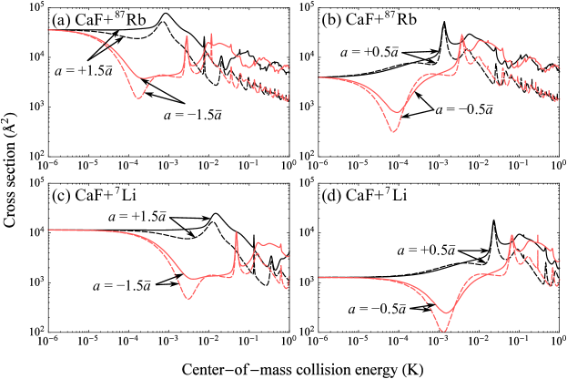
Figure 1: (Color online) Total elastic cross section, $\sigma_{\text{el}}$ (solid lines), and transport cross section, $\sigma_{\eta}^{(1)}$ (dashed lines), for positive (black) and negative (red/gray) signs of the scattering length. (a) CaF+⁸⁷Rb, $\left|a\right|=1.5\bar{a}$; (b) CaF+⁸⁷Rb, $\left|a\right|=0.5\bar{a}$; (c) CaF+⁷Li, $\left|a\right|=1.5\bar{a}$; (d) CaF+⁷Li, $\left|a\right|=0.5\bar{a}$.

Exact scattering calculations on systems as complex as Li+CaF and Rb+CaF are not currently feasible. The combination of a deep chemical well, very large anisotropy of the interaction potential, and small CaF rotational constant mean that a very large rotational basis set would be needed for convergence. In addition, even if converged results could be achieved, uncertainties in the potential surface mean that no single calculation could be taken to represent the true system and many calculations on many surfaces would be needed to explore the range of possible behaviors Cvitaš et al. (2007). Instead we model the interactions with a simple single-channel model potential which we choose to be the Lennard-Jones potential, $V(r)=-C_{6}/r^{6}+C_{12}/r^{12}$, where $r$ is the intermolecular distance. We have shown previously Frye et al. (2015) that, while a simple single-channel model cannot be expected to reproduce a full coupled-channel calculation, it can quantitatively reproduce the range of behaviors shown by full calculations.

We obtain Lennard-Jones parameters for Li+CaF from ab initio calculations Morita and Hutson (2015). We obtain $C_{6\rm,Li+CaF}=1767\,E_{\rm h}a_{0}^{6}$ from direct fitting to the isotropic part of the long-range potential, where $E_{\rm h}$ is the Hartree energy and $a_{0}$ is the Bohr radius. We set $C_{12\rm,Li+CaF}=2.37\times 10^{7}\,E_{\rm h}a_{0}^{12}$ to reproduce the depth of the complete potential, which is 7224 cm^-1. We use the depth of the complete potential in preference to the depth of the isotropic part of the potential because the very large anisotropy at short-range means the isotropic part of the potential is not representative of the interaction. To obtain a $C_{6}$ parameter for Rb +CaF we first separate $C_{6\rm,Li+CaF}$ into induction and dispersion contributions. Induction contributions for both systems are readily calculated from known values of the CaF dipole moment Childs et al. (1984) and the static polarizabilities of the atoms Derevianko et al. (2010). The dispersion contribution for Rb+CaF can then be calculated from the dispersion contribution for Li+CaF using Tang’s combining rule Tang (1969) with known homonuclear diatomic dispersion coefficients Derevianko et al. (2010), atomic polarizabilities Derevianko et al. (2010) and a calculated CaF polarizability of $\alpha_{\rm CaF}=137a_{0}^{3}$. The sum of these contributions gives $C_{6\rm,Rb+CaF}=3084\,E_{\rm h}a_{0}^{6}$. We estimate, by analogy to calculations on methyl fluoride Lutz and Hutson (2014), that the well depth for Rb+CaF will be about 2.5 times shallower than for Li+CaF. This sets $C_{12\rm,Rb+CaF}=1.8\times 10^{8}\,E_{\rm h}a_{0}^{12}$.

For our purposes, the key property of a potential is the s-wave scattering length, $a$, that it produces. In the present work, we vary the $C_{12}$ coefficient over a small range (with $C_{6}$ fixed) to vary the scattering length. We focus on four typical scattering lengths, $a=-1.5\bar{a}$, $-0.5\bar{a}$, $+0.5\bar{a}$, $+1.5\bar{a}$, where $\bar{a}$ is the mean scattering length of Gribakin and Flambaum Gribakin and Flambaum (1993), $\bar{a}=20.2$ Å for Li+CaF and $35.7$ Å for Rb+CaF.

Discussions of thermalization have usually assumed that the relevant cross section is the elastic cross section $\sigma_{\rm el}$, which is the unweighted integral of the differential cross section $d\sigma/d\omega$,

$$\sigma_{\rm el}=2\pi\int\frac{d\sigma}{d\omega}\sin\Theta\,d\Theta,$$ (1)

where $d\omega$ is an element of solid angle and $\Theta$ is the deflection angle in the center-of-mass frame. However, small-angle scattering contributes fully to $\sigma_{\rm el}$ but contributes relatively little to thermalization. The transport cross section that takes proper account of this is $\sigma_{\eta}^{(1)}$ Frye and Hutson (2014),

$$\sigma_{\eta}^{(1)}=2\pi\int\frac{d\sigma}{d\omega}(1-\cos\Theta)\sin\Theta\,d\Theta.$$ (2)

In the present work, scattering calculations are carried out using the MOLSCAT package Hutson and Green (1994). We use the DCS post-processor Green and Hutson (1996) to calculate differential cross sections, and the SBE post-processor Hutson and Green (1982) to calculate $\sigma_{\eta}^{(1)}$.

The calculated elastic and transport cross sections for Li+CaF and Rb+CaF are shown in Fig. 1 for a variety of scattering lengths. At low energy, in the s-wave regime, the cross sections have constant limiting values of $4\pi|a|^{2}$. This is the same for both $\sigma_{\rm el}$ and $\sigma_{\eta}^{(1)}$, because pure s-wave scattering is isotropic. The cross sections for positive and negative scattering lengths go to the same low-energy limit. However, as energy increases, the cross sections all diverge from one another. Those for negative scattering lengths, especially $a=-0.5\bar{a}$, show dramatic Ramsauer-Townsend minima as the scattering phase shift, and hence the s-wave cross section, passes through a zero Child (1974). For $\sigma_{\eta}^{(1)}$ this minimum is further deepened by destructive interference between s-wave and p-wave scattering Frye and Hutson (2014). For $a=+1.5\bar{a}$ a peak in both cross sections is seen (near $~{}10^{-3}$ K for Rb+CaF). This is a d-wave feature corresponding to the energy of the centrifugal barrier maximum. At higher energies, there are various shape resonances present for all cases. Nevertheless, once many partial waves contribute, the cross sections become less dependent on scattering length and approach classical limits.

It may be noted that the cross sections for the two systems for the same value of $a/\bar{a}$ are very similar, apart from constant factors in energy and cross section. In fact they would be nearly identical if the cross sections were in units of $\bar{a}^{2}$ and energy in units of $\bar{E}=\hbar^{2}/(2\mu\bar{a}^{2})$ Frye and Hutson (2014); Gao (2001), where $\bar{E}=9.51$ mK for Li+CaF and $0.543$ mK for Rb+CaF. This scaling means that, while the Rb+CaF cross sections are almost independent of scattering length at 10 mK and above, the Li+CaF cross sections are highly sensitive to scattering length at any energy below 100 mK.

For stationary atoms the molecular kinetic energy in the laboratory frame, $E^{\text{lab}}_{\text{CaF}}$, is related to the collision energy in the center-of-mass frame, $E^{\text{CM}}$, by $E^{\text{lab}}_{\text{CaF}}=(m_{\text{CaF}}/\mu)E^{\text{CM}}$, where $\mu=m_{\text{CaF}}m_{\text{at}}/(m_{\text{CaF}}+m_{\text{at}})$ is the reduced mass of the collision system, $m_{\text{CaF}}$ is the molecular mass and $m_{\text{at}}$ is the atom mass. The ratio $E^{\text{lab}}_{\text{CaF}}/E^{\text{CM}}$ is 9.40 for Li+CaF and 1.68 for Rb+CaF. This introduces a further energy scaling between the two systems in addition to the difference in $\bar{E}$.

Because the molecules are in the ground state, and the rotational excitation energy is far greater than the available collision energy, we assume that there are no inelastic collisions. It is known that there can be molecule-molecule inelastic collisions in the presence of the microwave field, even when the microwave frequency is well below the first rotational resonance Kajita and Avdeenkov (2007); Avdeenkov (2009). This is a concern for evaporative cooling of molecules, but less so for sympathetic cooling, where the density of molecules can be low. It is worth studying whether there can be atom-molecule inelastic collisions induced by the microwave field, but that is beyond the scope of this paper.

III Simulation method

We assume that ground state CaF molecules are confined around the central antinode of a standing-wave microwave field, formed at the center of an open microwave cavity Dunseith et al. (2015). The interaction potential of the molecules with the microwave field is

$$U({\bf r})=-\Delta U\exp\left[-\frac{x^{2}}{w_{x}^{2}}-\frac{y^{2}}{w_{y}^{2}}\right]\cos^{2}\left(\frac{2\pi z}{\lambda}\right),$$ (3)

where $\Delta U$ is the trap depth and we take $\Delta U/k_{\text{B}}=400$ mK, $w_{x}=16.3$ mm, $w_{y}=15.3$ mm, and $\lambda=21.3$ mm Dunseith et al. (2015). The initial phase-space distribution of the molecules is assumed to be

$$f({\bf r},{\bf p}) = \frac{n_{0,\text{CaF}}}{(2\pi m_{\rm CaF}k_{\text{B}}T)^{3/2}}$$ (4)

$$\times \exp\left[-\frac{U({\bf r})-U(0)\!+p^{2}/(2m_{\rm CaF})}{k_{\text{B}}T}\right],$$

where $T$ is the initial temperature of the molecules and $n_{0,\text{CaF}}$ is the initial density at the center of the trap, which is fixed such that the total number of molecules is $N_{\text{CaF}}=10^{5}$. For most simulations, we take $T=70$ mK in order to study sympathetic cooling from a high temperature. A distribution of ultracold atoms is overlapped with the molecules. The atoms are in a harmonic magnetic trap whose depth is 1 mK. We assume that the distribution of atoms in phase space depends only on their energy. Therefore, at all times, the atoms have a Gaussian spatial distribution and a thermal velocity distribution with temperature $T_{\text{at}}$. They have an initial temperature of 100 $\mu$K, an initial central density of $10^{11}$ cm^-3, and an initial number of $10^{9}$. The corresponding initial $1/e$ radius is 1.2 mm. This initial temperature and density can be reached by first collecting and cooling the atoms in a magneto-optical trap, followed by a brief period of sub-Doppler cooling in a molasses before loading into the magnetic trap. For Rb, polarization gradient cooling is an effective sub-Doppler cooling mechanism, while for Li velocity-selective coherent population trapping in a gray molasses can be used Grier et al. (2013); Burchianti et al. (2014). Our approximation that the molecules are confined only by the microwave field, and the atoms only by the magnetic field, is a reasonable one, though our model could be extended to use the complete potential of both species in the combined fields.

For each molecule, the simulation proceeds as follows. We solve the equation of motion in the microwave trap for a time step $\Delta t$ which is much smaller than the mean time between collisions. Then, using the current position, ${\bf r}$ and velocity, ${\bf v}$, of the molecule, we determine whether or not there should be a collision as follows. The velocity of an atom is chosen at random from a thermal distribution with temperature $T_{\text{at}}$. From the atomic and molecular velocities we calculate the collision energy in the center-of-mass frame, $E^{\text{CM}}$. The collision probability is $P=n_{\text{at}}({\bf r})\sigma(E^{\text{CM}})v_{\text{r}}\Delta t$, where $v_{\text{r}}$ is the relative speed of the atom and molecule, $n_{\text{at}}$ is the atomic density, and $\sigma(E^{\text{CM}})$ is either $\sigma_{\text{el}}$ or $\sigma_{\eta}^{(1)}$ (see Sec. IV). A random number is generated in the interval from 0 to 1, and if this is less than $P$ a collision occurs. If there is no collision, the velocity of the molecule is unchanged. If there is a collision, the velocities are transformed into the center-of-mass frame, a deflection angle is determined as described below, and the new velocities transformed back into the laboratory frame. If the new total energy (kinetic energy plus trapping potential) is sufficient for the atom to escape from the trap, the atom, and its energy prior to the collision, are removed. The change in energy is shared among all the remaining atoms. Otherwise, the atom remains in the trap and the change in kinetic energy is shared between all the atoms. This algorithm is followed for each molecule in the distribution. The density and temperature of the atom cloud are updated to account for the atom loss and atom heating at this time step, and then the simulation proceeds to the next time step.

With our choice of trap depth and initial atom temperature, there is a small evaporative cooling effect due to atom-atom collisions. For Rb, over the 50 s timescale of our simulations, 8% of the atoms are lost and the temperature falls to $80\,\mu$K. Prior to Sec. IX, we neglect this evaporative cooling effect in our simulations because we wish to isolate effects that are due to atom-molecule collisions. Then, in Sec. IX, we include atom-atom collisions and explore the effects of evaporative cooling.

As we will see, the molecular velocity distributions obtained during the cooling process are far from thermal. There are some molecules that never have a collision during the whole simulation and so remain at high energy throughout. Almost all these molecules have a kinetic energy greater than 10 mK, and they disproportionately skew the mean kinetic energy of the sample as a whole. Our interest is in the molecules that cool, and so we separate the kinetic energy distribution into two parts, above and below 10 mK. To express how well the cooling works, we give the fraction of molecules in the low-energy part, and their mean kinetic energy, both as functions of time.

IV Collision models

In previous modeling Tokunaga et al. (2011), atoms and molecules collided like hard spheres. In this model, the momenta in the center-of-mass frame before and after a collision, ${\bf p}_{\text{c}}$ and ${\bf p}_{\text{c}}^{\prime}$, are related by

$${\bf p}_{\text{c}}^{\prime}={\bf p}_{\text{c}}-2({\bf p}_{\text{c}}\cdot{\bf\hat{e}}){\bf\hat{e}},$$ (5)

where ${\bf\hat{e}}$ is a unit vector along the line joining the centers of the spheres, given by

$${\bf\hat{e}}={\bf\hat{p}}_{\text{c}}\sqrt{1-|{\bf b}|^{2}}+{\bf b},$$ (6)

where ${\bf\hat{p}}_{\text{c}}$ is a unit vector in the direction of ${\bf p}_{\text{c}}$ and ${\bf b}$ is a vector that lies in a plane perpendicular to ${\bf p}_{\text{c}}$ and whose magnitude is the impact parameter divided by the sum of the radii of the two spheres. For each collision, ${\bf b}$ is chosen at random from a uniform distribution, subject to the constraints ${\bf b}\cdot{\bf p}_{\text{c}}=0$ and $|{\bf b}|\leq 1$.

Figure 2: (Color online) Results of various collision models: (i) hard-sphere model with energy-independent cross section $4\pi\bar{a}^{2}$; (ii) full energy-dependent differential cross section model; (iii) hard-sphere model with $\sigma_{\text{el}}(E^{\text{CM}})$; (iv) hard-sphere model with $\sigma_{\eta}^{(1)}(E^{\text{CM}})$; (v) hard-sphere model with classical approximation to $\sigma_{\eta}^{(1)}(E^{\text{CM}})$. The graphs show: (a) Cross section versus collision energy; (b) fraction of molecules with kinetic energy below 10 mK versus time; (c) mean kinetic energy of that fraction versus time. The coolant is Rb and $a=+1.5\bar{a}$.

The lines labeled (i) in Fig. 2 show how the cooling proceeds for CaF + Rb when we use the hard-sphere model and choose the cross section to be independent of energy and equal to $4\pi\bar{a}^{2}=1.59\times 10^{-16}$ m². The cross section is shown in Fig. 2(a), while the cold fraction and the mean kinetic energy of that fraction are shown in parts (b) and (c), both as functions of time. As explained in Sec. III, the cold fraction is defined as the fraction with kinetic energy below 10 mK. The cold fraction increases rapidly, and that fraction thermalizes quickly with the atoms. After just 4 s, 85% of the molecules are in the cold fraction and their mean energy is within 50% of the 100 $\mu$K temperature of the coolant atoms.

The energy-independent hard-sphere (EIHS) model described above is reasonable at very low energy, but it has three deficiencies. First, it neglects the fact that the low-energy cross sections are actually $4\pi a^{2}$, where $a$ is the true scattering length as opposed to the mean scattering length. The true scattering length can take any value between $-\infty$ and $+\infty$, but is generally unknown for a specific system until detailed measurements are available to determine it. Secondly, the EIHS model neglects the fact that real cross sections are strongly energy-dependent, usually showing resonance structure on a background that drops off sharply with increasing energy, as shown in Fig. 2(a). Thirdly, collisions with small deflection angles (forwards scattering) do not contribute efficiently to cooling, and the EIHS model neglects the fact that differential cross sections (DCS) at higher energies tend to be dominated by such forwards scattering, because many collisions encounter only the attractive long-range tail of the interaction potential.

To remedy all these deficiencies, we introduce here a new model that we call the full DCS model. For this we calculate realistic integral and differential cross sections, as described above, for a variety of choices of the scattering length $a$. We use the elastic cross section $\sigma_{\text{el}}(E^{\text{CM}})$ from these calculations to determine the collision probability. This cross section is curve (ii) in Fig. 2(a), and it is smaller than in the EIHS model at collision energies above 8 mK, but larger below 8 mK. We then select a deflection angle $\Theta$ from a random distribution that reproduces the full differential cross section, $d\sigma/d\omega$, at energy $E^{\text{CM}}$. To select a deflection angle at random from this distribution, we form the cumulative distribution function,

$$S(\Theta)=\frac{2\pi}{\sigma_{\text{el}}}\int_{0}^{\Theta}\frac{d\sigma}{d\omega}\sin(\Theta^{\prime})d\Theta^{\prime},$$ (7)

select a random number $r$ between 0 and 1, and find the value of $\Theta$ where $S(\Theta)=r$.

The full DCS model is our most complete one and we have used it for all the simulations in the following sections. Its results for the choice $a=+1.5\bar{a}$ are shown by the lines labeled (ii) in Fig. 2. It may be seen that the cooling proceeds more slowly than in the EIHS model. It takes 14 s for the cold fraction to reach 80% and for the energy of that fraction to be within 50% of the temperature of the atoms. The slower cooling is mainly due to the dominance of forward scattering at higher energies.

There are three approximations to the full-DCS model that are worth considering because they avoid the tabulation of differential cross sections and cumulative distributions. The first of these is to use a hard-sphere collision model but to take the full energy-dependent elastic cross section from Fig. 2(a). This produces the cooling behavior labeled (iii) in Figs. 2(b) and (c). It may be seen that this model produces cooling slightly slower than the EIHS model, but considerably faster than the full DCS model. The second and more satisfactory approximation is to use a hard-sphere collision model but to take the full energy-dependent transport cross section $\sigma_{\eta}^{(1)}$, shown as line (iv) in Fig. 2(a). We label this approach EDT-HS. It produces the cooling behavior labeled (iv) in Figs. 2(b) and (c). It may be seen that it models the cooling of the molecules very accurately, because it takes proper account of the reduced efficiency of small-angle collisions for sympathetic cooling. However, as will be seen in Sec. VIII, the EDT-HS approach does not adequately model heating and loss of the coolant atoms.

It is worth exploring whether a classical calculation of $\sigma_{\eta}^{(1)}$ would suffice. Unlike the elastic cross section, $\sigma_{\eta{\rm,class}}^{(1)}$ is finite because the factor of $1-\cos\Theta$ suppresses the divergence due to forwards scattering. We have calculated $\sigma_{\eta{\rm,class}}^{(1)}$ for the Lennard-Jones potentials described above,

$$\sigma_{\eta{\rm,class}}^{(1)}=2\pi\int_{0}^{\infty}b[1-\cos\Theta(b)]db,$$ (8)

where $b$ is the impact parameter and $\Theta(b)$ is the classical deflection function Child (1974). We find that it is very well approximated by the power law $\sigma_{\eta}^{(1)}(E^{\text{CM}})=A(E^{\text{CM}}/C_{6})^{-1/3}$, with the dimensionless constant $A=4.79$. This cross section is labeled (v) in Fig. 2(a). It agrees well with the quantum-mechanical $\sigma_{\eta}^{(1)}(E^{\text{CM}})$ for Rb+CaF at high energies, as we would expect when many partial waves contribute. Remarkably, the temperature and cold fraction shown for this model in Fig. 2 agree very well with those for model (ii), even as the temperature approaches 100 $\mu$K. This is an atypical result because, for $a=+1.5\bar{a}$, $\sigma_{\eta{\rm,class}}^{(1)}$ is within a factor of about three of the quantum-mechanical $\sigma_{\eta}^{(1)}$ at all energies above 3 $\mu$K. For other values of $a$, the two cross sections can differ by more than a factor of three at energies below about $2\bar{E}$, which is around 1 mK for Rb+CaF. Note that the classical approximation will be less successful for a lighter coolant such as Li where $\bar{E}$ is far higher.

V Approximate cooling rates

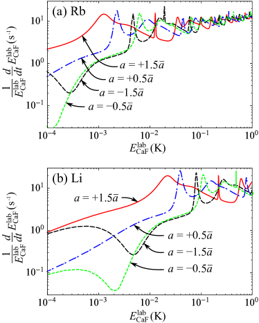
Figure 3: (Color online) Cooling rate of molecules as a function of their kinetic energy, estimated from Eq. (9), when the coolant is (a) Rb and (b) Li, and for various values of the s-wave scattering length: $a=+1.5\bar{a}$ (red solid line), $a=+0.5\bar{a}$ (blue dash-dot line), $a=-0.5\bar{a}$ (green dotted line), and $a=-1.5\bar{a}$ (black dashed line).

From the transport cross sections, $\sigma^{(1)}_{\eta}$, in Fig. 1 we can make a useful estimate of the cooling rate of molecules as a function of their kinetic energy. For this estimate, we assume stationary atoms with a uniform density $n_{\text{at}}=10^{11}$ cm^-3. The cooling rate is

$$\frac{d{E^{\text{lab}}_{\text{CaF}}}}{dt}={n_{\text{at}}}{\sigma}(E^{\text{CM}})v\overline{{\Delta}E},$$ (9)

where $v=(2E^{\text{lab}}_{\text{CaF}}/m_{\text{CaF}})^{1/2}$ is the speed of the molecule and $\overline{{\Delta}E}$ is the average energy transfer for a hard-sphere collision. $\Delta E$ is given explicitly as

$$\Delta E=-\left(\frac{2\mu}{m_{\rm CaF}+m_{\rm at}}\right)(1-\cos\Theta)E^{\text{lab}}_{\text{CaF}}.$$ (10)

Figure 3 shows the cooling rates obtained this way, which although only approximate are helpful for understanding the numerical results presented later. For collisions with Rb at energies above 10 mK, the cooling rate does not depend strongly on the s-wave scattering length. This is the energy regime where the $a$-independent classical approximation to $\sigma_{\eta}^{(1)}(E^{\text{CM}})$ described in Sec. IV is accurate. Due to the small reduced mass in the lithium case, the classical limit is only reached for temperatures above 200 mK, and so the cooling rate depends sensitively on $a$ over the whole energy range of interest. When $a$ is negative there is a minimum in the cooling rates corresponding to the Ramsauer-Townsend minimum in $\sigma_{\eta}^{(1)}(E^{\text{CM}})$. For Rb, at $a=-1.5\bar{a}$, this minimum is near 100 $\mu$K, which is close to the temperature of the atoms in our simulations and so will not have a significant impact on the thermalization. For Li, the minimum occurs for kinetic energies between 1 and 10 mK, and so it has a strong effect on the thermalization. Finally, we note that in the ultracold limit the cooling rate is almost an order of magnitude higher for Rb than for Li, reflecting the larger value of $\bar{a}$ for Rb + CaF relative to Li + CaF.

VI Cooling dynamics

Figure 4: (Color online) Time evolution of the phase-space distribution of molecules in the $x$ direction. The cooling times are (a) 0 s, (b) 2 s, (c) 10 s, and (d) 20 s. The coolant is Rb and $a=+1.5\bar{a}$.

Figure 4 shows the evolution of the $(x,v_{x})$ phase-space distribution of CaF when Rb atoms are used as the coolant, for the case where the s-wave scattering length is $a=+1.5\bar{a}$. At $t=0$ (Fig. 4(a)), the molecules fill the phase-space acceptance of the trap. At later times, more and more molecules congregate at the trap center as they are cooled by collisions with the atoms. After 20 s (Fig. 4(d)), the distribution has separated into two parts. The majority are cooled to the center, but there are some that remain uncooled. These are molecules that have large angular momentum around the trap center and so are unable to reach the center where the atomic density is high. At $x=3$ mm for example, the atomic density, and hence the collision rate, is a factor of 1000 smaller than at the center, and so molecules at this distance are unlikely to collide with atoms on the 20 s timescale shown in the figure. These molecules can be cooled by expanding the size of the atom cloud, but only at the expense of the overall cooling rate Tokunaga et al. (2011).

Figure 5: (Color online) Kinetic energy distributions after 2 s, 10 s, and 20 s. The coolant is Rb. Left panels have $a=+1.5\bar{a}$ while right panels have $a=-1.5\bar{a}$.

Figure 5(a) shows histograms of the kinetic energy distribution of the molecules at three different times, 2, 10 and 20 s, when the coolant is Rb and $a=+1.5\bar{a}$. These are the same times as chosen for the phase space distributions in Fig. 4, and the results come from the same simulation. The initial distribution is a Maxwell-Boltzmann distribution with a temperature of 70 mK, truncated at the trap depth of 400 mK. The distribution rapidly separates into two parts, those that cool and those that do not. The latter are the molecules that never reach the trap center because of their large angular momentum, as discussed above. A significant fraction of molecules are cooled below 1 mK after just 2 s. After 10 s the majority are in this group, and after 20 s this cold fraction is almost fully thermalized with the atoms. We return to part (b) of Fig. 5 in the next section.

VII Sensitivity to the scattering length and the choice of coolant

At low energies, cross sections are very sensitive to the exact form of the scattering potential, as shown in Fig. 1, and cannot be calculated accurately without independent knowledge of the scattering length. In our model Lennard-Jones potential, the full energy-dependence of the cross section is determined once the s-wave scattering length, $a$, is fixed. Here, we study how the simulation results change as we vary the value of $a$. The choice of coolant is also a crucial consideration, and so we compare the results for Li and Rb as coolants.

VII.1 Evolution of the kinetic energy distributions

Figure 5 compares how the kinetic energy distributions evolve for two cases: $a=+1.5\bar{a}$ and $a=-1.5\bar{a}$, with Rb as the coolant. At 2 s the two distributions are similar. The main difference is that the distribution extends to lower energies for $a=+1.5\bar{a}$. The similarity is due to the similar cooling rates at the high energies, as shown in Fig. 3(a), while the difference at low energy is due to the far higher cooling rate for $a=+1.5\bar{a}$ at energies below 1 mK (compare the solid red and black dashed lines in Fig. 3(a)). Exactly the same trend is seen after 10 s of cooling. Once again, the high-energy parts of the distributions are very similar, but the distribution extends to lower energies for the $a=+1.5\bar{a}$ case. After 20 s the majority of the molecules have fully thermalized with the atoms and the two distributions are very similar to one another.

Figure 6 shows the corresponding histograms for the case of Li. Here, the cooling proceeds more slowly and so we have added a fourth pair of histograms showing the distributions after 40 s. There is a great contrast between the positive and negative scattering lengths in this case. For $a=+1.5\bar{a}$ the distribution evolves in a very similar manner to the Rb case, but when $a=-1.5\bar{a}$ it takes a long time for the molecules to reach energies below 10 mK. This is the effect of the Ramsauer-Townsend minimum which reduces the cooling rate estimated in Fig. 3(b) to 0.25 s^-1 for kinetic energies near 20 mK. Because the minimum is broad in energy, and there is a large mass mismatch between CaF and Li, a collision cannot take a molecule directly across the minimum. The molecules have to be cooled through the minimum by multiple collisions, and that takes a long time. Once molecules have passed through this minimum, cooling to ultracold temperatures occurs on a similar timescale to the $a=+1.5\bar{a}$ case.

Figure 6: (Color online) Kinetic energy distributions after 2 s, 10 s, 20 s and 40 s. The coolant is Li. Left panels have $a=+1.5\bar{a}$ while right panels have $a=-1.5\bar{a}$.

VII.2 Cold fraction and mean kinetic energy

Figure 7: (Color online) Fraction of molecules with kinetic energy below 10 mK as a function of time for (a) Rb, and (b) Li, for four different values of the scattering lengths: $a=+1.5\bar{a}$ (red), $a=+0.5\bar{a}$ (blue), $a=-0.5\bar{a}$ (green), and $a=-1.5\bar{a}$ (black).

Figure 7(a) shows the fraction of molecules with kinetic energy less than 10 mK, as a function of time, for various values of $a$ when the coolant is Rb. This fraction is entirely insensitive to $a$. This is because the cooling rate is independent of $a$ for energies above 10 mK, as we saw in Fig. 3. After 5 s about 50% of the molecules are in this cold fraction, and after 20 s this exceeds 80%. Figure 7(b) shows the cold fraction versus time when the coolant is Li. We find a strong dependence on $a$ in this case. When $a=+1.5\bar{a}$, the increase in the cold fraction with time is similar to the Rb case. For this value of $a$ there is a maximum in the cooling rate at a kinetic energy of about 70 mK (see Fig. 3(b)), which happens to match the initial temperature of the molecules, and so the cooling to below 10 mK proceeds rapidly. The cold fraction reaches 50% after 4 s in this case. The increase in the cold fraction is slower for $a=+0.5\bar{a}$, reaching 50% after 16 s. The accumulation of cold molecules is exceedingly slow when $a$ is negative. When $a=-1.5\bar{a}$, the Ramsauer-Townsend minimum is at $E^{\text{lab}}_{\text{CaF}}=20$ mK, and it takes a long time for the molecules to cool through this minimum. The cold fraction reaches 50% after 40 s in this case. When $a=-0.5\bar{a}$, the Ramsauer-Townsend minimum is shifted to $E^{\text{lab}}_{\text{CaF}}=10$ mK, but the cross section at the minimum is a factor of five smaller, and so the cooling is even slower, taking 50 s to reach 50%.

Figure 8: (Color online) Mean kinetic energy of the cold fraction as a function of time when the coolant is (a) Rb and (b) Li, and for various values of the s-wave scattering length: $a=+1.5\bar{a}$ (red), $a=+0.5\bar{a}$ (blue), $a=-0.5\bar{a}$ (green), and $a=-1.5\bar{a}$ (black).

Figure 8(a) shows the mean kinetic energy of the cold fraction as a function of time for various values of $a$ when Rb is used as the coolant. As for the cold fraction itself, this measure is almost independent of $a$. This may seem surprising, since the cooling rates estimated in Fig. 3(a) show a strong dependence on $a$ below a few mK. However, the mean kinetic energy is strongly influenced by molecules with kinetic energies close to the 10 mK cutoff that defines the cold fraction, and at this energy the cooling rates show little dependence on $a$. We find a small difference in the cooling rates between positive and negative scattering lengths. For the positive $a$ values the molecular temperature is within a factor of two of the atomic temperature after 10 s, while for the negative $a$ values this takes 14 s. Figure 8(b) shows how the mean kinetic energy of the cold fraction evolves when Li is used as a coolant. In this case, the cooling depends sensitively on $a$. When $a=+1.5\bar{a}$ the evolution is similar to the Rb case. The cooling is much slower when $a=+0.5\bar{a}$ because the low-energy cross-section is nine times smaller. The cooling is even slower when $a$ is negative. This is because, in the energy region between 1 and 10 mK, the Ramsauer-Townsend minimum greatly suppresses the cooling rate relative to the positive $a$ case, and because molecules with energies in this range have a strong influence on the mean.

The fraction of molecules that are cooled below 10 mK depends on the initial temperature, $T_{\text{i}}$. Figure 9 compares this fraction for $T_{\text{i}}=20$ mK and 70 mK, for the case where Rb is the coolant and $a=+1.5\bar{a}$. These two initial temperatures correspond to temperatures of 2 mK and 30 mK prior to compression of the cloud in the microwave trap. When $T_{\text{i}}=20$ mK, more than 99% of the molecules are cold within 10 s.

Figure 9: (Color online) Fraction of cold molecules as a function of time for the initial temperatures of $T_{\text{i}}=20$ mK (red solid line), and $T_{\text{i}}=70$ mK (black dashed line). The coolant is Rb and $a=+1.5\bar{a}$.

VIII Atom heating and loss

Figure 10: (a) Atom heating rate per molecule and (b) atom loss rate per molecule for the EDT-HS model (dashed line) and the full DCS model (solid line). The coolant is Rb, $a=+1.5\bar{a}$, and the molecules have an initial temperature of 70 mK. There are $10^{5}$ molecules and $10^{9}$ atoms.

The energy transferred from molecules to atoms will either eject atoms from the trap, or will heat them up. As described in Sec. III, we suppose that atoms are lost from the trap if their total energy exceeds 1 mK. This could be the actual depth of the trap, or an “rf knife” might be used to cut off the trap at this depth. Here, we investigate the heating and loss of atoms and the consequences for sympathetic cooling. We note that while the EDT-HS collision model correctly captures the molecule cooling dynamics when $\sigma_{\eta}^{(1)}$ is used as the cross section, it does not model correctly the atom heating and loss. Here, we highlight the difference between these two approaches by comparing the results obtained from the EDT-HS model and the full DCS model.

Figure 10 shows how the heating and loss rates of the atoms change with time in the full DCS model and the EDT-HS model for the case of $10^{5}$ molecules and $10^{9}$ atoms. The two models show similar trends, so we first discuss these trends and then consider the differences between the models. At early times the majority of the molecules have energies far above the atom trap depth and so most collisions cause atom loss, rather than heating. The loss rate is high while the heating rate is low. Nevertheless, there is still some heating due to small-angle collisions with the molecules which transfer only a little energy to the atoms. The loss rate increases during the first second because the collision cross section and the atom-molecule overlap both increase as the molecules are cooled. As time goes on the loss rate falls because the molecules are cooler and there are fewer collisions with enough energy to kick atoms out of the trap. For the same reason the heating rate initially increases, but then decreases again as the molecules have less energy to transfer to the atoms. For most of the 20 s period, the full DCS model gives more atom heating and more atom loss than the EDT-HS model. Only at long times, once the atoms and molecules are almost fully thermalized, do the two models give the same results.

Integrating the results of the full DCS model shown in Fig. 10, we find that the total temperature increase of the trapped atoms is 1.3 pK per molecule, while the total loss is 10 atoms per molecule. The energy deposited into the trapped atom cloud is only 1.8% of the initial energy of the molecular cloud. In this sense, the sympathetic cooling process is remarkably efficient.

We now turn to how the atom heating and loss rates can be understood, and explain why the two models give different results. Whether an atom is heated or lost depends on the kinetic energy kick it receives in the collision, as given by Eq. (10) if the atoms are assumed to be stationary. An atom at the center of the trap is lost from the trap if the energy transferred in the collision exceeds the trap depth, $\Delta E>E_{\text{trap}}$. This occurs if the deflection angle exceeds a critical angle $\Theta_{\text{crit}}$ given by

$$\cos\Theta_{\text{crit}}=1-\left(\frac{m_{\rm CaF}+m_{\rm at}}{2\mu}\right)\left(\frac{E_{\text{trap}}}{E^{\text{lab}}_{\text{CaF}}}\right).$$ (11)

At laboratory-frame energies below critical energy $E_{\rm crit}=(m_{\rm CaF}+m_{\rm at})/4\mu)E_{\text{trap}}$, no loss is possible, assuming stationary atoms at the center of the trap. This energy is 2.63 mK for Li+CaF and 1.04 mK for Rb+CaF. All collisions below this energy and collisions above this energy where $\Theta<\Theta_{\text{crit}}$ will not eject atoms from the trap, but still transfer energy and so heat the atom cloud, by an amount proportional to $1-\cos\Theta$. This suggests the possibility of defining cross sections for atom heating and loss as partial integrals of the differential cross section,

$$\sigma_{\text{loss}}=2\pi\int_{-1}^{\cos\Theta_{\text{crit}}}\frac{d\sigma}{d\omega}d\cos\Theta,\\$$ (12)

$$\sigma_{\text{heat}}=2\pi\int_{\cos\Theta_{\text{crit}}}^{1}\frac{d\sigma}{d\omega}(1-\cos\Theta)d\cos\Theta.$$ (13)

It is convenient to write these as integrals over $d\cos\Theta$ instead of $\sin\Theta\,d\Theta$ because the $\cos\Theta$ form allows us to show plots in which the integrals are simply areas that can be estimated by eye. Note that if $E^{\text{lab}}_{\text{CaF}}<E_{\rm crit}$ then $\sigma_{\text{heat}}=\sigma_{\eta}^{(1)}$, because all collisions cause heating rather than loss. For the full DCS model these integrals must be evaluated numerically, but in the hard-sphere model the DCS are isotropic, $d\sigma_{\rm HS}/d\omega=\sigma_{\rm HS}/(4\pi)$, and the integrals can be evaluated analytically to give

$$\sigma_{\rm loss,HS}=\frac{1}{2}(1+\cos\Theta_{\rm crit})\sigma_{\rm HS}$$ (14)

and

$$\sigma_{\rm heat,HS}=\frac{1}{4}(1-\cos\Theta_{\rm crit})^{2}\sigma_{\rm HS}.$$ (15)

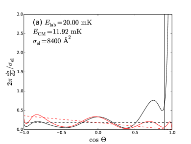
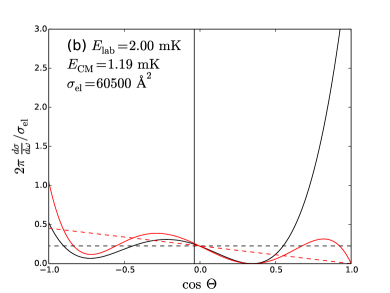
Figure 11: (Color online) Differential cross sections and their contributions to heating and loss. The solid black line shows the full quantum-mechanical $d\sigma/d\omega$, while the solid red line shows $(1-\cos\Theta)d\sigma/d\omega$; the dashed lines show the corresponding quantities for the EDT-HS model. The vertical line shows the value of $\Theta_{\text{crit}}$. (a) $E^{\text{lab}}_{\text{CaF}}=2$ mK. (b) $E^{\text{lab}}_{\text{CaF}}=20$ mK. The coolant is Rb and $a=+1.5\bar{a}$.

Figure 11 shows differential cross sections at two energies that correspond to $E^{\text{lab}}_{\text{CaF}}=2$ mK and 20 mK for Rb+CaF. Both full differential cross sections and those from the EDT-HS model are shown (solid and dashed black lines respectively), and the corresponding quantities weighted by $1-\cos\Theta$ are shown in red. The values of $\Theta_{\rm crit}$ at the two energies are shown as vertical lines. Integrals over the complete range of $\cos\Theta$ under the black lines correspond to $\sigma_{\rm el}$, and under red lines correspond to $\sigma_{\eta}^{(1)}$; the latter is the same for the full DCS and EDT-HS models by construction. $\sigma_{\rm loss}$ is the area under the black lines to the left of $\Theta_{\rm crit}$, and $\sigma_{\rm heat}$ is the area under the red lines to the right of $\Theta_{\rm crit}$. It can be seen that at 20 mK the full DCS has a very large forwards peak; this dominates $\sigma_{\rm heat}$, even though its contribution is suppressed by the $1-\cos\Theta$ weighting. The resulting $\sigma_{\rm heat}$ is many times larger than in the EDT-HS model, which has no forward peak. The full DCS also has a secondary peak near $\cos\Theta=0.75$, which is outside $\Theta_{\rm crit}$ and so contributes to atom loss; the resulting $\sigma_{\rm loss}$ is also larger than in the EDT-HS model. At the lower energy of 2 mK, $\Theta_{\rm crit}$ is near $\Theta=\pi/2$. There is still a large forwards peak but it no longer dominates due to the changed range of integration, leading to similar cross sections for the two models.

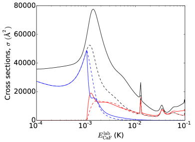
Figure 12: (Color online) Loss (red) and heating (blue) cross sections as a function of CaF laboratory energy for the EDT-HS model (dashed lines) and the full DCS model (solid lines). $\sigma_{\text{el}}$ (solid black line) and $\sigma_{\eta}^{(1)}$ (dashed black line) are shown for comparison. The coolant is Rb and $a=+1.5\bar{a}$.

Figure 12 shows how the heating and loss cross sections vary over the range of energies relevant to the cooling process. As explained above, at low energy, $E^{\text{lab}}_{\text{CaF}}<E_{\text{crit}}$, we have $\sigma_{\text{heat}}=\sigma_{\eta}^{(1)}$ and $\sigma_{\text{loss}}=0$. Above $E_{\text{crit}}$ the heating cross section falls off rapidly; for the EDT-HS model it falls to negligibly small values by a few mK. The cross section for the full DCS is several times larger than that for the EDT-HS model in this tail, but it also falls towards zero. The loss cross sections for the two models agree surprisingly well ($\pm\sim 30\%$) in an intermediate energy range from about 2 mK to 60 mK; the extent of this similarity is greatest for this particular scattering length ($a=+1.5\bar{a}$), but it also exists up to about 20 mK for the other scattering lengths investigated. Above this intermediate range, $\sigma_{\text{loss}}$ for the full DCS model does become larger than for the EDT-HS model, as we expect. The large peak around 1.5 mK in the elastic cross section is a d-wave feature that causes a large amount of backwards scattering around that energy; this significantly enhances the loss cross section because at this energy $\Theta_{\text{crit}}$ is still near backwards scattering.

The overall effect is that the full DCS model gives significantly larger rates of both atom heating and atom loss than the EDT-HS model, especially at higher energies, exactly as we see in Fig. 10. This is at first sight surprising because each atom-molecule collision causes either atom heating or atom loss. However, at higher energies the total collision rate is considerably greater in the full DCS model than in the EDT-HS model, because the former is determined by $\sigma_{\rm el}$ and the latter by $\sigma_{\eta}^{(1)}$.

The effects of atom heating and loss will, of course, be most significant when the atom number does not greatly exceed the molecule number. Table 1 shows the results of simulations for a variety of molecule numbers, with the atom number fixed at $10^{9}$, and once again compares the full DCS and EDT-HS models. In the first three rows, the trap depth for the atoms is 1 mK. When the atom number is 100 times the molecule number, atom heating and loss are not significant effects. For each molecule, the first few collisions carry away most of the energy, and almost all of these collisions cause atom loss, rather than heating. Thus, for this case, 11% of the atoms are lost, and the atom cloud heats up by just 13 $\mu$K. The molecules thermalize completely with the atoms, and the majority are in the cold fraction. When the atom number is only 10 times the molecule number, the effects are far more dramatic. At the end of the simulation only 2.2% of the atoms remain, and the temperature of those remaining has increased to 259 $\mu$K. Since there are so few atoms remaining, only 70% of the molecules now reach kinetic energies below 10 mK, and the temperature of this fraction is increased to 596 $\mu$K. The EDT-HS collision model underestimates the atom loss and atom heating, and it predicts more cold molecules, with a lower final temperature, than the full DCS model.

It is interesting to explore whether the atomic trap depth of 1 mK used in the simulations above is optimum. The last three rows of Table 1 show the results of simulations with the atomic trap depth increased to 5 mK. As expected, this results in less atom loss and more atom heating. The fraction of cold molecules increases a little, but the temperature of the cold fraction increases significantly. This is especially evident when the atom number is only 10 times the molecule number. It is clear that large atomic trap depths are not necessarily beneficial for sympathetic cooling, and indeed there might be advantages in adjusting the trap depth as cooling proceeds.

Table 1: The effect of different molecule numbers ($N_{\text{mol}}$), with atom number fixed at $10^{9}$, for two values of the trap depth $E_{\text{trap}}$: 1 mK and 5 mK. The columns give the fraction of remaining atoms $f_{\text{at}}$, the atomic temperature $T_{\text{at}}$, the fraction of cold molecules $f_{\text{mol}}$, and the molecular temperature $T_{\text{mol}}$ after 50 s. The main values are for the full DCS model, and the values in brackets are for the EDT-HS model.

$E_{\text{trap}}$	$N_{\text{mol}}$	$f_{\text{at}}$ (%)	$T_{\text{at}}$ (${\mu}$K)	$f_{\text{mol}}$ (%)	$T_{\text{mol}}$ (${\mu}$K)
	$10^{7}$	89 (92)	113 (107)	89 (89)	113 (108)
1 mK	5${\times}10^{7}$	38 (59)	159 (136)	88 (88)	168 (144)
	$10^{8}$	2.2 (18)	259 (180)	70 (83)	596 (246)
	$10^{7}$	95 (96)	151 (133)	90 (89)	153 (134)
5 mK	5${\times}10^{7}$	75 (79)	396 (291)	90 (91)	435 (299)
	$10^{8}$	50 (57)	704 (518)	85 (87)	927 (624)

IX The effect of evaporative cooling

Evaporative cooling can be used to reduce the temperature further. It seems most efficient to apply the evaporation to the atoms, and sympathetically cool the molecules, rather than to apply the evaporation directly to the molecules. Therefore, we suppose that the evaporation is done in the magnetic trap by applying an rf field which induces transitions between trapped and anti-trapped Zeeman states at a value of magnetic field only reachable by the most energetic atoms (an “rf knife”). We study the sympathetic cooling of CaF when this evaporative cooling is applied to Rb, for the two cases $a=+1.5\bar{a}$ and $a=-0.5\bar{a}$. As the molecules cool, the molecular cloud shrinks: by choosing an appropriate evaporative cooling ramp, the size of the atom cloud can be optimized throughout the sympathetic cooling process.

We follow the theory and notation of evaporative cooling detailed in Ketterle and Van Druten (1996). For simplicity, we assume that the atoms are held in a harmonic trap. The rf knife is set so that an atom is lost if its energy exceeds $\eta k_{\text{B}}T$, where $\eta$ is set quite large so that only the high-energy tail of the distribution is cut off. The rate of change of atom number $N_{\text{at}}$ follows

$$\frac{dN_{\text{at}}}{dt}=-\frac{N_{\text{at}}}{\tau_{\text{ev}}},$$ (16)

where $1/\tau_{\text{ev}}$ is the evaporation rate. It is given by

$$\tau_{\text{ev}}=\frac{\sqrt{2}e^{\eta}}{\eta}\tau_{\text{el}},$$ (17)

where $\tau_{\text{el}}$ is the mean time between atom-atom elastic collisions at the trap center. This scales with atom number as

$$\frac{\tau_{\text{el}}}{\tau_{\text{el,i}}}=\left(\frac{N_{\text{at}}}{N_{\text{at,i}}}\right)^{\alpha-1},$$ (18)

where $\alpha=\eta/3-1$ and the subscript i denotes the initial value. Using Eqs. (16), (17) and (18), we obtain

$$\frac{1}{N_{\text{at,i}}}\frac{dN_{\text{at}}}{dt}=-\frac{\kappa}{\tau_{\text{el,i}}}\left(\frac{N_{\text{at}}}{N_{\text{at,i}}}\right)^{2-\alpha},$$ (19)

where $\kappa=\eta/(\sqrt{2}e^{\eta})$. The solution to this equation is

$$\frac{N_{\text{at}}(t)}{N_{\text{at,i}}}=\left(1-\left(\alpha-1\right)\kappa\frac{t}{\tau_{\text{el,i}}}\right)^{1/(\alpha-1)}.$$ (20)

The mean time between collisions at the start of evaporation is $\tau_{\text{el,i}}=1/(\rho_{0}\sigma\sqrt{2}\bar{v})=70.5$ ms, where $\rho_{0}=10^{11}$ cm^-3 is the initial density at the trap center, $\sigma=8\pi\times(95a_{0})^{2}$ is the elastic cross section of ⁸⁷Rb at low temperature Egorov et al. (2013), and $\sqrt{2}\bar{v}=0.22$ m/s is the mean relative velocity between two atoms at the initial temperature of 100 $\mu$K. The temperature of the atoms scales as $T_{\text{at}}/T_{\text{at,i}}=(N_{\text{at}}/N_{\text{at,i}})^{\alpha}$, while the density scales as $n_{\text{at}}/n_{\text{at,i}}=(N_{\text{at}}/N_{\text{at,i}})^{1-3\alpha/2}$. In our simulations, we change the atom number, temperature, density and radius in time, according to these results. Otherwise, the simulation is unchanged. We stop the evaporation when the atoms reach 1 $\mu$K.

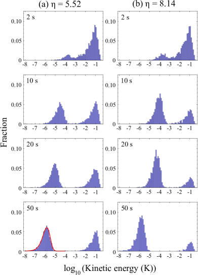
Figure 13: (Color online) Kinetic energy distributions at four different times (2 s, 10 s, 20 s and 50 s) and for two values of the evaporative cooling parameter: (a) $\eta=5.52$, (b) $\eta=8.14$. For comparison, a Maxwell-Boltzmann distribution at 1 $\mu$K is shown by a red line. The coolant is Rb and $a=+1.5\bar{a}$.

Figure 13(a) shows how the kinetic energy distribution of the molecules evolves with time when $\eta=5.52$ and $a=+1.5\bar{a}$. At 2 s, the distribution is similar to the case without evaporation (see Fig. 5(a)), but by 10 s there is a large difference. For this value of $\eta$ the atoms initially cool quickly, many atoms are ejected, and the density gradually increases. About half the molecules cool along with the atoms and these have kinetic energy below 100 $\mu$K at 10 s. The other half remain uncooled because they find themselves outside the rapidly shrinking atom cloud. After 50 s the cold fraction is fully thermalized to the 1 $\mu$K temperature of the atom cloud. Figure 13(b) shows the corresponding evolution when $\eta=8.14$. In this case, the evaporation initially proceeds slowly, and the molecule distribution remains similar to the case without evaporation for the first 10 s. Because the atom cloud shrinks more slowly a larger number of molecules are captured into the cold fraction, and these then cool to 1 $\mu$K on a 50 s timescale.

Figure 14: (Color online) Sympathetic cooling of molecules with evaporative cooling applied to the atoms. Graphs show the time evolution of (a) the fraction of molecules with kinetic energy below 1 mK, when $a=+1.5\bar{a}$; (b) the mean kinetic energy of the ultracold fraction when $a=+1.5\bar{a}$; (c) the mean kinetic energy of the ultracold fraction when $a=-0.5\bar{a}$. (i, black) $\eta=5.52$, (ii, red) $\eta=6.67$, (iii, blue) $\eta=8.14$. In (b) and (c), the dashed lines show how the atomic temperature evolves. The long-dash green line shows the atom temperature without evaporative cooling.

Figure 14(a,b) show the fraction of molecules with kinetic energy below 1 mK, and the mean kinetic energy of that fraction, using $a=+1.5\bar{a}$ and three different values of $\eta$: 5.52, 6.67, and 8.14. When $\eta=8.14$ the atom cloud cools slowly at early times, and this gives the molecules enough time to thermalize with the atoms before the atom cloud shrinks too much. After this initial thermalization to the atom temperature, the molecular temperature follows the evaporative cooling of the atoms very closely. The ultracold fraction is high in this case, reaching 85% after 50 s. However, it takes the full 50 s for this fraction to reach 1 $\mu$K. For this value of $\eta$, the atom density increases by a factor of 70 over 50 s, and the mean atom-molecule collision rate increases from 4 s^-1 to 45 s^-1. When $\eta=6.67$ the atoms cool more rapidly and the cloud size shrinks more rapidly. Consequently, the ultracold fraction of molecules is reduced to 74% but this fraction now reaches 1 $\mu$K in 30 s. When $\eta=5.52$ the atoms initially cool quickly, but the cooling rate slows down as time goes on because the density does not increase rapidly enough to compensate for the decrease in atom velocity. The ultracold fraction of molecules reduces to 59%. The mean kinetic energy of this fraction falls quickly, reaching 100 $\mu$K in 3.4 s, and 10 $\mu$K in 17 s. Therefore, evaporative cooling with a relatively low $\eta$ is a good strategy for cooling rapidly to temperatures above 10 $\mu$K. However, the cooling slows down at longer times and it ultimately takes longer to reach 1 $\mu$K than for the intermediate value of $\eta$.

Finally, we consider the case where $a=-0.5\bar{a}$. This is a highly unfavorable case compared to $a=+1.5\bar{a}$, both because the elastic cross section in the ultracold limit is nine times smaller and because there is a deep Ramsauer-Townsend minimum in the cross section for collision energies slightly below 100 $\mu$K, as can be seen in Fig. 1. We find that the fraction of molecules with kinetic energy below 1 mK is almost unchanged from that shown in Fig. 14(a). This is to be expected since, at energies higher than 1 mK, the cross sections for the two values of $a$ are not too different. Figure 14(c) shows how the mean kinetic energy of the ultracold fraction evolves when $a=-0.5\bar{a}$. Because of the lower collision rate, the mean kinetic energy of the molecules lags behind that of the atoms, instead of the two being locked together as they are in the case of $a=+1.5\bar{a}$. The molecules are slow to reach 20 $\mu$K for all values of $\eta$, because they have to cool through the Ramsauer-Townsend minimum to do so. For $\eta=5.52$, the atoms cool too quickly and the molecules have not thermalized with the atoms even after 50 s. For $\eta=8.14$ the initial cooling rate of the atoms is slow enough that the molecule temperature can more closely follow the atom temperature, both reaching 1 $\mu$K in about 50 s. The cooling of the molecules is fastest for the intermediate value of $\eta$. In particular, the mean kinetic energy of the molecules falls rapidly as soon as it is below 20 $\mu$K, and it reaches 1 $\mu$K in 36 s. We see that, even for this unfavorable value of $a$, evaporative cooling of the atoms can bring the molecule temperature down to 1 $\mu$K on a reasonable timescale, provided a suitable value of $\eta$ is chosen. It is clear that knowledge of the actual atom-molecule scattering length will be needed to choose the optimum conditions for evaporative cooling.

X Conclusions

In this paper, we have addressed the methodology for modeling sympathetic cooling of molecules by ultracold atoms, and we have studied in detail the results of simulations for a prototype case where ground-state CaF molecules in a microwave trap are overlapped with ultracold Li or Rb atoms in a magnetic trap. This work leads to a number of conclusions which we now summarize.

Previous work on sympathetic cooling used a hard-sphere model of collisions based on an elastic cross section. This is appropriate at very low energies (in the s-wave regime), but breaks down badly for heavy molecules in the millikelvin regime. We have shown that a hard-sphere model based on an elastic cross section significantly over-estimates the cooling rate for collision energies above the s-wave scattering regime. A hard-sphere collision model that uses the energy-dependent momentum transport cross section, $\sigma_{\eta}^{(1)}$, gives the correct molecule cooling rate, but underestimates both the heating of the atoms and the loss of atoms from the trap. We have therefore used the full differential cross section to model atom-molecule collisions, so that the cooling of the molecules and the associated heating and loss of atoms are all modelled accurately.

We have studied sympathetic cooling of CaF with both Rb and Li over a range of typical values of the atom-molecule scattering length $a$. We find that Rb offers significant advantages over Li as a coolant for ground-state molecules. The mean scattering length ${\bar{a}}$ is almost twice as large for Rb, and so it is likely that the true scattering length will also be larger for Rb. The mean energy transfer is proportional to $\mu/(m_{{\rm CaF}}+m_{{\rm at}})$ which is 0.48 for Rb, but only 0.19 for Li. If $a$ happens to be negative there can be a deep Ramsauer-Townsend minimum in the cross section. For Li, the minimum typically occurs when $E^{{\rm lab}}_{{\rm CaF}}$ is between 1 and 10 mK, and the molecules cool very slowly because their energies must pass through this minimum. For Rb, the minimum is shifted down an order of magnitude in energy, and so the molecules do not encounter the minimum until they have reached the ultracold regime. For Li, the cooling rate is very sensitive to the actual value of $a$, while for Rb the initial cooling rate is fairly insensitive to $a$ because the Rb+CaF cross section conforms closely to a classical result, independent of $a$, down to temperatures near 1 mK. This brings less uncertainty about the likely results of sympathetic cooling experiments if Rb is used. These advantages of Rb as a coolant are likely to extend to other molecules of a similar or greater mass. Finally, it is experimentally easier to prepare large, dense samples of ultracold Rb than of ultracold Li.

It should be noted that the preference for Rb over Li applies only to ground-state molecules that cannot be lost from the trap through inelastic collisions. For molecules in static magnetic or electric traps, a light collision partner such as Li, Mg or H provides a higher centrifugal barrier than a heavy one such as Rb, and this may be important for suppressing low-energy inelastic collisions Wallis and Hutson (2009); Wallis et al. (2011); González-Martínez and Hutson (2013).

For molecules with an initial temperature of 70 mK, cooled by Rb with a temperature of 100 $\mu$K and a peak density $10^{11}$ cm^-3, we find that, after 10 s, 75% of the molecules have cooled into a distribution with a temperature of 200 $\mu$K. If the initial temperature of the molecules is reduced to 20 mK, this fraction increases to 99% due to improved overlap between molecule and atom clouds. By arranging for the atom trap depth to be far below the initial molecule temperature, we can ensure that the majority of the energy in the molecule cloud is removed by atoms that are lost from the trap, instead of heating the atom cloud. For efficient cooling the atom number should exceed the molecule number by at least a factor of 100. By applying evaporative cooling to the atoms, the molecules can be sympathetically cooled more rapidly, or they can be cooled to far lower temperatures. For values of the scattering length in the likely range, and with a suitable choice of evaporation ramp, 70% of the molecules can be cooled to 1 $\mu$K within about 30 s. These are all encouraging results: using experimentally achievable atom numbers, densities and temperatures, sympathetic cooling to ultracold temperatures can work on a timescale that is short compared to achievable trap lifetimes. A good starting point for such experiments would be a mixed-species magneto-optical trap of molecules and atoms.

Data underlying this article can be accessed at http://dx.doi.org/10.5281/zenodo.32993 and used under the Creative Commons CCZero licence.